Submitted:
29 August 2025
Posted:
01 September 2025
You are already at the latest version
Abstract
The transition to carbon-neutral energy has renewed interest in hydrogen as a gas turbine fuel in the form of fuel blends with hydrocarbons. However, the distinct fluid properties and chemical kinetics of hydrogen and hydrocarbon blends necessitate redeveloped combustor designs. While conventional combustor design and emissions estimation through computational fluid dynamics (CFD) is preferred, it is computationally intensive and impractical for system-level simulations. To alleviate this, a thermofluid network model was developed to predict the performance of a MGT combustor operating on pure and fuel blends of propane and hydrogen. It incorporates sub-component pressure losses and heat transfer, and presents the first implementation of well-stirred and plug-flow reactors into Flownex SE. A 3D CFD study of the combustor revealed that hydrogen addition improved combustion efficiency and reduced wall temperatures. However, despite producing less CO2, it leads to 70 % more CO and 80 % more NO than for propane-only operation. Validated against the 3D CFD data, the network model predicted the combustor's outlet total temperature and pressure within 0.5 % and 0.26 %, respectively. The change in total pressure across subcomponents (< 6%) and the mass flow distribution showed similarly strong agreement. Major species mass fractions, CO2 and H2O, were predicted accurately. However, by assuming that the temperature and composition are uniform within combustion zones, zone and wall temperatures and pollutant predictions deviated considerably. NO was overpredicted by a factor of 8.2–10.7, and CO was overpredicted for propane-only, but underpredicted for blended cases. The network model achieved this performance 420 times faster than CFD, making it suitable for rapid design exploration.
Keywords:
Hydrogen-Propane fuel-blend combustion
; CHT CFD
; Network modeling
; Micro Gas Turbines
; Combustor modeling
; Chemical Kinetics
1. Introduction
Low-emissions combustors, powered by fossil fuels, are a well-developed component of gas turbines. The advent of renewable fuels and a drive towards carbon neutral power generation has revived interest in hydrogen as a fuel [1]. Currently, 98% of the available hydrogen is produced from fossil fuels [2]. To achieve carbon-neutral power production using hydrogen, it must be produced from a carbon free feedstock and renewable energy, commonly termed Green Hydrogen. However, the low availability and high cost of green hydrogen has led to increased interest in hydrogen-hydrocarbon fuel mixtures as a transitional solution, enabling partial decarbonization while maintaining fuel supply security [3]. Hydrogen enrichment in gas turbine combustors is a promising near-term decarbonization strategy. It has been shown to reduce CO and CO2 emissions [4], improve combustor pattern factors [5], enhance flame stability and widen combustor operating limits [3]. These benefits stem from hydrogen’s higher flame speed and improved mixture reaction rate resulting from the increased oxygen (O) and hydrogen (H) radical pool [6, 7]. While hydrogen enrichment offers clear benefits, it also introduces significant challenges which include a higher likelihood of flashback, increased NOx production and higher flame temperatures. These effects may lead to pollution and increased thermal stresses that require careful consideration. Given the disparate fluid properties and chemical kinetics of hydrogen and mixture fuels compared to pure hydrocarbon fuels, may require that combustors be redeveloped to this end.
Typically, the preliminary aerodynamic design of gas turbine combustors begins with the work of Mongia [8], Melor & Fritskyk [9] and Lefebvre & Ballal [10]. This is an empirical approach using correlations derived from experimental data. Despite its simplicity, a design process using empirical correlations can be implemented to reduce a combustor’s pressure losses and pollutant formation and optimise its mass flow distribution in a timely manner. Moreover, these correlations can also be utilized to investigate off-design performance of the combustor. However, due to the data-driven nature of the correlations, working outside of the intended operating conditions may produce unreliable results and may be a limiting factor of this modelling method.
A brief review of literature pertaining to semi-empirical modelling of gas turbine combustors. Despierre, et al. [11] demonstrated the versatility of the network method by optimising an annular combustor with a genetic algorithm. The use of a genetic algorthm was facilitated by the network’s fast solving time and reached an optimum solution. Gouws [12] developed an empirical and network models to reverse engineer and predict the performance and wall temperatures of a can combustor from a T56 Rolls Royce engine. The empirical model estimated discharge coefficients for combustor flow components, but produced mass flow distribution errors of 11.8-35.7% compared to experimental data. Calibrating these coefficients reduced errors but made components non-generalizable. With a calibrated mass flow distribution, average gas and wall temperatures matched 3-D CFD simulations well, with exit temperatures differing by less than 13%. du Toit & Theron [13] developed a conjugate flow and heat transfer network model of the NASA E3 development combustor. Validation of the network model focused on the results for the combustor wall temperatures where an error range relative to 3-D CFD data was calculated to be between 1 % to 13 %. Mahto & Chakravarthy [14] presented a hybrid approach by coupling a network model and a CFD simulation. The mass flow distribtion through the combustor was determined by the network model and the CFD resolved 3-D turbulence and combustion within the flame tube. This combination significantly reduced the mesh size of the CFD simulation and decreased the time to reach convergence. The researchers then performed a complex multi-objective optimisation focussing on the effect of swirl on the blow-off region, and the improvement of combustion efficiency, total pressure drop and pattern factor. Across these studies, researchers utilized emprical pressure loss correlations for diffusers, holes and swirlers to account for the aerodynamic behavior of the combustor. Similarly the heat transfer rates to the liner and casing is performed using empirical correlations for fluid radiation, convection and surface radiation pathways.
Estimating pollutant emissions during combustor design relies heavily on CFD due to the high cost of experimental combustion characterization tests. Furthermore, the computational resources and time required for transient system-wide CFD modeling is also prohibitive. Consequently, gas turbine designers resort to low-fidelity models that represent combustors as networks of zero- and one-dimensional (1D) chemical reactors, known as chemical reactor networks (CRNs) when performing system-wide simulations. With a reduced requirement for computational resources, implementing CRNs enables the use of complex reaction mechanisms and the timeous exploration of a design space [15].
Several studies, Park et al. [16], Fichet et al. [17]; Colorado & McDonell [18]; Kaluri et al. [19], show that CRNs in the study of gas turbine combustors achieve comparable levels of accuracy when compared to CFD in the prediction of combustion completeness and pollutants. In Fichet et al. [17], NO emissions had an error of 3 %. A wide error range of 0-250 % is shown in Kaluri et al. [19] for manually and automatically extracted networks. Park et al. [16] found that the error of the CRN, relative to experimental data, increased at high combustor loading. For all simulated cases in Park et al. [16], the CRN was able to closely replicate the trends for CO though substantial errors were recorded and estimated NO to within 4 ppm. Grimm [20] automatically extracted reactor networks from CFD data and evaluated the effect of network fidelity on accuracy. It was found that networks with at least four reactors were required to reliably predict NO emissions and increasing the network size did not produce substantial improvements. Importantly, it was shown that accounting for reactor heat loss had a more substantial impact on the accuracy of predicted NO concentrations.
Most CRN studies focus solely on chemical reactor configuration and neglect momentum transport within the combustor. Aerodynamic effects (modelled via flow networks) and combustion (modelled via CRN) are typically treated separately. This separation represents a key limitation because combustors are coupled to turbomachines, where changes in mass flow rate and operating pressure can significantly affect combustor performance and pollutant formation. Many of the previous researchers which investigated the aerodynamic performance of gas turbine combustors using the 1-D network modelling approach did include combustion modelling ( Despierre, et al. [11], Gouws [12] and du Toit & Theron [13]). While the techniques implemented by these authors, chemical equilibrium and constrained adiabatic combustion, produced satisfactory outcomes, they are unsuitable for estimating pollutant emissions. Accurate emissions prediction requires complex techniques such as chemical reactor networks (CRNs) or computational fluid dynamics (CFD) modelling. Limited research literature exists that attempts to integrate both 1D aerodynamic networks and combustion kinetics through CRNs into a unified model capable of capturing sufficient detail for system-wide investigation of fuel mixture effects on gas turbine performance. Haytaysal & Yozgatligil [21] attempted to integrate chemical reactors into a flow network. However, the study focused on the solution methods for network models and provided limited results discussion, only including total pressure changes and outlet combustor temperature predictions that correlated well with benchmark CFD results.
Current literature reveals three key gaps: limited investigation of hydrogen-propane mixtures in gas turbine combustors; 1-D thermofluid network studies lacking generalizability due to oversimplified pressure loss treatment; and CRNs rarely integrated with 1-D flow networks to account for aerodynamic changes, limiting model applicability across combustor operating ranges required for system-wide design and off-design performance simulations.
In the present work, the capability of a 1-D thermofluid network model to predict the performance of a can combustor is assessed for fuel mixtures of propane and hydrogen. The network model is constructed in Flownex SE using flow elements to estimate heat transfer and total pressure changes. Well-established pressure loss correlations specific to combustor components are implemented via custom user scripts. For the first time in Flownex SE, Cantera-based well-stirred reactors (WSRs) and plug flow reactors (PFRs) elements are integrated to account for chemical kinetics within the combustion zones. The performance of the integrated thermofluid network model is validated using both CFD simulation results and experimental data for propane only firing, thereafter both the CFD combustor and thermofluid network models are used to estimate combustor performance when firing various degrees of hydrogen mixing with the propane. The novelty of the present work lies in four key contributions: CFD analysis of hydrogen-propane fuel mixture combustion within a gas turbine can combustor, detailed presentation of network modelling methodology and applicable loss models, integration of Cantera-based reactors within Flownex SE, comprehensive validation for propane-only operation, and extension of this validation to both pure and blended fuel mixtures. The present study focuses on developing a standalone combustor network model within Flownex SE, with the objective of future integration into a full-cycle gas turbine model. The resulting unified gas turbine system model will feature a fully generalizable combustor network capable of predicting engine performance and emissions across a wide range of operating conditions.
2. Materials and Methods
2.1. Case Study Gas Turbine
The analysis of combustor performance is conducted for its operation within a twin-shaft Brayton cycle gas turbine with a layout as shown in Figure 1. This is an experimental system currently at the Mechanical and Mechatronic Engineering Department of Stellenbosch University that was developed by Ssebabi [22]. In Figure 1, the alphanumeric labels demarcate the measurement stations and the control valves.
The gas-generator and power turbine configuration is comprised of two Borg Warner turbochargers, the model K31 and K44, as the high and low pressure machines. At a HP turbine rotational speed of 73000 revolutions per minute (rpm) it operates at a compressor total-to-total pressure ratio of 2.1 and combustor outlet total temperature is 840 °C. With the LP compressor as the load, at the above operating conditions, the machine was estimated to produce 6.5 kW at a thermal efficiency of 3 % [22].The system is designed for propane-only operation, and work is currently underway to evaluate its performance experimentally with hydrogen and propane fuel mixtures. This study forms part of that investigation. The combustor boundary conditions used to evaluate the network model are based on experimental data from Ssebabi [22], presented in Table 1.
2.2. Modelling Theory
2.2.1. Thermofluid Network Modelling
In a system modelled by the finite volume method (FVM) thermofluid network approach, components are represented as 1-D flow elements connected to 0-D nodes to form a network, an example of which is shown below in Figure 2 (left). This discretisation is analogous to the traditional 3-D CFD approach where, the domain is discretised into cells with faces and cell centroids (Figure 2 [right]). In the thermofluid network approach, the mass and energy balance equations are solved at nodes, and the momentum balance equations are solved at flow elements, creating a semi-staggered grid type numerical approach [24]. Closure of the mass, energy and momentum balances are through semi-empirical or empirical component characteristic models for friction (e.g. Darcy-Weisbach correlations), heat transfer (e.g. Dittus-Boelter internal convection correlations) and work (e.g. Euler turbomachine equation). All thermofluid properties such as pressure and temperature are stored at nodes while source terms such as heat transfer rates and pressure losses are stored at elements, along with mass flow rates.
Shown below in equations (1) to (3) are the differential forms for the steady-state 1-D conservation equations for mass, energy, and momentum, respectively.
In the above equations, [kg/s] is the fluid density, and [m] is the spatial dimension. On the left-hand-side (LHS) of the energy equation, [m/s] is the fluid velocity , [J/kg] is static enthalpy, [m2/s] and [m] are the gravitational acceleration constant and the elevation of the system respectively. On the right-hand-side (RHS), the volumetric heat transfer rate to the fluid and the volumetric work done by the fluid interacting with its surroundings is represented by [W/m3] and [W/m3]. Finally, on the RHS of the momentum balance, [Pa] is the fluid static pressure, [Pa] is the total pressure rise due to work interactions, and [Pa] is the total pressure loss across the fluid element due to friction or secondary losses.
Through the volume integration of the differential equations and applying the above-mentioned discretization approaches, the steady-state mass and energy balance equations for fictitious node i are equations (4) and (5). In these equations, [kg/s] represents the mass flows rates from nodes i to the successor (downstream) nodes s, along that edge between these nodes. Similarly, represents the mass flow rates along the edges between the predecessor nodes p and the node i. In the discretized integral-form energy balance equation, [J/kg] is the stagnation enthalpy of node i and [J/kg] is the stagnation enthalpy of the predecessor nodes p connected via edge . [W] is the heat transfer rates calculated along edge and similarly [W] is the work transfer rate along edges .
To correctly account for the compressible nature of the flow in the combustor, the differential momentum equation should be treated accordingly. As a first step, the derivative on the LHS of equation (3) is expanded using the product rule as shown in equation (6). The second term on the LHS of the below equation is zero for steady-state flow due to the divergence-free condition from the mass conservation equation.
The momentum equation for compressible flow is written in terms of total pressure ( [Pa] and temperature () [K]. To do so, the theorem in equation (7) is substituted into equation (6) [25].
The result is the momentum equation for compressible flow shown in equation (8).
Finally, the discretised differential equation for compressible momentum is written as shown in the equation below, where and subscripts indicate the downstream and upstream nodes respectively. is the stagnation nodal pressure, the nodal stagnation temperature, work input along edge and pressure loss along edge . The remaining overbar properties are the average properties calculated at edge , using a linear averaged approach and the properties at the upstream and downstream nodes.
Equations 4, 5 and 9 are the generalised form of the discretised difference equations that are solved in a network modelling approach to determine changes in a system’s pressure, enthalpy, and mass flow rate. These are coupled with the necessary fluid properties and characteristic models for friction, heat transfer and work which will be discussed in the next sections.
2.2.2. Combustor Aerodynamic Loss Models
A can RQL combustor is shown in Figure 3. It is comprised of multiple aerodynamic features, highlighted in the upper portion of the diagram. These are the inlet pre-diffuser (1), snout (2), annular passage (3), axial swirler (4), annular passage (5), primary holes (6), secondary holes (7), flame tube (8) and the outlet diffuser (9).
In the current work, unless stated otherwise, we will use the loss models of Lefebvre [26] and Lefebvre & Ballal [10] to determine the pressure losses through the pre-diffuser, snout, swirler and dilution jets, and the recirculation mass flow rates due to swirl and dilution jets. The changes in pressure for the rest of the combustor can be modelled by existing components within Flownex SE. The total pressure loss through a prediffuser is calculated through equation (10) [27].
A similar equation is used, shown below in equation (11), for the pressure loss through the snout:
For a straight bladed axial flow swirler the total pressure drop is calculated using the following equation.
In the previous equation, is a constant that differs based on the vane shape (flat or curved) and is the vane angle. For a flat vane, which is the type used in this study, it is 1.3 and 1.15 for curved. The total pressure drop is dependent on the liner cross sectional area, [m2], and the swirler annulus area, [m2]. The swirling flow will cause flow reversal i.e. flow recirculation known as the entrainment mass flow [kg/s]. As shown in equation 13, from Lefebvre [26], the average entrainment mass flow in the primary zone is dependent on the swirl number ( in equation 14) which is a geometric indicator of the swirl intensity and the length of the primary zone, [m].
For the current combustor, the recirculation of mass flow rate into the primary and secondary zone may also be induced through opposing jet flow as shown in Figure 4.
The mass flow recirculated by opposing jets, [kg/s], is a function of the jet’s angle of entry into the combustion zone, and the temperature ratio between the jet inlet and the respective combustion zone. To estimate the angle of entry, firstly, the jet’s loss coefficient is calculated as in equation 15.
Here, is the ratio of the jet’s dynamic pressure to the dynamic pressure in the annular passage just upstream of the jet. Similarly, is a ratio of a single jet’s mass flow rate to the mass flow of the annular passage upstream of the jet. The asymptotic discharge coefficient, , is determined in equation (15) as approaches infinity. Finally, the rate of recirculated mass flow is calculated as shown in equation (16).
is the mass flow rate of a single jet and is the jet’s angle of entry into the combustor’s flame tube. is the temperature ratio between the jet inlet () [K] and the respective combustion zone () [K].
2.2.3. Chemical Reactor Network Models
Chemical reactor models couple the equations describing the chemical, thermodynamic and fluid dynamic processes within a chemically reacting system [28]. There are numerous formulations for chemical reactors, each with assumptions that characterise specific operating conditions. Reactor zones within a conventional combustor, can be considered as constant volume and pressure processes that may be modelled by a WSR and PFR [29, 10, 28]. The conditions assumed within the reactors are that oxidant and fuel are fed constantly and mix rapidly. Under these conditions, the reactions occur uniformly resulting in a uniform reactor temperature and composition. The following discussion will present the equations used in Cantera [30] for the simulation of combustion in a WSR and PFR.
Equation (17) presents the unsteady form of the mass conservation equation written for a single chemical species, , in a WSR. It states that the change in mass of a species depends on the mass generation or consumption of the species by chemical reaction through the term , where [mol/m3s] is the net reaction rate per unit volume, [m3] is the reactor volume and [kg/mol] is the molecular mass of the species. The formulation also considers multiple inlet () and outlet () mass flow streams, where is the mass fraction of species at the inlet and is the mass fraction of said species leaving the reactor.
The energy conservation equation (18) is written in terms of temperature where [W] is the net rate of heat addition to the reactor from external sources. Term [W], describes the combustion heat release of the mixture as a sum of products of specific enthalpy ( and the rate of mass consumption/ generation () of the species resulting from the chemical reactions.
In a PFR, reactants and products flow axially under ideal frictionless conditions. The gas mixture is an ideal gas, and the composition is considered uniform perpendicular to the flow, reducing the problem to a one-dimensional analysis. Although the PFR is a steady-state system, it captures the effect of residence time on chemical kinetics by integrating the species’ net production rates over the flow-through time through the reactor. The governing differential equation for the evolution of a species mass fraction through a 1-D domain, in a PFR, is given in the equation below.
In the above equation, the change in species mass fraction, , is determined along the flow path in direction [m] at a velocity [m/s]. Similarly, the energy equation (20) is formulated to estimate the change in temperature () [K] where and is the mixture specific heat and density, respectively. The term , is the heat released due to combustion. is the species molar enthalpy and the net reaction rate per unit volume as discussed earlier.
A generalised and compact form of the net reaction rate is shown below in equation (21). This form accounts for elementary reactions and species that contribute to the reaction rate of a single species (). This form is required when implementing large reaction mechanisms like the GRI-Mech.3.0 [31] for hydrocarbons.
and are matrices of the stoichiometric coefficients for the reactants and products, respectively. The term is the product of terms of the molar concentration of each species in the reaction mechanism raised to its stoichiometric coefficient .
In equation (21), the rate coefficient is in the modified Arrhenius form, equation (22), where the subscripts and is for the forward and reverse reaction, respectively.
The magnitude of the rate coefficient is determined by the pre-exponential factor (), static temperature of the reactants () and the activation energy (). The temperature exponent (), pre-exponential factor and activation energy are empirical constants specific to the reaction mechanism, and is the universal gas constant.
2.2.4. Heat Transfer Modelling
In this study, heat transfer is considered within the flame-tube, annular passage of the casing, and to the environment only.
Convective heat transfer between the fluid and solid in the combustor is modeled using the Dittus and Boelter heat transfer coefficient calculated in equation (23). Here, [W/m²K] is the fluid conductivity, [m] is the hydraulic diameter, is the Reynolds number and is the Prandtl number. The constant is 0.4 if the fluid is being heated and 0.3 if the fluid is being cooled. Despite being formulated for inner tube heat transfer, equation (23) can be applied to an annular passage by using the annulus’ hydraulic diameter (Dout - Din) [32].
Fourier’s Law determines the rate of heat transfer through solid objects while equation (24) is used to model the radiation heat transfer rate. is the surface emissivity, [W/(m²·K⁴)] is the Stefan-Boltzmann constant, T [K] is the temperature of radiating () and receiving () surfaces.
The emissivity of luminous flames () from Lefebvre and Ballal [10] is utilized to estimate gas-to-solid radiation as shown in equation (25). This expression considers the effects of fluid pressure (), and air () and fuel () mass flow rates on radiation. It accounts for effect of water vapour on luminosity () by including the fuel hydrogen mass fraction (. The mean beam length in the combustion zone is calculated as where [m3] is the reactor volume and the [m2] is the area of the reactor. [K] is the temperature of the fluid () and the wall ()
Fluid absorptivity () is related to the emissivity through the temperature ratio between the fluid and the wall, as shown in Equation (26).
2.2.5. CFD Modelling
To simulate steady-state turbulent flow in a combustor, the Reynolds Averaged Navier-Stokes (RANS) equations are utilised. In numerical studies of similar combustors, RANS simulations using the Realizable k-ε turbulence closure is often employed to predict hydrogen and mixed fuel combustion accurately when compared to experimental results [33, 34, 35]. The Realizable k-ε formulation is more computationally economical than the k-ω Shear Stress Transport (SST) model and comparably capable of modelling flows with adverse pressure gradients, separation and reverse flow caused by swirl as seen in a combustor [36, 37]. Therefore, in the present work, turbulence closure is accomplished using the Realizable k-ε turbulence model with non-equilibrium wall treatment.
The RANS continuity, momentum and energy balance equations solved by Ansys Fluent version 24R2 are shown in equations (27), (28) and (30) respectively.
In the above equations, is the mean density of the fluid which is, for an ideal gas mixture, based on the mass fraction weighted sum of the species molecular weight. and are the velocity and spatial dimension in direction , respectively. In the momentum equation (28), is the static pressure, is the turbulence kinetic energy and is the Reynolds stress term which, through the Boussinesq hypothesis, is modelled using equation (29). The turbulent viscosity, , introduced by equation (29) is calculated as where is the turbulence dissipation rate. In the Realizable formulation, is a function of the mean strain and rotation rates, the angular velocity of the system rotation, and and [38].
When using the partially premixed combustion model in Ansys Fluent (discussed later), the total enthalpy () formulation of the energy equation is implemented as shown in equation (30) [38]. Total enthalpy includes the species enthalpy of formation and therefore accounts for the heat released during combustion. As such, the heat released due to combustion is not included in the source term, , of equation (30).
Turbulent viscosity is used to determine the effective thermal conductivity () of the fluid seen in equation (30), . Here, is the fluid thermal conductivity and the turbulent Prandtl number, , is a constant value of 0.85.
The heat transfer interaction between fluid and solid material is considered in this study. A Conjugate Heat Transfer approach is implemented where the fluid and solid media form a single and continuous mesh. Equation (31) is the energy balance equation for the solid media only. It accounts for convective heat transfer as a result of moving walls (first term on RHS), conduction (first term on LHS) and a volumetric heat source term. is the velocity vector of the wall, is the sensible enthalpy, is the conductivity of the solid and is the volumetric heat source term.
Convective heat transfer between the solid and fluid domain is modelled using the law-of-the-wall for non-dimensional temperature as seen in equation (32) [38]. Here, on the LHS, is the wall temperature, is the temperature of the wall adjacent cell-centroid, is calculated as . The first term on the RHS ) determines the convective-conductive heat transfer through equation (33). The equations available to calculate are implemented based on the height of the viscous () and the thermal sublayer () where is an empirical and is the von Kármán constant. is a function that accounts for the influence of roughness and the Prandtl number on heat transfer in the laminar sublayer.
The second and third term on the RHS of equation (32) are included to account for compressibility effects when using pressure-based solvers. and are the turbulent kinetic energy and mean velocity at the wall adjacent cell-centroid.
Radiation is modelled using the discrete ordinance (DO) model, with four angular divisions and three pixels in both the azimuthal (phi) and polar (theta) directions. The fluid absorptivity is determined through the weighted-sum-of-grey-gasses method (WSGGM), only considering the tri-atomic molecules of CO2 and H2O. Radiation scattering is negligible and, therefore, neglected since the radiating medium is gaseous.
The evolution of the reactant and product species through the domain is modelled in the present work using the partially-premixed combustion approach. Turbulence-chemistry interaction is modelled using the non-adiabatic FGM model coupled with the full GRI-Mech 3.0 reaction mechanism [31] for hydrocarbons. The Zimont turbulent flame speed model is implemented for premixed combustion, and the progress variable variance is treated as a transported scalar. To account for mixing and chemical timescales, the turbulent flame speed setting is selected for turbulence-chemistry interactions. Laminar flame speed is estimated using the Metgalchi-Keck law [39] for propane, and the precomputed PDF values are used for hydrogen and fuel mixtures. In ANSYS Fluent only the mass fractions of CO and CO2 are considered for hydrocarbon combustion with a weight of unity, ensuring that the progress variable increases through the flame [38]. Since CO exists in small quantities relative to CO2 within a combustor, the mass fraction of CO2 will bias the progress variable towards 1. This may cause non-physical behaviour since the FGM model will regard a mixture as burnt when the progress variable is close to or equal to 1 (high CO2 concentrations), causing reaction progress to slow or stop. Therefore, in the standard FGM model, when combustion is only mapped using the progress variable, the estimation of slower evolving species like NO and the post flame burnout of CO is inaccurate [40, 41]. To remedy this, as suggested by Klarmann, et al. [40] and Efimov, et al. [41], transport equations for CO and NO mass fractions are solved and their net reaction rates are corrected based on the transported values.
2.3. Model Development
In the following section the above thermofluid network theories (flow equations, pressure losses, CRNs and heat transfer) will be applied to model the case-study gas turbine combustor. Furthermore, the 3-D CFD model setup of the combustor will also be discussed. Firstly, the three experimental running points simulated will be discussed along with the various propane-hydrogen mixture simulation boundary conditions.
2.3.1. Simulation Cases
Initial validation of the CFD and network models will be performed for propane-only operation. To this end, the experimental results of [22] are used as simulation boundary conditions. 3 engine running points have been chosen across the systems operating curve resulting in 3 simulation cases. Running point MGT3 is considered the primary operating point as it is closest to the design point of the system.
Once the CFD and thermofluid network models are validated using the propane-only experimental data, the effect of hydrogen blending is investigated. Since there is no experimental data available for the hydrogen-blending operating points, the CFD simulations will be used as the ground truth when investigating the network model accuracy. For the three cases (MGT1-MGT3), different hydrogen blending ratios are simulated. The pure hydrogen mass flow rates were selected to achieve outlet combustor temperatures similar to that of pure propane combustion for the three running points. Table 2 below shows the mass flow rates for pure propane and pure hydrogen operation.
The blending ratios were defined based on the nominal fuel mass flow rates for the pure fuel conditions. For example, for the 75-25 ratio (propane-hydrogen), the fuel flow rate for MGT3 is 75% of the nominal mass rate flow of propane (0.0045 kg/s) and 25% of the nominal hydrogen mass flow rate (0.0018 kg/s). For input simplicity in CFD, the total fuel mass flow rate is 0.0033 kg/s with a 0.883 mass fraction of propane and 0.117 mass fraction hydrogen.
Table 3 summarizes the mass flow rates and corresponding species mass fractions for all mixture operating points. This method of blending fuels ensures matched outlet temperatures across cases. Doing so will allow a direct comparison of the CFD data for all fuel compositions to determine the effect of hydrogen addition on combustor performance.
2.3.2. 3-D CFD Model Setup
The domain used in the 3-D CFD simulation is shown in Figure 5. As illustrated, the inlet boundary conditions are the air and fuel mass flow rates and the static temperatures of each stream. The compositions of the fuel and air are specified in the setup of the FGM model as mass fractions of the species in the fuel and oxidiser streams. Therefore, for each boundary condition, a mixture fraction is specified which is 1 for the fuel and 0 for the air (oxidiser). A static pressure outlet boundary condition is specified at the outlet of the combustor.
Figure 5 (bottom) shows an isometric view of the combustor highlighting the segmented volumes corresponding to the combustion zones and outlet transition duct (nozzle). These zones are present in the generated mesh and thus available in Ansys Fluent for post-processing purposes. The segmentation enables the extraction of mass-weighted average quantities from each zone for direct comparison with the network model.
The FGM model is implemented using the nonadiabatic diffusion flamelet formulation with full GRI-Mech 3.0 reaction mechanism and the accompanying thermodynamic and transport properties. The fuel and oxidiser were specified as mass fractions corresponding to each running point and fuel mixture in Table 2 and Table 3 with the respective inlet temperatures. The outlet static pressure of the combustor is operating pressure for the generation of the flamelet and PDF table. This pressure corresponds to the operating value specified in the operating conditions of the simulation and therefore the combustor outlet gauge pressure is 0 Pa for all cases.
As suggested in ANSYS [38], for large chemical mechanisms, the absolute error tolerance in the Flamelet generation process was reduced to 1e-20 and the relative error tolerance to 1e-05. The Automated Grid refinement of the Flamelet table was implemented with a maximum change in value ratio of 0.35. The initial scalar dissipation value was reduced to 0.001. The maximum number of flamelets was increased to 400, and the number of grid points in the table was increased to 64 in the mixture and reaction space which improved simulation stability. In the PDF table parameters, the minimum temperature of 260 K was set well below the lowest temperature provided in the boundary conditions, and the number of species in the PDF table is 20.
To model heat transfer, the solid components of the combustor seen in the isometric view of Figure 5 were included in the mesh for a CHT simulation. The solid-fluid wall interfaces of the mesh are therefore coupled to the energy solution, and the exterior wall of the casing is allowed to radiate to the surroundings. Radiation within the combustor is modeled using the DO method with four angular divisions and three pixels in both the azimuthal (phi) and polar (theta) directions. The absorption coefficient is determined using the WSSG method where the beam length is based on the domain.
Pressure and velocity are coupled, with spatial gradients calculated using the cell-based least squares method. Pressure is discretized using the PRESTO! approach, and all equations are discretized using a second-order upwind formulation, except radiation, which uses first-order upwind. The pseudo-time method is implemented with a global time step to enhance simulation stability.
2.3.3. Mesh Independence Study
The 3-D domain was discretised into a poly-hexcore mesh. Care was taken to ensure that the y-plus values were between 30 and 300 for the non-equilibrium wall treatment. Two mesh refinements were performed and evaluated for a grid-independent solution. In Figure 6, the static temperature and velocity magnitude along the axis of the combustor for the coarse, medium and fine mesh are plotted for MGT3. The results show that minor differences in temperature and velocity predictions are observed moving from the medium to fine mesh.
To further demonstrate that the medium mesh is appropriate and mesh independent, the GCI values for outlet total temperature and inlet total pressure were estimated. The results are shown in Table 4 below.
For both temperature and pressure, low GCI values are estimated with a range of 0.00% to 0.12% indicating a high degree of numerical precision for the medium and fine mesh. The refinement ratio is 1.3 or greater, indicating satisfactory refinement [42]. In addition, despite having significantly less cells, the results of the medium mesh deviate only slightly from the fine mesh. Consequently, the medium mesh was selected for further use in this study due to the lower computational cost and levels of precision and accuracy comparable to the fine mesh.
2.3.4. Thermofluid Network Model Setup
The 1-D network model, shown in Figure 7, has been constructed in Flownex SE. The model was developed with an emphasis on simplicity, while being informed by 3-D CFD results. As such, the network model closely represents the layout introduced by Bragg [43], where the primary combustion zone is assumed to be a WSR and post-flame burnout is modelled using PFRs.
Standard flow elements are used to model heat transfer and all flow passages. Jets (holes) are modelled as restrictors with discharge coefficients; other sub-components are modelled using pipe elements with loss coefficients for frictional and obstruction losses. The recirculation effects within the combustor, discussed later, are approximated by redirecting mass flow through flow resistance elements with prescribed mass flow rates. Discharge and loss coefficients, as well as recirculation mass flow rates, are determined by the correlations in Section 2.2.2. The calculations are performed by embedded MathCad user-defined scripts, which are executed after each iteration and update the corresponding flow element parameters until convergence is achieved.
Flownex SE can execute Python scripts within its C# scripting components through PythonNET. This facilitates the use of Cantera WSR and PFR in Flownex SE. In this network model, a C# script is executed within a compound component. It obtains the reactor mass flow rate, inlet temperature, pressure, and list of reactant mass fractions and sends it to the Python script that executes the Cantera reactor calculations. An exit temperature and a list of product mass fractions is then returned to Flownex SE and written to the outlet of the pipe element used to approximate the combustion zone in the flow network.
The results of the 3-D simulation were used to inform the shape of the network. Shown in Figure 8 are streamline traces initiated from the PZ jets (left) and the SZ jets (right). It is evident that there is recirculation into the PZ from the flow entering through the PZ jets. This flow phenomenon is not present in the SZ. The magnitude of the reculation mass flow is estimated using equation 15 from Lefebvre [26] instead of being informed by the CFD. This is, of course, a crude estimation as the correlation does not account for swirl flow within the flame tube and the recirculation zone upstream of the opposed PZ jets. Furthermore, consistent with the mechanism described in Lefebvre [26], recirculation flow induced by swirl, is approximated in the network model. This is achieved by returning products at the outlet of the PZ to its inlet at a rate determined by equation 15. Mass flow entrainment due to swirl is critial for flame holding in this combustor as entrained hot reaction products mix with incoming unburnt reactants in the primary zone to sustain combustion.
The type of reactor used to model each reaction zone was informed by the average Damköhler number of each combustion zone in the CFD results. The Damköhler number was calculated as a ratio of the combustion zones average Kolmogorov time scale to the rate coefficient of the slowest reaction estimated at the average combustion zone temperature [44]. In Figure 9 are three plots for each running point. The plots mark the Damköhler number of each combustion zone for three trends that represent three fuel compositions, namely: propane-only (100-0), hydrogen-only (0-100) and a 50 % share of each fuel (50-50).
Notably, the Damköhler number is much less than 1 for all zones in each data set. This indicates that each zone is mixed sufficiently such that the reaction rates will be chemically limited. Therefore, for the combustor in this study, the selection of WSRs to approximate the PZ and SZ is justified. The DZ also exhibits chemically limited combustion, and it is modelled as a PFR to account for the effect of an increased residence time and elevated reaction temperature on reaction kinetics.
3. Results and Discussion
This section presents the results of the 3-D numerical and network model. First, 3-D CFD results for combustor operation using propane, hydrogen and propane-hydrogen fuel mixtures are presented. The intent is to develop an understanding for how hydrogen supplementation may augment combustor operation. Secondly, a detailed validation of the network model is carried out for propane only operation. Finally, the network model is validated for operation on fuel mixtures of hydrogen and propane.
3.1. 3-D Numerical Model
The experimental data available to validate the CFD model is limited to the combustor outlet total temperature at various running points as recorded in Ssebabi (2020) for propane-only operation (see Table 1). Although the validation dataset is limited, an agreement with the outlet total temperature is considered sufficient for this study as the CFD results will be used to validate a system-level thermofluid network model. A detailed validation of the internal flow structure and flame dynamics is beyond the scope of this work since the network model’s predictive accuracy at the outlet of the combustor is of primary importance.
The CFD and experimental results for the combustor outlet total temperature are presented in Table 5. The CFD model is shown to predict a combustor outlet total temperature 64 K to 85 K lower than the experimental results of Ssebabi [22]. This represents a 5.9 % (MGT1) to 7.6 % (MGT2) difference which is within the typical error range of approximately 5 % and 7 % found in the CFD validation studies of combustors in Cam, et al. [45] and Benaissa, et al. [46], respectively. The close agreement in the outlet total temperature suggests that the combustion and heat transfer processes are captured reasonably well by the numerical model for its intended application.
Figure 10 is a compound figure that displays the change in key combustor parameters with the increase in hydrogen fuel content for each running point. Figure 10-1a is the PZ equivalence ratio and 1b is the global equivalence ratio. Figure 10-2a and 2b are plots for the change in total inlet air and fuel pressure pressure, respectively, normalised to the data for propane only. Figure 10-2c shows the combustor efficiency as a function of blending ratio.
Seeing as hydrogen has a higher mass energy density compared to propane, it is observed that the equivivalence ratios reduces as the blending ratio is increased. Despite common operating conditions for each fuel mixture, the change in total pressure across the combustor varies with changes in fuel blending ratios as seen in Figure 10-2a. The trends for MGT2 and MGT3 are similar, initially decreasing, then increasing from blending ratio 50-50 to pure hydrogen operation. When compared to propane only, the change in total pressure across the combustor is at most 3.5 % and 2.1 % higher for MGT2 and MGT3, respectively. The change in total pressure for MGT1 is lower for all blending ratios. Expectedly, and due to hydrogens lower density, increasing its share in the fuel mixture increases the fuels total inlet pressure (Figure 10-2b). Noteably, the maximum inlet total fuel pressure is for the 25-75 mixture for all running points, and not for hydrogen only operation.
Data for combustion efficiency presented in Figure 10-2c is estimated by comparing the total outlet enthalpy of the CFD simulations to the values estimated by a well-stirred reactor for the same boundary conditions. Operating point MGT3 is closest to the design point and has the highest combustion effiency of 89 % for propane-only operation. It is followed by MGT2 and MGT1 with values of 79 % and 66 %, respectively.
For the fuel blends, when compared to propane-only operation, there is an increase in efficiency for all operating points. In the data for the first blending ratio 75-25, when compared to pure propane, MGT1 displayed the largest increase of 22 % followed by MGT2 with 14 %, and 4 % for MGT3. In addition, there is a narrow combustion efficiency range for the fuel blends where MGT2 and MGT3 have a similar range of between 89 % and 93 %, and MGT1 is between 88 % and 90 %. For pure hydrogen operation, the combustion effiency of MGT1 and MGT2 is increased to 89 % from 66 % and 79 % and the efficiency of MGT3 is unchanged from propane-only operation at 89 %.
It is clear from the above observation that fuel blending with hydrogen improves combustion efficiency, especially at off-design operating points. This is attributed to the enhanced chemical kinetics of the H2-O2 reaction mechanisms. However, for the current combustor, the combustion effiency is not improved when operating close to the design point on pure-hydrogen.
Figure 11 is a compound figure. It presents mass average data (static temperature and species mass flow rate) calculated at the inlet and outlet planes of each combustion zone. The planes at the interfaces of zones are labelled with the abbreviations of both zones. All plots are concerned with running point MGT3 only.
Similar to the work of Tamang & Park (2023) , the CFD data shows that increasing the share of hydrogen reduces the mass fraction of CO2 (Figure 11-c) and increases NO (Figure 11-b) at the outlet of the combustor. CO2 decreases with increasing hydrogen content due to the reduced carbon mass in the fuel mixture, as hydrogen blending is optimized to maintain outlet gas temperatures equivalent to pure propane combustion.
There is no fuel bound nitrogen available to form NO, and the formation of Prompt-NO is suppressed due limited availability of CxHy radicals in the current combustor under the fuel-lean conditions. Therefore, the Thermal-Zeldovich route is the dominant NO formation pathway as tempertures in the PZ and SZ exceed 1500 °C [47]. This verifies the increased net formation of NO with increasing hydrogen as the effective flame temperature is simultaneously increased due to reduced flame radation [48]. In Figure 11-b for the mass flow rate of NO, the hydrogen only case is shown to produce 1.8 times more NO than the propane only case at the outlet of the combustor, similar margins to those reported in Benaissa, et al. [46]and Tamang & Park [5]. Hydrogen addition causes the mass of NO to peak in the SZ before sharply declining in the DZ which is a shift upstream relative to the results for pure-propane operation. It occurs because hydrogen's enhanced combustion kinetics, driven by increased OH, H, and O radical concentrations, accelerate NO formation through thermal, NNH, and N2O pathways compared to propane combustion [49].
For propane only operation, NO formation in the PZ and SZ occurs at a lower rate when compared to fuel blend and pure hydrogen operation (Figure 11-b) despite similar zone temperatures (Figure 11-a). A fuel rich PZ and SZ, for pure propane firing, increases the presence of CxHy radicals necessary for NO reburn, and a high temperature would promote Thermal NO formation [47]. These are competing mechanism and would explain the reduced NO formation rate. As CxHy radicals are consumed in the SZ and DZ of the combustor, the NO reburn rate will decrease increasing the dominance of the thermal pathway. However since dilution air entering the DZ, after plane SZ-DZ, lowers fluid temperatures below the threshold for Thermal NO formation, other NO formation pathways like the Prompt, N2O and NNH will be prominent.
Less CO2 is formed for blended fuels (Figure 11-c), however, an increased share of hydrogen in the fuel is found to reduce conversion rates of CO to CO2. This is evident in Figure 11-d, where the outlet CO mass flow rate for mixture fuels is found to be 1.38 (25-75) to 1.7 (50-50) times more than the propane-only case. Despite being an indication of incomplete combustion, the large variation and concentration of fuel intermediates (not shown here) is found to be beneficial for CO conversion in propane-only combustion. At the low temperatures in DZ, these hydrocarbons increase CO conversion to CO2 primarily through indirect pathways with O and H radicals [28]. With a much larger O an H radical pool in fuel mixture combustion, an increased rate of hydrogen abstraction subverts this effect by forming fewer and lighter hydrocarbons which limit the available CO to CO2 reaction pathways.
Figure 12 shows the area-averaged wall temperatures for the simulated cases and blending ratios per case. Wall temperatures for propane operation show a monotonic upward trend, with PZ and SZ walls averaging 734-754 K and DZ walls ranging 1031-1038 K across all operating points. Both hydrogen mixtures and pure hydrogen reduce zonal wall temperatures compared to propane. The most significant reduction occurs in the PZ of the 50-50 mixture for MGT1 (normalized temperature of 0.71), while the smallest reduction is in the SZ of the 75-25 and 25-75 mixtures for MGT3 (0.884).
The DZ wall is highlighted by the rectangles in Figure 13. Static temperature contours reveal that propane-only operation exhibits active combustion along the DZ wall due to fuel accumulation in this region. Hydrogen introduction increases fuel velocity through the flame tube centre, preventing wall-bound fuel accumulation and combustion. This change, combined with reduced flame radiation from increased water vapor content in hydrogen combustion products, successfully lowers PZ and SZ wall temperatures under blended firing configurations [48, 50].
3.2. Thermofluid Network Model Validation Using CFD Results for Propane-Only Firing
In this section the network model is validated by benchmarking it against CFD results for propane-only operation using the running points found in Table 1. Validation is achieved through a comparison of the mass flowrate distribution, outlet total temperature, change in absolute total pressure and the mass fractions of major and minor species at the combustor outlet. Subsequently, the network model’s ability to predict combustor performance on mixed fuels is determined by comparison with the CFD data presented in the previous section.
The CFD results for outlet total temperature (OTT) and absolute pressure (OTP) is shown in the left-hand plot of Figure 14 for each running point. The error of the network model’s estimates for OTP and OTT, relative to the CFD, is shown in the right-hand plot. The network model predicts higher outlet temperatures than CFD but maintains consistent trends, showing temperature increases from MGT1 to MGT3 with less than 0.5% relative error. Outlet temperatures differ by an average of 5.69 K ± 0.29 K across all operating points. Inlet pressure predictions show excellent agreement with CFD, with relative errors ranging from 0.14% (MGT1) to 0.26% (MGT3).
Figure 15 presents the mass flow rates for each combustor flow path from both CFD and network model simulations, along with the corresponding total pressure drops per flow path. The total pressure drop across each component and the resulting mass flow rate is determined by the loss models presented in Section 2.2.1. The network model underestimates total combustor pressure drop by 3-4% compared to CFD. While cooling holes and pre-diffuser show the largest deviations (6% and 8% respectively), they contribute only 6.3% of total pressure drop. The major pressure drop components (snout, SZ jets, and PZ jets) show better agreement with maximum deviations of 3%, 3%, and 6% respectively. Despite the difference in the change in total pressure across each sub-component, the mass flow distribution predicted by the network model closely agrees with the CFD results.
Averaged inner wall temperatures (left) and zone temperatures (right) for each combustion zone, as estimated by the CFD, are shown in the top row of compound Figure 16. The bottom row shows the errors of the network model relative to the CFD.
The average combustion zone temperature estimated by the network model displays a similar trend to the CFD. Zone temperatures increase from the primary to the secondary zone and subsequently decreases in the dilution zone. This behaviour is expected as the primary zone jets supply air to complete combustion in the secondary zone increasing the average zone temperature, and the dilution zone jets (DZ) then quench the gas entering the dilution zone. Despite similar trends to the CFD data, the network model estimates lower average zone temperatures for all running points. The network model underpredicts the PZ temperature with a percentage error range of -9.6 % to -18.3 %, and a temperature difference of between -109 K to – 238 K. The SZ has an error range between -11.8 % (-197.5 K) and 1.2 % (19.2 K). The DZ is well predicted with an error of -3.4 % or -36.4 K
There is good agreement between the CFD and network model for the inner wall temperatures of the PZ and SZ for MGT1 and MGT2, with errors between -2.5 % and 7.3 %. For MGT3, the SZ wall temperature correlates well with an error 6.4 %, however the PZ wall temperature is under predicted by 15.5 %. Large errors are observed for the DZ wall temperature of all running points with an error range between –16.2 % and – 21.13 %.
The current network model is configured to estimate the convection heat transfer between a combustion zone, represented as a single flow element, and the solid node of the conduction heat transfer element. As such the difference between the average combustion zone temperature and the temperature of the solid node is used to estimate convection heat transfer. In contrast, considering a FVM CFD simulation, convective heat transfer is determined between the wall and the neighboring cell(s) only. Therefore, CFD simulations can account for localized changes in the flow field and combustion, and their effects on gas temperatures and heat transfer. This explains why, despite the low errors in the estimates for the DZ temperatures, there is a large error in the wall temperature estimates.
The network model has demonstrated satisfactory agreement with the CFD model in predicting the global operating conditions, internal aerodynamics, and heat transfer within a can combustor. The distinguishing feature of the network model in this study is the coupling of the aerodynamics with the chemical reactors. The following section of the validation is performed to show that by including chemical reactor models, the network model can predict changes in major and minor combustion species, and the pollutant NO across a system operating curve. Doing so positions the network model as a tool to improve combustion efficiency and pollutant emissions.
The top row of Figure 17 shows plots of CFD data only for the major species mass fraction (left), and the minor and pollutant species mass fraction (right) for each running point measured as a mass average across the combustor outlet plane. The bottom row are the corresponding plots for the error of the network model relative to the CFD (left) and the normalized mass fractions (right).
For the major species, CO2 and H2O, there is good agreement between the network model and the CFD. CO2 is underpredicted within a range of -1.1 % to -2.4 %. The error for H2O mass fraction is negligible and less than 0.03 %. A low degree of error for the major species indicates that similar degrees of combustion completeness have been predicted.
There is a considerable difference in the results for NO mass fraction seen in the right-hand plot of Figure 17. Despite having a similar trend, a mass fraction of 8.2 (MGT3) to 10.7 (MGT1) times higher than the CFD is estimated by the network model. This difference is attributed to primary and secondary combustion zones being approximated as well-stirred reactors which assume combustion proceeds uniformly. As a result, the elevated temperature throughout the reactor increases the thermal NO formation rate. In 3-D CFD, combustion models like the FGM used in this study account for the influence of local turbulence-chemistry interactions on combustion rates and may result in reduced NO formation rates when compared to a well-stirred reactor.
3.3. Comparison Between Thermofluid Network and CFD Model Results for Blended Firing
In the previous section, the network model was validated against CFD results for propane-only operation and demonstrated the network model’s capability to predict combustor performance using a fuel it was designed for. In this section, the predictive capability of the network model will be assessed. It will examine the model’s capacity to extrapolate combustor performance for fuel blends of propane (C3H8) and hydrogen (H2), by validating once again to CFD results. The validation will be executed for each running point and fuel composition discussed in Section 2.3.1. As in Section 3.2, this validation will focus on the global performance of the combustor.
With data for all running points and fuel mixtures, Figure 18 is a compound figure displaying the following: labelled 1a is the total outlet temperature for the CFD simulation and 1b is the relative error of the network model. Similarly, 2a and 2b is a plot of the major species mass fractions for CO2 and H2O at the combustor outlet with the corresponding relative error for each plot shown in 3a and 3b, respectively.
For the outlet total temperature, a close agreement is observed between the network model and the results of the CFD simulation for all running points and fuel mixtures. The error relative to the CFD is within ± 0.55 %. This result is expected as Figure 9 showed that the Damköhler number is much less than 1 for each combustion zone and fuel mixture. This indicates that each combustion zone proceeds as a chemically limited system similar to the reactors employed to model the combustor.
For all fuel mixtures, as shown in Figure 18- 2a and 2b, the major species mass fractions (CO2 and H2O) at the outlet of the combustor as estimated by the network model corresponds well with the CFD results. For CO2, the error is within the range of -2.4 % to 2.1 %. The H2O mass fraction correlates well and it has an error range of -0.6 % to 1.3 %. This close correlation indicates similar degrees of combustion completeness and heat release, verifying the agreement in total outlet temperature.
In top row of Figure 19, the results for the minor species mass fraction CO (left) and NO (right) are presented as determined at the outlet of the combustor. In the bottom row are plots of the data normalized to the corresponding CFD results. The data labelled with the suffix F is from the network model, and the data without is from the CFD model.
It is observed that the CO mass fraction estimated by the network model is of a similar magnitude and follows the trend seen in the CFD data, decreasing with an increased share of H2. The NO mass fraction is overestimated by the network model. Nonetheless, a trend of increasing NO mass fraction with an increase in H2 is captured by the network model for all running points.
Notably, with an increase in H2, the network model’s normalised mass fraction for CO is monotonically decreasing. It is also observed that for propane-only operation the model overestimates CO, and with the addition of H2 CO is then underestimated. For NO, the error reduces initially and plateaus at the 50-50 mixture.
Under an assumption of an evenly distributed species composition in the chemical reactors, the fuel, O and H radical pool and intermediate hydrocarbons are mixed at a molecular level and reactions can proceed rapidly. Therefore, the reactions that are kinetically favoured at the reactor conditions will proceed. As such the intermediate hydrocarbons are rapidly oxidised and are found to have a concentration of near zero within all the network’s reactors. Therefore, in the DZ of the network model, there are insufficient intermediate hydrocarbons present to promote the low temperature conversion of CO to CO2 observed in the CFD results for propane only operation. The result is a reduced conversion rate of CO to CO2 for propane-only operation for the network model when compared to the CFD results. Similarly, unlike the observation in the CFD data, propane-only operation predicted by the network model is shown to produce more CO when compared to blended fuel operation.
With a low concentration of fuel intermediates, the rate of H2-O2 combustion is not limited by the kinetically favoured H abstraction reactions. Therefore, the radicals produced by the H2-O2 system are free to increase the CO conversion rate. This is evident in the normalised CO mass fraction for blended fuel firing that monotonically reduces from 4.2 (100-0) to a value of 0.25 for the 25-75 blending ratio.
Figure 20- 1a and 1b are plots for the CFD and network model wall temperatures respectively. In a similar order and presentation, the data for the averaged zone temperature is presented in Figure 20- 2a to 1b.
The stark increase in the PZ wall temperature in Figure 20-1b is reflected in the PZ temperature shown in Figure 20- 2b. Despite predicting similar SZ temperatures, the network model estimates for the SZ wall temperature are 1.3 to 1.4 times larger than the CFD for mixtures fuels. In contrast, the DZ zone and wall temperatures differ proportionately and increases to 1.07 and 1.08 times the CFD values for hydrogen only operation, respectively.
Similar to the results for propane only in the previous section, the considerable difference between the CFD and network model is due to the localised wall effects that a 3D FVM CFD simulation can resolve. This difference is intensified by the introduction of Hydrogen as combustion proceeds through the core of the combustor due to the fuel’s high inlet velocity. The flow along the walls is cooler as the intensity of the wall bound combustion is reduced and subsequently reduces the convective heat transfer rate. In addition, introducing hydrogen reduces the radiation from the flame which decreases the incident radiation [48,50].
The effect of the well-stirred assumption is evident in the network model’s PZ temperature estimate. From propane to hydrogen only operation, the average temperature of the PZ increases steadily from 1046 K to 1661 K. Subsequently this results in the elevated PZ wall temperature that is two times greater than the CFD value for hydrogen only operation.
3.4. Comparison Between CFD and Thermofluid Network model Computing Resources
The principal benefit of using a network model is the significant reduction in time. Table 6 presents the hardware used for each type of simulation and the average compute time for a single simulation to achieve convergence. These results highlight the benefits, specifically for system-wide simulations that the thermofluid network modelling approach offers.
4. Conclusions
This study details the development of a thermofluid network model employed to predict the performance of a MGT can combustor operating on pure and fuel blends of propane and hydrogen. It presents the treatment of sub-component pressure losses and heat transfer, and describes the first implementation of well-stirred and plug-flow reactors into Flownex SE to model combustion.
The CFD data showed that blended and pure hydrogen operation increases combustion efficiency and reduces the flame-tube wall temperatures. However, it increases pollutant emissions when compared to propane-only operation with 70 % and 80 % more CO and NO, respectively. The network model accurately predicts bulk flow distribution and pressure changes throughout the combustor. In addition, major species mass fraction and total temperature at the outlet of the combustor are predicted well for blended and pure fuels.
Nevertheless, the network model struggles to predict pollutant species (CO and NO) and flame-tube wall temperatures due to the simplifying assumption of uniform combustion zones. This highlights the need for increased fidelity in the reactor network to predict temperature distributions that better represent the 3D case. Despite this, the network model is shown to accurately predict the overall aerodynamic and thermodynamic changes in the combustor and does so 420x faster than the CFD model. This makes it highly suitable for rapid and accurate design space exploration using both pure and blended fuels.
Future work will involve implementing models to account for the effect of mixing rates on combustion to improve the prediction of pollutant emissions and, the influence of increasing the size of the reactor network on the accuracy of predicted flame-tube wall temperatures will be investigated. Moreover, the successful development of the combustor network model in Flownex SE renders it immediately suitable for integration into a full system-MGT model, enabling investigation into the effect of blended fuel firing on overall engine performance.
References
- Valera-Medina, S. Morris, J. Runyon, D. Pugh, R. Marsh, P. Beasley and T. Hughes, “Ammonia, Methane and Hydrogen for Gas Turbines,” Energy Procedia, vol. 75, pp. 118-123, 2015. [CrossRef]
- E. R. Ochu, S. E. R. Ochu, S. Braverman, G. Smith and J. Friedmann, “Hydrogen fact sheet: Production of low-carbon hydrogen,” Center on Global Energy Policy, Columbia, 2021.
- D. Cecere, E. D. Cecere, E. Giacomazzi, A. Di Nardo and G. Calchetti, “Gas Turbine Combustion Technologies for Hydrogen Blends,” Energies, vol. 16, p. 6829, 2023. [CrossRef]
- K. Wang, F. K. Wang, F. Li, T. Zhou and Y. Ao, “Numerical Study of Combustion and Emission Characteristics for Hydrogen Mixed Fuel in the Methane-Fueled Gas Turbine Combustor,” Aerospace, vol. 10, p. 72, 2023. [CrossRef]
- S. Tamang and H. Park, “An investigation on the thermal emission of hydrogen enrichment fuel in a gas turbine combustor,” International Journal of Hydrogen Energy, vol. 48, pp. 40071-40087, 2023. [CrossRef]
- J. Jachimowski, “Chemical Kinetic Reaction Mechanism for the Combustion of Propane,” Combustion and Flame, vol. 55, pp. 213-224, 1984. [CrossRef]
- S. Jowkar, X. S. Jowkar, X. Shen, G. Olyaei and M. R. Morad, “Hydrogen-enriched propane combustion in a lean premixed burner: LES study on flashback, emissions, and combustion instability,” Fuel, vol. 381, p. 133377, 2025. [CrossRef]
- H. G. Mongia, “An Empirical/ Analytical Design Methodology for Gas Turbine Combustors,” in 14th Joint Propulsion Conference, Phoenix, Arizona, 1978.
- M. Melor and J. Fritskyk, “Turbine Combustor Preliminary Design Approach,” Journal of Propulsion and Power, vol. 6, no. 3, pp. 334-343, 1990. [CrossRef]
- H. Lefebvre and D. R. Ballal, Gas Turbine Combustion Alternative Fuels and Emissions, 3 ed., Boca Raton: CRC Press, 2010.
- Despierre, P. J. Stuttaford and P. A. Rubini, “Preliminary Gas Turbine Combustor Design Using a Genetic Algorithm,” in International Gas Turbine and Aeroengine Congress and Exhibition, Orlando, Florida, 1997.
- J. J. Gouws, “Combining a one-dimensional empirical and network solver with computational fluid dynamics to investigate possible modifications to a commercial gas turbine combustor,” M.Eng. thesis, Fac. of Mechanical/Aeronautical Engineering, Univ. of Pretoria, Pretoria, 2008.
- du Toit and, S. Theron, “Rapid Preliminary Combustor Design Using a Flow Network Approach,” in ASME Turbo Expo, Seoul, South Korea, 2016.
- N. Mahto and S. R. Chakravarthy, “Response surface methodology for design of gas turbine combustor,” Applied Thermal Engineering, vol. 211, p. 118449, 2022. [CrossRef]
- M. Savarese, A. M. Savarese, A. Cuoci, W. De Paepe and A. Parente, “Automatic extraction of Chemical Reactor Networks from CFD data via advanced clustering algorithms,” in Proceedings of Global Power and Propulsion Society, Xi’an, 2022.
- J. Park, T. H. J. Park, T. H. Nguyen, D. Joung, K. Y. Huh and M. C. Lee, “Prediction of NOx and CO Emissions from an Industrial Lean Premixed Gas Turbine Combustor Using a Chemical Reactor Network,” Energy & Fuels, vol. 27, p. 1643−1651, 2013. [CrossRef]
- V. Fichet, M. V. Fichet, M. Kanniche, P. Plion and O. Gicquel, “A reactor network model for predicting NOx emissions in gas turbines,” Fuel, vol. 89, no. 9, pp. 2202-2210, 2010. [CrossRef]
- Colorado and, V. McDonell, “Reactor Network Analysis to Assess Fuel Composition Effects on NOx Emissions From a Recuperated Gas Turbine,” Proceedings of the ASME Turbo Expo 2014: Turbine Technical Conference and Exposition, vol. 4B, 2014.
- Kaluri, P. Malte and I. Novosselov, “Real-time prediction of lean blowout using chemical reactor network,” Fuel, vol. 234, pp. 797-808, 2018. [CrossRef]
- F. Grimm, “Low-Order Reactor-Network-Based Prediction of Pollutant Emission Applied to FLOX® Combustion,” energies, vol. 15, no. 5, p. 1740, 2022. [CrossRef]
- S. E. Haytaysal and A. Yozgatligil, “A coupled flow and chemical reactor network model for predicting gas turbine combustor performance,” Thermal Science, vol. 24, pp. 1977-1989, 2020.
- Ssebabi, “Development of a Micro Gas Turbine for Central Receiver Concentrating Solar Power Systems,” 2020.
- C. Fenner, “Improved modeling of a Micro Gas Turbine for Solar-Hybrid Application,” 2022.
- W. Malalasekera and H. K. Versteeg, An Introduction to Computational Fluid Dynamics: The Finite Volume Method, Pearson Education, 2007.
- Flownex SE, Flownex Theory Manual, 2023.
- Lefebvre, Gas Turbine Combustion, New York: Taylor & Francis, 1983.
- C. Conrado, P. T. C. Conrado, P. T. Lacava, A. C. P. Filho and M. d. S. Sanches, “Basic Design Principles for Gas Turbine Combustor,” in Proceedings of the 10th Brazilian Congress of Thermal Sciences and Engineering, Rio de Janeiro, 2004.
- S. Turns, An Introduction to Combustion Concepts and Applications, 3rd edition ed., New York: McGraw Hill, 2012.
- J. D. Mattingly, W. H. J. D. Mattingly, W. H. Heiser and D. T. Pratt, Aircraft Engine Design, 2nd ed., Reston: American Institute of Aeronautics and Astronautics, 2002.
- G. Goodwin, H. K. G. Goodwin, H. K. Moffat, I. Schoegl, R. L. Speth and B. W. Weber, “Cantera: An object-oriented software toolkit for chemical kinetics, thermodynamics, and transport processes.,” 2023. [Online]. Available: https://www.cantera.org. [Accessed ]. 25 January 2025. [Google Scholar]
- G. P. Smith, D. M. G. P. Smith, D. M. Golden, M. Frenklach, N. W. Moriarty, B. Eiteneer, M. Goldenberg, C. T. Bowman, R. K. Hanson, S. Song, W. C. Gardiner, V. V. Lissianski and Z. Qin, “GRI-Mech 3.0,” 2018. [Online]. Available: http://www.me.berkeley.edu/gri_mech/. [Accessed ]. 24 January 2025. [Google Scholar]
- V. Gnielinski, “Turbulent Heat Transfer in Annular Spaces- A New Comprehensive Correlation,” Heat Transfer Engineering, vol. 36, pp. 787-789, 2015. [CrossRef]
- M. Karam, G. M. Karam, G. Gheshlaghi and A. M. Tahsini, “Numerical investigation of hydrogen addition effects to a methane-fueled high-pressure combustion chamber,” International Journal of Hydrogen Energy, vol. 48, pp. 33732-33745, 2023.
- H. Liu, Z. H. Liu, Z. Zeng and K. Guo, “Numerical analysis on hydrogen swirl combustion and flow characteristics,” Applied Thermal Engineering, vol. 219, p. 119460, 2023. [CrossRef]
- S. Ouali, “Numerical Simulation of H2 Addition Effect to CH4 Premixed Turbulent Flames for Gas Turbine Burner,” Journal of Applied Fluid Mechanics, vol. 17, pp. 1749-1758, 2024. [CrossRef]
- M. S. Cellek, A. M. S. Cellek, A. Pinarbasi, G. Coskun and U. Demir, “The impact of turbulence and combustion models on flames and emissions,” Fuel, vol. 343, p. 127905, 2023. [CrossRef]
- J. Cheng, C. J. Cheng, C. Zong and T. Zhu, “A comparative study of combustion models for simulating partially premixed swirling natural gas flames,” Thermal Science and Engineering Progress, vol. 47, p. 102310, 2024. [CrossRef]
- ANSYS, Inc., Ansys Fluent Theory Guide, Release R2, R2 ed., Canonsburg, Pennsylvania: ANSYS, Inc, 2022.
- M. Metghalchi and J. C. Keck, “Laminar burning velocity of propane-air mixtures at high temperature and pressure,” Combustion and Flame, vol. 38, p. 143154, 1980. [CrossRef]
- N. Klarmann, B. N. Klarmann, B. Zoller and T. Sattelmayer, “Numerical modeling of CO-emissions for gas turbine combustors operating at part-load conditions,” Journal of the Global Power and Propulsion Society, vol. 2, pp. 367-387, 2018. [CrossRef]
- Efimov, P. de Goey and J. A. van Oijen, “QFM: quenching flamelet-generated manifold for modelling offlame–wall interactions,” Combustion Theory and Modelling, vol. 24, pp. 72-104, 2020.
- Celik, U. Ghia, P. J. Roache, C. Freitas, H. Coloman and P. Raad, “Procedure of Estimation and Reporting of Uncertainty Due to Discretization in CFD Applications,” Journal of Fluids Engineering, vol. 130, p. 078001, 2008.
- S. L. Bragg, “Application of reaction rate theory to combustion chamber analysis,” Aeronautical Research Council, London, 1953.
- Z. Wang, B. Z. Wang, B. Hu, A. Fang, Q. Zhao and X. Chen, “Analyzing lean blow-off limits of gas turbine combustors based on local and global Damköhler number of reaction zone,” Aerospace Science and Technology, vol. 111, p. 106532, 2021. [CrossRef]
- Cam, H. Yilmaz, S. Tangoz and I. Yilmaz, “A numerical study on combustion and emission characteristics of premixed hydrogen air flames,” International Journal of Hydrogen Energy, vol. 42, no. 40, pp. 25801-25811, 2017. [CrossRef]
- S. Benaissa, B. S. Benaissa, B. Adouane, S. M. Ali, S. S. Rahswan and Z. Aouachria, “Investigation on combustion characteristics and emissions of biogas/ hydrogen blends in gas turbine combustors,” Thermal Science and Engineering Progress, vol. 27, p. 101178, 2022. [CrossRef]
- P. Glarborg, J. A. P. Glarborg, J. A. Miller, B. Ruscic and S. J. Klippenstein, “Modeling nitrogen chemistry in combustion,” Progress in Energy and Combustion Science, vol. 67, pp. 31-68, 2018. [CrossRef]
- R. Choudhuri and S. R. Gollahalli, “Combustion characteristics of hydrogen–hydrocarbon hybrid fuels,” International Journal of Hydrogen Energy, vol. 25, no. 5, pp. 451-462, 2000.
- Z. l. Messaoudania, M. D. Z. l. Messaoudania, M. D. Hamida, C. R. C. Hassana and Y. WU, “The effects of hydrogen addition on the chemical kinetics of hydrogen- hydrocarbon flames: A computational study,” South African Journal of Chemical Engineering, vol. 33, pp. 1-28, 2020.
- K. Westbrook and F. L. Dryer, “Chemical kinetic modeling of hydrocarbon combustion,” Progress in Energy and Combustion Science, vol. 10, pp. 1-57, 1984. [CrossRef]
- Shekari, R. Labrecque, G. Larocque, M. Vienneau, M. Simoneau and R. Schulz, “Conversion of CO2 by reverse water gas shift (RWGS) reaction using a hydrogen oxyflame,” Fuel, vol. 344, p. 127947, 2023. [CrossRef]
- Cepeda, R. Demarco, F. Escudero, F. Liu and A. Fuentes, “Impact of water-vapor addition to oxidizer on the thermal radiation characteristics of non-premixed laminar coflow ethylene flames under oxygen-deficient conditions,” Fire Safety Journal, vol. 120, p. 103032, 2021. [CrossRef]
Figure 1.
MGT engine layout [23].
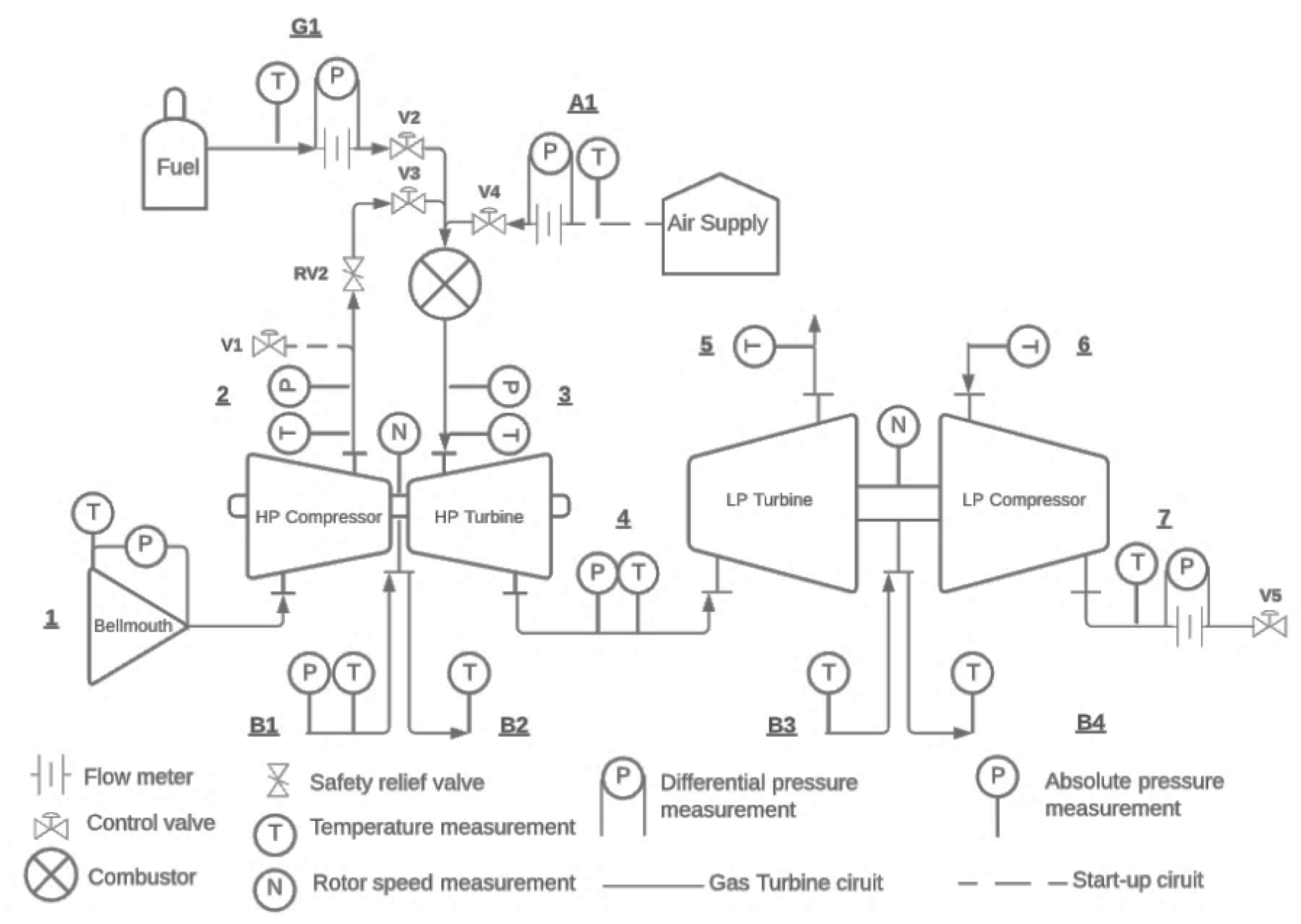
Figure 2.
Left: A sample network of node (i and j) and edges (E1-4). Right: 2-D CFD equivalent with faces (E, S, W and N) and cell centroids (i and j).
Figure 2.
Left: A sample network of node (i and j) and edges (E1-4). Right: 2-D CFD equivalent with faces (E, S, W and N) and cell centroids (i and j).
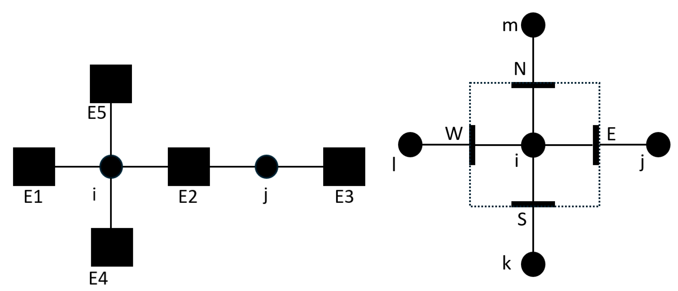
Figure 3.
Section view of the RQL combustor designed by Ssebabi (2020).
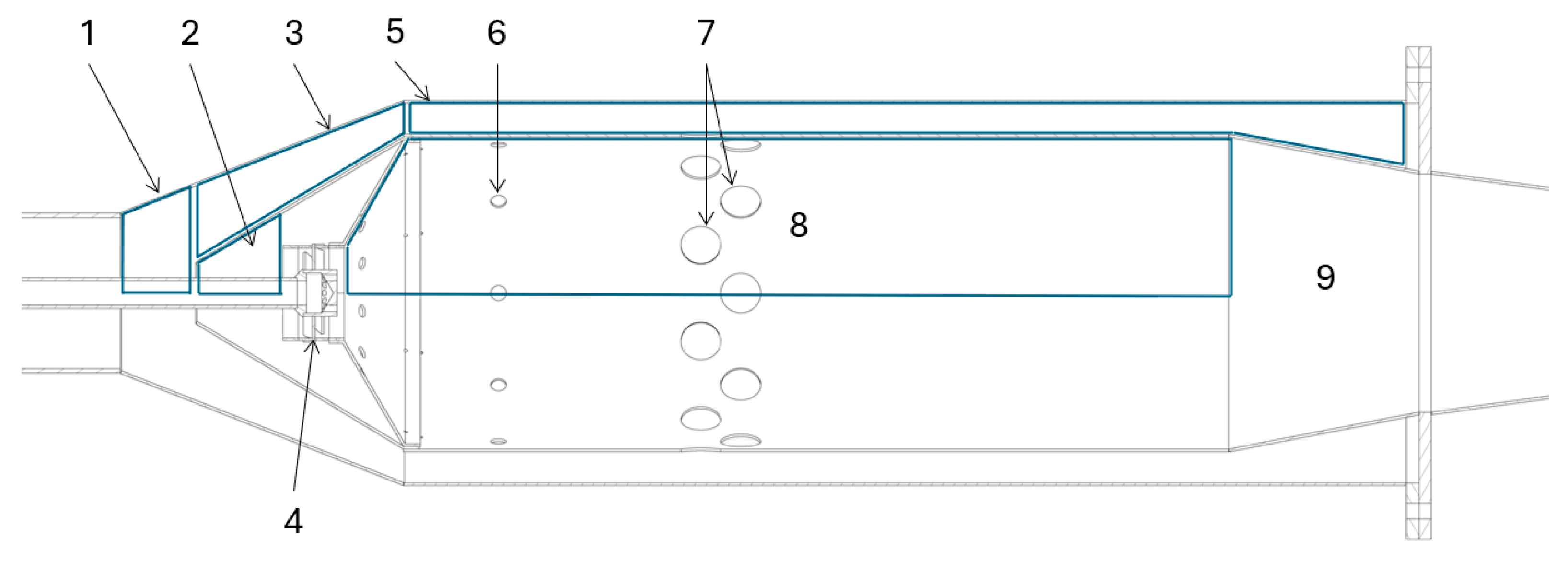
Figure 4.
An illustration of the recirculation flows due to swirl and opposing jets in a RQL combustor.
Figure 4.
An illustration of the recirculation flows due to swirl and opposing jets in a RQL combustor.
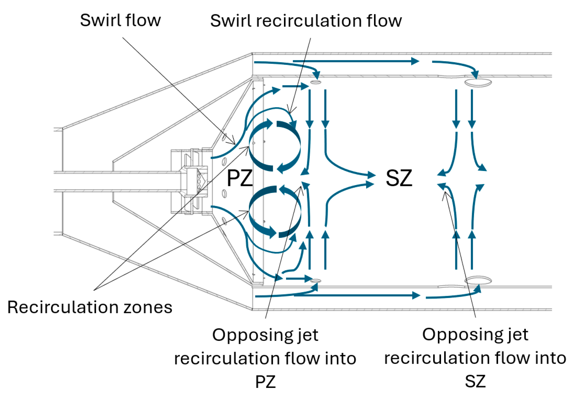
Figure 5.
CFD domain as seen on the y-z plane (top) and an isometric partial section view of the domain highlighting the combustion zones.
Figure 5.
CFD domain as seen on the y-z plane (top) and an isometric partial section view of the domain highlighting the combustion zones.
Figure 6.
Static temperature (left) and velocity magnitude (right) along the combustor’s axis for MGT3.
Figure 6.
Static temperature (left) and velocity magnitude (right) along the combustor’s axis for MGT3.
Figure 7.
Network model of the combustor with reactors and MathCad scripts.
Figure 8.
Pathlines, coloured by velocity magnitude, initiated from the PZ jets (left) and the SZ jets (right) for MGT3.
Figure 8.
Pathlines, coloured by velocity magnitude, initiated from the PZ jets (left) and the SZ jets (right) for MGT3.
Figure 9.
Mass averaged Damköhler number of each combustion zone for varying fuel mixtures of H2 and C3H8.
Figure 9.
Mass averaged Damköhler number of each combustion zone for varying fuel mixtures of H2 and C3H8.
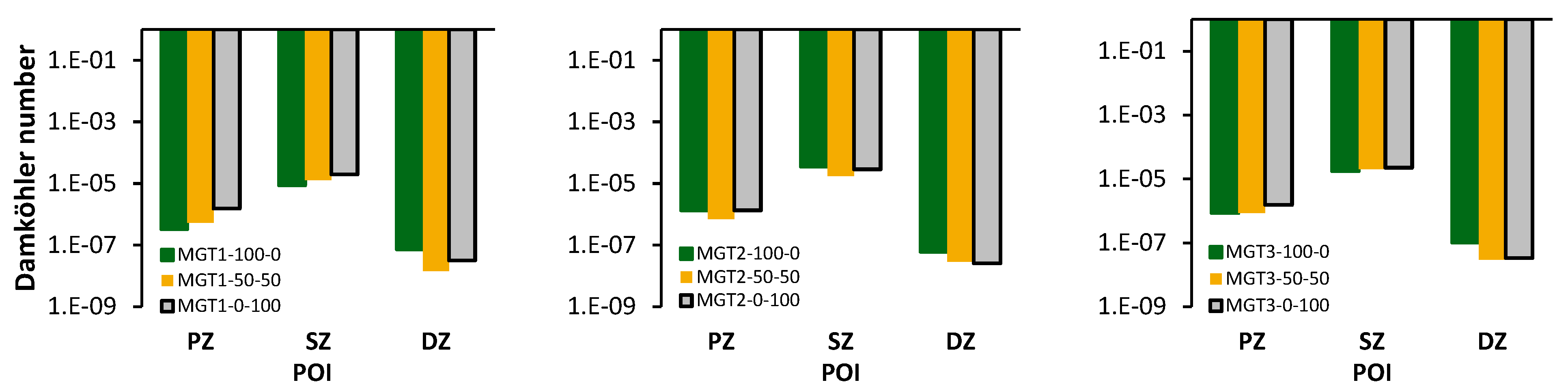
Figure 10.
Combustor performance metrics for each fuel mixture.
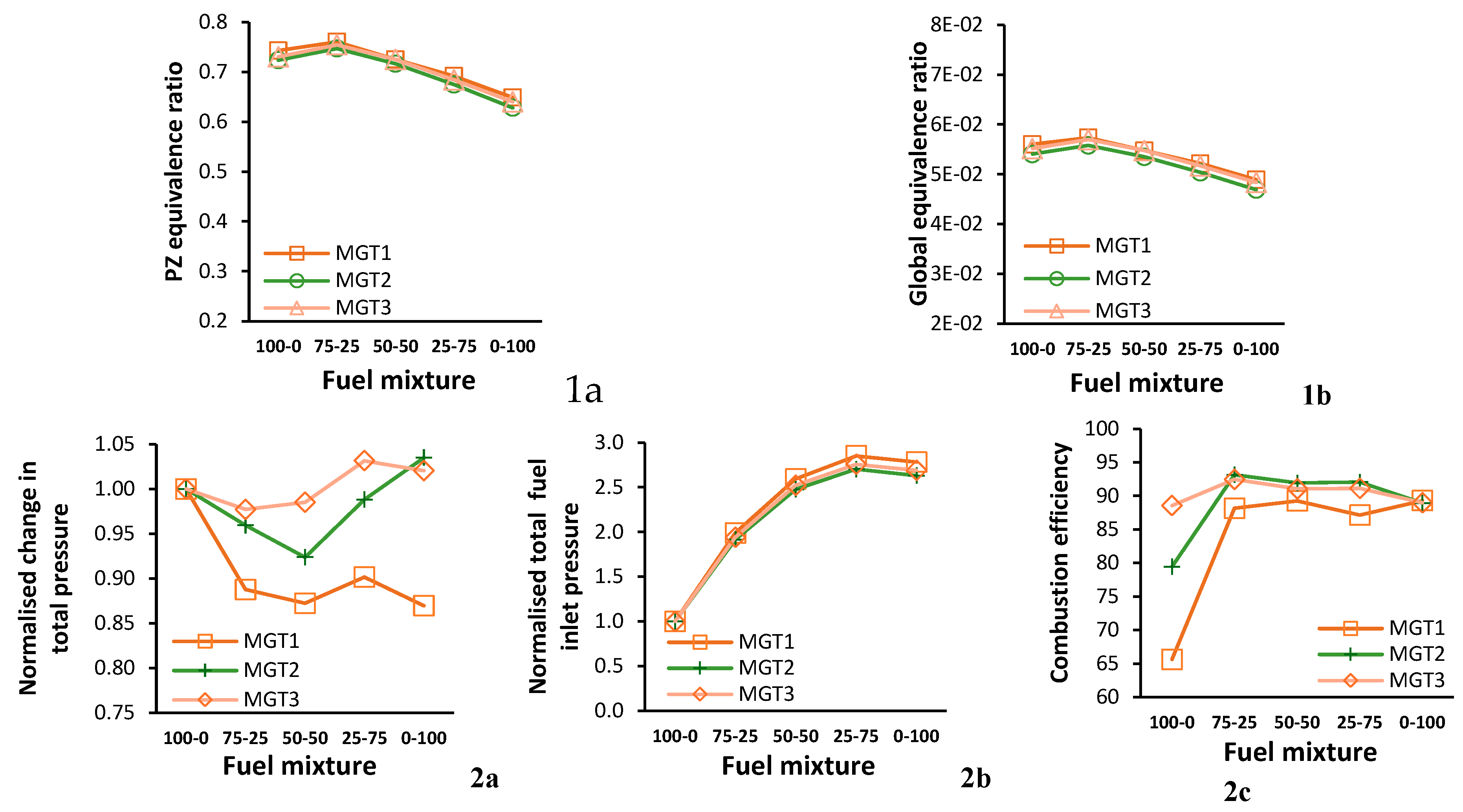
Figure 11.
Spatial variation of key combustion parameters across the planes of combustor zones for different fuel mixtures).
Figure 11.
Spatial variation of key combustion parameters across the planes of combustor zones for different fuel mixtures).
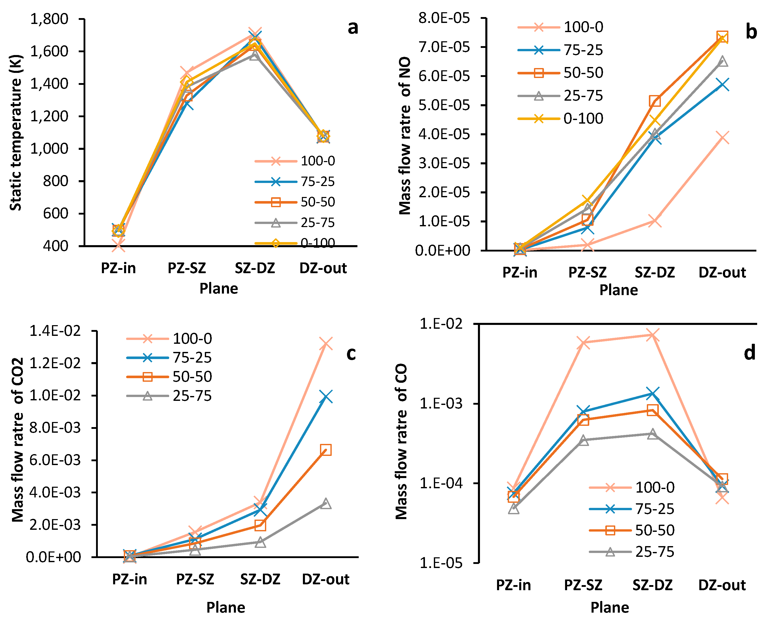
Figure 12.
Combustion zone wall temperature for propane only operation (top), and the wall temperature for mixture fuel operation of each running point (bottom).
Figure 12.
Combustion zone wall temperature for propane only operation (top), and the wall temperature for mixture fuel operation of each running point (bottom).
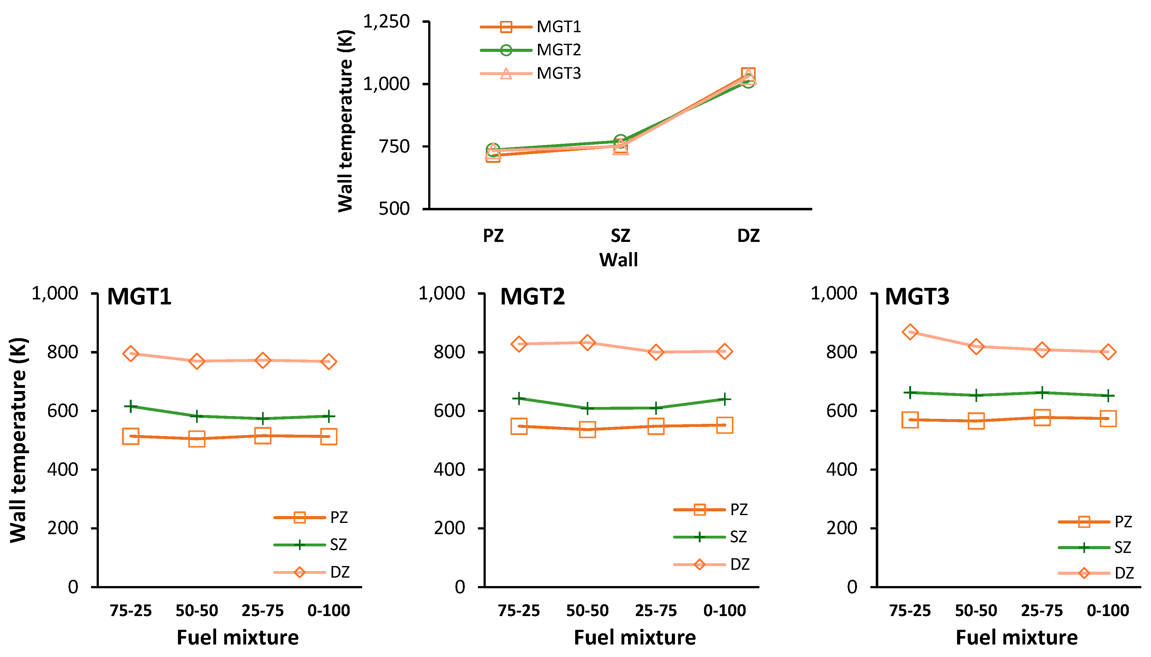
Figure 13.
Static temperature contours for three fuel cases: propane only (left), 50-50 propane-hydrogen mixture (middle), and hydrogen only (right). The dilution zone (DZ) wall region is highlighted by black rectangles.
Figure 13.
Static temperature contours for three fuel cases: propane only (left), 50-50 propane-hydrogen mixture (middle), and hydrogen only (right). The dilution zone (DZ) wall region is highlighted by black rectangles.
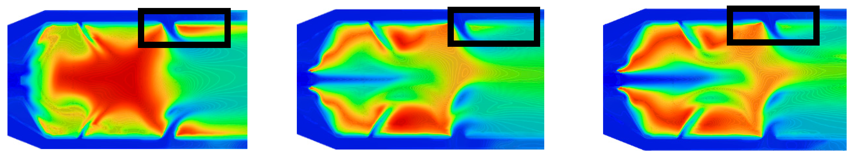
Figure 14.
Network model versus CFD for combustor outlet total temperature and total pressure.
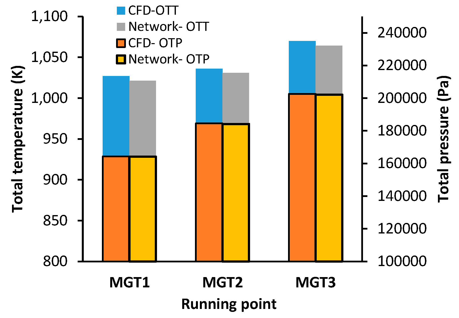
Figure 15.
The change in total pressure across (top) and the mass flow rate through (bottom) each sub-component.
Figure 15.
The change in total pressure across (top) and the mass flow rate through (bottom) each sub-component.
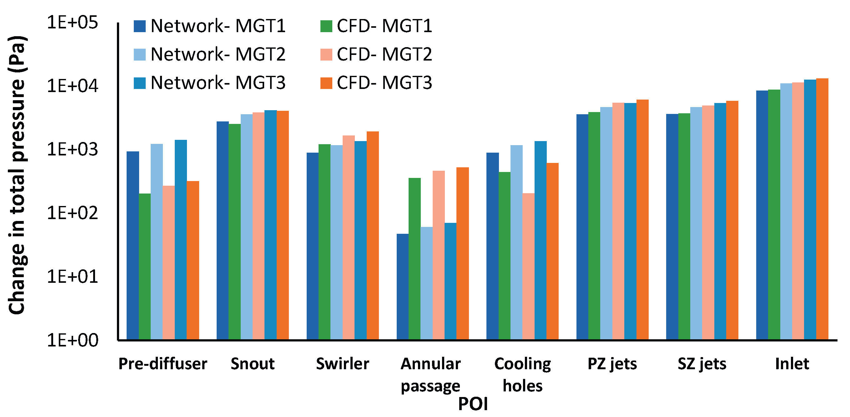
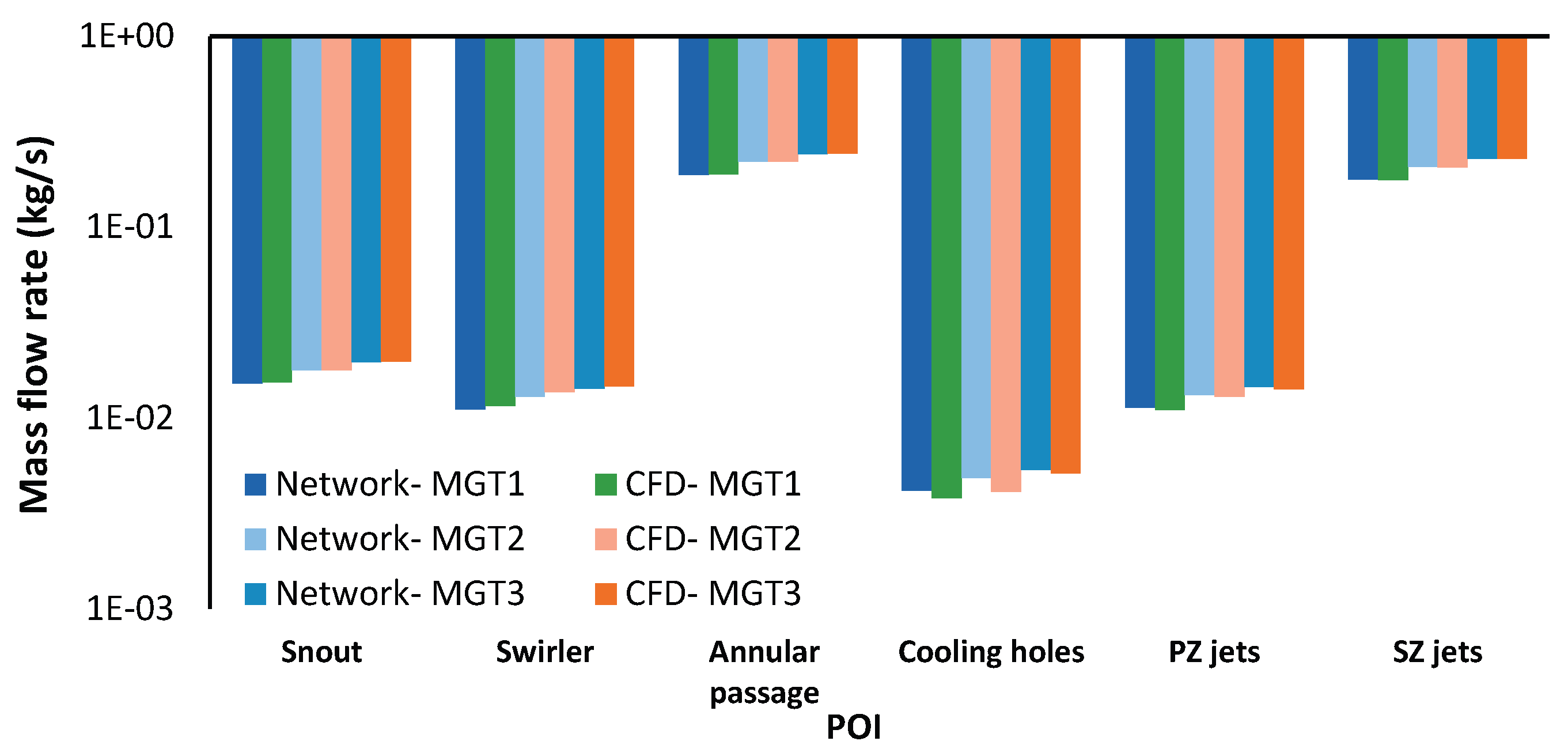
Figure 16.
Combustion zone inner wall temperature (top-left), average combustion zone total temperature (top-right) and the respective relative error (bottom).
Figure 16.
Combustion zone inner wall temperature (top-left), average combustion zone total temperature (top-right) and the respective relative error (bottom).
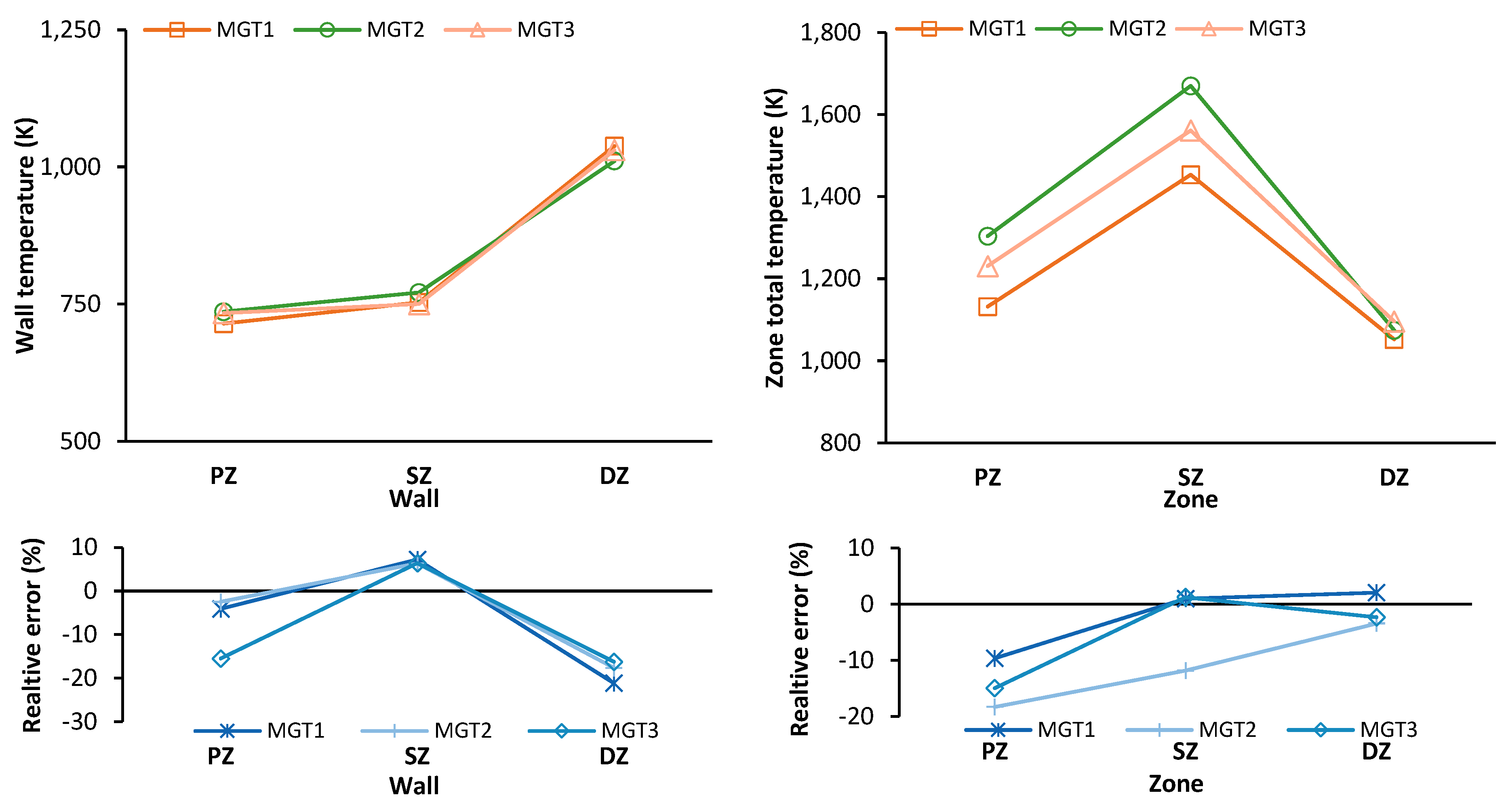
Figure 17.
Outlet CO2 and H2O mass fraction (top left), outlet CO and NO mass fraction (top right). The relative error for CO2 and H2O (bottom left) is also shown together with the normalized CO and NO mass fractions (bottom right).
Figure 17.
Outlet CO2 and H2O mass fraction (top left), outlet CO and NO mass fraction (top right). The relative error for CO2 and H2O (bottom left) is also shown together with the normalized CO and NO mass fractions (bottom right).
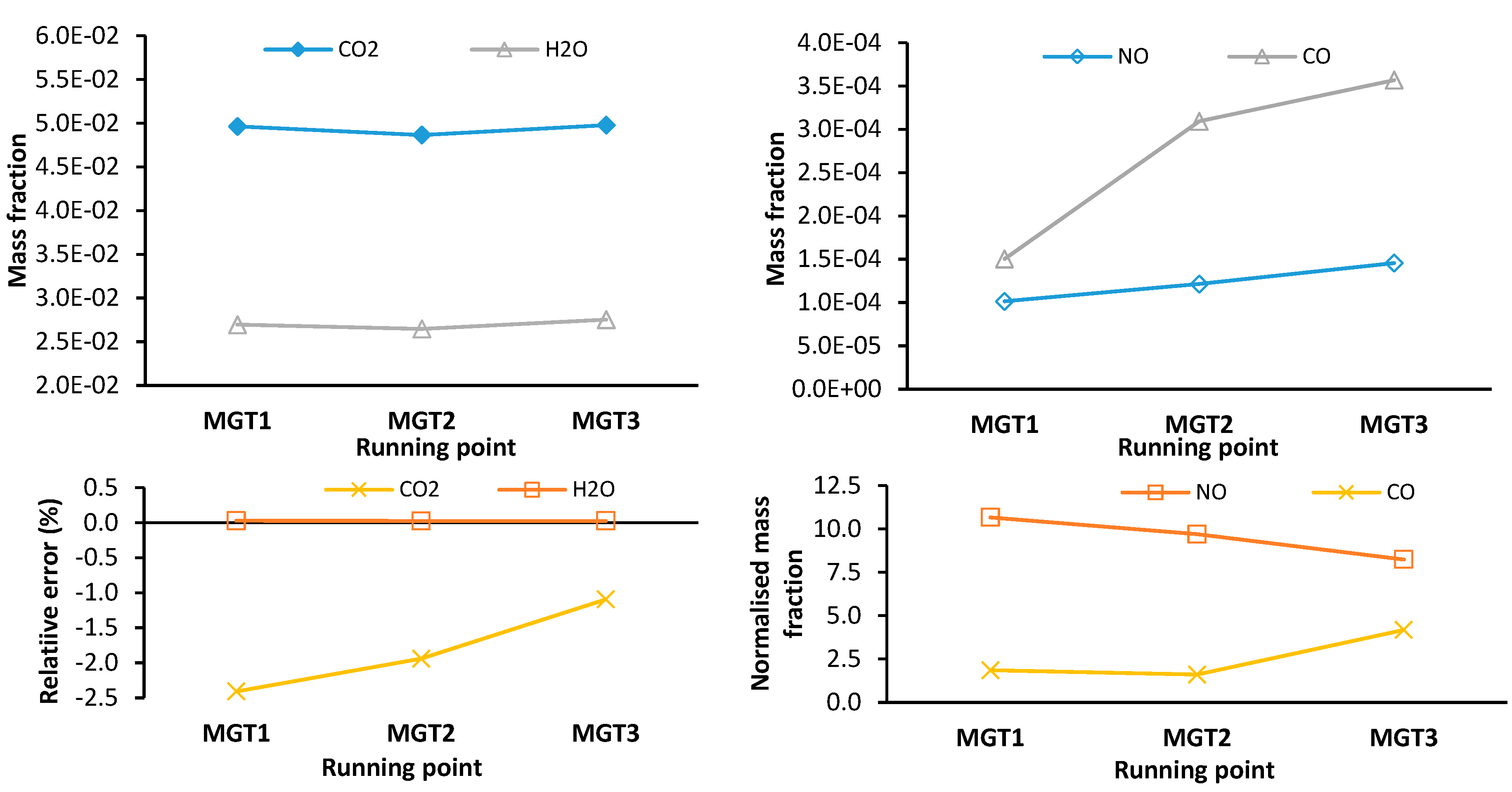
Figure 18.
CFD models outlet total temperature (top left) and the network models relative error (top right). Similarly, the CO2 (middle left) and H2O mass fraction (middle right) with the corresponding relative errors (bottom).
Figure 18.
CFD models outlet total temperature (top left) and the network models relative error (top right). Similarly, the CO2 (middle left) and H2O mass fraction (middle right) with the corresponding relative errors (bottom).
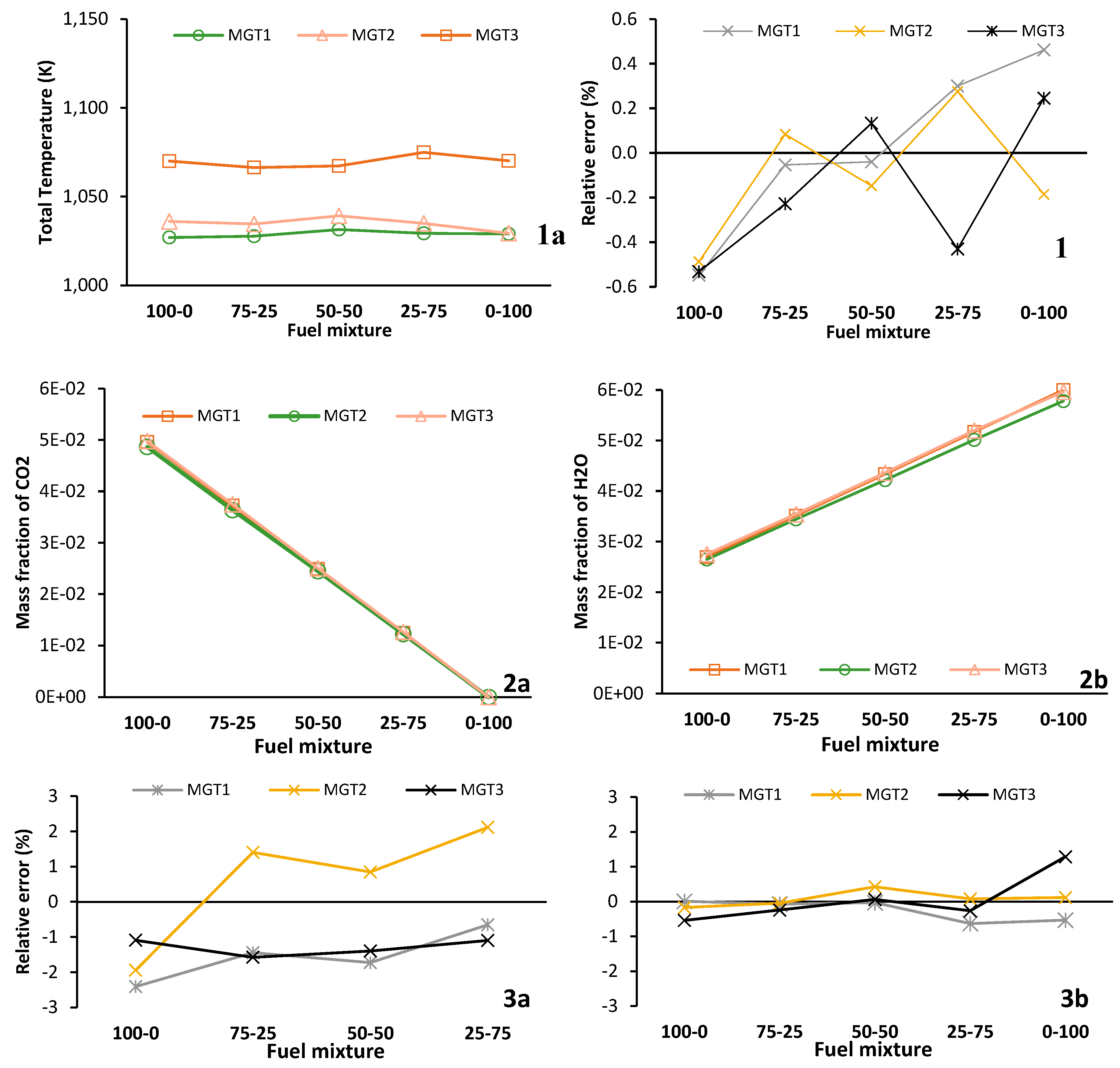
Figure 19.
CO mass fraction (left) and NO mass fraction (right) for varying fuel mixtures of H2 and C3H8.
Figure 19.
CO mass fraction (left) and NO mass fraction (right) for varying fuel mixtures of H2 and C3H8.
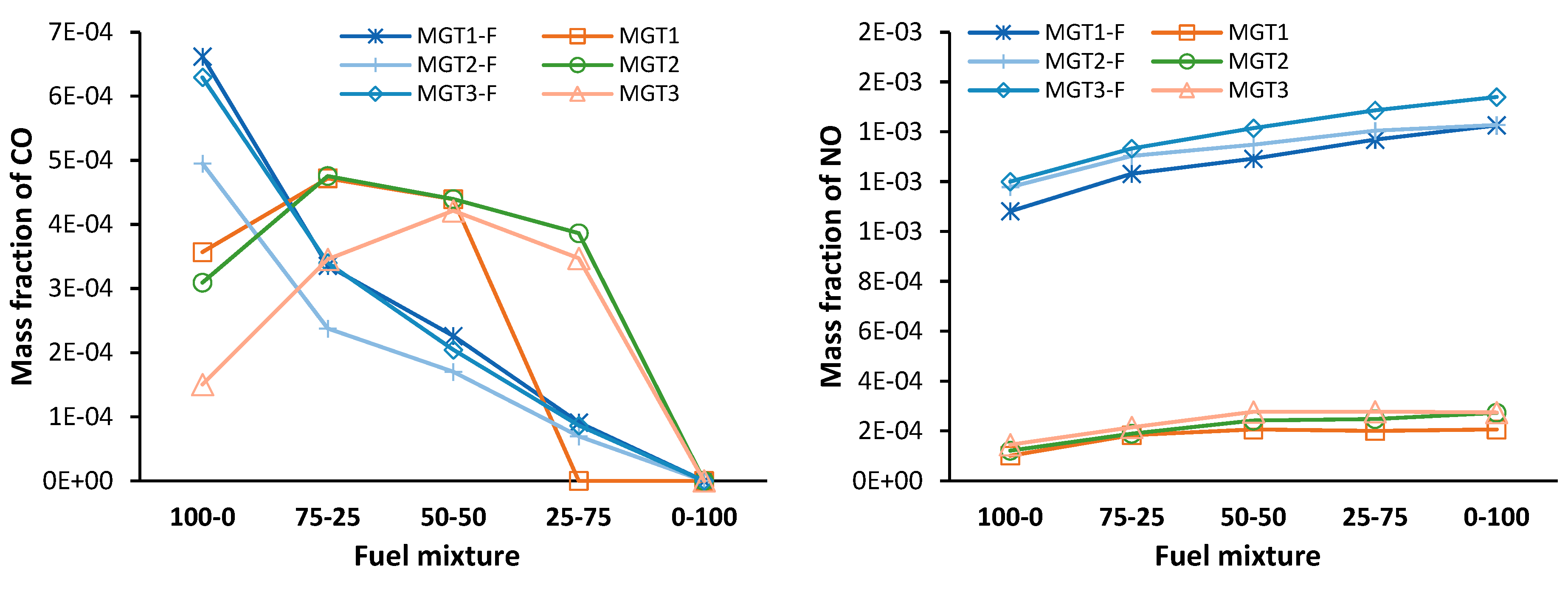
Figure 20.
Absolute zone and wall temperatures for each combustion zone for all blending ratios.
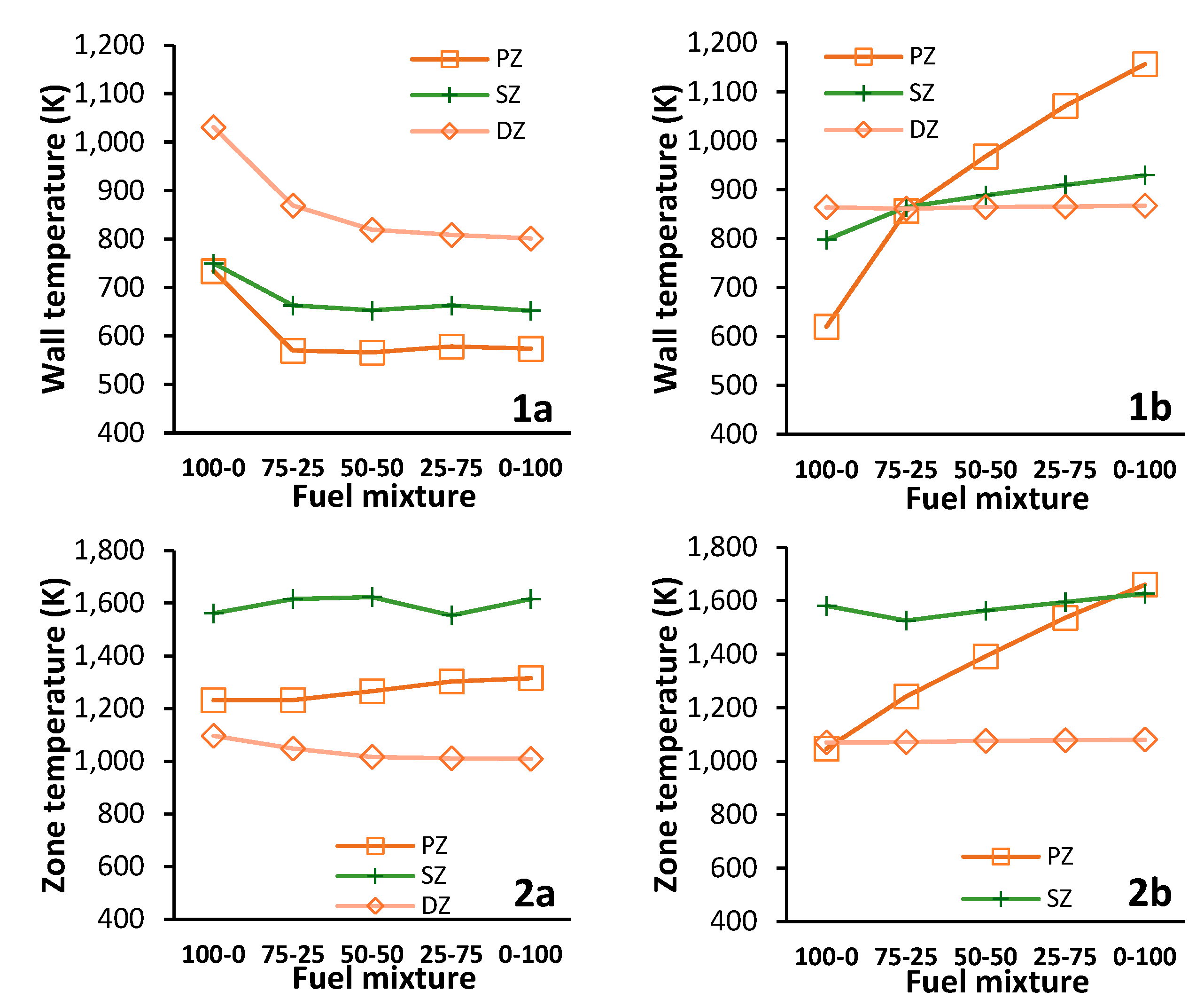

Table 1.
Experimental data from Ssebabi (2020).
|
Case |
Air | Fuel |
Outlet static pressure (kPa) |
|||
|---|---|---|---|---|---|---|
| Mass flow rate (kg/s) | Temperature (K) | Mass flow rate (kg/s) | Temperature (K) | Outlet total temperature (K) | ||
| Station | 1 | 2 | G1 | G1 | 3 | 3 |
| MGT1 | 0.2035 | 351 | 0.0034 | 287 | 155.6 | 1091 |
| MGT2 | 0.2374 | 376 | 0.0039 | 288 | 173.2 | 1121 |
| MGT3 | 0.2614 | 393 | 0.0045 | 289 | 189.5 | 1142 |
Table 2.
Operating conditions for pure hydrogen and pure propane.
|
Case |
Air | Fuel |
Outlet static pressure (kPa) |
||||
|---|---|---|---|---|---|---|---|
| Mass flow rate (kg/s) | Temperature (K) | Mass flow rate H2 (kg/s) | Mass flow rate C3H8 (kg/s) | Temperature (K) | Outlet total temperature (K) | ||
| MGT1 | 0.2035 | 351 | 0.0014 | 0.0034 | 287 | 155.6 | 1027 |
| MGT2 | 0.2374 | 376 | 0.0016 | 0.0039 | 288 | 173.2 | 1030 |
| MGT3 | 0.2614 | 393 | 0.0018 | 0.0045 | 289 | 189.5 | 1070 |
Table 3.
Fuel mixture parameters for each running point.
| Total fuel mass flow rate (kg/s) | Mass fraction | ||||
|---|---|---|---|---|---|
| Mixture | MGT1 | MGT2 | MGT3 | C3H8 | H2 |
| 75-25 | 0.0029 | 0.0033 | 0.0038 | 0.883 | 0.117 |
| 50-50 | 0.0024 | 0.0027 | 0.0031 | 0.714 | 0.286 |
| 25-75 | 0.0019 | 0.0021 | 0.0024 | 0.454 | 0.546 |
Table 4.
Grid Convergence Index parameters.
| Outlet Total Temperature | ||||
| Mesh | φ | Ncells | r | GCI |
| Fine | 1088.71 K | 10526216 | 1.6 | 0.00% |
| Medium | 1089.69 K | 2500099 | 1.3 | 0.11% |
| Coarse | 1105.58 K | 1143823 | ||
| Inlet Total Gauge Pressure | ||||
| Mesh | φ | Ncells | r | GCI |
| Fine | 14368.92 Pa | 10526216 | 1.6 | 0.01% |
| Medium | 14381.83 Pa | 2500099 | 1.3 | 0.12% |
| Coarse | 14435.86 Pa | 1143823 | ||
Table 5.
Total outlet temperature results for the CFD model and experimental data.
| Total outlet temperature (K) | |||
|---|---|---|---|
| Value | MGT1 | MGT2 | MGT3 |
| CFD | 1027 | 1036 | 1070 |
| Experiment | 1091 | 1121 | 1142 |
| Abs error (%) | 5.9 | 7.6 | 6.3 |
Table 6.
Details of the machines used for simulations.
| Simulation | Solver | Location | CPU | # of CPUs | RAM | Average compute time |
| 3-D CFD | ANSYS Fluent V242 | HPC | Intel(R) Xeon(R) E5-2690 v3 | 240 | 1.28TB | approx. 420 minutes |
| 1-D Network | Flownex SE 2022 | Local PC | intel i9-12900K | 1 | 64GB | approx. 1 minute |
Disclaimer/Publisher’s Note: The statements, opinions and data contained in all publications are solely those of the individual author(s) and contributor(s) and not of MDPI and/or the editor(s). MDPI and/or the editor(s) disclaim responsibility for any injury to people or property resulting from any ideas, methods, instructions or products referred to in the content. |
© 2025 by the authors. Licensee MDPI, Basel, Switzerland. This article is an open access article distributed under the terms and conditions of the Creative Commons Attribution (CC BY) license (http://creativecommons.org/licenses/by/4.0/).
Copyright: This open access article is published under a Creative Commons CC BY 4.0 license, which permit the free download, distribution, and reuse, provided that the author and preprint are cited in any reuse.


