Submitted:
28 August 2025
Posted:
28 August 2025
Read the latest preprint version here
Abstract
Marine low clouds have a strong impact on Earth’s system but remain a major source of uncertainty in anthropogenic radiative forcing simulated by general circulation models. This uncertainty arises from incomplete understanding of the many processes controlling their evolution and interactions. A key feature of these clouds is their diverse mesoscale morphologies, which are closely tied to their microphysical and radiative properties but remain difficult to characterize with satellite retrievals and numerical models. Here, we develop and apply a vision–language model (VLM) to classify marine low cloud morphologies using two independent datasets based on Moderate Resolution Imaging Spectroradiometer (MODIS) satellite imagery: (1) mesoscale cellular convection types of sugar, gravel, fish, and flower (SGFF; 8800 total samples), and (2) marine stratocumulus (Sc) types of stratus, closed cells, open cells, and other cells (260 total samples). By conditioning frozen image encoders on descriptive prompts, the VLM leverages multimodal priors learned from large-scale image–text training, making it less sensitive to limited sample size. Results show that the k-fold cross-validation of VLM achieves an overall accuracy of 0.84 for SGFF, comparable to prior deep learning benchmarks for the same cloud types, and retains robust performance under the reduction of SGFF training size. For the Sc dataset, the VLM attains 0.86 accuracy, whereas image-only model is unreliable under such limited training set. These findings highlight the potential of VLMs as efficient and accurate tools for cloud classification under very low samples, offering new opportunities for satellite remote sensing and climate model evaluation.
Keywords:
low clouds
; mesoscale cellular convection
; satellite
; machine learning
; pattern recognition
; vision-language models
1. Introduction
In recent decades, machine learning (ML) models have emerged as a transformative tool in atmospheric science, offering powerful capabilities to untangle complex problems by uncovering nonlinear and high-dimensional relationships [1,2,3]. These capabilities have led to successful applications across a broad range of atmospheric topics, including meteorological prediction, climate processes, aerosol–cloud interactions, and atmospheric chemistry [4,5,6,7]. ML models are increasingly integrated with observations and physical models in various ways, such as ML-driven fusion of air quality modeling and observations [8], development of emulators to accelerate or improve bin microphysics parameterizations in models [9], detection and classification of cloud morphologies from satellite imagery [10], and statistical downscaling of climate model outputs to regional scales [11]. These developments demonstrate the potential of ML as a complementary framework for process-level understanding of different atmospheric phenomena.
Marine low clouds play a key role in Earth’s radiation budget due to their vast coverage and high albedo [12]. Despite this, their contribution to total cloud feedback results in one of the largest uncertainties in anthropogenic radiative forcing [13,14]. This uncertainty arises from the complexity of processes that govern their evolution and from challenges in their representation in general circulation models (GCMs) [15]. With coarse spatial resolution, GCMs are unable to explicitly simulate critical cloud processes such as turbulence, entrainment, and aerosol–cloud interactions [16,17,18]. In contrast, cloud-resolving models are capable of directly simulating these finer-scale processes, but small domain size, short integration time, and sensitivity to background meteorological conditions are among their limitations [19,20,21].
Satellite images show that marine low clouds have a variety of mesoscale morphologies, reflecting different stages of cloud development ranging from stratus in subtropical eastern oceans to organized stratocumulus (Sc; which can appear as open- or closed-cell forms) to shallow cumulus in trade wind regions [12,22]. Each cloud type or morphology is associated with distinct dynamical, microphysical, and radiative properties, evident in variability across static stability, cloud fraction, cloud radiative effect, and precipitation [23,24]. However, conventional remote sensing retrievals of cloud and aerosol properties, derived from radiance at the pixel scale, are not well-suited to differentiate among these cloud morphologies [10]. As a result, visual inspection of satellite images remains a critical step for distinguishing marine low cloud types, highlighting the need for more automated classification frameworks.
Over the past two decades, several studies have classified different types of marine Sc clouds and mesoscale cellular convection (MCC) using traditional deep learning [24] and convolutional neural networks (CNNs) [10,25,26]. CNN classifiers, however, require large, labeled training datasets (typically on the order of thousands of images) to achieve robust performance. Because constructing such datasets in atmospheric science is both costly and labor-intensive, the application of CNNs on cloud classification has remained limited. To address this issue, Geiss et al. (2024) employed a self-supervised neural network, showing that the classification of marine low clouds with this approach is comparable to that of CNNs.
In this study, we address this limitation by introducing a novel approach based on an emerging deep learning framework, the vision–language model (VLM). Unlike CNNs, which rely exclusively on image features, VLMs align images with descriptive text within a shared embedding space [28]. By conditioning frozen image encoders on descriptive prompts, VLMs leverage multimodal priors learned from large-scale image–text datasets, making them far less sensitive to limited sample sizes. This efficiency is particularly advantageous for atmospheric applications, where labeled datasets are often rare. The rest of this paper is organized as follows: Sect. 2 describes the methodology, including data, model framework, training, validation, and evaluation. Sect. 3 presents the results, including model development for SGFF and marine Sc cloud types as well as VLM performance under limited samples. Sect. 4 provides the conclusions.
2. Methodology
2.1. Data
In this study, we develop VLMs for two independent datasets, each representing a widely used framework for categorizing low cloud morphology. First, we employ the satellite images of MCC categories (sugar, gravel, fish, flower, or SGFF) produced by Geiss et al. (2024), which is a processed and quality-controlled subset of the labeled cloud imagery compiled by Rasp et al. (2020). The dataset builds on the cloud regime classification framework of Stevens et al. (2020), who identified four common MCC structures from 900 images in the trade wind region of North Atlantic ocean: 1) sugar (very fine-scale shallow cumulus clouds with little or no organization), gravel (precipitating shallow cumulus cells that are deeper and larger than sugar and form uneven granular pattern), fish (fishbone-like organized cumulus separated from other clouds by cloud-free regions and having the largest size compared to other cell types), and flowers (precipitating organized stratiform clouds appearing as neighboring cells with size comparable to gravel). See Figs. 1-4 in Stevens et al. (2020), Figure 1 in Rasp et al. (2020) and Figure 1 in Geiss et al. (2024) for clear examples of each MCC type.
Rasp et al. (2020) expanded the work of Stevens et al. (2020) and produced 49,000 MCC labels from MODIS Terra and Aqua visible images over three trade wind regions (one in Atlantic and two in Pacific ocean) for a period of 11 years from 2007 to 2017. Geiss et al. (2024) further inspected this dataset and retained only labeled images in which three labelers or more were in agreement on the MCC type. That resulted in a total of 8,800 labeled images with 2,200 samples for each MCC type. They also processed the images to generate uniform 256×256-pixel resolution suitable for machine learning applications.
Second, we constructed a labeled dataset focused on marine stratocumulus (Sc) clouds predominant over subtropical ocean basins. Three key regions were selected based on persistent Sc cover: the subtropical Northeast Pacific, the subtropical Southeast Pacific, and the subtropical Southeast Atlantic. The satellite imagery used in this analysis is acquired from the Moderate Resolution Imaging Spectroradiometer (MODIS) aboard the polar-orbiting Aqua and Terra satellites [29]. MODIS provides coverage with two daytime passes (one from each satellite) for each location on earth. We utilize Level-1B true-color (red–green–blue or RGB) reflectance, with spatial resolution ranging from 250 m to 1000 m depending on the spectral band and viewing geometry. These images are accessed through NASA Worldview.
Scenes are extracted from May to September over a 10-year period (2015–2024), targeting daylight visible images with minimal sun-glint contamination to preserve image quality and contrast among cloud structures. We also exclude scenes from the edges of images, which tend to exhibit geometric distortion and stretching, and select scenes predominantly over ocean and free from high-level clouds. All images have a resolution of 256 × 256 pixels to be consistent with the SGFF dataset format and to match the patching strategy of our VLM. Four types of Sc clouds are considered, with 65 samples labeled for each type, yielding a total of 260 hand-labeled images. The categories are (Figure 1): stratus clouds (smooth, featureless layers of low clouds with horizontal development), closed cells (puffy, bright cells surrounded by narrow dark edges forming capped honeycomb structures), open cells (bright cloud rings surrounding dark, cloud-free centers forming honeycomb-like patterns), and other cells (disorganized or broken cellular clouds appearing as patches or fragments). This classification follows prior studies on marine Sc cloud morphology [10,23,24], although some have adopted slightly different numbers or definitions of Sc cloud types depending on the region of study and availability of samples for each cloud type.
2.2. Model Framework
The classification technique in this study is based on OpenCLIP [30], an open-source implementation of the Contrastive Language–Image Pretraining (CLIP) model [28]. CLIP uses a dual-encoder transformer architecture, consisting of a vision encoder and a text encoder that project image and text representations into a shared embedding space in order to associate semantic concepts with visual patterns (Figure 2). The model is trained using a contrastive loss function that maximizes the cosine similarity between matched image–text pairs while minimizing similarity between mismatched pairs.
In our configuration, the vision encoder is a Vision Transformer (ViT-B/32) architecture [31], which processes non-overlapping 32×32-pixel patches from each 256×256 image and embeds them into a fixed-dimensional representation ( in Figure 2). The text encoder is a transformer-based language model that encodes short natural-language descriptions of cloud categories into the same embedding space ( in Figure 2). Both encoders output 512-element vectors (1-D embeddings), which are then normalized and passed to a projection head for similarity computation.
In this study, we freeze all weights of the pretrained vision and text encoders and fine-tune only the projection head. Each projection head is parameterized by a 512×512-element weight matrix ( for images, for text) that linearly transforms the encoder outputs into a shared multimodal embedding space (represented by for images and for text in Figure 2). The cosine similarity between all and pairs forms a similarity matrix S, where each element quantifies the alignment between image i and text j. This similarity matrix is used in the symmetric cross-entropy contrastive loss, which encourages matched image–text pairs to have high similarity and mismatched pairs to have low similarity. Freezing the encoders while training only and is a common transfer learning strategy that reduces computational cost [32,33] and mitigates overfitting when working with relatively small, domain-specific datasets [34,35]. This choice preserves the general visual–prompt knowledge obtained during large-scale pretraining of OpenCLIP (involving hundreds of millions of publicly available image–text pairs) while adapting the model to specialized datasets focused on a narrow range of image types, in this case, satellite imagery of marine Sc clouds and MCC morphologies.
For prompt engineering, we use descriptive phrases corresponding to the cloud morphological types of the two datasets, namely MCCs (sugar, gravel, fish, and flower) and marine Sc clouds (stratus, closed cells, open cells, and other cells), as described in Sect. 2.1. Each phrase emphasizes distinctive morphological features identifiable in visible MODIS true-color imagery. These text prompts serve as conditioning inputs to the text encoder during inference, providing a semantic anchor for each cloud type. To enhance robustness, we employ an ensemble prompting strategy, in which multiple prompts for each category are created through variations in wording, synonyms, or sentence structure, and their similarity scores are averaged. Prompt-ensemble strategies in VLMs have been shown to produce slightly higher accuracy compared to using a single prompt per class [28,36].
2.3. Training Procedure
Training is conducted using the AdamW optimizer [37] with a learning rate of 5 × 10⁻⁵ and a weight decay of 1 × 10⁻⁴, settings commonly adopted for fine-tuning large pretrained models on smaller, specialized datasets to balance convergence speed and stability. The learning rate is deliberately small to avoid catastrophic forgetting of pretrained visual–text representations while allowing gradual adaptation to the target cloud-classification tasks [32,38]. Weight decay regularizes the projection head and mitigates overfitting without overly constraining the learned weights [39]. Training is run for 50 epochs, which allows convergence under these low learning-rate settings while avoiding unnecessary computation and overfitting.
The loss function is the symmetric cross-entropy contrastive loss used in CLIP-type models, which simultaneously maximizes similarity between matched image–text pairs and minimizes similarity between mismatched pairs in order to improve bidirectional retrieval and representation alignment in the joint embedding space [28,40]. A cosine learning-rate schedule with warm restarts [37,41] is applied, smoothly decaying the rate within each cycle and periodically resetting it to escape shallow minima and improve generalization.
The model is implemented in PyTorch [42], and all training and inference processes are executed on CPU hardware, as the dataset sizes and model architecture make GPU acceleration unnecessary for achieving acceptable runtimes. We vary batch sizes by dataset size and processing stage to balance convergence stability with computational efficiency on CPU hardware, consistent with previous studies on batch size selection [43,44]. For the SGFF dataset (8,800 images), we use a batch size of 64 when extracting frozen image embeddings and 128 when fine-tuning the projection head on frozen embeddings. For the marine Sc dataset (260 images), batch sizes are 16 for extraction of the frozen embedding and 32 for during the projection head fine-tuning. These batch sizes follow standard practice in VLM fine-tuning. In the early embedding extraction step, we use smaller batches to reduce CPU memory usage. In the later fine-tuning step, we increase the batch size to make model updates more stable and improve training efficiency [45].
2.4. Testing the Model and Cross-Validation Strategy
To test the model results, we utilize a k-fold cross-validation approach [46,47,48], which is widely used to assess the generalization capability of machine learning models and reduce overfitting. In this framework, the labeled dataset is randomly divided into k equally sized and mutually exclusive subsets. In our analysis, we set k = 5. For each iteration, one subset is held out as an independent test set, while the remaining k – 1 subset are combined to form the training set. The model is trained on this training set and subsequently evaluated on the held-out subset to provide an estimate of its predictive skill on data not seen during training. This process is repeated k times, with each subset serving as the test set exactly once. Once all k iterations are completed, predictions from each test subset are concatenated to form a complete set of model outputs from the entire dataset. The repeated training–testing cycle reduces the likelihood of overfitting to a particular subset of the data and provides a more reliable measure of performance than a single train–test split. Evaluation metrics are then computed across the aggregated prediction set.
2.5. Evaluation Metrics
To quantify the performance of the VLM, we compute a standard set of evaluation metrics commonly used in multi-class classification tasks: accuracy, precision, recall, and F1-score [49]. Because the dataset is balanced across classes, we calculate metrics for each class individually and then average across classes (macro-average technique). Here, a short description of each metric is provided [47,50]. For each class, precision () is defined as:
where is the number of true positive for class i, and is the number of false positive for class i. reflects the model’s ability to avoid false alarms, that is, what fraction of the predicted instances of a given class were actually correct. Another metric is recall (), also known as sensitivity or true positive rate, which is defined for each class as:
where is the number of false negative for class i. shows correctly identified samples out of all actual samples of class i. To balances the trade-off between precision and recall, F1-score is defined as the harmonic mean of these two metrics for each class:
F1-score is particularly useful when assessing performance on classes that are underrepresented. Thereafter, the macro-averaged metrics are calculated as:
and similar equations for R and F1. Here, c is the number of classes. Lastly, accuracy (A) can be defined as:
where N is the total number of samples. It represents the proportion of all correctly classified samples out of the total number of samples, regardless of class.
In addition, we present confusion matrices to visualize the distribution of correct and incorrect predictions across both the four MCC categories (SGFF) and the marine Sc types (SCOO). The diagonal elements of the matrix represent correct predictions for each class, while the off-diagonal elements correspond to incorrect predictions. This allows identification of systematic misclassification patterns [50].
3. Results
3.1. Model Development for SGFF Cloud Types
Two configurations of the VLM are developed for the MCC classification: image–only and prompt–image. In the image–only configuration, the text encoder is omitted, and training operates solely on the visualization. Images are first processed by the frozen image encoder to produce 512-element embeddings (), which are then passed through the fine-tuned projection head () to yield projected vectors (). A cosine similarity matrix is computed between projected embeddings in a batch, and a supervised (or image–image) contrastive loss [51] is applied in order to encourage samples of the same class to be close in the embedding space while pushing apart samples from different classes. This setup is conceptually similar to single-modality contrastive representation learning frameworks [52], but with a frozen pretrained encoder and fine-tuned projection head for efficient transfer learning [34]. In the prompt–image configuration, both image and text embeddings ( and ) are generated by their respective frozen encoders, projected via and into a shared space ( and ), and normalized. Cosine similarities are then computed across modalities, and the symmetric cross-entropy contrastive loss used in CLIP-type models [28] is applied to align paired image–prompt representations while separating mismatched pairs. While the prompt–image setup is our main purpose, the image–only model is included as a baseline to quantify the added benefit of prompt conditioning in enhancing the accuracy of classification.
The performance of the developed VLMs for both image–only and prompt–image configurations is summarized in Table 1, with all metrics calculated from 5-fold cross-validation. For the image–only configuration, macro-averaged precision, recall, F1-score, and overall accuracy are all approximately 0.72. Across MCC types, evaluation metrics vary by more than 20%. The sugar class exhibits the highest F1-score (0.782), reflecting a balance between relatively high precision (0.827) and recall (0.743). The flower class achieves the highest recall (0.851) but, with lower precision (0.672), attains the second-highest F1-score (0.751). In contrast, the fish class shows the lowest F1-score (0.644), stemming from both the lowest recall (0.625) and precision (0.664), indicating a higher rate of misclassification. The confusion matrices are shown in Figure 3, where values are normalized by the number of samples in each true class; thus, the diagonal elements correspond to the recall values in Table 1, and the off-diagonal elements represent misclassifications. For the image-only configuration, fish type is most often incorrectly predicted as flower (26.5%) or gravel (7.8%), while sugar is misclassified as gravel (16.7%) and, flower is misclassified as fish (13.8%). The wrong prediction of gravel is more evenly distributed among the other classes, averaging about 12% each.
Incorporating prompt–image projection substantially improves classification skill on average and across all four classes. The macro-averaged precision, recall, and F1-score, along with overall accuracy, are all 0.838, representing a 12% increase compared to the image–only configuration. All evaluation metrics have improved across all classes. From Table 1, sugar class achieves the highest F1-score (0.875) and fish the lowest (0.784). The highest precision is obtained for sugar (0.877), while the highest recall is for flower (0.886). Gains are most pronounced in classes that previously had the lowest evaluation metrics under the image–only configuration: F1-score increases by approximately 15%, 14%, 11%, and 9% for gravel, fish, flower, and sugar, respectively. Precision improves the most for flower (+17%), while recall improves the most for gravel (+17%). By contrast, precision in sugar and recall in flower increase by only 5% and 4%, respectively. The confusion matrix (Figure 3) shows that most off-diagonal misclassifications are reduced, with the strongest errors nearly halved. For example, in the prompt–image configuration, fish is misclassified as flower in 13.5%, sugar is misclassified as gravel in 8.5%, and flower is misclassified as fish in 9.1% of cases.
These results demonstrate that integrating prompt–image projection within the VLM framework enhances MCC classification ability, particularly for classes with high intra-class variability. Overall, our findings are consistent with those of Geiss et al. (2024). A direct comparison, however, is not straightforward, because their study employed a single train–test split for validation, whereas we use k-fold cross-validation, which typically yields lower but more reliable performance estimates (since it averages over multiple random splits and avoids sampling bias). Nevertheless, the accuracy of our prompt–image configuration falls within the range of values (0.829 to 0.877) reported by Geiss et al. (2024) for multiple supervised and self-supervised neural networks applied to SGFF. In addition, their confusion matrix shows best performance for sugar and worst for fish, consistent with our findings, and the patterns of misclassification across classes are also very similar to those we report.
3.2. VLM Performance Under Limited Samples
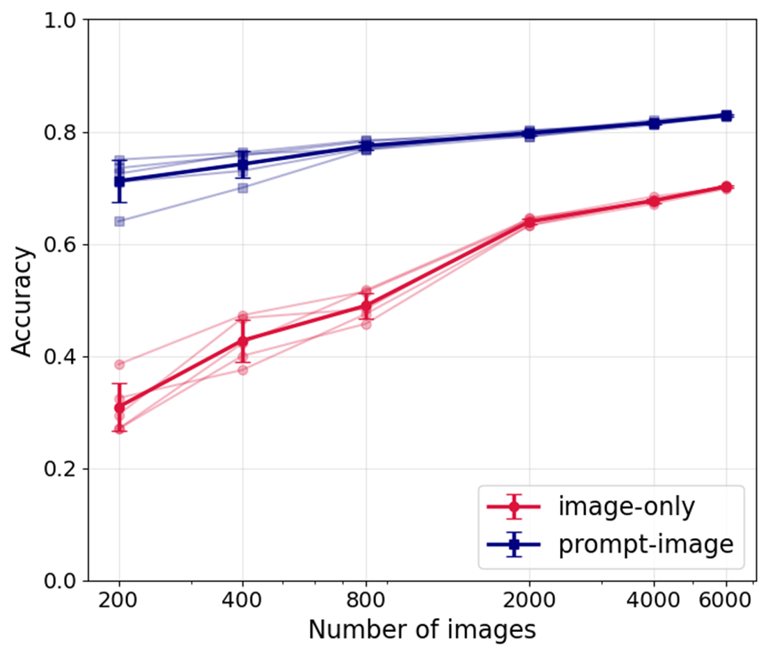
To evaluate the robustness of our approach under limited training data, we compare the performance of an image-only configuration with the prompt–image projection across progressively smaller subsets of the SGFF dataset. We select target sample sizes of 6000, 4000, 2000, 800, 400, and 200, and for each size, we randomly draw five independent subsamples from the full dataset (8800 samples) to account for variability in sample composition. Each subsample is used to train the respective model configuration, and classification accuracy is estimated using k-fold cross-validation. This procedure ensures that the reported performance does not depend on a single random draw of training cases but instead reflects more general behavior across multiple realizations.
Although built atop pretrained embeddings, the image-only model shows strong sensitivity to dataset size: the average accuracy is 0.70 for a sample size of 6000 and it reduces progressively with sample size, declining rapidly when fewer than ~1000 images are available and reaching ~0.31 for 200 samples (Figure 4). This behavior is consistent with broader findings across the machine learning literature. Deep neural networks applied to subsampled benchmarks exhibit significant performance loss when the number of training images is reduced [53,54]. In earth science and remote sensing, traditional machine learning and neural network image classifiers likewise show strong sensitivity to dataset size, with accuracy declining sharply as the number of labeled samples decreases [55,56]. These collective results confirm that image-only approaches are highly dependent on labeled sample size, further motivating the need for alternative strategies such as VLMs.
In contrast, the prompt–image projection maintains substantially higher accuracy across all sample sizes, from 0.83 at 6000 samples down to only 0.71 at 200 samples. This demonstrates the data efficiency gained by conditioning the frozen image encoder on descriptive prompts. Such robustness aligns with recent findings using CLIP-based models, which show that prompt tuning enables strong generalization and achieves high skill even in limited-data regimes [57,58,59]. By leveraging the multimodal prior encoded in their pretrained joint image–text space, VLMs are far less dependent on large, labeled datasets and therefore remain resilient in settings where conventional neural networks break down.
This finding is particularly relevant for application to our Sc cloud dataset, where the total number of available labeled images is only 260. By showing that the reduction in sample size has minimal impact on the VLM’s performance relative to the image-only setup, we establish that our approach remains viable for datasets of this scale, thereby motivating the analysis of Sc morphologies presented in the next sub-section.
3.3. Model Development for Marine Sc Cloud Types
Following the general evaluation of model robustness under different training sample sizes, we now apply the two model configurations to the classification of marine Sc cloud morphologies. With only 260 labeled images, this dataset provides a test of VLM feasibility when training samples are highly limited. Such a scenario is common in atmospheric science, where the construction of labeled cloud datasets requires significant manual effort and often cannot match the scale of benchmark datasets available in computer vision.
Table 2 summarizes evaluation metrics after five-fold cross-validation. The image-only configuration shows significant limitations when applied to this dataset, with the overall accuracy and macro-averaged precision, recall, and F1-score values of approximately 0.4. At the class level, performance varies substantially. F1-scores range from 0.247 for open cells to 0.504 for other cells. Open cells are the most problematic class: precision is only 0.375 and recall falls to 0.185, meaning that the majority of open-cell cases are misclassified. Other cells achieve the highest relative performance, with precision of 0.516 and recall of 0.492. Considering that the probability of correct classification by random chance is 0.25, these results indicate that most classes achieve only marginal improvement over guessing. The confusion matrix further highlights this issue since the distributions of predictions are broadly spread across off-diagonal elements (Figure 4). Open cells are more often misclassified as closed cells (38.5%) than identified correctly (18.5%), while stratus is most frequently misclassified as closed cells (35.4% compared to 47.7% correct). These patterns reflect the sensitivity analysis in Section 3.2, where image-only models degrade sharply when the training set is reduced below 1000 samples.
Figure 4.
As in Figure 2, but for marine Sc cloud category.
Figure 4.
As in Figure 2, but for marine Sc cloud category.
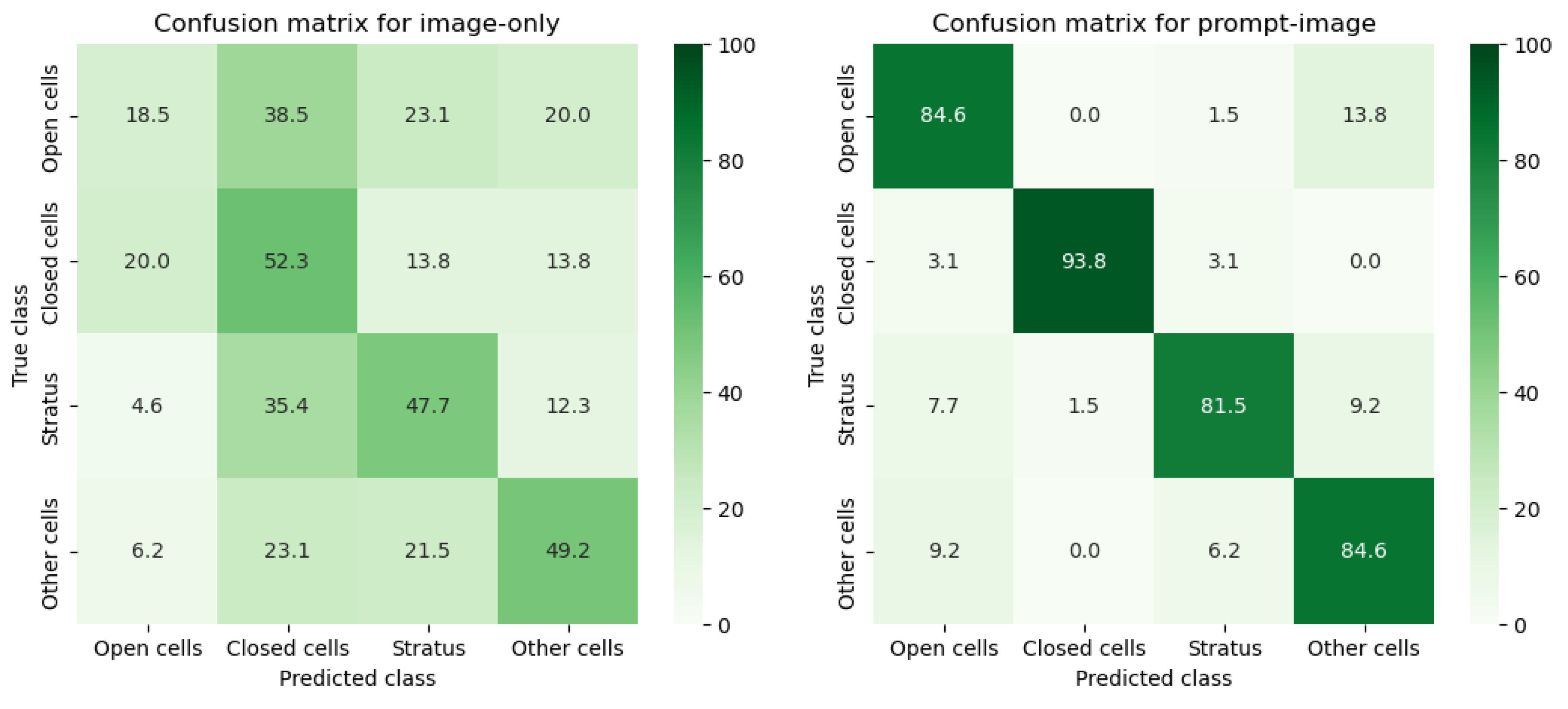
In contrast, the prompt–image projection delivers a remarkable improvement across all evaluation metrics. The overall accuracy and macro-averaged precision, recall, and F1-score increase to approximately 0.86 (Table 2). Each class achieves robust performance, with F1-scores of 0.961 for closed cells, 0.848 for stratus, 0.827 for open cells, and 0.815 for other cells. Closed cells stand out, with precision of 0.984 and recall of 0.938, yielding the highest skill among all categories. The corresponding confusion matrix (Figure 4) reveals that most samples align along the diagonal, with minimal misclassification. Closed cells are identified with the greatest accuracy, with 6.2% of samples misclassified as either open cells or stratus. Open cells are most often misclassified as other cells (13.8%), stratus is more frequently mis-predicted as other cells (9.2%), and other cells are misclassified most often as open cells (9.2%).
These findings provide further validation of the results identified in Section 3.2. While the image-only configuration collapses when training data are reduced below a thousand samples, the prompt–image approach demonstrates resilience even when fewer than 300 labeled images are available. More broadly, the results illustrate the potential of VLMs for remote sensing and cloud physics applications, where large, annotated training datasets are often scarce and challenging to create.
Comparison with prior studies further emphasizes this advantage. Previous efforts to classify marine low cloud imagery have relied on traditional machine learning or image-only neural networks, which perform well when thousands of labeled samples are available [10,23,24]. Geiss et al. (2024) used approximately 2500 labeled samples of marine Sc clouds based on the dataset of Yuan et al. (2020) and evaluated various supervised and self-supervised neural networks. Their reported accuracy values ranged between 0.741 and 0.824, which were 0.033–0.090 lower than the same models applied to the SGFF dataset with 8800 labeled samples. They attributed this decrease in skill to the limited sample size of the Sc dataset. Our results align with this interpretation: dataset size imposes a strong limitation on image-only models. However, VLMs provide an effective alternative, achieving levels of skill that are unattainable for conventional image-only models when only limited labeled data are available for training.
4. Conclusions
Marine low clouds exert a strong effect on Earth’s radiative balance but remain a major source of uncertainty in anthropogenic climate forcing. A key challenge lies in their diverse mesoscale morphologies, which are associated with dynamical and physical properties but remain difficult to distinguish using conventional satellite retrievals. Previous studies applied neural networks to satellite imagery for low cloud classification [10,24,25,26], but a primary limitation of such deep learning methods is their dependence on very large labeled datasets. One way to mitigate this constraint is through self-supervised learning [27]. Alternatively, this study develops a vision–language model (VLM) framework using OpenCLIP [28] for classifying marine low cloud morphologies, demonstrating its potential to perform accurately even with very small sample sizes.
The VLM is built on a frozen image encoder pretrained on large-scale image–text data, coupled with a linear projection head fine-tuned using descriptive language prompts. This architecture aligns images and text within a shared embedding space, allowing classification to be guided by semantic descriptions of cloud types rather than relying solely on image features. Two independent datasets are used to evaluate performance: the MCC SGFF categories (8800 labeled MODIS scenes) and marine Sc morphologies (260 labeled MODIS scenes). To achieve robustness, we use k-fold cross-validation and then calculate evaluation metrics.
For the SGFF dataset, the VLM achieves balanced performance across all four classes, with overall accuracy, precision, recall, and F1-score of 0.84, representing a 12% gain over the image-only baseline. Improvements in VLM are strongest for classes that are typically most challenging in image-only configuration (fish and gravel). Confusion matrix analysis confirms that off-diagonal errors are reduced, with major misclassifications nearly halved relative to the image-only model. Accuracy is comparable to previous CNN-based benchmarks [27]. Additional sensitivity tests reveal that the image-only configuration is strongly dependent on training size, with accuracy declining from 0.70 at 6000 samples to 0.31 at 200 samples. By contrast, the VLM maintains substantially higher accuracy across all sample sizes, from 0.83 at 6000 samples to 0.71 at 200 samples. This demonstrates the efficiency gained by conditioning frozen encoders on descriptive prompts and highlights the resilience of the approach in small-sample regimes, consistent with findings from CLIP-based studies in computer vision [59].
For the Sc dataset of only 260 labeled images, the contrast between the two model configurations is pronounced. The image-only model produces unreliable classifications, with overall accuracy of 0.419 and class-based performance skills ranging from 0.19 to 0.52. In contrast, the VLM achieves balanced accuracy, precision, recall, and F1-score of 0.86, with class-level performance ranging from 0.79 to 0.98. These results confirm that VLMs are far less dependent on large, labeled datasets, enabling high skills even in very limited datasets.
An additional strength of this approach is its computational efficiency. Because the backbone remains frozen and only a linear projection head is fine-tuned, the VLM can be trained and run effectively on CPUs without requiring specialized GPUs. This lowers the barrier for applying advanced deep learning methods in atmospheric research, making VLMs both accurate and accessible for researchers with limited computational resources.
It is worth mentioning several limitations and suggestions. Future work could explore fine-tuning both the image encoder and language prompts. though this could increase computational cost. Performance may also depend on hyperparameters such as prompt design, learning rate, weight decay, and model architecture, which should be systematically tested. Moreover, expanding the framework to other datasets, regions, and time periods will be essential for assessing generalizability. Last but not least, as noted by Yuan et al. (2020), another source of uncertainty in cloud classification is that even expert humans might classify the same satellite image differently, and this ambiguity must be accounted for when evaluating automated systems.
Despite these limitations, our results demonstrate that VLMs provide a reliable, data-efficient, and computationally inexpensive framework for cloud classification. Beyond satellite images of marine low clouds, this approach holds promise for a wide range of atmospheric science applications, including analysis of numerical model simulations, classification of other cloud regimes, and monitoring of fire, smoke, and dust. With continued development, VLMs offer a pathway toward more systematic, scalable, and efficient use of imagery in climate and weather research.
Data Availability Statement
The MODIS satellite imagery are from level 1B calibrated radiances (collection 6.1 release) and are publicly assessable from NASA’s LAADS through their corresponding websites at http://doi.org/10.5067/MODIS/MOD02QKM.061 and http://doi.org/10.5067/MODIS/MYD02QKM.061. The MODIS imagery archive is provided on NASA Worldview website at https://worldview.earthdata.nasa.gov. The MODIS labeled images processed by Geiss et al. (2024) are available at https://doi.org/10.5281/zenodo.7823778. Numerical codes for data analysis and visualization will be provided upon request. The machine learning modeling in this study was performed using the OpenCLIP model (publicly available at https://github.com/mlfoundations/open_clip), which is implemented in PyTorch (an open-source deep learning framework available at: https://pytorch.org).
Acknowledgments
This study was supported by new faculty startup from the Division of Atmospheric Sciences at the Desert Research Institute.
Conflicts of Interest
The authors declare no conflicts of interest.
References
- de Burgh-Day, C.O.; Leeuwenburg, T. Machine Learning for Numerical Weather and Climate Modelling: A Review. Geosci. Model Dev. 2023, 16, 6433–6477. [Google Scholar] [CrossRef]
- Reichstein, M.; Camps-Valls, G.; Stevens, B.; Jung, M.; Denzler, J.; Carvalhais, N. ; Prabhat Deep Learning and Process Understanding for Data-Driven Earth System Science. Nature 2019, 566, 195–204. [Google Scholar] [CrossRef] [PubMed]
- Thessen, A. Adoption of Machine Learning Techniques in Ecology and Earth Science. One Ecosyst. 2016, 1, e8621. [Google Scholar] [CrossRef]
- Bracco, A.; Brajard, J.; Dijkstra, H.A.; Hassanzadeh, P.; Lessig, C.; Monteleoni, C. Machine Learning for the Physics of Climate. Nat Rev Phys 2025, 7, 6–20. [Google Scholar] [CrossRef]
- Lam, R.; Sanchez-Gonzalez, A.; Willson, M.; Wirnsberger, P.; Fortunato, M.; Alet, F.; Ravuri, S.; Ewalds, T.; Eaton-Rosen, Z.; Hu, W.; et al. Learning Skillful Medium-Range Global Weather Forecasting. Science 2023, 382, 1416–1421. [Google Scholar] [CrossRef]
- Li, X.-Y.; Wang, H.; Chakraborty, T.; Sorooshian, A.; Ziemba, L.D.; Voigt, C.; Thornhill, K.L.; Yuan, E. On the Prediction of Aerosol-Cloud Interactions Within a Data-Driven Framework. Geophys. Res. Lett. 2024, 51, e2024GL110757. [Google Scholar] [CrossRef]
- Méndez, M.; Merayo, M.G.; Núñez, M. Machine Learning Algorithms to Forecast Air Quality: A Survey. Artif Intell Rev 2023, 56, 10031–10066. [Google Scholar] [CrossRef]
- Hosseinpour, F.; Kumar, N.; Tran, T.; Knipping, E. Using Machine Learning to Improve the Estimate of U.S. Background Ozone. Atmos. Environ. 2024, 316, 120145. [Google Scholar] [CrossRef]
- Mooers, G.; Pritchard, M.; Beucler, T.; Ott, J.; Yacalis, G.; Baldi, P.; Gentine, P. Assessing the Potential of Deep Learning for Emulating Cloud Superparameterization in Climate Models With Real-Geography Boundary Conditions. J. Adv. Model. Earth Syst. 2021, 13, e2020MS002385. [Google Scholar] [CrossRef]
- Yuan, T.; Song, H.; Wood, R.; Mohrmann, J.; Meyer, K.; Oreopoulos, L.; Platnick, S. Applying Deep Learning to NASA MODIS Data to Create a Community Record of Marine Low-Cloud Mesoscale Morphology. Atmos. Meas. Tech. 2020, 13, 6989–6997. [Google Scholar] [CrossRef]
- Baño-Medina, J.; Manzanas, R.; Gutiérrez, J.M. Configuration and Intercomparison of Deep Learning Neural Models for Statistical Downscaling. Geosci. Model Dev. 2020, 13, 2109–2124. [Google Scholar] [CrossRef]
- Wood, R. Stratocumulus Clouds. Mon. Weather Rev. 2012, 140, 2373–2423. [Google Scholar] [CrossRef]
- Forster, P.; Storelvmo, T.; Armour, K.; Collins, W.; Dufresne, J.-L.; Frame, D.; Lunt, D.; Mauritsen, T.; Palmer, M.; Watanabe, M. The Earth’s Energy Budget, Climate Feedbacks, and Climate Sensitivity. In Climate Change 2021: The Physical Science Basis. Contribution of Working Group I to the Sixth Assessment Report of the Intergovernmental Panel on Climate Change [Masson-Delmotte, V., P. Zhai, A. Pirani, S. L. Connors, C. Péan, S. Berger, N. Caud, Y. Chen, L. Goldfarb, M. I. Gomis, M. Huang, K. Leitzell, E. Lonnoy, J.B.R. Matthews, T. K. Maycock, T. Waterfield, O. Yelekçi, R. Yu and B. Zhou (eds.)]; Cambridge University Press: Cambridge, United Kingdom, 2021.
- Sherwood, S.C.; Webb, M.J.; Annan, J.D.; Armour, K.C.; Forster, P.M.; Hargreaves, J.C.; Hegerl, G.; Klein, S.A.; Marvel, K.D.; Rohling, E.J.; et al. An Assessment of Earth’s Climate Sensitivity Using Multiple Lines of Evidence. Rev. Geophys. 2020, 58, e2019RG000678. [Google Scholar] [CrossRef] [PubMed]
- Lee, H.-H.; Bogenschutz, P.; Yamaguchi, T. Resolving Away Stratocumulus Biases in Modern Global Climate Models. Geophys. Res. Lett. 2022, 49, e2022GL099422. [Google Scholar] [CrossRef]
- Erfani, E.; Burls, N.J. The Strength of Low-Cloud Feedbacks and Tropical Climate: A CESM Sensitivity Study. J. Clim. 2019, 32, 2497–2516. [Google Scholar] [CrossRef]
- Mülmenstädt, J.; Feingold, G. The Radiative Forcing of Aerosol–Cloud Interactions in Liquid Clouds: Wrestling and Embracing Uncertainty. Curr Clim Change Rep 2018, 4, 23–40. [Google Scholar] [CrossRef]
- Zelinka, M.D.; Randall, D.A.; Webb, M.J.; Klein, S.A. Clearing Clouds of Uncertainty. Nat. Clim. Change 2017, 7, 674–678. [Google Scholar] [CrossRef]
- Erfani, E.; Wood, R.; Blossey, P.; Doherty, S.J.; Eastman, R. Building a Comprehensive Library of Observed Lagrangian Trajectories for Testing Modeled Cloud Evolution, Aerosol–Cloud Interactions, and Marine Cloud Brightening. Atmos. Chem. Phys. 2025, 25, 8743–8768. [Google Scholar] [CrossRef]
- Erfani, E.; Blossey, P.; Wood, R.; Mohrmann, J.; Doherty, S.J.; Wyant, M.; O, K. Simulating Aerosol Lifecycle Impacts on the Subtropical Stratocumulus-to-Cumulus Transition Using Large-Eddy Simulations. J. Geophys. Res. : Atmos. 2022, 127, e2022JD037258. [Google Scholar] [CrossRef]
- Sandu, I.; Stevens, B. On the Factors Modulating the Stratocumulus to Cumulus Transitions. J. Atmos. Sci. 2011, 68, 1865–1881. [Google Scholar] [CrossRef]
- Agee, E.M.; Chen, T.S.; Dowell, K.E. A Review of Mesoscale Cellular Convection. Bull. Am. Meteorol. Soc. 1973, 54, 1004–1012. [Google Scholar] [CrossRef]
- Mohrmann, J.; Wood, R.; Yuan, T.; Song, H.; Eastman, R.; Oreopoulos, L. Identifying Meteorological Influences on Marine Low-Cloud Mesoscale Morphology Using Satellite Classifications. Atmos. Chem. Phys. 2021, 21, 9629–9642. [Google Scholar] [CrossRef]
- Wood, R.; Hartmann, D.L. Spatial Variability of Liquid Water Path in Marine Low Cloud: The Importance of Mesoscale Cellular Convection. J. Clim. 2006, 19, 1748–1764. [Google Scholar] [CrossRef]
- Rasp, S.; Schulz, H.; Bony, S.; Stevens, B. Combining Crowdsourcing and Deep Learning to Explore the Mesoscale Organization of Shallow Convection. Bull. Am. Meteorol. Soc. 2020, 101, E1980–E1995. [Google Scholar] [CrossRef]
- Stevens, B.; Bony, S.; Brogniez, H.; Hentgen, L.; Hohenegger, C.; Kiemle, C.; L’Ecuyer, T.S.; Naumann, A.K.; Schulz, H.; Siebesma, P.A.; et al. Sugar, Gravel, Fish and Flowers: Mesoscale Cloud Patterns in the Trade Winds. Q. J. R. Meteorol. Soc. 2020, 146, 141–152. [Google Scholar] [CrossRef]
- Geiss, A.; Christensen, M.W.; Varble, A.C.; Yuan, T.; Song, H. Self-Supervised Cloud Classification. Artif. Intell. Earth Syst. 2024, 3, e230036. [Google Scholar] [CrossRef]
- Radford, A.; Kim, J.W.; Hallacy, C.; Ramesh, A.; Goh, G.; Agarwal, S.; Sastry, G.; Askell, A.; Mishkin, P.; Clark, J.; et al. Learning Transferable Visual Models From Natural Language Supervision. In Proceedings of the Proceedings of the 38th International Conference on Machine Learning; PMLR, July 1 2021; pp. 8748–8763.
- Salomonson, V.V.; Barnes, W.; Masuoka, E.J. Introduction to MODIS and an Overview of Associated Activities. In Earth Science Satellite Remote Sensing: Vol. 1: Science and Instruments; Qu, J.J., Gao, W., Kafatos, M., Murphy, R.E., Salomonson, V.V., Eds.; Springer: Berlin, Heidelberg, 2006; ISBN 978-3-540-37293-6. [Google Scholar]
- Cherti, M.; Beaumont, R.; Wightman, R.; Wortsman, M.; Ilharco, G.; Gordon, C.; Schuhmann, C.; Schmidt, L.; Jitsev, J. Reproducible Scaling Laws for Contrastive Language-Image Learning. In Proceedings of the 2023 IEEE/CVF Conference on Computer Vision and Pattern Recognition (CVPR); June 2023; pp. 2818–2829. [Google Scholar]
- Dosovitskiy, A.; Beyer, L.; Kolesnikov, A.; Weissenborn, D.; Zhai, X.; Unterthiner, T.; Dehghani, M.; Minderer, M.; Heigold, G.; Gelly, S.; et al. An Image Is Worth 16x16 Words: Transformers for Image Recognition at Scale 2021.
- Howard, J.; Ruder, S. Universal Language Model Fine-Tuning for Text Classification. In Proceedings of the Proceedings of the 56th Annual Meeting of the Association for Computational Linguistics (Volume 1: Long Papers); Gurevych, I., Miyao, Y., Eds.; Association for Computational Linguistics: Melbourne, Australia, July 2018; pp. 328–339.
- Zhuang, F.; Qi, Z.; Duan, K.; Xi, D.; Zhu, Y.; Zhu, H.; Xiong, H.; He, Q. A Comprehensive Survey on Transfer Learning. Proc. IEEE 2021, 109, 43–76. [Google Scholar] [CrossRef]
- Kornblith, S.; Shlens, J.; Le, Q.V. Do Better ImageNet Models Transfer Better? 2019.
- Yosinski, J.; Clune, J.; Bengio, Y.; Lipson, H. How Transferable Are Features in Deep Neural Networks? 2014.
- Zhou, K.; Yang, J.; Loy, C.C.; Liu, Z. Learning to Prompt for Vision-Language Models. Int J Comput Vis 2022, 130, 2337–2348. [Google Scholar] [CrossRef]
- Loshchilov, I.; Hutter, F. Decoupled Weight Decay Regularization 2019.
- Sun, C.; Shrivastava, A.; Singh, S.; Gupta, A. Revisiting Unreasonable Effectiveness of Data in Deep Learning Era. In Proceedings of the 2017 IEEE International Conference on Computer Vision (ICCV); October 2017; pp. 843–852. [Google Scholar]
- Devlin, J.; Chang, M.-W.; Lee, K.; Toutanova, K. BERT: Pre-Training of Deep Bidirectional Transformers for Language Understanding 2019.
- Li, J.; Selvaraju, R.R.; Gotmare, A.D.; Joty, S.; Xiong, C.; Hoi, S. Align before Fuse: Vision and Language Representation Learning with Momentum Distillation 2021.
- He, T.; Zhang, Z.; Zhang, H.; Zhang, Z.; Xie, J.; Li, M. Bag of Tricks for Image Classification with Convolutional Neural Networks. In Proceedings of the 2019 IEEE/CVF Conference on Computer Vision and Pattern Recognition (CVPR); June 2019; pp. 558–567. [Google Scholar]
- Paszke, A.; Gross, S.; Massa, F.; Lerer, A.; Bradbury, J.; Chanan, G.; Killeen, T.; Lin, Z.; Gimelshein, N.; Antiga, L.; et al. PyTorch: An Imperative Style, High-Performance Deep Learning Library. In Proceedings of the Advances in Neural Information Processing Systems; Curran Associates, Inc., 2019; Vol. 32.
- Keskar, N.S.; Mudigere, D.; Nocedal, J.; Smelyanskiy, M.; Tang, P.T.P. On Large-Batch Training for Deep Learning: Generalization Gap and Sharp Minima 2017.
- Masters, D.; Luschi, C. Revisiting Small Batch Training for Deep Neural Networks 2018.
- You, Y.; Gitman, I.; Ginsburg, B. Large Batch Training of Convolutional Networks 2017.
- Hastie, T.; Tibshirani, R.; Friedman, J. The Elements of Statistical Learning; Springer Series in Statistics; 2nd ed. Springer: New York, NY, 2009; ISBN 978-0-387-84857-0. [Google Scholar]
- James, G.; Witten, D.; Hastie, T.; Tibshirani, R. An Introduction to Statistical Learning: With Applications in R; Springer Texts in Statistics; Springer US: New York, NY, 2021; ISBN 978-1-07-161417-4. [Google Scholar]
- Kohavi, R. A Study of Cross-Validation and Bootstrap for Accuracy Estimation and Model Selection. Proc. 40th Int. Jt. Conf. Artif. Intell. 1995, 14, 1137–1145. [Google Scholar]
- Powers, D.M.W. Evaluation: From Precision, Recall and F-Measure to ROC, Informedness, Markedness and Correlation 2020.
- Stehman, S.V. Selecting and Interpreting Measures of Thematic Classification Accuracy. Remote Sens. Environ. 1997, 62, 77–89. [Google Scholar] [CrossRef]
- Khosla, P.; Teterwak, P.; Wang, C.; Sarna, A.; Tian, Y.; Isola, P.; Maschinot, A.; Liu, C.; Krishnan, D. Supervised Contrastive Learning. In Proceedings of the Advances in Neural Information Processing Systems; Curran Associates, Inc., 2020; Vol. 33, pp. 18661–18673.
- Chen, T.; Kornblith, S.; Norouzi, M.; Hinton, G. A Simple Framework for Contrastive Learning of Visual Representations 2020.
- Hestness, J.; Narang, S.; Ardalani, N.; Diamos, G.; Jun, H.; Kianinejad, H.; Patwary, M.M.A.; Yang, Y.; Zhou, Y. Deep Learning Scaling Is Predictable, Empirically 2017.
- Huh, M.; Agrawal, P.; Efros, A.A. What Makes ImageNet Good for Transfer Learning? 2016.
- Ramezan, C.A.; Warner, T.A.; Maxwell, A.E.; Price, B.S. Effects of Training Set Size on Supervised Machine-Learning Land-Cover Classification of Large-Area High-Resolution Remotely Sensed Data. Remote Sens. 2021, 13, 368. [Google Scholar] [CrossRef]
- Zhang, H.; He, J.; Chen, S.; Zhan, Y.; Bai, Y.; Qin, Y. Comparing Three Methods of Selecting Training Samples in Supervised Classification of Multispectral Remote Sensing Images. Sensors 2023, 23, 8530. [Google Scholar] [CrossRef]
- Mu, N.; Kirillov, A.; Wagner, D.; Xie, S. SLIP: Self-Supervision Meets Language-Image Pre-Training 2021.
- Sanghi, A.; Chu, H.; Lambourne, J.G.; Wang, Y.; Cheng, C.-Y.; Fumero, M.; Malekshan, K.R. CLIP-Forge: Towards Zero-Shot Text-to-Shape Generation 2022.
- Zhao, Z.; Liu, Y.; Wu, H.; Wang, M.; Li, Y.; Wang, S.; Teng, L.; Liu, D.; Cui, Z.; Wang, Q.; et al. CLIP in Medical Imaging: A Survey. Med. Image Anal. 2025, 102, 103551. [Google Scholar] [CrossRef]
Figure 1.
Examples of MODIS imagery for marine stratocumulus cloud categories in this study, which include (a) stratus, (b) closed cells, (c) open cells, and (d) other cells. These satellite images are obtained from NASA Worldview website.
Figure 1.
Examples of MODIS imagery for marine stratocumulus cloud categories in this study, which include (a) stratus, (b) closed cells, (c) open cells, and (d) other cells. These satellite images are obtained from NASA Worldview website.
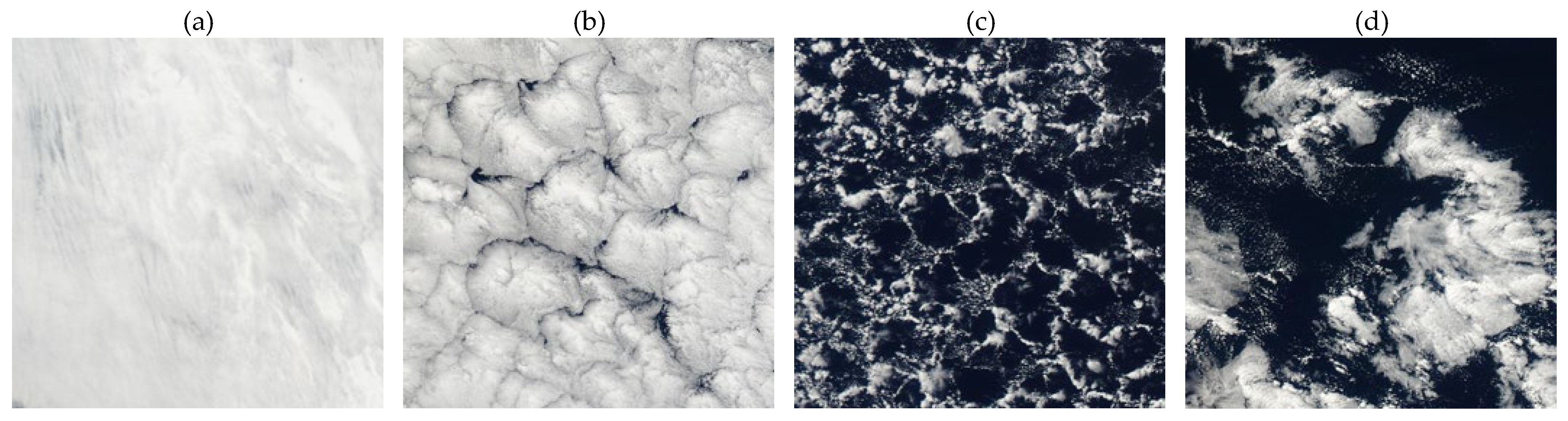
Figure 2.
A schematic of the VLM framework and training procedure used in this study. A similar framework is developed for marine Sc cloud types. Abbreviations: MCC: mesoscale cellular convection, CV: cross-validation, ViT: Vision Transformer. Symbols: : image embedding vector for the ith sample from the frozen image encoder; : text embedding vector for the sample ith from the frozen text encoder; , : learnable projection matrices for image and text embeddings, respectively; , : normalized projections of the image and text embeddings, respectively; : cosine similarity matrix, where each element represents the similarity between and ; P: precision; R: recall; F1: F1-score; A: accuracy. More details are provided in the text.
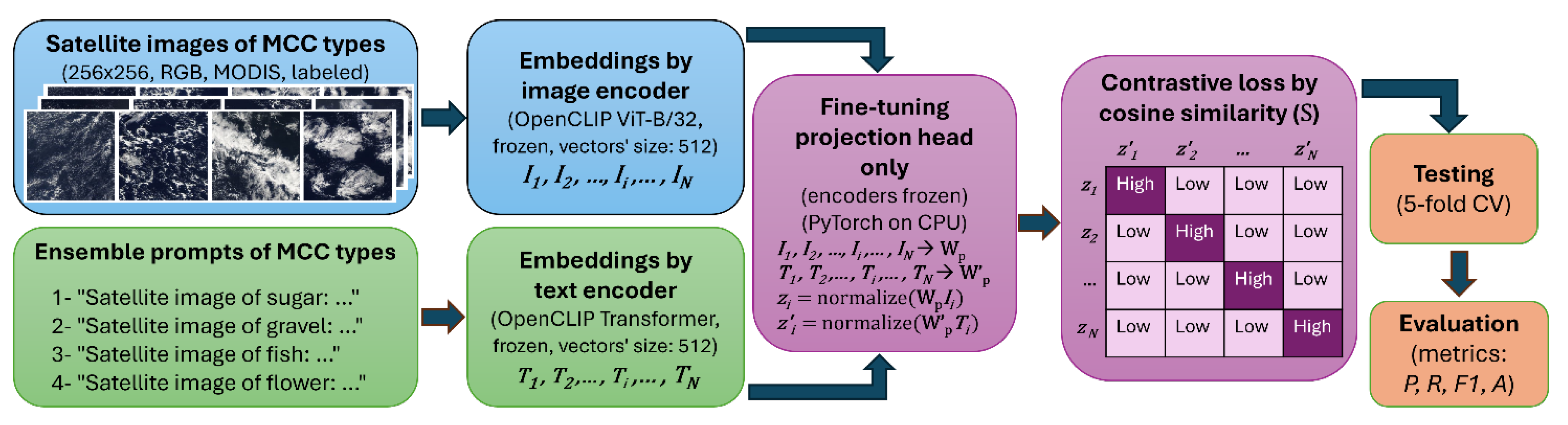
Figure 3.
Confusion matrices for image–only and prompt–image VLM configurations, showing the percentage of correctly and incorrectly classified samples for each SGFF MCC cloud category after 5-fold cross-validation. Note that values are normalized by the number of samples in each true class.
Figure 3.
Confusion matrices for image–only and prompt–image VLM configurations, showing the percentage of correctly and incorrectly classified samples for each SGFF MCC cloud category after 5-fold cross-validation. Note that values are normalized by the number of samples in each true class.
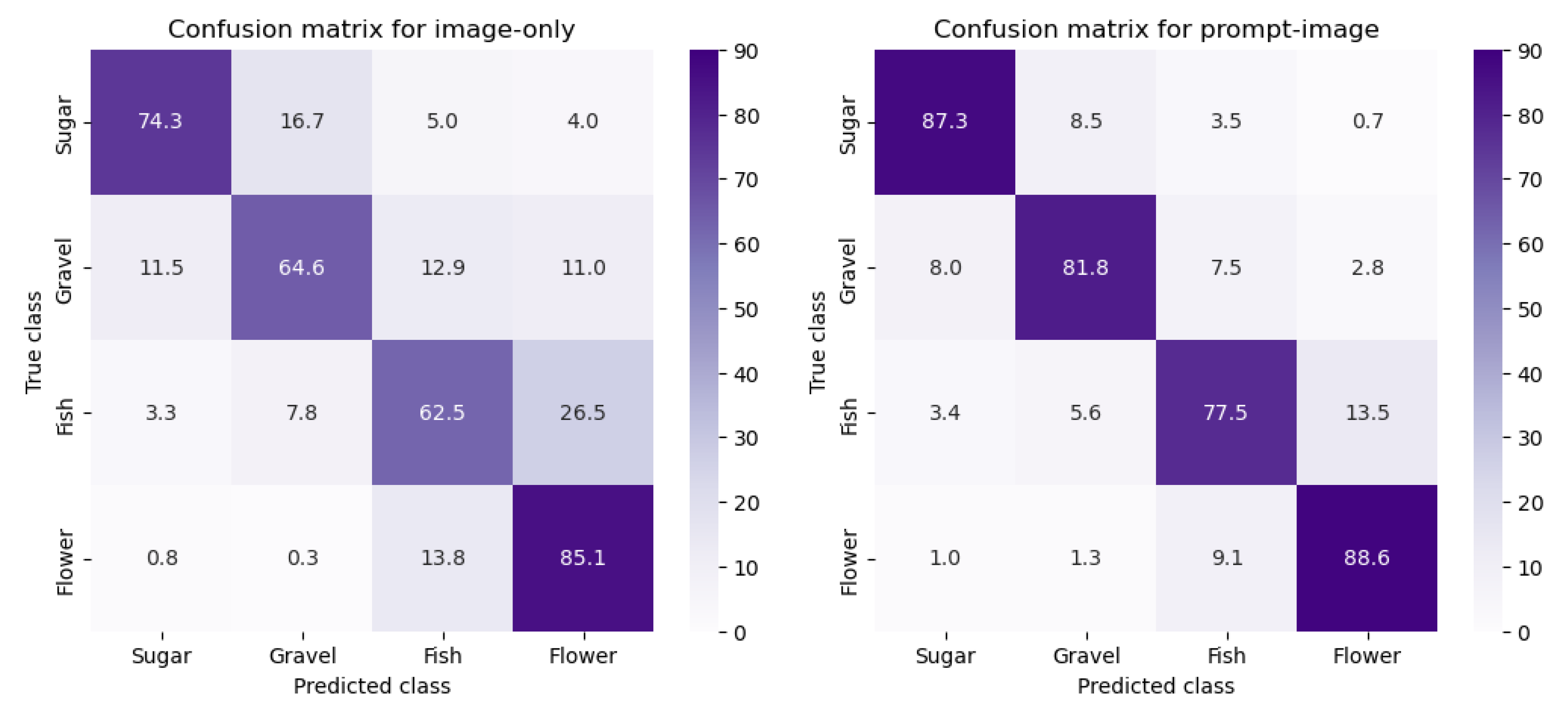
Figure 4.
Sensitivity of classification accuracy to training sample size for image-only (red) and prompt-image (blue) configurations. For each sample size, five random subsamples are drawn, the VLM is trained on each subsample, and k-fold cross-validation is performed to calculate accuracy (light markers and lines). The mean accuracy across the five subsamples is shown with darker markers and lines.
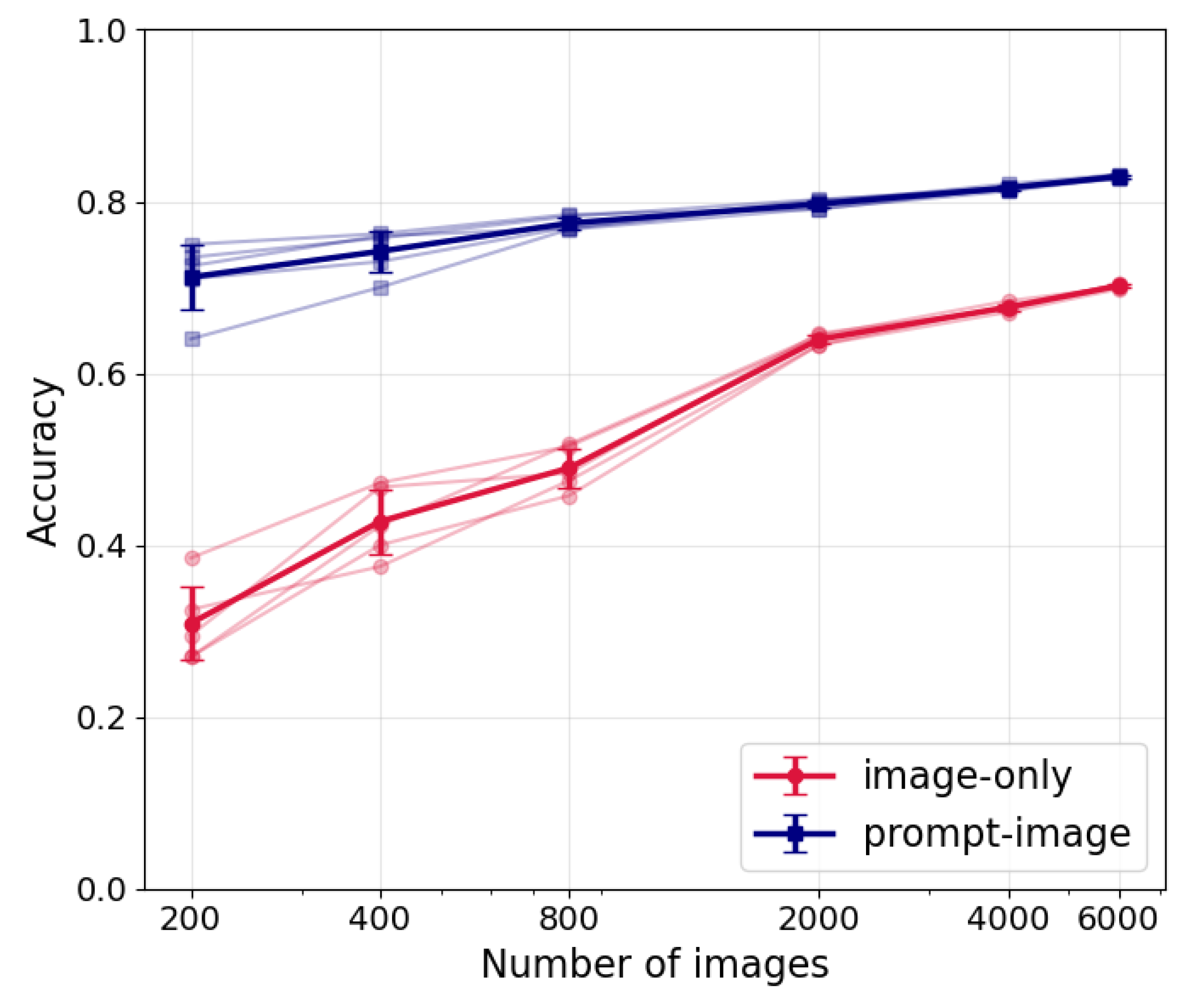

Table 1.
Evaluation metrics for image–only and prompt–image VLM configurations after 5-fold cross-validation. Precision, recall, and F1-score are reported for each SGFF MCC category, along with macro averages across all categories and overall accuracy.
Table 1.
Evaluation metrics for image–only and prompt–image VLM configurations after 5-fold cross-validation. Precision, recall, and F1-score are reported for each SGFF MCC category, along with macro averages across all categories and overall accuracy.
| Evaluation metrics for image-only | ||||
| Cloud type | Precision | Recall | F1-score | Accuracy |
| Sugar | 0.827 | 0.743 | 0.782 | --- |
| Gravel | 0.723 | 0.646 | 0.683 | --- |
| Fish | 0.664 | 0.625 | 0.644 | --- |
| Flower | 0.672 | 0.851 | 0.751 | --- |
| Total | 0.721 | 0.716 | 0.715 | 0.716 |
| Evaluation metrics for prompt-image | ||||
| Cloud type | Precision | Recall | F1-score | Accuracy |
| Sugar | 0.877 | 0.873 | 0.875 | --- |
| Gravel | 0.841 | 0.818 | 0.829 | --- |
| Fish | 0.794 | 0.775 | 0.784 | --- |
| Flower | 0.839 | 0.886 | 0.862 | --- |
| Total | 0.838 | 0.838 | 0.838 | 0.838 |
Table 2.
As in Table 1, but for marine Sc cloud categories.
Table 2.
As in Table 1, but for marine Sc cloud categories.
| Evaluation metrics for image-only | ||||
| Cloud type | Precision | Recall | F1-score | Accuracy |
| Open cells | 0.375 | 0.185 | 0.247 | --- |
| Closed cells | 0.351 | 0.523 | 0.420 | --- |
| Stratus | 0.449 | 0.477 | 0.463 | --- |
| Other cells | 0.516 | 0.492 | 0.504 | --- |
| Total | 0.423 | 0.419 | 0.408 | 0.419 |
| Evaluation metrics for prompt-image | ||||
| Cloud type | Precision | Recall | F1-score | Accuracy |
| Open cells | 0.809 | 0.846 | 0.827 | --- |
| Closed cells | 0.984 | 0.938 | 0.961 | --- |
| Stratus | 0.883 | 0.815 | 0.848 | --- |
| Other cells | 0.786 | 0.846 | 0.815 | --- |
| Total | 0.865 | 0.862 | 0.863 | 0.862 |
Disclaimer/Publisher’s Note: The statements, opinions and data contained in all publications are solely those of the individual author(s) and contributor(s) and not of MDPI and/or the editor(s). MDPI and/or the editor(s) disclaim responsibility for any injury to people or property resulting from any ideas, methods, instructions or products referred to in the content. |
© 2025 by the authors. Licensee MDPI, Basel, Switzerland. This article is an open access article distributed under the terms and conditions of the Creative Commons Attribution (CC BY) license (http://creativecommons.org/licenses/by/4.0/).
Copyright: This open access article is published under a Creative Commons CC BY 4.0 license, which permit the free download, distribution, and reuse, provided that the author and preprint are cited in any reuse.


