
Submitted:
28 August 2025
Posted:
28 August 2025
You are already at the latest version
Abstract
Recently, deep learning models such as convolutional neural network (CNN), convolutional autoencoder (CAE), CNN-based support vector machine (SVM), YOLO, fully convolutional network (FCN), fully convolutional data description (FCDD) and so on have been being applied to defect detections and anomaly detections of various kinds of industrial products, materials and systems. In those models, downsampled images including target features to be fitted to the resolution of each input layer are basically used for training and testing data. In this paper, intelligent anomaly diagnosis system for numerical control (NC) machine tools is considered, in which a simple microphone is positioned as the only sensor we use. Generally, mechanical sound and vibration generated from a machine tool itself or machining sound and vibration generated from a router bit, i.e., end mill cutter attached to the spindle head can be recorded and used for training NN models. Dataset used in this paper consists of operating sounds recorded from five different types of machines using a smartphone microphone. Since cost reduction is generally required in building systems, no special vibration or acceleration sensors are used. For experimental evaluation, nine kinds of mechanical sounds are collected from the five machine tools, and then training datasets consisting of sound blocks are prepared. Each sound block (SB) is time series data extracted from WAV (Waveform Audio File Format) files (.wav). For example, if a WAV file is recorded with a sampling rate 44100 [Hz] and an extracted time for forming a SB is set to 0.005 [s], then the data length of the sound block approximately becomes 220. The extracted SBs from a WAV file are employed for training three types of NN models for classification. As for the NN models for comparison, conventional shallow NN, RNN and 1D CNN are designed and trained using the nine kinds of mechanical sounds. Classification results of test SBs by the three models are shown. Then, an autoencoder is designed and considered for identifier by training it using only SBs of a machine tool. One of the technical needs in dealing with time series data such as SB data by NN is how to clearly visualize and understand anomalous regions in concurrent with identification. In this paper, finally, we propose the SB data-based FCDD model to meet this need. The superiority of the FCDD model is verified in terms of anomaly detection accuracy and concurrent visualization of understanding.
Keywords:
1D CNN
; Autoencoder
; Sound block (SB)
; SB data-based FCDD
; Identification
; Anomaly detection
; Visualization of understanding
1. Introduction
In order to solve the issues related to product quality control faced by the manufacturing industry, the authors is developing an application that can easily and effectively design and train a machine learning model that has the same or more ability to identify defective products as skilled inspectors. Figure 1 and Figure 2 show the main and sub dialogues developed on MATLAB. By using the proposed application, the authors are supporting engineers to built their desired machine learning models for defect detection of industrial products and materials included in images and movies. Available models are convolutional neural network (CNN), convolutional autoencoder (CAE), support vector machine (SVM), you look only once (YOLO) [1,2], U-Net, segmenting objects by locations (SOLO) [3,4], mask region-based CNN (Mask R-CNN) [5], fully convolutional data description (FCDD) and so on [6]. In fact, in manufacturing industries, there is a strong need for flexible anomaly detection systems that allow workers to easily cope with all the processes from setting up the environment to operating the system, so that we are evaluating and improving the application through trial use, and expanding functionality based on feedbacks from users.
Up to now, many relevant researches of anomaly detection system based on sound data have been proposed. Harada et al. proposed a baseline system for first-shot-compliant unsupervised anomaly detection for machine condition monitoring, in which a simple autoencoder-based implementation combined with a selective Mahalanobis metric is implemented as a baseline system. The performance is evaluated to set the target benchmark for the forthcoming Detection and Classification of Acoustic Scenes and Events (DCASE2023T2) [7]. Zhou et al. proposed an incremental learning-based anomaly sound detection model that enhances the model’s capacity to learn from continuous data streams, reduces knowledge forgetting, and improves the stability of the model in anomaly sound detection task. Experiments using Task 2 data from the DCASE2020 challenge shows that the proposed method effectively improves the average AUC and average pAUC by 7% to 10% when compared to the fine-tuning strategy [8]. Also, Dong et al. proposed a self-encoder model combining residual CNN and long and short-term memory (LSTM) network is used to extract features in both spatial and temporal dimensions, respectively, to make full use of the information of the audio signal [9]. In addition, Sekhar et al. proposed a texture analysis-based transfer learning CNN models so that they can be applied to a three classes (high/medium/low tool wear) classification task of tool wear based on the noise generated during mild steel machining. Machining acoustics were converted to spectrogram images so that they can be given to the input layer of each CNN, in which four pre-trained models as SqueezeNet, ResNet50, InceptionV3, GoogLeNet were used for backbone.
However, there seems to be almost no discussion about the optimal way to design sound data for training machine learning models. Also, it seems that concurrent visualization of understanding in time domain is not well realized when NN models are applied to anomaly detection of time series data such as acoustics data. In this paper, the authors have considered neural network systems that can be easily applied to classification, anomaly detection and prediction of NC machine tools as shown in Figure 3. In addition to images and videos used for training, in order that time series data such as mechanical sounds and vibrations can be used as multidimensional vector data, design functions for shallow NN, recurrent NN, 1D CNN, and AE are implemented in the application shown in Figure 2. For training machine learning models, many sound block (SB) data extracted with a designated sampling time are generated from nine categories of mechanical sounds collected from multiple machine tools. We report on the evaluation of the classification performance of each model on test data while changing the extraction time, which determines the length of the sound block, and the number of sound blocks used for training.
Finally, SB data-based FCDD is proposed for multi-dimensional vector data to realize anomaly detection of time-series data and its concurrent visualization of understanding, in which for example, time series sound data are converted to 1 line gray-scale images followed by BMP images for training FCDD. The effectiveness of the proposed model is evaluated by experiments.
2. Machining Tool Operating Sound and Sound Blocks
In the experiment, multiple machine tools installed at the university’s machine design and manufacturing center were operated, and operating sounds from nine categories were collected for 10 seconds at a sampling rate of 44100 [Hz] using a smartphone and saved in WAV files. Sound blocks extracted from WAV files are used for training neural network models. Figure 4 shows an example of extraction of time series sound block data from a WAV file which is recorded from a general purpose milling machine. In this experiment, sound block data are sampled with 0.005 [s], so that the length of a SB data file is 44100×0.005≒220.
According to the length, the number of input layer’s neurons is designed as 220. Also, in this case, the number of sound blocks extracted from a WAV file becomes 2000, whose 80%, 10%, and 10% are assigned for training, validation, and test, respectively
3. Training and Evaluation of a Classical Shallow Neural Network
3.1. Neural Networks for Classification
Table 1 shows the numbers of sound blocks prepared for training, evaluation, and test of nine categories. Also, Figure 5 and Figure 6 shows four layered normal neural networks and recurrent neural networks, respectively. The numbers of units in the first and second hidden layers 100 and 50, respectively. Moreover, Figure 7 shows the structure of 1D CNN consisting of 11 layers, in which the number N of labels from the output layer is 9 according to the classification task of 9 categories.
After trained by the adaptive moment estimation (ADAM) [10] and cross entropy loss, these neural network models were compared and evaluated through a classification task of test sound block data. As a result, mean values of classification accuracies are 87.6%, 88.4%, and 99.5%, respectively. Although there was no significant difference in classification performance between NN and RNN, higher classification performance was obtained with 1D CNN. As for training time, also, although approximately tens of thousands of epochs were needed for conversion of NN and RNN, 1D CNN could be training in shorter training time. Actually, the numbers of training weight parameters of NN, RNN, and 1D CNN were 27,609, 52,609, 11,273, respectively. Table 2 shows each layer’s output activation and the numbers of parameters. Note that the meanings of T and C are time series data and the number of channels, respectively. It is expected from the above results that, in the future, anomaly detection using 1D CNN will be possible by accumulating both of normal and anomaly machining sounds.
3.2. Autoencoder for Anomaly Detection
When the objective is to detect abnormalities in machine tools, etc., it seems effective to apply an autoencoder model that can be trained using only normal machining sounds. In this evaluation experiment, an autoencoder is designed as shown in Figure 8. A structural feature of the autoencoder is that the input and output layers have the same number N of units. The loss function is given by Eq. (1) which is composed of the mean suared error (MSE) loss, L2 regularization term of weights, and sparse regularization term based on Kullback Leibler Divergence (KLD) [11]. The autoencoder is trained so that sound blocks at the input layer can be equivalently generated from the output layer. The autoencoder is trained such that every sound block in the training data given to the input layer can be neuron-level-equally reconstructed as at the output layer.
where N is the length of a sound block, which is the number of units both in input and output layers. H and M are the numbers of units in the hidden layer and that of all the sound blocks in training data. are the weights between the input layer and hidden layer, are those between the hidden layer and output layer. Also, and are the coefficients to weight the degrees of penalties of L2 regularization and sparse regularization, respectively. Note that in the third term is the mean value of activation generated by the sigmoid function h at the ith unit in the hidden layer, which is given by
where is the ith row data in the weight matrix , is the jth training data. Note that in Eq. (1) is the desired value of , to which 0.05 is set. As can be seen, the loss function to train the autoencoder is composed of the first term about MSE, the second term about L2 regularization, and third term about sparse regularization based on KLD.
In training the autoencoder, the reconstruction loss included in Eq. (1) according to an input of sound block is given by
A threshold value is defined as the maximum value of obtained during the training. After training, if obtained from a SB for test is under the threshold value, then the SB is predicted as the same machine with the autoencoder, otherwise a different machine. This means that if the autoencoder is trained using the SB data extracted from one machine tool, a test SB data can be predicted as the same machine or not.
In experiments, SB data of a band saw shown in Table 1 is used for training the autoencoder. At the first step, the extracted time of a sound block is set to 0.005 [s], i.e., data length N is set to 220 (), however, a successful classification result could not be obtained. Accordingly, the extracted time is gradually increased to 0.05, i.e., N=2205, so that each 300 test SB data except the band saw could be well identified as different from those of the band saw as shown in Table 3. Note that the number of neurons H in the hidden layers is 1000, consequently, that of all the weight parameters is 4,413,205. It is expected from the results that detection of anomaly mechanical sound will be possible by training the autoencoder based on the sound in normal situation.
4. SB Data-Based FCDD Model for Anomaly Detection and Visualization of Time Series Data
It has been confirmed from the experiments up to the previous sections that 1D CNN and autoencoder are effective for classification and identification of SB data, respectively. As can be expected, 1D CNN is also applied to anomaly detection tasks by redesigning the output layer for binary classification, i.e., normal and anomaly.
4.1. The Proposed FCDD for Time Series Data such as SB Data
At this stage, one of serious problems in dealing with the time series data such as SB data is how clearly and concurrently anomaly areas should be visualized and understood. In this paper, to cope with need, a SB data-based FCDD model is further proposed as shown in Figure 9 to perform anomaly detection and its concurrent visualization without secondly using Grad-CAM [12] or Occlusion Sensitivity [13]. The proposed method allows us to construct an FCDD-based anomaly detection system for time series data such as SB data.
Objective function of FCDD [14] is briefly introduced. In Liznerski’s paper, an FCN model employed in the former part performs , by which a feature map downsized into is generated from an input image X. A heat map of defective regions can be produced based on the feature map. The pseudo-Huber loss [15] in terms of an output matrix from the FCN part, i.e., a feature map is given by
where the calculation is done with element-wise operation, i.e., pixel-wisely to be able to form a heat map. The object function in training an FCDD model is given by
The first term has a valid value in case that the label of a training image is negative, i.e., , where L1 norm is divided by the total pixels of a feature map. The value can be considered as the average per one pixel. Therefore, when normal images are given to the network in training, the weights are adjusted so that each pixel forming a heat map can approach to 0.
On the other hand, the second term becomes effective when the label of a training image is anomaly (), and has a value close to 0 with the increase of the average loss per one pixel, so that the value of log function also approaches to 0 with the lapse of training time. It is confirmed from the above discussion that Eq. (5) using Eq. (4) enables both to minimize the sum of the averages of of non-defective images and to maximize those of defective images. The main dialogue shown in Figure 1 enables to user-friendly train, test and built FCDD models.
4.2. How to Generate Image Data from SB data
In this subsection, it is explained that how to generate input images for FCDD from SB data in time-series domain. As shown in Figure 9, X has the same resolution with the input layer of FCDD. As already explained, A SB data is directly extracted from a WAV file with a designated extraction time [s]. For example, if the sampling frequency of a WAV file is f [Hz] , then the length N of a SB data becomes . 1 line SB data is transformed to 1 line gray-scale BMP image as shown in Figure 10 through normalization by
where and are the maximum and minimum values of elements in s, respectively. Then, an expanded bitmap image to be given to the input layer of FCDD can be constructed as
4.3. Experiment of Identification of Machine Tools’ Sound Data and Its Concurrent Visualization Using an FCDD Model
In this subsection, an identification experiment is conducted using the nine kinds of SB data as shown in Table 4, in which it is assumed that the sound of Band-Saw is normal and other eight kinds of sounds are anomaly, so that 30 normal SBs and 30×8=240 anomaly SBs are used for training the FCDD model. After 200 epocks of training, all the training data were scored as shown in Figure 11. In order to use the trained FCDD as an anomaly detector, a threshold value for criteria has to be set. In this case, a threshold value 1 of anomaly score can be easily determined from the distribution in Figure 11.
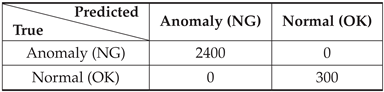
After setting 1 to the threshold value, generalization ability was checked using test SB data. 300 normal SBs and 300×8=2400 anomaly SBs were used for testing, so that all the images could be accurately classified to normal (Band-Saw) or anomaly (Except for Band-Saw) as shown in Table 5. Figure 12 shows the histogram of the test SB data’s mean anomaly scores predicted by the FCDD model. Figure 13 also shows examples of predicted maps generated by the FCDD, in which it is observed that anomaly regions within the time series data are validly visualized.
5. Conclusions
The authors have been developing a design, training and building application with a user-friendly operation interface for CNN, CAE, SVM, YOLOX, SOLOv2, FCDD, and so on, which can be used for the defect detection of various kinds of industrial products even without deep skills and knowledge concerning information technology. In those models, images are basically used for training data. In this paper, an intelligent anomaly diagnosis system for NC machine tools is considered, i.e., what structures of neural networks should be applied to this task. Mechanical sound and vibration generated from machine tools themselves or machining sound and vibration generated from router bits, i.e., end mill cutters are recorded as wave files and used for training data. Extracted SB data from wave files are employed for training NN models. It is confirmed from experiments that a 1D CNN and an autoencoder are effective for a sound classification task and a sound identification one, respectively. In this paper, a SB data-based FCDD model is further proposed for anomaly sound detection of removal machining by NC machine tools and its concurrent visualization, in which time series data such as SB data can be directly applied to training and testing without converting them to other domain such as frequency. The effectiveness of the proposed method is shown through experiments.
Author Contributions
Conceptualization, F.N. and K.W.; Methodology, F.N. and T.M.; Software, F.N. and T.M.; Validation, F.N. and T.M.; Formal analysis, F.N. and T.M.; Investigation, F.N. and T.M.; Resources, F.N. and T.M.; Data curation, F.N.; Writing—original draft preparation, F.N. and M.K.H.; Writing—review and editing, F.N., M.K.H. and K.W.; Visualization, F.N.; Supervision, F.N. All authors have read and agreed to the published version of the manuscript.
Funding
This research received the external funding as JSPS KAKENHI Grant Number JP25K07532.
Data Availability Statement
Data are contained within the article.
Acknowledgments
This work was supported by JSPS KAKENHI Grant Number JP25K07532.
Conflicts of Interest
The authors declare no conflicts of interest.
Abbreviations
The following abbreviations are used in this manuscript:
| ADAM | Adaptive Moment Estimation Optimizer |
| CAE | Convolutional AutoEncoder |
| CNN | Convolutional Neural Network |
| FCDD | Fully Convolutional Data Description |
| FCN | Fully Convolution Network |
| Grad-CAM | Gradient-Weighted Class Activation Mapping |
| HSC | Hyper Sphere Classifier |
| SGDM | Stochastic Gradient Decent Momentum Optimizer |
| SVM | Support Vector Machine |
| VAE | Variational AutoEncoder |
References
- Z. Ge, S. Liu, F. Wang, Z. Li, and J. Sun, “YOLOX: Exceeding YOLO Series in 2021," arXiv, August 5, 2021. http://arxiv.org/abs/2107.08430 (accessed on 25 August 2025). [CrossRef]
- https://jp.mathworks.com/help/vision/ug/getting-started-with-yolox-object-detection.html (accessed on 25 August 2025).
- X. Wang, T. Kong, C. Shen, Y. Jiang, and L. Li, “SOLO: Segmenting Objects by Locations," In Proc. of European Conference of Computer Vision (ECCV2020), pp. 649–665, 2020. https://arxiv.org/abs/1912.04488 (accessed on 25 August 2025). [CrossRef]
- X. Wang, R. Zhang, T. Kong, L. Li, and C. Shen, “SOLOv2: Dynamic and Fast Instance Segmentation," ArXiv, October 23, 2020. [CrossRef]
- K. He, G. Gkioxari, P. Doll?r, and R. Girshick, “Mask R-CNN," Preprint, submitted January 24, 2018. https://arxiv.org/abs/1703.06870 (accessed on 25 August 2025). [CrossRef]
- F. Nagata, K. Nakashima, K. Miki, K. Arima, T. Shimizu, K. Watanabe, M.K. Habib, “Design and Evaluation Support System for Convolutional Neural Network, Support Vector Machine and Convolutional Autoencoder," Measurements and Instrumentation for Machine Vision, pp. 66–82, CRC Press, Taylor & Francis Group, July, 2024.
- N. Harada, D. Niizumi, Y. Ohishi, D. Takeuchi and M. Yasuda, “First-Shot Anomaly Sound Detection for Machine Condition Monitoring: A Domain Generalization Baseline," 2023 31st European Signal Processing Conference (EUSIPCO), Helsinki, Finland, 2023, pp. 191–195.
- H. Zhou, K. Wang, J. Yao, W. Yang and Y. Chai, “Anomaly Sound Detection of Industrial Equipment Based on Incremental Learning," 2023 CAA Symposium on Fault Detection, Supervision and Safety for Technical Processes (SAFEPROCESS), Yibin, China, pp. 1–6, 2023.
- W. Dong, F. Guo and T. Cheng, “Machine Anomalous Sound Detection Based on a Multi-dimensional Feature Extraction Self-encoder Model," 2024 5th International Conference on Computer Engineering and Application (ICCEA), Hangzhou, China, pp. 1165–1169, 2024.
- D. Kingma, J. Ba, “Adam: A Method for Stochastic Optimization." Procs. of the 3rd International Conference on Learning Representations (ICLR 2015), 15 pages, 2015.https://arxiv.org/pdf/1412.6980.pdf (accessed on 25 August 2025).
- https://jp.mathworks.com/help/deeplearning/ref/trainautoencoder.html (accessed on 25 August 2025).
- R.R. Selvaraju, M. Cogswell, A. Das, R. Vedantam, D. Parikh, D. Batra, “Grad-CAM: Visual Explanations from Deep Networks via Gradient-based Localization," Procs. of IEEE International Conference on Computer Vision (ICCV), pp. 618–626, 2017. [CrossRef]
- M.D. Zeiler, R. Fergus, “Visualizing and Understanding Convolutional Networks,” Computer Vision – ECCV 2014: 13th European Conference, Proceedings, Part III (Lecture Notes in Computer Science, 8691), pp. 818–833, Springer, 2014.
- P. Liznerski, L. Ruff, R.A. Vandermeulen, B.J. Franks, M. Kloft, K.R. Muller, “Explainable Deep One-Class Classification,” Procs. of International Conference on Learning Representations 2021, pp. 1–25, 2021. [CrossRef]
- P.J. Huber, “Robust Estimation of a Location Parameter," The Annals of Mathematical Statistics, Vol. 35, No. 1, pp. 73–101, 1964.
Figure 1.
Main dialogue developed on MATLAB system to user-friendly design CNN, SVM, CAE, FCDD, and so on.
Figure 1.
Main dialogue developed on MATLAB system to user-friendly design CNN, SVM, CAE, FCDD, and so on.
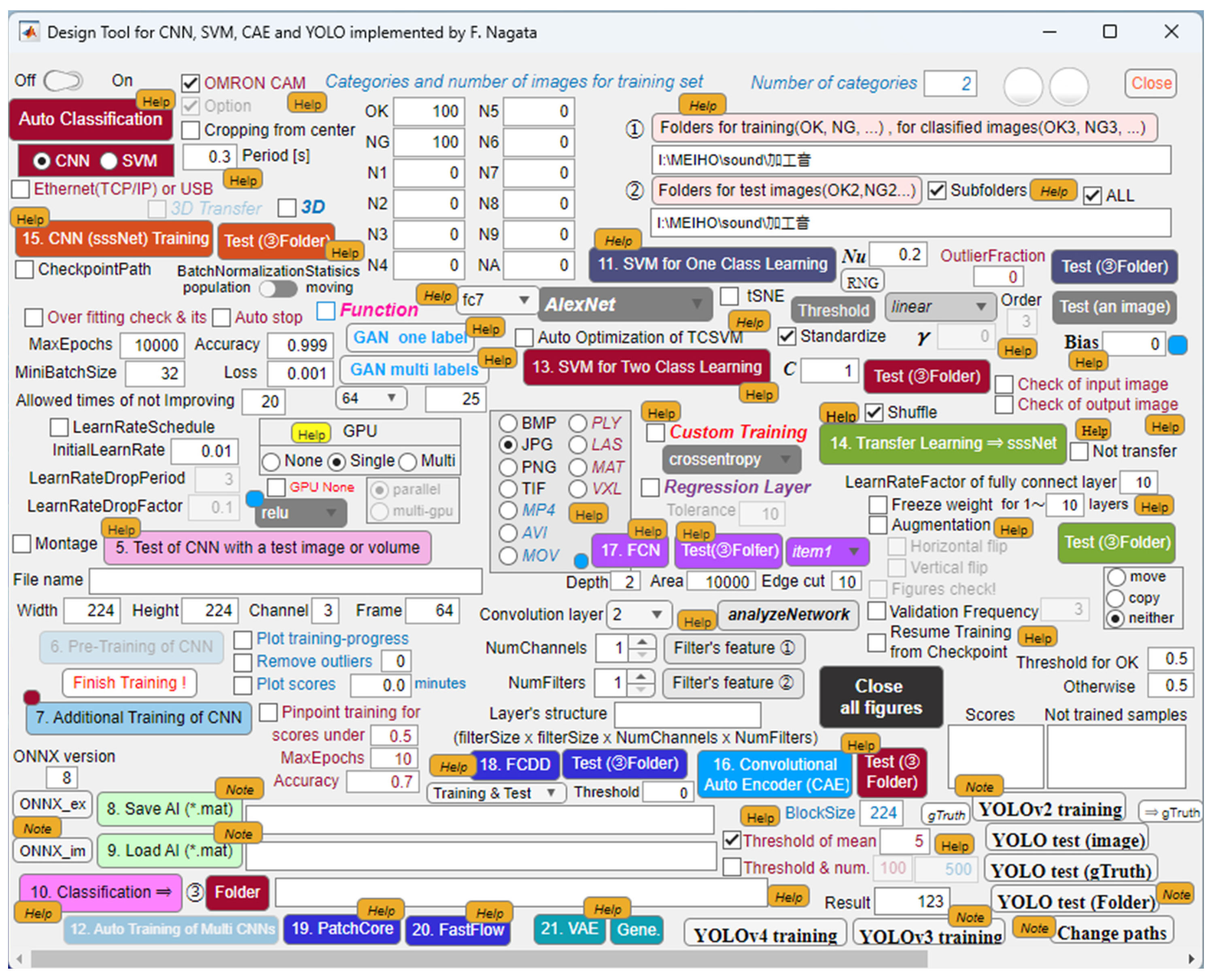
Figure 2.
Another dialogue to user-friendly design Shallow NN, RNN, VAE, 1D CNN, and so on.
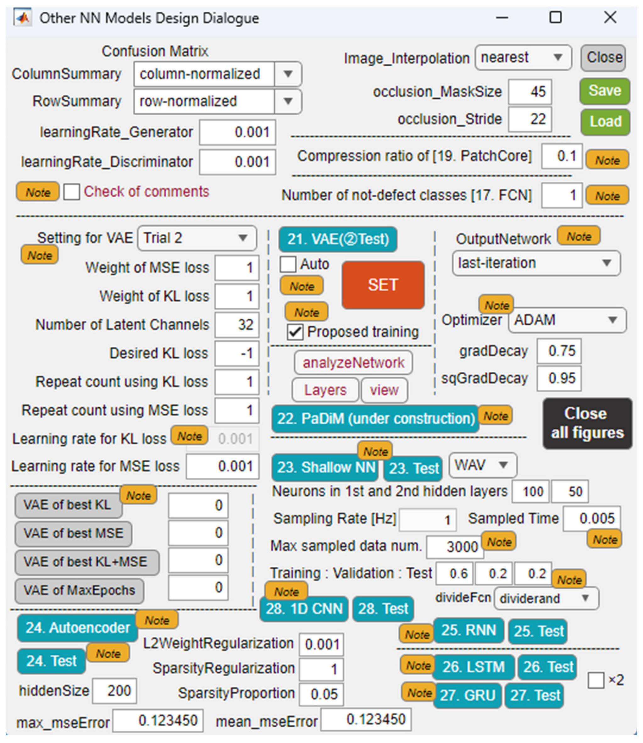
Figure 3.
Machining scene of a large wood material using a long ball-end mill for a long time (SOLIC Co. Ltd.).
Figure 3.
Machining scene of a large wood material using a long ball-end mill for a long time (SOLIC Co. Ltd.).
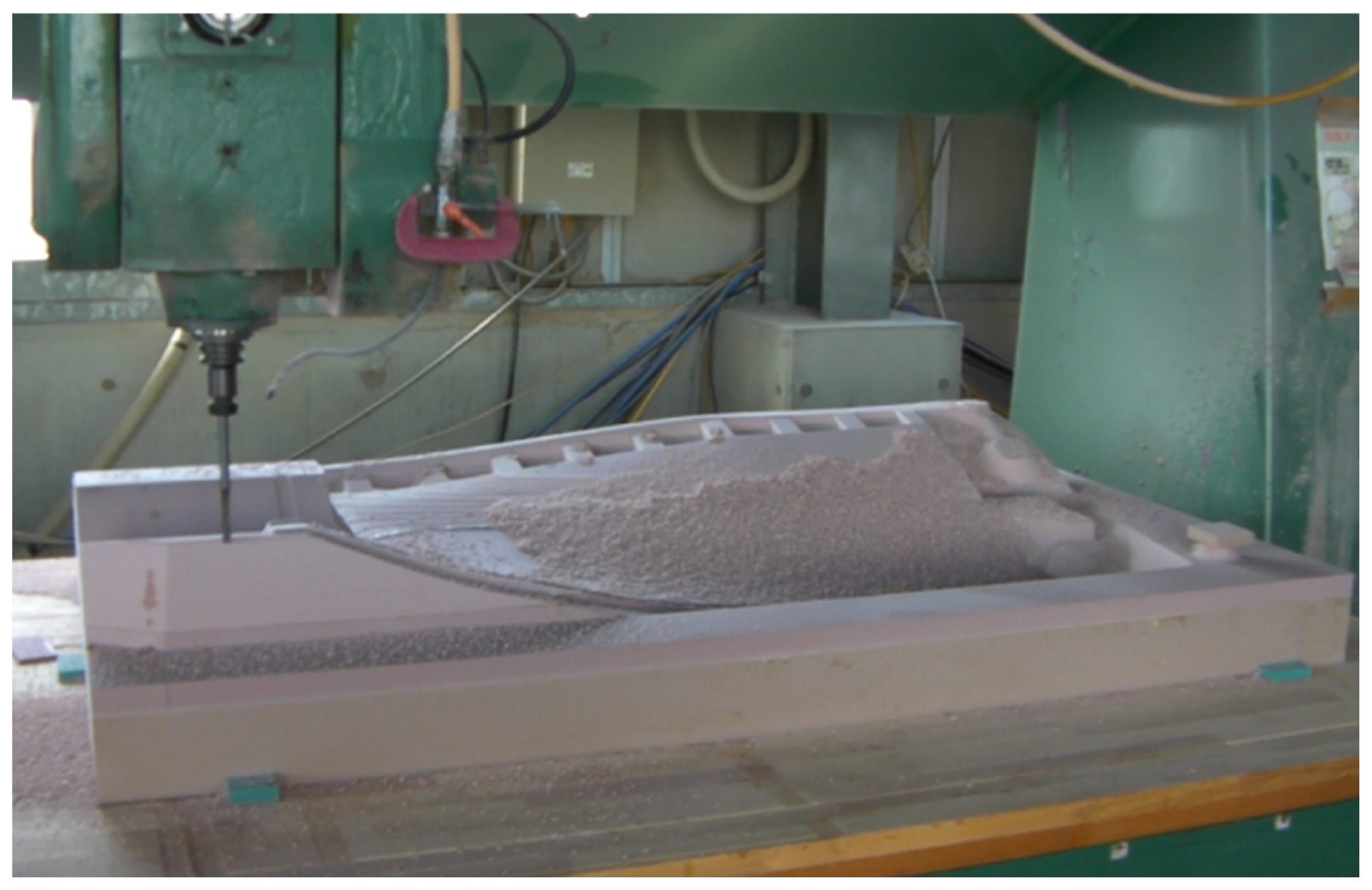
Figure 4.
Sound blocks extracted from a WAV file (.wav), which are used for training, evaluation, and test of NN models.
Figure 4.
Sound blocks extracted from a WAV file (.wav), which are used for training, evaluation, and test of NN models.
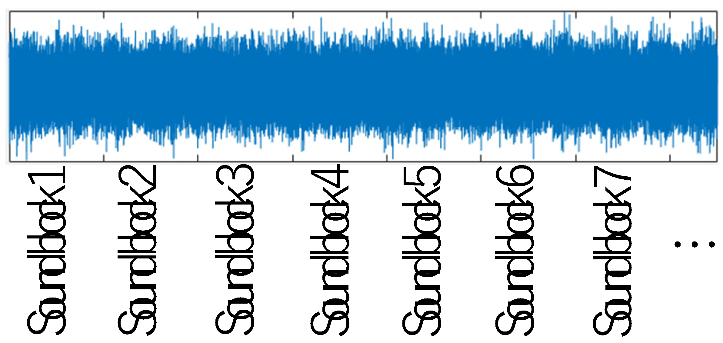
Figure 5.
Neural network whose input and output data are a sound block and stochastic variable given by Softmax function, respectively.
Figure 5.
Neural network whose input and output data are a sound block and stochastic variable given by Softmax function, respectively.
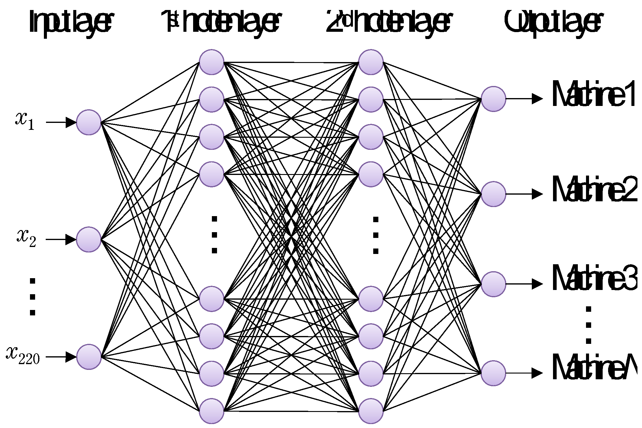
Figure 6.
Recurrent type neural network whose input and output are the same with those in Figure 5.
Figure 6.
Recurrent type neural network whose input and output are the same with those in Figure 5.
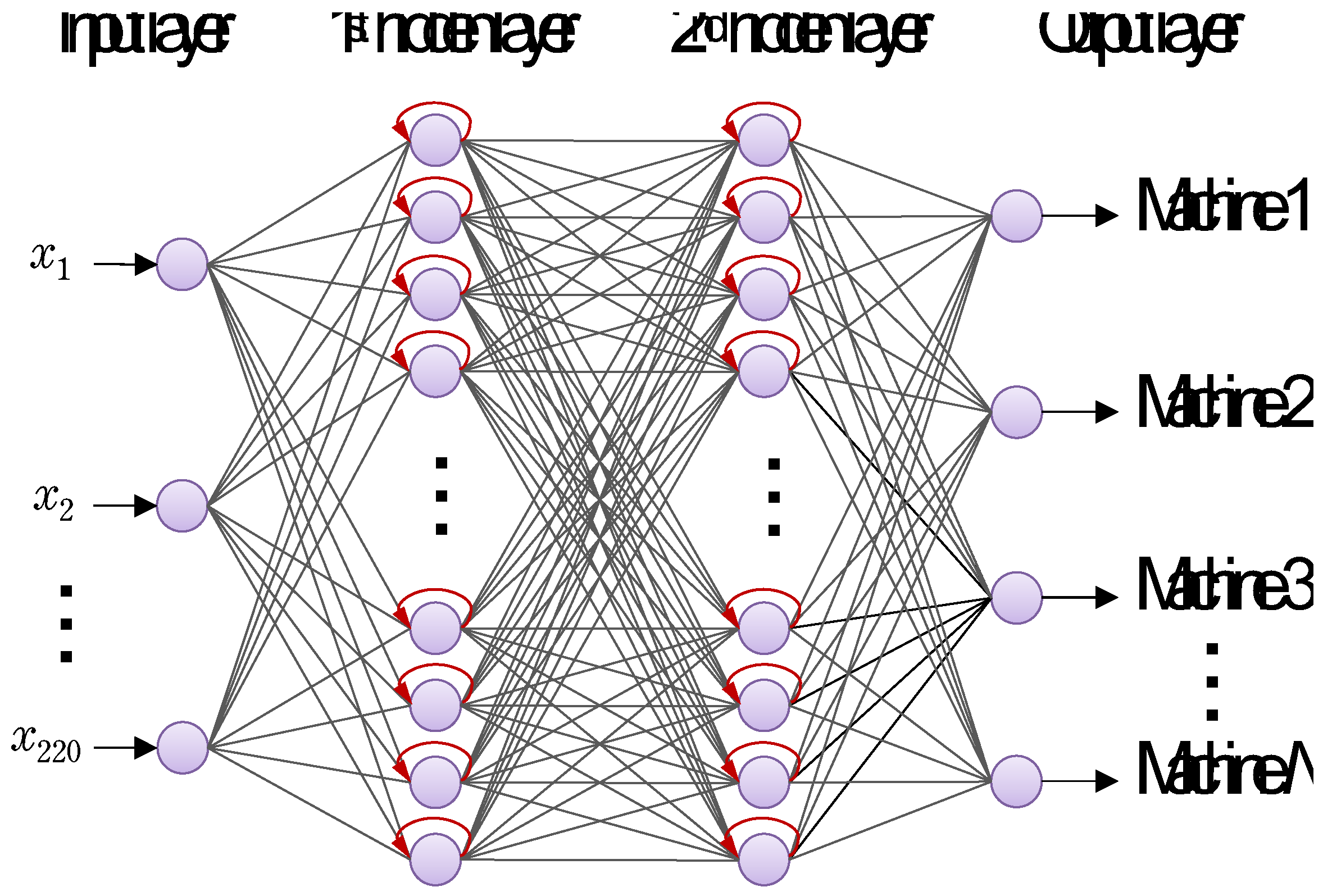
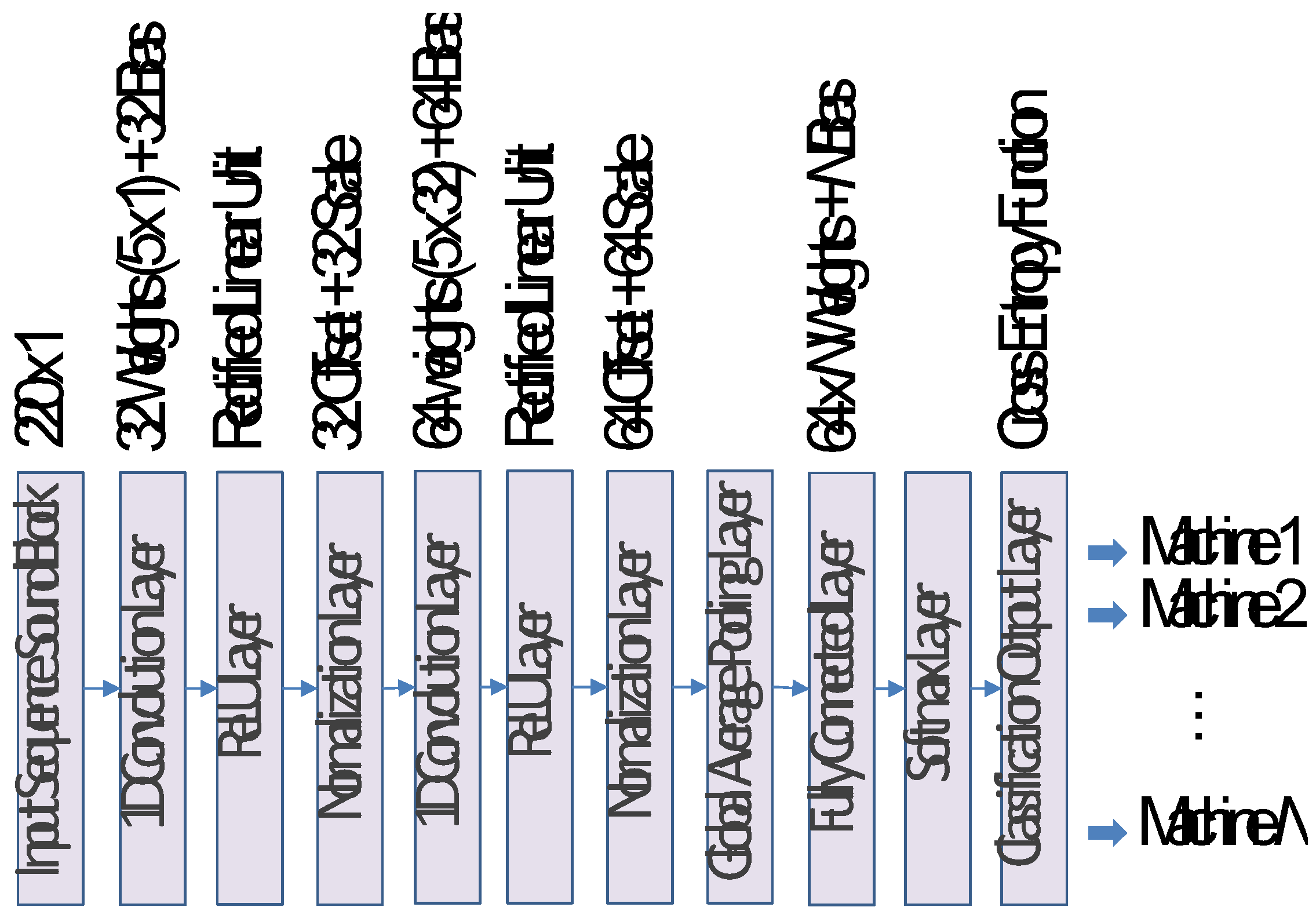
Figure 8.
Autoencoder with N=2205, whose input and output are a sound block and its reconstructed vector , respectively.
Figure 8.
Autoencoder with N=2205, whose input and output are a sound block and its reconstructed vector , respectively.
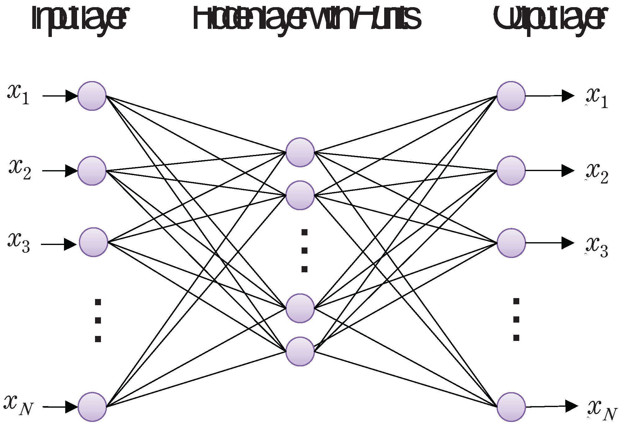
Figure 9.
Structure of our proposed SB data-based FCDD model for anomaly detection and its concurrent visualization.
Figure 9.
Structure of our proposed SB data-based FCDD model for anomaly detection and its concurrent visualization.
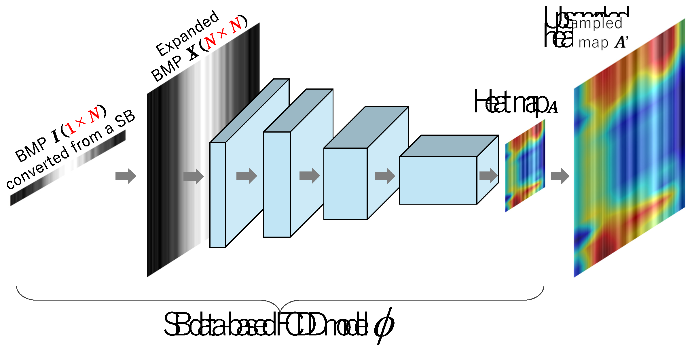
Figure 10.
BMP files generated from SB data for training an FCDD model.
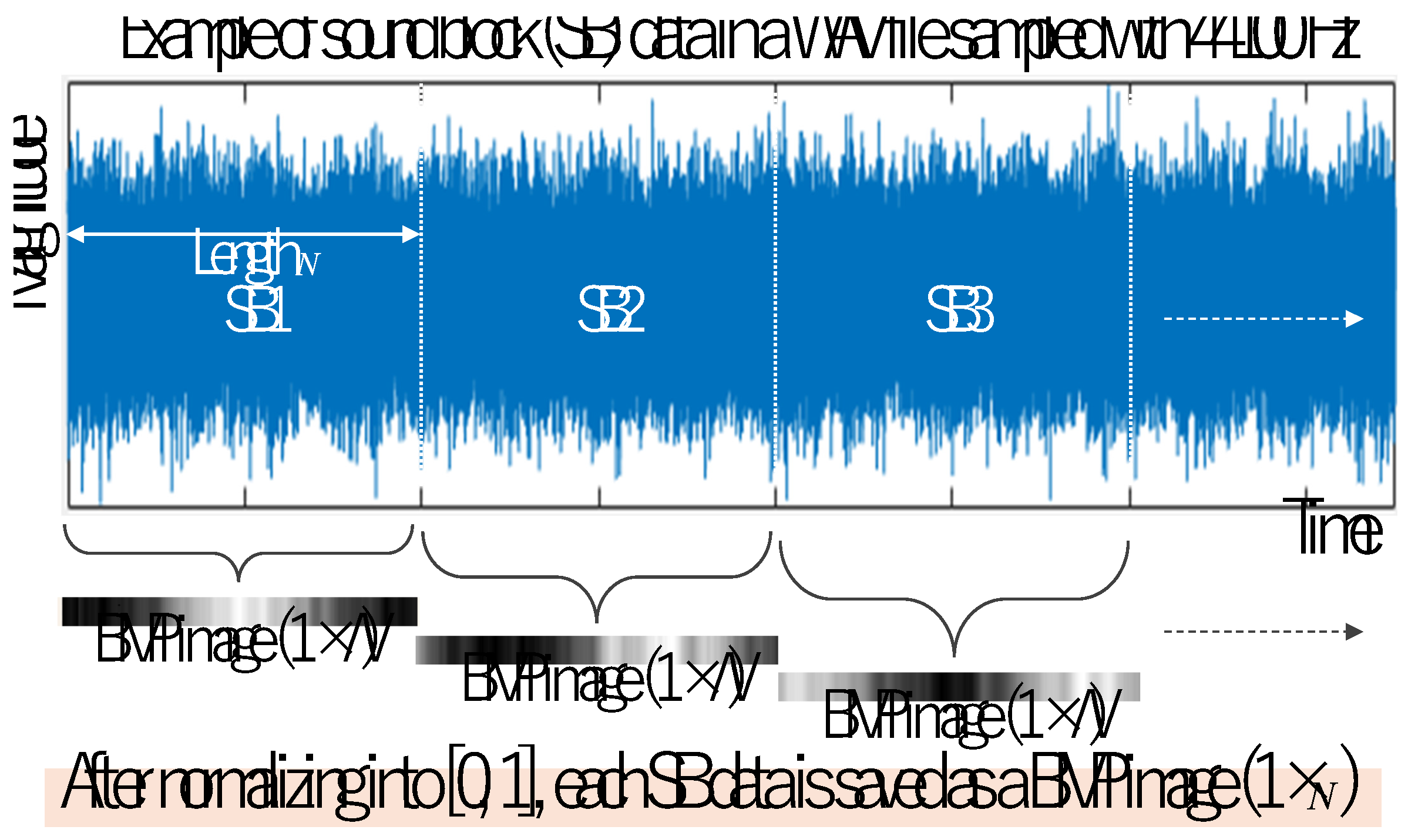
Figure 11.
Scores of training images evaluated by the trained FCDD model.
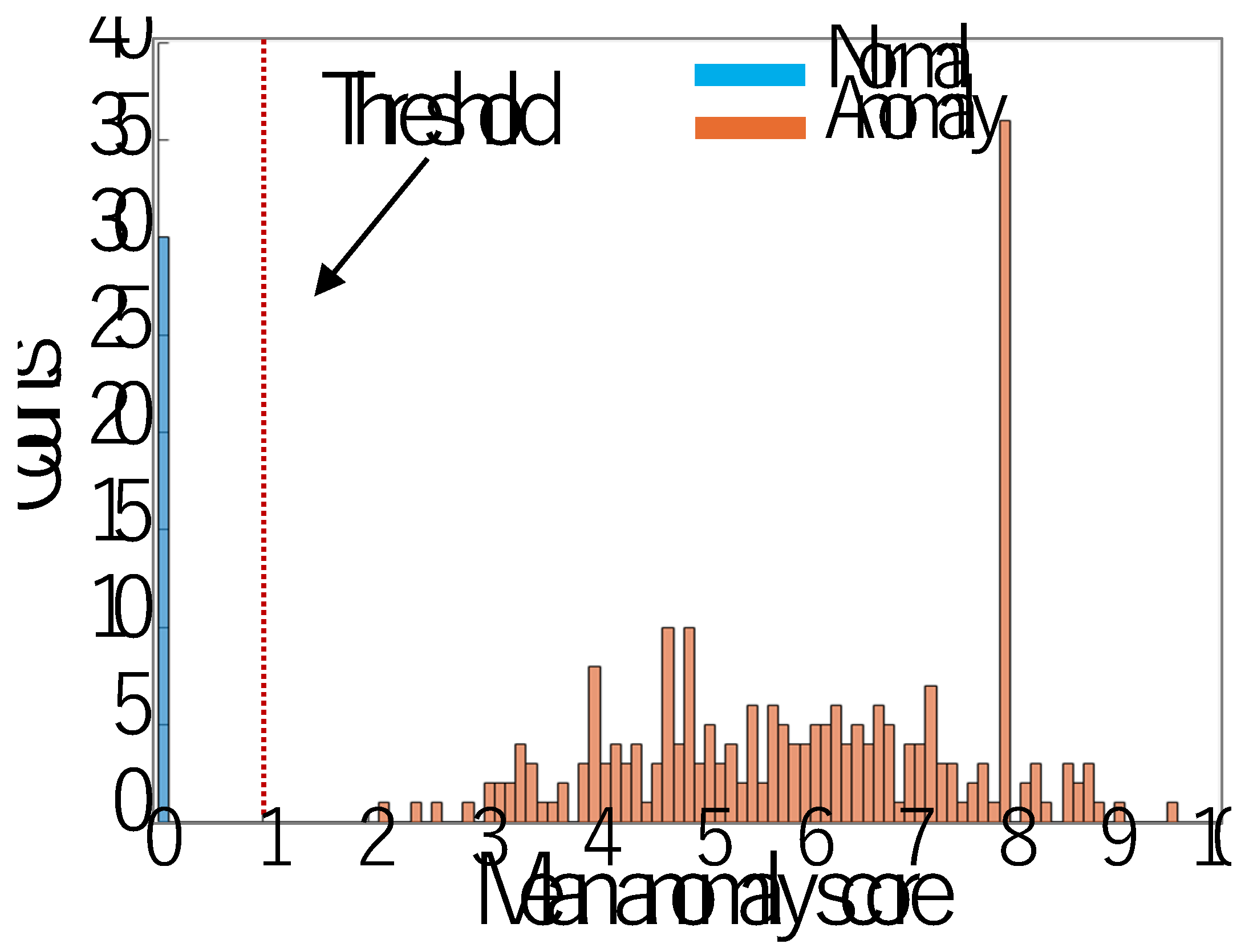
Figure 12.
Anomaly detection experiment using an FCDD Model, in which it is assumed that the sound of Band-Saw is normal and other sounds are anomaly.
Figure 12.
Anomaly detection experiment using an FCDD Model, in which it is assumed that the sound of Band-Saw is normal and other sounds are anomaly.
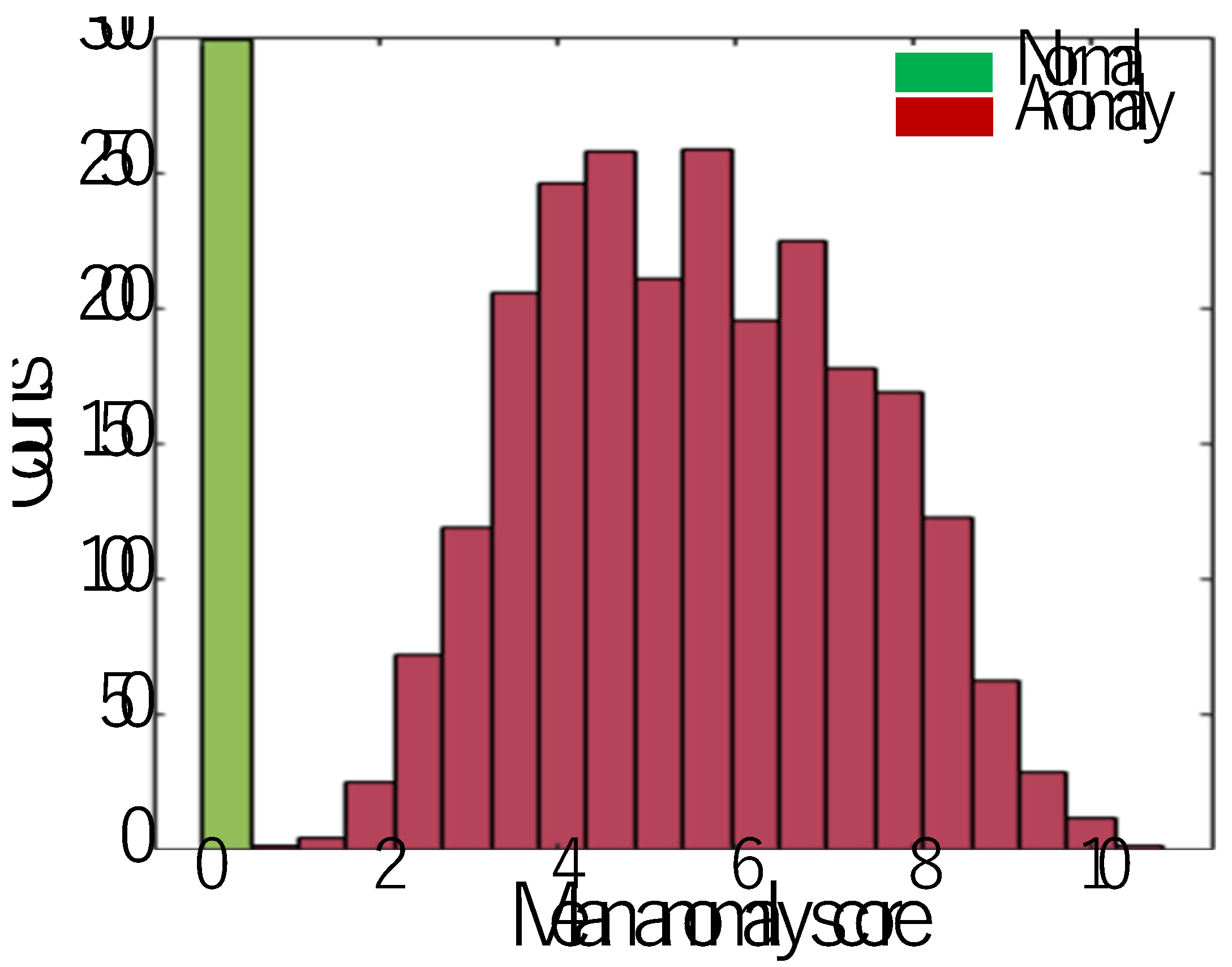
Figure 13.
Examples of visualization results of normal and anomaly sound areas generated by using the trained FCDD.
Figure 13.
Examples of visualization results of normal and anomaly sound areas generated by using the trained FCDD.
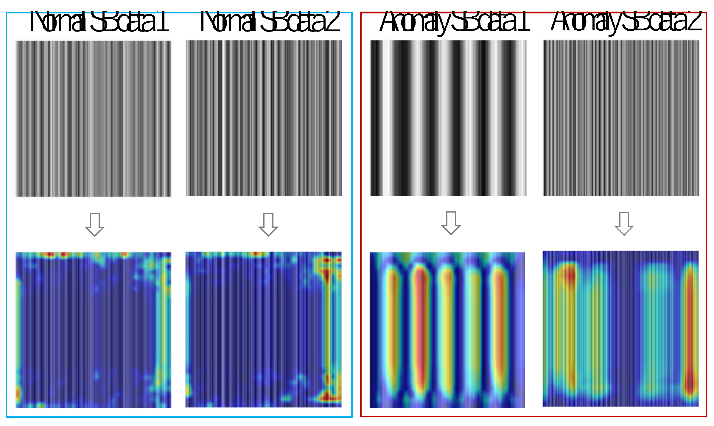

Table 1.
Labels and number of sound blocks for training, validation and test.
| Label | Training | Validation | Test |
|---|---|---|---|
| B13S_S600 | 1600 | 200 | 200 |
| B13S_S1700 | 1600 | 200 | 200 |
| TSL-360CNC_S500 | 1600 | 200 | 200 |
| TSL-360CNC_1000 | 1600 | 200 | 200 |
| TSL-360CNC_S1500 | 1600 | 200 | 200 |
| TSL-360CNC_S2000 | 1600 | 200 | 200 |
| Band-Saw | 1600 | 200 | 200 |
| Milling-Machine | 1600 | 200 | 200 |
| Lathe | 1600 | 200 | 200 |
Table 2.
Structural parameters of 1D CNN (T: Time series data, C: Channel).
| Type | Activation | Parameters |
|---|---|---|
| Sequence Input | 1(T) | - |
| 1D Convolution | 1(T)×32(C) | Weights:5×1×32, Bias:1× 32 |
| ReLU | 1(T)×32(C) | - |
| Normalization | 1(T)×32(C) | Offset:1×32, Scale:1×32 |
| 1D Convolution | 1(T)×64(C) | Weights:5×32×64, Bias:1×64 |
| ReLU | 1(T)×64(C) | - |
| Normalization | 1(T)×64(C) | Offset:1×64, Scale:1×64 |
| Glb. Avg. Pooling | 1(T)×64(C) | - |
| Fully Connected | 9(C) | Weights:9×64, Bias:9×1 |
| Softmax | 9(C) | - |
Table 3.
Max and mean values of MSE in giving nine kinds of test SB data to the trained AE. Note that the SB data of Band-Saw was used to train the AE.
Table 3.
Max and mean values of MSE in giving nine kinds of test SB data to the trained AE. Note that the SB data of Band-Saw was used to train the AE.
| Label | MSE loss (Max) |
MSE loss (Mean) |
Number of misclassified |
|---|---|---|---|
| B13S_S600 | 0.03324 | 0.02738 | 0/300 |
| B13S_S1700 | 0.05668 | 0.02830 | 0/300 |
| TSL-360CNC_S500 | 0.00431 | 0.00250 | 1/300 |
| TSL-360CNC_1000 | 0.00562 | 0.00374 | 1/300 |
| TSL-360CNC_S1500 | 0.00730 | 0.00482 | 1/300 |
| TSL-360CNC_S2000 | 0.01077 | 0.00792 | 1/300 |
| Band-Saw | 0.00121 | 0.00099 | 0/300 |
| Milling-Machine | 0.02555 | 0.02159 | 0/300 |
| Lathe | 0.01447 | 0.01068 | 0/300 |
Table 4.
Labels and number of sound blocks for training and testing an FCDD model.
| Label | Machine Tool | Training | Test |
|---|---|---|---|
| Normal | Band-Saw | 30 | 300 |
| Anomaly | B13S_S600 | 30 | 300 |
| Anomaly | B13S_S1700 | 30 | 300 |
| Anomaly | TSL-360CNC_S500 | 30 | 300 |
| Anomaly | TSL-360CNC_1000 | 30 | 300 |
| Anomaly | TSL-360CNC_S1500 | 30 | 300 |
| Anomaly | TSL-360CNC_S2000 | 30 | 300 |
| Anomaly | Milling-Machine | 30 | 300 |
| Anomaly | Lathe | 30 | 300 |
Table 5.
Classification result of test SBs by SB-based FCDD model (threshold=1.0), in which it is assumed that the sound of Band-Saw is normal and other sounds are anomaly.
Table 5.
Classification result of test SBs by SB-based FCDD model (threshold=1.0), in which it is assumed that the sound of Band-Saw is normal and other sounds are anomaly.
 |
Disclaimer/Publisher’s Note: The statements, opinions and data contained in all publications are solely those of the individual author(s) and contributor(s) and not of MDPI and/or the editor(s). MDPI and/or the editor(s) disclaim responsibility for any injury to people or property resulting from any ideas, methods, instructions or products referred to in the content. |
© 2025 by the authors. Licensee MDPI, Basel, Switzerland. This article is an open access article distributed under the terms and conditions of the Creative Commons Attribution (CC BY) license (http://creativecommons.org/licenses/by/4.0/).
Copyright: This open access article is published under a Creative Commons CC BY 4.0 license, which permit the free download, distribution, and reuse, provided that the author and preprint are cited in any reuse.


