Submitted:
20 August 2025
Posted:
22 August 2025
You are already at the latest version
Abstract
Modeling stock returns and option prices in the presence of jumps remains a central challenge in financial economics. This paper employs a novel score-driven GARCH-jump model to analyze SSE 50 ETF returns and option pricing. The main findings are as follows. First, we use 50 ETF spot returns to estimate historical volatility and jump intensity, and find that the SDSDJ (Score-driven separate dynamic jumps) model significantly outperforms conventional GARCH-jump models in model fitting. Second, we evaluate both in-sample and out-of-sample pricing performance using 50 ETF options data, and find that the SDSDJ model achieves the lowest in-sample pricing error among all benchmarks, while its simplified variant — the SDJ (Score-driven jumps) model — delivers the most accurate out-of-sample results. Third, the superior pricing performance of both models is robust across different levels of moneyness and days-to-maturity (DTM).
Keywords:
SSE 50 ETF option
; score-driven time series models
; option pricing
; jumps
MSC: 62M10; 91B84; 91G20
1. Introduction
Modeling sudden jumps in asset prices is a critical topic in finance. Jumps — typically refer to large, abrupt price changes due to significant news — help explain why asset returns often have fat-tailed distributions and why option implied volatilities exhibit pronounced “smiles”. Empirical evidence in the developed markets such as the U.S. market shows that jumps, while infrequent, can account for a non-trivial share of return variability (on the order of of total variance [1]). In emerging markets such as China, price fluctuations tend to be even more extreme, and existing studies document episodes of abnormal jumps and higher overall volatility than in mature markets [2]. These characteristics make accurate jump modeling particularly important for the Chinese stock market, as it deepens our understanding of return dynamics and improves option valuation in this market.
The Chinese stock market did not introduce exchange-traded equity options until 2015, when the Shanghai Stock Exchange launched the SSE 50 ETF option. Since then, the Chinese option market has expanded rapidly: By 2021, the average daily trading volume reached approximately 2.6 million contracts, making the SSE 50 ETF option one of the most actively traded ETF options. The annual trading volume increased from about 23 million contracts in 2015 to more than 300 million in 2024, reflecting the growing demand for hedging, arbitrage, and speculative activities. In particular, the introduction of SSE 50 ETF options has also impacted the underlying market. For example, Arkorful et al. [3] find that the introduction of these options significantly decreases the volatility of the SSE 50 ETF itself, as the options trading attracts informed traders and improves the flow of information on the spot market. This rapid development of the Chinese option market provides a rich data source and a timely opportunity to study return-jump modeling and option pricing under a new market regime.
Despite the rapid growth of the SSE 50 ETF spot and option markets, most empirical research on return and option modeling focuses on U.S. indices (such as the S&P 500). The Chinese market differs in several important ways which warrantsants a dedicated investigation [4,5]. First, the Chinese equity market is dominated by retail investors and is periodically shaped by regulatory interventions, resulting in regime shifts and clusters of large price movements. Second, capital controls and other restrictions can cause liquidity shocks around policy events, for example, the daily price limits may also induce discontinuities. Third, the SSE 50 ETF options are physically delivered contracts that are adjusted for dividends — a feature uncommon in standard index options. Besides, the number of available strike prices is limited, and the cost of short-selling the underlying assets is much higher than in U.S. markets. Finally, implied volatility in the SSE 50 ETF options market is generally higher than in the U.S., and its volatility smile exhibits a right skew—where deep in-the-money calls and out-of-the-money puts are relatively expensive. This contrasts with the typically left-skewed smirk observed in U.S. index options. These distinctive market characteristics highlight the limitations of traditional models and motivate the development of context-specific approaches to volatility and jump modeling in the Chinese equity market.
A wide range of models have been developed to capture asset volatility dynamics in both continuous and discrete time. The classic continuous-time framework, such as the stochastic volatility model proposed by Black and Scholes [6] and Heston [7] laid the theoretical foundation for option pricing under diffusion processes. On the discrete-time side, GARCH models have been proven to be very successful in capturing time-varying volatility. Building on this success, Duan [8] pioneered the GARCH option pricing model, showing that a GARCH-based approach can parsimoniously track changing volatility and even explain certain systematic pricing biases of the Black–Scholes model. Subsequently, Heston and Nandi [9] derived a closed-form option valuation formula for a GARCH process, providing the first convenient analytical pricing formula for a stochastic volatility model calibrated entirely on observable returns.
However, empirical findings document that asset returns are occasionally hit by large jumps triggered by news or unexpected events. A growing body of literature links jumps to the arrival of big news (e.g., [10,11,12,13,14]). For instance, using an extensive news dataset, Jeon et al. [14] show that stock price jumps (in both frequency and size) are strongly related to news flows and their content, especially for firms with high media coverage. These evidences reinforce the view that jumps are not merely statistical outliers but are often tied to fundamental information events. To accommodate these discontinuities in returns, researchers have extended volatility models to include jump components. In discrete time, numerous GARCH-jump models have been proposed for equities and exchange rates (e.g., [10,15]), where the return innovation has a mixture of a GARCH-driven continuous part and a jump-driven discontinuous part. These models have also been adapted to option pricing: for example, Duan et al. [16] develop approximation methods for GARCH–jump models, Christoffersen et al. [17] estimate a model with time-varying jump intensity to price S&P 500 options. A consistent finding in the literature is that incorporating jumps improves pricing accuracy, and models with dynamic jumps outperform their static counterparts. For example, Christoffersen et al. [18] and Christoffersen et al. [17] verify that models allowing for jumps (especially with time-varying intensity) outperform those assuming purely continuous fluctuations, and Hsieh and Ritchken [19] obtain similar evidence when comparing GARCH models with and without jumps.
While GARCH-based models have been very useful, they rely on certain heuristics (e.g. using lagged squared returns) to update volatility, which can pose robustness issues. This has led to the development of score-driven volatility models (also known as dynamic conditional score models) by Creal et al. [20] and Harvey [21]. Score-driven models take a different approach: the time-varying parameters (such as volatility or jump intensity) are updated each period according to the score of the log-likelihood — essentially the first moment of the predictive distribution — rather than ad-hoc functions of past residuals. This generalized filtering mechanism ensures that the updates optimally incorporate new information in the same way the likelihood would. An attractive feature of score-driven models is their flexibility and consistency with observation density: they naturally accommodate heavy tails and time-varying higher moments by design. In view of this, Ballestra et al. [22] recently proposed a score-driven GARCH–jump model, where both the conditional variance and the conditional jump intensity evolve according to auto-regressive updates driven by scaled score innovations. Their empirical application to S&P 500 returns and options demonstrates an excellent in-sample fitting and significant out-of-sample improvements, surpassing traditional GARCH-jump benchmarks. In particular, the score-driven model can accurately capture returns’ jump clustering and volatility dynamics, resulting in more reliable pricing of the S&P 500 options. These results suggest that score-driven jump models can offer a powerful platform for option valuation.
In contrast to the extensive U.S. literature, relatively few studies have examined volatility modeling and option pricing in the Chinese market. Notable exceptions include Huang et al. [5], who recently compare discrete-time models on SSE 50 ETF options. They find that models incorporated realized volatility measures outperform standard GARCH models based on daily returns. Another study by Yang [23] introduced a GARCH option pricing model that includes a double-exponential jump component (following the framework of Kou and Wang [24]) to allow separate modeling of upward and downward jumps. This approach acknowledges the asymmetric impact of good news versus bad news on prices. However, to the best of our knowledge, the performance of score-driven GARCH-jump models has not yet been investigated for the Chinese stock market. In light of the unique market characteristics discussed above and the good performance of score-driven models in other contexts, it is natural to investigate whether these models can enhance return filtering and option pricing in the SSE 50 ETF market.
This paper employs a novel score-driven GARCH-jump model to fit SSE 50 ETF returns and option pricing. The main findings are as follows. First, we use 50 ETF spot returns to estimate historical volatility and jump intensity, and find that the SDSDJ (Score-driven separate dynamic jumps) model significantly outperforms conventional GARCH-jump models in model fitting. Second, we evaluate both in-sample and out-of-sample pricing performance using 50 ETF options data, and find that the SDSDJ model achieves the lowest in-sample pricing error among all benchmarks, while its simplified variant — the SDJ (Score-driven jumps) model — delivers the most accurate out-of-sample results. Third, the superior pricing performance of both models is robust across different levels of moneyness and days-to-maturity (DTM).
The remainder of this article is organized as follows. Section 2 provides the data and an overview of the SSE 50 ETF options market. Section 3 introduces the methodology, including the SDSDJ and SDJ models, used in this paper. Section 4 presents and discusses the empirical results. Section 5 concludes.
2. The Data and Features of the SSE 50 ETF Option Market
The underlying asset of the SSE 50 ETF options is the 50 ETF issued by Hua Xia Fund Asset Management Company. Covering the 50 largest high-liquidity blue-chip stocks listed on the SSE, the SSE 50 ETF accounted for approximately of the total market value (i.e., over trillion RMB) of all equity ETFs in China by the end of 2024. In this study, we use the daily returns of SSE 50 ETF from February 23, 2005, to October 28, 2024, and the daily settlement prices of SSE 50 ETF option contracts from February 9, 2015, to October 28, 2024, as the sample. The data are sourced from the Wind Database, which is a reliable and widely used financial database in China. Figure 1 (a) shows the log-return time series of the 50 ETF, and Panel A of Table 1 gives the descriptive statistics. Apparently, we can find that the 50 ETF returns are highly volatile, there exists evidence of time-varying jumps, and jumps tend to cluster over time. Therefore, the returns are characterized by a sharp peak and fat tails.
The 50 ETF option was introduced on 9 February 2015 as a European-style, physically settled option written on the 50 ETF. The basic contract terms are provided in Table 2. As illustrated in Figure 1 (b), both daily trading volume and open interest increased dramatically from 2015 to 2024. Panel A of Table 3 lists the proportion of trading volume by option category. We can find that: First, ATM and OTM options account for more than of total trading volume, while ITM options account for less than . Second, short- and medium-term options with DTM of less than 60 days comprise over of trading volume, whereas long-term options account for less than . Therefore, in line with the statistics and consistent with the literature (e.g., [22]), we restrict our selection to ATM and OTM options with maturities of up to one year (250 days) for pricing, as shown in Panel B of Table 1.
Compared to their U.S. counterparts, SSE 50 ETF options exhibit several notable differences in contract specifications, regulatory practices, and market behavior. First, the number of available strikes is limited. At inception, the 50 ETF options offered only five strikes (one ATM, two OTM, and two ITM), which expanded to nine strikes (one ATM, four OTM, and four ITM) by early 2018. New strikes are added upon dividend adjustments, and seventeen such adjustments have been made since the product’s launch.
Second, option contracts are adjusted when dividends are paid on the underlying ETF. Specifically, if the ex-dividend price of the ETF is S and the cash dividend is d, the adjustment provides each holder with new contracts at a strike price of for each original contract at strike K. This leads to the following pricing identity:
This mechanism effectively shields option holders from dividend-induced price drops — a feature not standard for index options such as SPX.
Third, the Chinese market experiences higher price volatility [5]. From February 2015 to December 2024, the average realized 10-day volatility of the 50 ETF was approximately , compared to about for the S&P 500 (SPX). Moreover, by February 2018, the volatility premium (defined as VIX minus realized volatility) for the 50 ETF was approximately higher than that of SPX options.
Finally, the smile curve of 50 ETF put options exhibits a right-skewed structure, while that of call options is approximately symmetric, as shown in Panel B of Table 3. In the SSE 50 ETF market, the implied volatility of deep-in-the-money (DITM) put options is higher than that of at-the-money (ATM) and out-of-the-money (OTM) puts. This pattern contrasts sharply with the U.S. options market, where OTM put options tend to have higher implied volatility than ITM options — resulting in a left-skewed smile.
These observations underscore fundamental differences between the Chinese and U.S. options markets, suggesting that pricing models calibrated for the U.S. may not be directly applicable to the Chinese context.
3. The Methodology
3.1. The SDSDJ and SDJ Models
We first introduce the SDSDJ option pricing model. Let denote the daily closing price series of SSE 50 ETF, then the log-return is , including the dividend . Following Christoffersen et al. [17], we use affine building blocks to model the log-return as follows:
where shocks to returns are generated by the normal component and the jump component , r is the risk-free rate, and are risk premiums of the normal component and jump component of shocks, respectively, is the conditional variance, is the jump intensity, and act as compensators to the normal and jump components, respectively, ensuring that when taking conditional expectations of returns, we have
Specifically, is a Gaussian random variable, and is defined as a compound Poisson process:
where is the number of jumps arriving between times and t, is a sequence of independent and identically distributed normal random variables, . Following Christoffersen et al. [17] and Ballestra et al. [22], we can obtain the log-likelihood function of the log-return series as follows:
Our primary concern is on understanding how the conditional variance () and jump intensity () evolve over time — an iterative process that fundamentally distinguishes various GARCH-type models from one another. We specify the conditional variance () and the conditional jump intensity () using a score-driven model [20,21],
where and are the logarithms of and , and are score functions, and are parameters to be estimated. We use the exponential link function to keep the variance and jump intensity always positive.
The usage of score functions (i.e., and ) into the GARCH-type option pricing model is the key innovation of the SDSDJ model. We consider the score of the predictive distribution:
By differentiating Equation (5) with respect to and and substituting the result into Equation (7), we can get the unscaled score functions and . However, the unscaled score functions are unbounded, which may lead to explosive trajectories, making the evaluation of option prices infeasible. Following Ballestra et al. [22], we add a scale factor to and , the final score functions (i.e., and ) are as follows,
where
3.2. Option Valuation
Equation (6) can be used to model the conditional volatility and jump intensity of the log-return series of SSE 50 ETF, as an alternative to the traditional GARCH model. However, in order to price the SSE 50 ETF options, risk neutralization is needed to convert the physical measure (real-world measure, ) to the risk-neutral measure (equivalent martingale measure, ). Following Christoffersen et al. [17] and Ballestra et al. [22], the log-return process and the iterative process under -measure are as follows:
where , is a compound Poisson process, whose jump intensity is and jump size follows , in which is the equivalent martingale measure (EMM) coefficient that capture the wedge between the physical and the risk-neutral measure. Under the -measure, and are the score functions given by
where
Using Equation (10) and (11), we can numerically calculate the SSE 50 ETF option price based on the current underlying price, risk-free rate (set to 0 following Ballestra et al. [22]), date-to-maturity (DTM), strike price and option type (call or put) as follows:
where is the option price, is the payoff of the option at maturity, is the information set available up to time t.
Fitting a dynamic model to a panel of option prices could be really challenging, especially when the goal is to jointly estimate parameters using both returns and option prices [22]. Since it is important to consider both sources of information, we define a suitably weighted log-likelihood function that incorporates both the daily time series of log-returns and the panel of option contracts. While the log-likelihood for the daily returns, , is already provided in Equation (5), modeling the option pricing errors requires additional assumptions. Formally, if we have N option prices, the option pricing error for the i-th contract, , for , is defined as the relative implied volatility loss function:
where and denote the market and the model implied volatilities of the i-th option, respectively, which are computed according to the popular Black-Scholes model. Then, following Christoffersen et al. [17] and Ornthanalai [25], the likelihood associated with the error on implied volatility is computed through using a Gaussian specification:
It is important to note that the number N of data points available for the option panel is different from the number T of daily returns. Therefore, according to Christoffersen et al. [17] and Ornthanalai [25], to assign an equal weight to returns and option prices, we consider the following weighted joint (total) log-likelihood:
To assess the performance of the option pricing models, we follow Ballestra et al. [22], and employ the (percentage) implied volatility root mean square error:
where N is the total number of option prices considered while and denote the market and the model implied volatilities of the i-th option, respectively.
It is remarked that the SDJ model is a special case of the SDSDJ model, where the jump intensity is a constant () rather than time-varying (). Both models share the same log-likelihood function, score functions, and iterative procedure under both the physical () and risk-neutral () measures.
3.3. Benchmark Models
To demonstrate the advantage of the score-driven GARCH-jump model, the Black-Scholes ([6]), Heston & Nandi GARCH ([9]), GARCHJ (GARCH model with jumps [18]) and DVSDJ (dynamic volatility separate dynamic jumps [17]) option pricing models are chosen as benchmark models.
Since the Black-Scholes model is so well-known and widely used, we will not introduce it in this paper. First, the Heston & Nandi GARCH model uses a closed-form solution as follows rather than numerical methods:
where C is the model-implied price of call options, S is the current price of the underlying asset, is an operator taking the real part of a complex number, r is the risk-free rate, is the date-to-maturity, and is the conditional volatility. The price of put options can be calculated by the put-call parity.
Second, the GARCHJ model incorporates static jumps (i.e., Poisson process) into the GARCH option pricing model, whose return process is the same as Equation (2) and the iterative process is as follows:
where is the conditional variance, and are the normal and jump component of shocks for returns, respectively, are parameters to be estimated.
Last, the DVSDJ model is the generalized version of the GARCHJ model, where the jump intensity varies over time. The return process of the DVSDJ model is the same as Equation (2), and the iterative process is as follows:
where is the conditional variance, is the dynamic jump intensity, and are the normal and jump component of shocks respectively, are parameters to be estimated.
4. Empirical Results
4.1. In-Sample Fitting of Spot Returns
We use different GARCH-type models (H-N GARCH, GARCHJ, SDJ, DVSDJ, and SDSDJ) to filter the conditional volatility and jump intensity of the 50 ETF spot returns. Since different models imply different conditional volatility and jump intensity for the same market, our objective is to identify which model achieves superior in-sample fitting.
Table 4 presents the maximum likelihood estimation results for these models. First, three different criteria — log-likelihood value, AIC, and BIC — are used to evaluate model fitting. From the table, we can find that, among all GARCH-type models, the novel SDSDJ model achieves the highest log-likelihood and the lowest AIC and BIC. Interestingly, the SDJ and DVSDJ models perform even worse than the plain vanilla Heston-Nandi GARCH model. Therefore, we demonstrate that score-driven GARCH-jump models provide better in-sample fitting. Second, as shown in the table, we find that none of the GARCH-type models produce significant coefficients estimates for , whereas the S&P 500 market exhibits a significant jump risk premium (e.g., ; see [22]). However, is significantly positive across models, indicating that investors are compensated for bearing the normal component of risk. Third, the jump size (denoted by ) of log-returns in the 50 ETF market is relatively small. As shown in the table, although all estimated values are negative — reflecting negatively skewed returns — their absolute magnitudes are small, in contrast to jump sizes of around observed in the S&P 500 market. Last, similar to the S&P 500 market, there exists significant interaction between the normal and jump components for the SSE 50 ETF market. The relative magnitudes of and reflect the interaction between jump intensity and conditional variance. If , the interaction is considered significant [22], which is also confirmed by the estimates in the table.
Figure 2 plots the filtered conditional volatility for different models. As illustrated in Panel (a)-Panel (e), the 50 ETF has experienced two episodes of extreme volatility: the 2008 financial crisis and the 2015 Chinese stock market crash. Although the traditional GARCH model captures all three market shocks, its volatility peaks are not pronounced, exhibiting a relatively smooth pattern, and the same applies to the static GARCHJ model (Panel (b)). In contrast, Panel (d) shows that the SDJ model provides more significant peaks in modeling the conditional volatility of the 50 ETF, and the same holds for the SDSDJ model (Panel (e)).
Figure 3 presents the filtered jump intensity for different GARCH-jump models. Clearly, the dynamic models (i.e., DVSDJ and SDSDJ) provide more significant peaks than the static models (i.e., GARCHJ and SDJ). One possible reason is that static models use constant jump intensities, making it difficult to distinguish between high- and low-volatility trading days. However, the GARCH-jump models with dynamic jump models provide better estimates of the number of posterior jumps associated with several market crises.
Finally, we propose a general criterion for evaluating the quality of volatility models: to what extent can the model strip out the predictable part of the log-return and assign the truly random and unpredictable part into the normal component (). Time series models with stronger explanatory power should yield values that are closer to a standard normal distribution. Figure 4 illustrates the Q-Q plots of the normal innovation for each GARCH model. As shown in the figure, the traditional GARCH-type models deviate significantly from the standard normal distribution beyond , while the SDSDJ model closely approximates a standard normal distribution within .
4.2. Out-of-Sample Analysis
To evaluate the predictive performances of the novel SDSDJ model and its rival models, we follow Ballestra et al. [22] and forecast the 5% and 1% Value-at-Risk (VaR) from one to five days ahead. We evaluate the predictive performance of these models across different crisis periods by partitioning the dataset into five subperiods and conducting separate out-of-sample analyses: January 2005 – August 2009 (capturing the 2008 global financial crisis), August 2009 – December 2012 (a relatively stable period), January 2013 – December 2017 (including the 2015 Chinese stock market crash), January 2018 – December 2022 (covering the 2020 COVID-19 pandemic), and December 2022 – November 2024.
For each period, we estimate model parameters utilizing a rolling window corresponding to of the total number of days in that period. Initially, we calibrate the models using the first of daily total returns from the SSE 50 ETF, reserving the remaining data for out-of-sample evaluations. Subsequently, for each day within the out-of-sample dataset, we re-estimate the parameters employing the latest daily return observations and generate forecasts for horizons ranging from one to five days ahead.
Specifically, for the SDSDJ model, at each forecast date , we generate simulated return paths for , with , based on the return specification in Equation (2). This involves randomly generating the innovations and , with and evolving according to Equation (6). The GARCHJ, DVSDJ, and SDJ models follow analogous simulation procedures. We then calculate the Value at Risk (VaR) at significance levels of and by determining empirical quantiles from the simulated outcomes of . Following Creal et al. [20], we evaluate VaR forecast accuracy through the proportion-of-failures test proposed by Kupiec [26]. The null hypothesis for this out-of-sample test is defined as : The probability of model prediction failure equals. Consequently, if the null hypothesis is rejected, it implies the model lacks significant predictive capability.
Table 5 reports the result of the likelihood ratio test. The same model performs differently at high and low quantiles. Market conditions are also crucial for model performance. This finding provides strong empirical support for our model selection.
During the 2008 global financial crisis period (Panel A), at the level, the SDJ and SDSDJ models exhibit superior performance, each with only one rejection. In contrast, the GARCHJ and DVSDJ models are rejected five times each. At the level, all models show similar performance. Interestingly, during the relatively stable period (Panel B), the SDSDJ model performs best at but worst at , while the GARCHJ model exhibits the opposite tendency. During the 2015 Chinese stock market crash period (Panel C), all models show relatively strong performance at the level, but perform poorly at the level. The COVID-19 pandemic (Panel D) shows a pattern similar to the 2008 crisis: SDSDJ performs best at , whereas GARCHJ performs best at . In the most recent period (Panel E), the SDSDJ model performs well at both the and levels.
Overall, these results suggest that the novel SDSDJ and SDJ models capture the extreme tail (e.g., ) of the conditional return distribution very effectively. By contrast, traditional GARCH-type models are well-suited to modeling non-extreme returns (e.g., ) but provide a considerably weaker out-of-sample fit for extreme losses.
4.3. In-Sample Option Valuation
The GARCH-type models under -measure can be used to model the conditional volatility and jump intensity of spot returns, while those under -measure can be used to price options. We apply several risk-neutralized GARCH-type models, including the novel SDSDJ and SDJ, to price the 50 ETF options from February 23, 2015, to December 20, 2024. Table 6 presents the joint MLE estimation results. Similar to the MLE estimation results for spot returns, the SDSDJ model achieves the highest log-likelihood value and the lowest AIC and BIC among all GARCH-type models. However, we find that the DVSDJ model performs very poorly over the time horizon, with a log-likelihood of only — lower than that of the SDSDJ model. This result supports the idea that incorporating score dynamics improves the performance of GARCH-jump models in option pricing. Furthermore, the estimates of in the table indicate that the risk premium associated with the jump component is significantly positive, the jump sizes are all negative, and the values of lie between 0 and 1. These findings are consistent with those of [17,18,22,25].
We also employ the criterion of IVRMSE to evaluate the performance of the four competing models. Table 7 reports the in-sample IVRMSE for different option pricing models, both overall and across various moneyness and maturities. Panel A indicates that, overall, the SDSDJ model performs best, with an IVRMSE of only , followed by the SDJ model () and the GARCHJ model (), while the DVSDJ model performs the worst (). Panel B shows that the pricing errors for out-of-the-money options are generally higher than those for at-the-money options. Panel C reveals that short-term options tend to have higher pricing errors than long-term ones. As DTM increases, IVRMSE decreases — for example, the GARCHJ model performs better in the long term () than in the short term (), and similar patterns are observed for the other models. Our primary concern is whether the novel SDSDJ model outperforms most traditional GARCH-type models across different maturities and moneyness levels. The SDSDJ model demonstrates robust and consistently superior performance, with IVRMSE ranging from to across maturities and from to across moneyness categories. It therefore confirms the robustness of its performance with respect to the option term structure.
4.4. Out-of-Sample Option Valuation
We also conduct out-of-sample analyses. For each year, all option contracts from the first half of the year are used for training to estimate the optimal parameters. These parameters are then applied to price option contracts in the second half of that year, and the model-implied volatility is obtained using the classic Black-Scholes formula. By comparing the model implied volatility with the market implied volatility, we compute the out-of-sample IVRMSE for each model.
Table 8 reports the out-of-sample IVRMSE for different option pricing models, both overall and across various moneyness and maturities. Panel A indicates that the SDJ model yields the lowest overall IVRMSE, while the SDSDJ model performs poorly out of sample. This may be due to the larger number of parameters, which can lead to overfitting and, consequently, weaker out-of-sample performance. In contrast, more parsimonious models (such as Black-Scholes and SDJ) demonstrate greater stability. Panels B through D present results when the options sample is sorted for year, maturity, and DTM, respectively. We have the following discoveries. First, higher market volatility is associated with worse model performance. For example, in 2020 and 2024, the IVRMSE for all models exceeds , while in 2022 and 2023 it can be as low as (for the SDJ model). This substantial variation highlights the sensitivity of GARCH-type models to market conditions. During crisis periods, the performance of option pricing models generally deteriorates; however, the SDJ model remains the most robust among them. Second, pricing accuracy is higher for at-the-money options compared to deep out-of-the-money options, and the SDJ model performs best across all moneyness categories. Finally, all models exhibit better performance in pricing long-term options, which is consistent with the in-sample findings.
In summary, the empirical results on option valuation in this section demonstrate that the novel score-driven models outperform traditional approaches — including both GARCH-type models and the classic Black-Scholes model — in both in-sample and out-of-sample analyses.
5. Conclusions
This paper employs a novel score-driven GARCH-jump model to analyze SSE 50 ETF returns and option pricing. Our analysis yields several key findings:
(1) The SDSDJ model achieves the highest log-likelihood and the lowest AIC and BIC values, indicating its superior in-sample fitting to the underlying ETF return series. This model effectively captures both time-varying volatility and jump dynamics by utilizing score-driven filters.
(2) The Kupiec’s likelihood ratio test shows that while the traditional GARCHJ model performs relatively well during stable periods, the SDSDJ and SDJ models consistently exhibit superior accuracy in capturing extreme losses, particularly during turbulent market conditions. These findings highlight the robustness of the SDSDJ framework in modeling fat-tailed return distributions and its practical relevance for risk management under stress scenarios.
(3) The option pricing analysis shows that the SDSDJ model achieves the best in-sample performance across all GARCH-type models, and they have robust pricing accuracy across moneyness and maturities. However, its out-of-sample performance is less stable — likely due to overfitting, while its simplified variant — the SDJ model — delivers the most accurate out-of-sample results. These results imply a trade-off between model flexibility and generalizability, suggesting that while dynamic models like SDSDJ may offer better in-sample fits, more parsimonious structures such as SDJ are better suited for practical option pricing under varying market conditions.
In summary, the SDSDJ and SDJ models provide a unified framework for return modeling and option pricing, demonstrating robustness across different market conditions. These findings have important implications for regulators and practitioners, who may consider adopting novel score-driven GARCH-type models for return modeling and option pricing. This study contributes to the literature on financial modeling in the Chinese equity markets and option pricing by evaluating the empirical performance of such novel score-driven models.
Author Contributions
Conceptualization, M.S. and C.Z.; methodology, M.S. and C.Z.; software, M.S.; validation, M.S., C.Z. and W.H.; formal analysis, M.S. and C.Z.; resources, C.Z, Q.C. and W.H.; data curation, M.S.; writing—original draft preparation, M.S.; writing—review and editing, C.Z., Q.C. and W.H.; supervision, C.Z. and W.H. All authors have read and agreed to the published version of the manuscript.
Funding
This research received no external funding.
Institutional Review Board Statement
Not applicable.
Informed Consent Statement
Not applicable.
Data Availability Statement
The data presented in this study are available on request from the corresponding author.
Acknowledgments
Zhang’s research is jointly supported by the Humanity and Social Science Youth Foundation of Ministry of Education of China (Grant No. 18YJC790210), the Innovation and Talent Base for Digital Technology and Finance (Grant No. B21038), and the Fundamental Research Funds for the Central Universities, Zhongnan University of Economics and Law (Grant No. 2722024BY008;2722023EJ002). Härdle’s research is supported through the European Cooperation in Science & Technology COST Action grant CA19130 – Fintech and Artificial Intelligence in Finance – Towards a transparent financial industry; the project “IDA Institute of Digital Assets”, CF166/15.11.2022, contract number CN760046/23.05.2024 financed under the Romania’s National Recovery and Resilience Plan, Apel nr. PNRR-III-C9-2022-I8; and the Marie Sklodowska-Curie Actions under the European Union’s Horizon Europe research and innovation program for the Industrial Doctoral Network on Digital Finance, acronym DIGITAL, Project No. 101119635.; the Yushan Fellowships, TW
Conflicts of Interest
The authors declare that they have no known competing financial interests or personal relationships that could have appeared to influence the work reported in this paper.
Abbreviations
The following abbreviations are used in this manuscript:
| GARCH | Generalized Autoregressive Conditional Heteroskedasticity |
| H-N GARCH | Heston & Nandi GARCH |
| GARCHJ | GARCH with Jumps |
| DVSDJ | Dynamic Volatility with Separate Dynamic Jumps |
| SDJ | Score-Driven Model with Jumps |
| SDSDJ | Score-Driven Model with Separate Dynamic Jumps |
| AIC | Akaike Information Criterion |
| BIC | Bayesian Information Criterion |
| IVRMSE | Implied Volatility Root Mean Squared Error |
| MLE | Maximum Likelihood Estimation |
References
- Huang, X.; Tauchen, G. The relative contribution of jumps to total price variance. J. Financ. Econom. 2005, 3(4), 456–499. [Google Scholar]
- Yang, S. Identifying multiple bubbles and time-varying contagion effect between iron ore and china’s stock markets: a new recursive evolving test. Rom. J. Econ. Forecast 2025, 28(1), 81. [Google Scholar]
- Arkorful, G.B.; Chen, H.; Liu, X.; Zhang, C. The impact of options introduction on the volatility of the underlying equities: Evidence from the Chinese stock markets. Quant. Finance 2020, 20(12), 2015–2024. [Google Scholar] [CrossRef]
- Yue, T.; Gehricke, S.; Zhang, J. E.; Pan, Z. How Do Chinese Option-Traders “smirk” on China: Evidence from SSE 50 ETF Options. Working paper 2019. [Google Scholar]
- Huang, Z.; Tong, C.; Wang, T. Which volatility model for option valuation in China? Empirical evidence from SSE 50 ETF options. Appl. Econ. 2019, 52(17), 1866–1880. [Google Scholar] [CrossRef]
- Black, F; Scholes, M. The pricing of options and corporate liabilities. J. Political Econ. 1973, 81(3), 637–54. [Google Scholar] [CrossRef]
- Heston, S. L. A closed-form solution for options with stochastic volatility with applications to bond and currency options. Rev. Financ. Stud. 1993, 6(2), 327–43. [Google Scholar] [CrossRef]
- Duan, J. C. The GARCH option pricing model. Math. Finance 1995, 5(1), 13–32. [Google Scholar] [CrossRef]
- Heston, S. L.; Nandi, S. A closed-form GARCH option valuation model. Rev. Financ. Stud. 2000, 13(3), 585–625. [Google Scholar] [CrossRef]
- Maheu, J. M.; McCurdy, T. H. News arrival, jump dynamics, and volatility components for individual stock returns. J. Finance 2004, 59(2), 755–793. [Google Scholar] [CrossRef]
- Zhang, C.; Liu, Z.; Liu, Q. Jumps at ultra-high frequency: Evidence from the Chinese stock market. Pac. Basin Finance J. 2021, 68, 101420. [Google Scholar] [CrossRef]
- Zhang, C.; Chen, H.; Peng, Z. Does Bitcoin futures trading reduce the normal and jump volatility in the spot market? Evidence from GARCH-jump models. Finance Res. Lett. 2022, 47, 102777. [Google Scholar] [CrossRef]
- Zhang, C.; Ma, H.; Liao, X. Futures trading activity and the jump risk of spot market: Evidence from the bitcoin market. Pac. Basin Finance J. 2023, 78, 101950. [Google Scholar] [CrossRef]
- Jeon, Y.; McCurdy, T. H.; Zhao, X. News as sources of jumps in stock returns: Evidence from 21 million news articles for 9000 companies. J. Financ. Econ. 2022, 145(2), 1–17. [Google Scholar] [CrossRef]
- Vlaar, P. J.; Palm, F. C. The message in weekly exchange rates in the European monetary system: mean reversion, conditional heteroscedasticity, and jumps. J. Bus. Econ. Stat. 1993, 11(3), 351–360. [Google Scholar] [CrossRef]
- Duan, J. C.; Ritchken, P.; Sun, Z. Approximating GARCH-JUMP Models, Jump-Diffusion Processes, And Option Pricing. Math. Finance 2006, 16(1), 21–52. [Google Scholar] [CrossRef]
- Christoffersen, P.; Jacobs, K.; Ornthanalai, C. Dynamic jump intensities and risk premiums: Evidence from S&P500 returns and options. J. Financ. Econ. 2012, 106(3), 447–472. [Google Scholar]
- Christoffersen, P.; Jacobs, K.; Ornthanalai, C.; Wang, Y. Option valuation with long-run and short-run volatility components. J. Financ. Econ. 2008, 90(3), 272–297. [Google Scholar] [CrossRef]
- Hsieh, K.; Ritchken, P. An empirical comparison of GARCH option pricing models. Rev. Deriv. Res. 2005, 8, 129–150. [Google Scholar] [CrossRef]
- Creal, D.; Koopman, S. J.; Lucas, A. A dynamic multivariate heavy-tailed model for time-varying volatilities and correlations. J. Bus. Econ. Stat. 2011, 29(4), 552–563. [Google Scholar] [CrossRef]
- Harvey, A. C. Dynamic models for volatility and heavy tails: with applications to financial and economic time series; Cambridge University Press, 2013.
- Ballestra, L. V.; D’Innocenzo, E.; Guizzardi, A. Score-driven modeling with jumps: an application to S&P500 returns and options. J. Financ. Econom. 2023, 22(2), 375–406. [Google Scholar]
- Yang, X. Good jump, bad jump, and option valuation. J. Futures Mark. 2018, 38(9), 1097–1125. [Google Scholar] [CrossRef]
- Kou, S. G.; Wang, H. Option pricing under a double exponential jump diffusion model. Manag. Sci. 2004, 50(9), 1178–1192. [Google Scholar] [CrossRef]
- Ornthanalai, C. Levy jump risk: Evidence from options and returns. J. Financ. Econ. 2014, 112(1), 69–90. [Google Scholar] [CrossRef]
- Kupiec, P. Techniques for verifying the accuracy of risk measurement models. J. Deriv. 1995, 3(2), 73–84. [Google Scholar] [CrossRef]
Figure 1.
Log-return of SSE 50 ETF and trading volumn and open interest of 50 ETF options. (a) The log-return of 50 ETF; (b) trading volumn and open interest of 50 ETF options, where the blue bars represent trading volume (in tens of thousands) and the red line represents open interest (in tens of thousands).
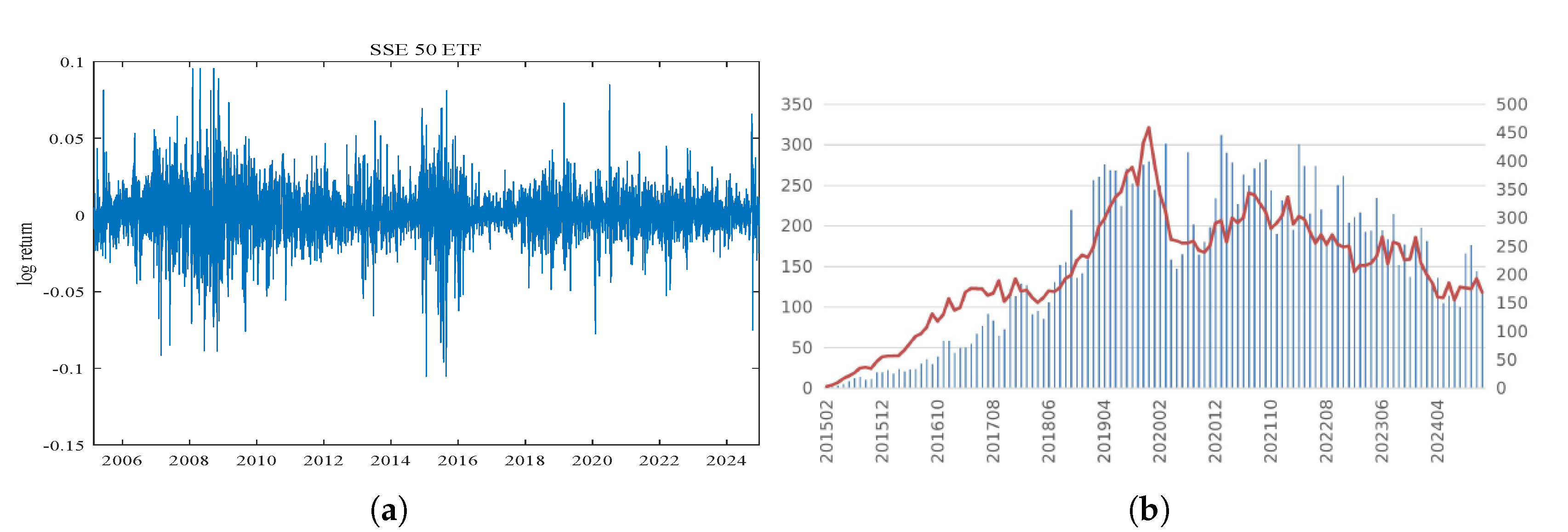
Figure 2.
The figures illustrate the time series plots of filtered conditional volatility. The sample period is from February 23, 2005 to October 28, 2024. (a) Heston & Nandi GARCH model; (b) GARCHJ model; (c) DVSDJ model; (d) SDJ model; (e) SDSDJ model.
Figure 2.
The figures illustrate the time series plots of filtered conditional volatility. The sample period is from February 23, 2005 to October 28, 2024. (a) Heston & Nandi GARCH model; (b) GARCHJ model; (c) DVSDJ model; (d) SDJ model; (e) SDSDJ model.
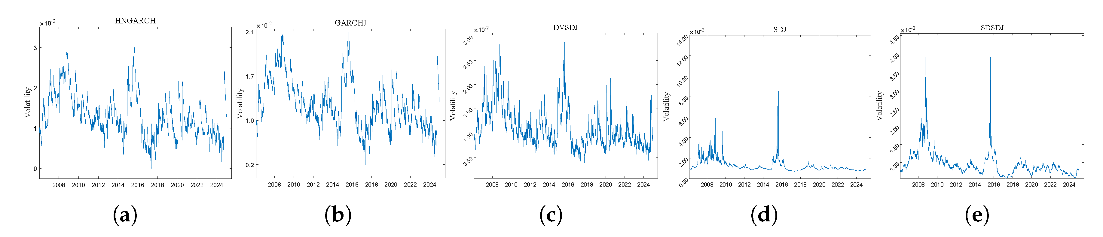
Figure 3.
The figures illustrate the time series plots of filtered jump intensity. The sample period is from February 23, 2005 to October 28, 2024. (a) GARCHJ model; (b) DVSDJ model; (c) SDJ model; (d) SDSDJ model.
Figure 3.
The figures illustrate the time series plots of filtered jump intensity. The sample period is from February 23, 2005 to October 28, 2024. (a) GARCHJ model; (b) DVSDJ model; (c) SDJ model; (d) SDSDJ model.
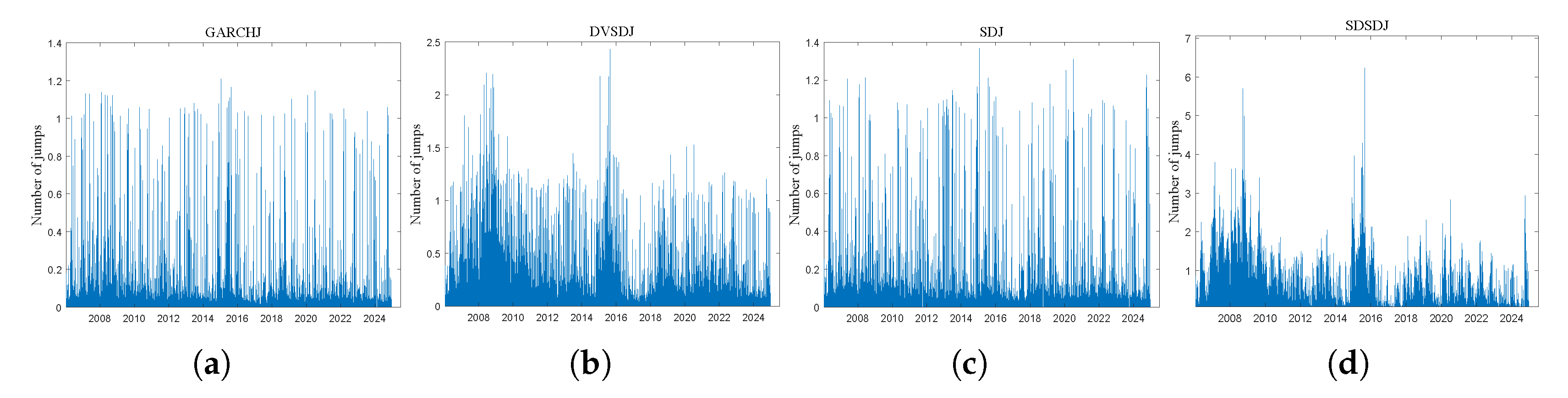
Figure 4.
The figures illustrate the Q-Q plots of the normal innovation . The sample period is from February 23, 2005 to October 28, 2024. (a) Heston & Nandi GARCH model; (b) GARCHJ model; (c) DVSDJ model; (d) SDJ model; (e) SDSDJ model.
Figure 4.
The figures illustrate the Q-Q plots of the normal innovation . The sample period is from February 23, 2005 to October 28, 2024. (a) Heston & Nandi GARCH model; (b) GARCHJ model; (c) DVSDJ model; (d) SDJ model; (e) SDSDJ model.
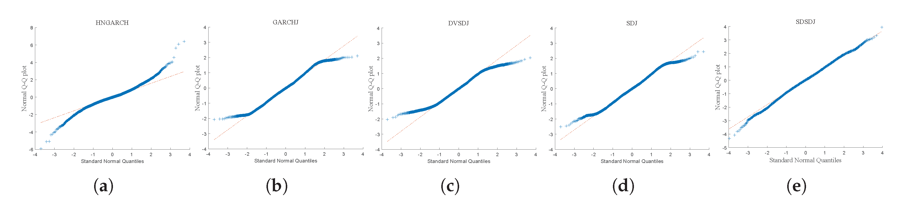

Table 1.
Descriptive statistics.
| Panel A: the daily log-return of SSE 50 ETF | ||||
|---|---|---|---|---|
| Mean | Std. error | Skewness | Kurtosis | |
| SSE 50 ETF | 3.04E-4 | 1.64E-2 | -1.27E-1 | 8.43 |
| Panel B: Number of options | ||||
| DTM | ||||
| Moneyness () | 10–30 | 30–90 | 90–250 | Total |
| <0.9 | 1471 | 2053 | 1030 | 4554 |
| 0.9–1.0 | 3209 | 3441 | 2864 | 9514 |
| 1.0–1.1 | 2800 | 3033 | 2543 | 8376 |
| >1.1 | 1604 | 2066 | 1213 | 4883 |
| Total | 9084 | 10593 | 7650 | 27327 |
1 Notes: The sample period for the SSE 50 ETF is from February 23, 2005, to October 28, 2024, and that for the SSE 50 ETF options is from February 9, 2015, to October 28, 2024. DTM denotes days to maturity, and denotes moneyness, defined as the ratio of the strike price to the spot price.
Table 2.
Basic terms of the SSE 50 ETF option contracts.
| Items | Descriptions |
|---|---|
| Underlying Asset | SSE 50 ETF |
| Option Types | Call options and Put options |
| Exercise Style | European-style |
| Contract Unit | 10,000 units of the SSE 50 ETF |
| Expiration Months | Current month, next month, and the following two quarterly months |
| Expiration Date | The fourth Wednesday of the expiration month (postponed if it falls on a holiday) |
| Strike Prices | Typically 9 strike prices (1 at-the-money, 4 in-the-money, 4 out-of-the-money); strike intervals vary by price level |
| Trading Hours | 9:30-11:30 AM and 1:00-3:00 PM (China Standard Time) |
| Trading Mechanism | T+0 (same-day trading allowed) |
| Quote Unit | Price quoted per ETF unit, in Chinese Yuan (RMB) |
| Settlement Method | Physical delivery (delivery of ETF units) |
| Types of Orders | Buy to Open/Sell to Open/Buy to Close/Sell to Close/Covered Call Opening/Covered Call Closing |
1 Data Source: SSE website
Table 3.
Trading Volume and Implied Volatility by Moneyness and Maturity.
| Categories | Call(%) | Put(%) |
|---|---|---|
| Panel A: Trading Volumn | ||
| DITM | ||
| ITM | ||
| ATM | ||
| OTM | ||
| DOTM | ||
| Panel B: Annualized Implied Volatility | ||
| DITM | ||
| ITM | ||
| ATM | ||
| OTM | ||
| DOTM | ||
1 Notes: The sample period is from February 9, 2015, to October 28, 2024. DITM stands for deep-in-the-money, ITM for in-the-money, ATM for at-the-money, OTM for out-of-the-money, and DOTM for deep-out-of-the-money.
Table 4.
Maximum likelihood estimation results of the spot return of 50 ETF.
| H-N GARCH | GARCHJ | SDJ | DVSDJ | SDSDJ | ||||||
|---|---|---|---|---|---|---|---|---|---|---|
| Parameters | Normal | Normal | Jump | Normal | Jump | Normal | Jump | Normal | Jump | |
| c | ||||||||||
| e | ||||||||||
| log-likelihood | 13585 | 13733 | 13479 | 13466 | 13842 | |||||
| AIC | ||||||||||
| BIC | ||||||||||
Table 5.
Likelihood ratio test statistic, p-values in parentheses.
| Panel A: January 2005 to August 2009 | |||||
|---|---|---|---|---|---|
| GARCHJ | |||||
| SDJ | |||||
| DVSDJ | |||||
| SDSDJ | |||||
| GARCHJ | |||||
| SDJ | |||||
| DVSDJ | |||||
| SDSDJ | |||||
| Panel B: August 2009 to December 2012 | |||||
| GARCHJ | |||||
| SDJ | |||||
| DVSDJ | |||||
| SDSDJ | |||||
| GARCHJ | |||||
| SDJ | |||||
| DVSDJ | |||||
| SDSDJ | |||||
| Panel C: January 2013 to December 2017 | |||||
| GARCHJ | |||||
| SDJ | |||||
| DVSDJ | |||||
| SDSDJ | |||||
| GARCHJ | |||||
| SDJ | |||||
| DVSDJ | |||||
| SDSDJ | |||||
| Panel D: January 2018 to December 2022 | |||||
| GARCHJ | |||||
| SDJ | |||||
| DVSDJ | |||||
| SDSDJ | |||||
| GARCHJ | |||||
| SDJ | |||||
| DVSDJ | |||||
| SDSDJ | |||||
| Panel E: December 2022 to November 2024 | |||||
| GARCHJ | |||||
| SDJ | |||||
| DVSDJ | |||||
| SDSDJ | |||||
| GARCHJ | |||||
| SDJ | |||||
| DVSDJ | |||||
| SDSDJ | |||||
1 Notes: We forecast the 5% and 1% Value-at-Risk (VaR) from one to five days ahead. For each period, we estimate the model parameters using a rolling window equal to 20% of the days in the period, leaving the remaining data for the out-of-sample analysis. The values reported are the likelihood ratio test statistic of Kupiec [26], with p-values in parentheses. *, ** and *** indicate 10%, 5% and 1% confidence levels, respectively.
Table 6.
Joint MLE estimation results on SSE 50 ETF options.
| H-N GARCH | GARCHJ | SDJ | DVSDJ | SDSDJ | ||||||
|---|---|---|---|---|---|---|---|---|---|---|
| Parameters | Normal | Normal | Jump | Normal | Jump | Normal | Jump | Normal | Jump | |
| c | ||||||||||
| e | ||||||||||
| log-likelihood | 41405 | 42052 | 41528 | 21823 | 43753 | |||||
| AIC | ||||||||||
| BIC | ||||||||||
Table 7.
In-sample IVRMSE by moneyness and maturity.
| BSM | H-N GARCH | GARCHJ | SDJ | DVSDJ | SDSDJ | |
|---|---|---|---|---|---|---|
| Panel A: Overall IVRMSE (%) | ||||||
| 8.88 | 10.11 | 9.08 | 8.81 | 12.91 | 8.11 | |
| Panel B: IVRMSE (%) sorted by moneyness | ||||||
| 8.71 | 10.02 | 8.63 | 10.61 | 10.38 | 8.33 | |
| 8.50 | 9.96 | 8.19 | 8.32 | 12.72 | 8.40 | |
| 7.87 | 9.23 | 7.13 | 7.32 | 10.88 | 7.55 | |
| Panel C: IVRMSE (%) sorted by maturity | ||||||
| 9.51 | 11.98 | 9.94 | 10.22 | 14.62 | 8.60 | |
| 8.52 | 9.86 | 8.49 | 7.55 | 11.38 | 7.78 | |
| 8.08 | 9.44 | 7.94 | 7.62 | 11.69 | 7.52 | |
1 Notes: This table reports the in-sample implied volatility root mean squared error (IVRMSE) for different option pricing models, both overall and across various moneyness and maturities based on Equation (17). The sample period is from February 9, 2015 to October 28, 2024. DTM refers to the number of days-to-maturity, and refers to moneyness defined as the ratio of the strike price divided by the current price of stock index.
Table 8.
Out-of-sample IVRMSE by year, moneyness and maturity.
| BSM | H-N GARCH | GARCHJ | SDJ | DVSDJ | SDSDJ | |
|---|---|---|---|---|---|---|
| Panel A: Overall IVRMSE (%) | ||||||
| 6.15 | 8.88 | 7.12 | 5.59 | 6.38 | 8.30 | |
| Panel B: IVRMSE (%) by year | ||||||
| 2020 | 7.56 | 11.68 | 9.52 | 8.25 | 8.14 | 10.42 |
| 2021 | 5.38 | 9.27 | 7.01 | 3.50 | 4.22 | 9.11 |
| 2022 | 3.63 | 6.73 | 6.53 | 2.11 | 4.53 | 6.88 |
| 2023 | 3.50 | 5.29 | 3.96 | 2.11 | 3.46 | 3.15 |
| 2024 | 8.74 | 9.79 | 7.20 | 7.96 | 9.13 | 9.66 |
| Panel C: IVRMSE (%) by moneyness | ||||||
| 9.10 | 14.20 | 11.90 | 9.95 | 10.63 | 12.90 | |
| 4.31 | 4.43 | 3.82 | 3.62 | 4.44 | 5.20 | |
| 7.77 | 12.93 | 9.69 | 4.81 | 6.86 | 10.58 | |
| Panel D: IVRMSE (%) by maturity | ||||||
| 8.24 | 13.15 | 10.73 | 7.57 | 8.44 | 12.12 | |
| 5.26 | 6.66 | 4.67 | 4.78 | 5.71 | 5.76 | |
| 4.07 | 3.99 | 3.78 | 3.50 | 4.03 | 5.07 | |
1 Notes: This table reports the out-of-sample IVRMSE for different option pricing models, both overall and across various moneyness and maturities based on Equation (17). For each year from February 9, 2015 to October 28, 2024, all option contracts from the first half of the year are used for training to estimate the optimal parameters. These parameters are then applied to price option contracts in the second half of the year, and the model-implied volatility is obtained using the classic Black-Scholes formula. DTM refers to the number of days-to-maturity, and refers to moneyness defined as the ratio of the strike price divided by the current price of stock index.
Disclaimer/Publisher’s Note: The statements, opinions and data contained in all publications are solely those of the individual author(s) and contributor(s) and not of MDPI and/or the editor(s). MDPI and/or the editor(s) disclaim responsibility for any injury to people or property resulting from any ideas, methods, instructions or products referred to in the content. |
© 2025 by the authors. Licensee MDPI, Basel, Switzerland. This article is an open access article distributed under the terms and conditions of the Creative Commons Attribution (CC BY) license (http://creativecommons.org/licenses/by/4.0/).
Copyright: This open access article is published under a Creative Commons CC BY 4.0 license, which permit the free download, distribution, and reuse, provided that the author and preprint are cited in any reuse.


