
Submitted:
20 August 2025
Posted:
21 August 2025
You are already at the latest version
Abstract
We propose a dynamic extension of the Petford-Welsh coloring algorithm that estimates the chromatic number of a graph without requiring k as an input. The basic algorithm is based on the model that is closely related to the Boltzmann machines that minimize the Ising model Hamiltonian. The method begins with a minimal coloring and adaptively adjusts the number of colors based on solution quality. We evaluate our approach on a variety of graphs from the DIMACS benchmark suite using different initialization strategies. The results show that the algorithm designed is not only capable of providing near optimal solutions but also is very robust. We demonstrate that our approach can be surprisingly effective on real-world instances, although more adaptive or problem-specific strategies may be needed for harder cases. The main advantage of the proposed randomized algorithm is its inherent parallelism that may be explored in future studies.
Keywords:
randomized algorithm
; graph coloring
; chromatic number
; generalized Boltzmann machine
MSC: 05C15, 68R10, 68W20
1. Introduction
Graph coloring problem is among the most popular NP-hard problems [1] in combinatorial optimization both due to its esthetic appeal as a simple yet very hard combinatorial challenge and because of its many applications in science and real life. The first is demonstrated, for example, by more than a century long story of the famous four color map theorem [2]. As an example of applicability, let us just mention that the graph coloring problem is implicitly present in any nontrivial scheduling problem, c.f. timetabling [3]. Due to recent popularity of the quantum computing model that may hopefully answer questions of practical importance that may remain out of reach for classical computation [4,5], we also wish to note that graph coloring is closely related to the quantum computing. On one hand, it can be used for optimization of design of computing machines, for example depth optimization of quantum circuit is shown to be reducible to vertex coloring problem [6]. On the other hand, graph coloring is among the challenging problems on which the potential strengths of the quantum computation is studied [7,8,9,10]. Although there are high expectations that the model of quantum computing may provide means to solve problems that are beyond reach of the classical model, years or even decades of research and development are likely to be needed to achieve this [11]. An interesting avenue of research are quantum inspired algorithms that were shown to have an exponential asymptotic speedup compared to previously known classical methods [12]. Roughly speaking, it may be possible to use the quantum model, and with a clever dequantization obtain a competitive algorithm for the classical model of computation [13], or make use of a combination of both [14].
Due to intractability of the graph coloring, many algorithms including various heuristics and metaheuristics have been designed and applied, see, for example, [15]. Back in 1989, likely inspired by the Ising model in statistical mechanics, Petford and Welsh [16] proposed a simple randomized heuristic algorithm for coloring a graph with three colors that “does seem to work well in a wide variety of graph cases”. The Ising model (or Lenz–Ising model) is a mathematical model of ferromagnetism in statistical mechanics. In the model spins are arranged in a graph, usually a lattice, and a spin that can be in one of two states (+1 or -1) is assigned to each vertex. Each spin interacts with its neighbors. Neighboring spins that agree have a lower energy than those that disagree; the system tends to the lowest energy but heat disturbs this tendency, thus creating the possibility of different structural phases. Usually, minimal energy states are considered. Looking at the high energy states, the maximal arrangement clearly corresponds to a proper two coloring of a bipartite graph. If the graph is not bipartite, the high energy states correspond to colorings with few monochromatic edges. This observation may have led to the idea that a generalization allowing the spins to have more than two states might provide a model that would be useful as a mechanism that naturally converges to proper colorings of the underlying graph. Based on previous studies of the voter and antivoter models by Donnely and Welsh [17], Petford and Welsh proposed a 3-coloring algorithm [16]. Later experiments with slightly adopted versions of the algorithm have shown very competitive results on k-coloring problem [18], on channel allocation problem [19], and recently on clustering problems [20]. The basic algorithm [16] aims to solve the decision problem “is the given graph Gk-colorable ?”, given G and k by hopefully providing a witness, i.e., a proper k-coloring of G. Another version of the coloring problem is to answer the question “what is the minimal k such that G is k-colorable ?”, or equivalently “what is the chromatic number of G ?”. In [21], the algorithm of Petford and Welsh was generalized to solve this optimization problem, showing good performance on several samples of randomly generated graphs. The algorithm is known [22] to in close relation to the Boltzmann machine [23]. More precisely, the algorithm of Petford and Welsh is equivalent to the operation of the generalized Boltzmann machine, and the energy that is aimed to be minimized is a generalization of the Ising Hamiltonian used in the classical model.
In this paper, we build upon the ideas of [21] to design and implement a randomized algorithm that gives an estimate (upper bound) for the chromatic number. In contrast to the original algorithm of Petford and Welsh, our algorithm does not need the number of colors as input, which makes it much more useful in various applications where the target number of colors is not known. In particular, we
- design and implement a randomized algorithm that is based on analogy to the Ising model in statistical mechanics;
- we test the performance on random graphs and on a subset of DIMACS that is a standard library of benchmark instances for graph coloring;
- we show that the algorithm designed is not only able to provide near optimal (or, even optimal) solutions, but it is also very robust in the sense that it is not very sensitive to the choice of parameter(s);
In summary, the main contribution of the work reported is a “proof of concept”, in other words, our aim was to show that the simple heuristics based on a generalization of the Ising model works. In conclusions we discuss some natural avenues of future research.
The rest of paper is organized as follows. In Section 2 we recall some preliminary information, including the definitions of graph coloring problems, the original algorithm of Petford and Welsh, and its relation to the Boltzmann machines and the Ising model. In Section 3 we define the new algorithm for estimating the chromatic number. Section 4 provides a report on the experiments. In the last section we write concluding remarks.
2. The Graph Coloring Problem and the Basic Algorithm
We say a mapping is a proper coloring of G if it assigns different colors to adjacent vertices. Any mapping will be called a coloring, and will be considered as one of the feasible solutions of the problem.
2.1. Graph Coloring Problems
Coloring of the vertices of a graph is usually asked either in the form of optimization or in the form of decision problem. The first asks for the chromatic number, i.e., the minimal number of colors that allows a proper coloring.
PROBLEM : Graph coloring optimization problem
Input: graph G,
Task: find the chromatic problem of G.
The k-coloring decision problem is a well known NP-complete problem for . It reads as follows:
PROBLEM : Graph coloring (decision problem).
Input: graph G, integer k
Question: is there a proper k-coloring of G?
2.2. The Algorithm of Petford and Welsh for k-Coloring Decision Problem
We start by defining the cost function as the number of bad edges, i.e., edges whose endpoints receive the same color under a coloring c. A coloring is valid when . Thus, finding a coloring with solves the decision problem, with the resulting coloring serving as a witness that verifies the solution.
The algorithm of Petford and Welsh [16] begins with a random 3-coloring of the input graph and then iteratively improves it. In each iteration, a vertex involved in a conflict (a bad vertex) is chosen uniformly at random. This vertex is then recolored according to a probability distribution that favors colors less common in its neighborhood, as given in equation (1).
This procedure naturally extends to the general k-coloring problem [18], with the special case recovering the original algorithm.
The algorithm can be expressed in pseudocode as follows:
| Algorithm 1 Petford-Welsh algorithm for k-coloring |
|
The probability distribution for recoloring is defined as follows. Let denote the number of edges incident to v whose other endpoint has color i. Then the probability of recoloring v with color i is approximately
where T is a parameter called temperature, for reasons explained later. Note that the newly chosen color may coincide with the current color of v; in fact, if other colors are heavily represented in the neighborhood, retaining the current color may be the most probable outcome.
2.3. The Algorithm of Petford and Welsh and Generalized Boltzmann Machine
It was shown in [22] that the Petford Welsh algorithm is in close correspondence to the operation of the generalized Boltzmann machine when applied to graph coloring. Generalized Boltzmann machine is a neural network that is defined [22] as follows. Let A be a finite alphabet of k symbols and any graph with vertex set V and edge set E. A generalized Boltzmann machine is specified by a mapping w from the set of edges E into the set of matrices with real entries indexed by and a mapping z from the set of vertices V to vectors indexed by A. The matrices are called weights and the vectors are thresholds. A state of the machine is an assignment which specifies for each vertex a symbol from A. The energy of a state is given by
The update rule, as with the standard Boltzmann machine, depends on a real parameter T, referred as the temperature of the system. For a randomly selected vertex, the state of the vertex is changed from to b with probability
where denotes the state obtained from by setting the value to b. In [22] it has been shown that
- the generalized Boltzmann machine indeed generalizes the standard model and that probability of state converges toas the number of steps tends to infinity ( is a normalizing constant).
- the update rule of the model corresponds to the Petford Welsh algorithm when the problem considered is graph coloring.
It may be informative to recall that the generalization to a finite alphabet A from the usual case (or, ) in classical Boltzmann machine [23] was motivated in [22] by the idea to handle the graph coloring problem more naturally. Furthermore note that the energy of the generalized Boltzmann machine generalizes the Ising model Hamiltonian used in the classical Boltzmann machine.
The algorithm of Petford and Welsh operates at fixed value of parameter T. They used which is equivalent to using in (1). (Because implies .) This corresponds to the operation of the generalized Boltzmann machine at fixed temperature. As there is no annealing schedule, the stopping criteria is either reaching a time limit (in terms of the number of calls to the function which computes a new color) or the event when a proper coloring is found. If no proper coloring is found, the solution with minimal cost is reported and can be regarded as an approximate solution to the problem.
As already explained, the original algorithm of Petford and Welsh uses probabilities proportional to , which corresponds to . Larger values of T result in higher probability of accepting a move which increases the number of bad edges. Clearly, a very high T results in chaotic behavior similar to a pure random walk among the colorings ignoring the their energy. On the other hand, with low values of T, the algorithm behaves very much like iterative improvement, quickly converging to a local minimum. We do not intend to discuss the annealing schedules here. Just note that it is known that in order to assure convergence, the annealing schedule must be sufficiently slow [24]. In the experiments below we rather restrict attention to a selection of fixed temperatures that seemingly behave well.
3. The New DYNAMIC Algorithm for Estimating
Here we generalize Petford-Welsh algorithm to dynamically adjust the number of colors, following and extending the ideas of [21]. The Dynamic k - Coloring Algorithm (Algorithm 2) incrementally tries to find a proper coloring of the graph. It begins with an initial coloring possibly using a small number of colors (e.g., two), and iteratively improves the coloring by randomly selecting a bad vertex and assigning it a new color based on neighborhood color frequencies. A temporary color expansion is allowed via a switch mechanism, enabling the algorithm to escape local conflicts as in Algorithm 3.
Once a valid coloring is found, the algorithm proceeds to the next phase, where it stores the solution and attempts to reduce the number of colors by decrementing max_color and recoloring weakly bad vertices (i.e., vertices colored with max_color). This process continues until the iteration limit is reached. This dynamic approach adapts the number of colors during execution and can be used to approximate the chromatic number of the graph.
| Algorithm 2 Dynamic k-Coloring Algorithm |
|
| Algorithm 3 Procedure: ChooseColor |
|
4. Experiments
In this section we first give information on the instances used in the experiments. Then we outline the results on random graphs, emphasizing some phenomena that were observed. Lastly, we provide the results on all small and medium size DIMACS graphs.
4.1. Datasets
4.1.1. Random k-Colorable Graphs
Petford and Welsh originally tested their algorithm on random graphs that are generated as follows. The vertices are divided in k sets of size ( and when N is not a multiple of k), and for each pair of vertices from different sets, an edge is added with probability . The resulting graphs are clearly k-colorable, and k is an upper bound for the chromatic number .
We generate k-partite random graphs, where each partition consists of 20 vertices, following the method described earlier. Each graph is labeled in the format balanced_N_k_P_i, where:
- N is the total number of vertices,
- k is the number of partitions,
- P is the edge probability between vertices in different partitions, expressed as a percentage (e.g., means probability ),
- i is the instance number.
For example, balanced_60_3_10_4 refers to the fourth instance of a graph with 60 vertices, 3 partitions, and inter-partition edge probability of .
We generate 5 instances each for , with edge probabilities . The corresponding graph family is denoted mathematically as , used in figures and discussions for clarity. While table entries use the compact balanced_... naming scheme for space efficiency, the same graphs are referred to as in plots and analysis.
4.1.2. DIMACS Graphs
In addition to the randomly generated k-partite graphs, we test our method on several graphs from the DIMACS dataset. The DIMACS dataset of benchmark instances for graph coloring was used in the Second DIMACS Challenge: Cliques, Coloring, and Satisfiability [25]. Since then, graphs have been used frequently for studies of graph coloring heuristics [26,27]. There are several sites with DIMACS graphs, the instances for this study were downloaded from [28,29,30].
4.1.3. Some More Info on Experiments
To experiment with Algorithm 2, we consider four different values of bases, i.e., .
Based on the original idea of the heuristics, it may seem obvious that a random initial coloring is the most natural to start with. Already Petford and Welsh [16] observe that a small number of bad vertices at the beginning does not contribute to the speed of convergence. They offer the explanation that such a nearly good coloring can be regarded as being a solution close to a local optimum that can be a long way from the true optimum in the metrics of exchanges. Nevertheless, we have decided to test two other initialization strategies besides the random initial coloring. We used three initialization strategies:
- Random2: Coloring the vertices randomly with 2 colors.
- Greedy: Coloring the graph with greedy algorithm which colors the “largest first” strategy, i.e., nodes are colored in descending order of degree. Note that this method always yields a proper coloring.
- GreedyProp2: A local propagation-based coloring method that starts from a random node and greedily colors neighbors using the least frequent color in their neighborhood. Uses 2 colors and aims to minimize conflicts.
We set the maximum number of iterations to , where N is the number of vertices in the graph.
For random k-colorable graphs, with each combination of bases and initial coloring methods, we run 100 repetitions of Algorithm 2 for each graph and note the best coloring found. Similarly, for DIMACS graphs, we run the algorithm 10 times and report the best result.
We test Algorithm 2 with its Python implementation [31] on the HPC cluster at the Faculty of Mechanical Engineering, University of Ljubljana.
4.2. Experiment on Colorable Random Graphs
We first illustrate the behavior of Algorithm 2 on a representative graph instance using base and initialization method Random2. As shown in Figure 1, the number of colors initially increases as the number of bad vertices decreases - this corresponds to Phase I of the algorithm. Once the coloring becomes proper (i.e., zero bad vertices), the algorithm enters Phase II, attempting to reduce the number of colors while trying to find another proper coloring with less colors.
Table 1 reports results with base across three initialization strategies. For each case, we show the upper bound on the chromatic number (), the best value found (), how often this value was reached over 100 runs (), and the average number of iterations to achieve it.
Overall, we observe that on the instances tested, the algorithm performs reliably, with in all cases. Recall that the graphs are generated in a way that the upper bound for the number of colors is known, and for sparse graphs (small p) it is possible that fewer colors are needed, which the algorithm indeed proves in some cases. So we conclude that the performance of the algorithm on the random k-colorable graphs is very good and we now provide some evidence that the algorithm is also very robust, both to the change of parameter base and to the variation of the initialization method.
In the experiments performed, Greedy initialization typically leads to faster convergence compared to GreedyProp2 and Random2. In several graphs, Greedy even yields immediately, which means that there is no improvement in the refinement phase. That said, Random2 occasionally outperforms Greedy in terms of convergence speed, e.g., in , , and .
We also compare performance across base values under different initialization methods. The results for Random2 initialization method are shown in Table 2.
To study the effect of base value b in relation to graph density, we compute Kendall’s correlation between b and the average number of convergence iterations. Kendall’s is a measure of rank correlation:
- A positive indicates that as b increases, the number of iterations tends to increase (i.e., slower convergence).
- A negative implies that higher base values are associated with fewer iterations (i.e., faster convergence).
Figure 2 shows these values, annotated with statistical significance: , , ; unmarked values are not statistically significant.
A clear trend emerges for Random2 and GreedyProp2 initialization methods, the the case of denser graphs (). Larger bases are more effective (negative ), often with high significance. For graphs with and , smaller bases tend to converge faster (positive ). This supports the idea that the optimal base should be tuned based on density.
In contrast, the Greedy initialization exhibits no consistent pattern, indicating its performance is relatively insensitive to the base.
Figure 3 and Figure 4 visualize convergence behavior. The first shows how convergence varies with base values, while the second compares initialization strategies at fixed base . In each case, the curves represent averages over 100 runs.
Figure 5 shows the best k found among all the bases considered with respect to the initialization methods. The is also plotted. We can see that in two cases, the value of is less than that of . This is because a randomly generated partite sparse graph can be colored with fewer than k colors.
4.3. Experiments on DIMACS Graphs
We evaluate our approach on a variety of graphs from the DIMACS benchmark suite using different initialization strategies. Table 3 and Table 4 report the best chromatic number () found and the corresponding mean number of iterations across different base values. For certain DIMACS instances, we found that the number of nodes in the graphs is less than the reported nodes. This is due to the existence of isolated vertices in the graph. We report these values with an asterisk in Table 3 and Table 4.
Unlike in the synthetic balanced graphs, the DIMACS instances exhibit greater structural diversity, and our method does not consistently recover the true chromatic number (). However, we observe that in many cases, even a simple greedy coloring initialization suffices to reach the optimal chromatic number. This indicates that for a subset of these graphs, the chromatic number is accessible with relatively straightforward heuristics.
At the same time, for several instances, the inferred chromatic number remains above the known optimum, suggesting that such graphs pose greater challenge because of their density or structure or both. The variation in performance across instances and base values highlights the sensitivity of the method to initialization and the graph’s internal structure.
While we do not identify a consistent trend as in the random k partite balanced graphs, these results suggest that simple heuristic methods can be surprisingly effective on real-world instances, although more adaptive or problem-specific strategies may be needed for harder cases. This is in fact well known, as for some instances in the DIMACS dataset, advanced heuristics fail to find near optimal solutions (See, for example, a very recent study [27]).
As a summary of our experiments on DIMACS graphs, Figure 6 shows the percent deviation in the best value of k achieved among all the considered bases from the true chromatic number, .
5. Conclusions
We proposed a dynamic extension of the Petford–Welsh coloring algorithm that estimates the chromatic number of a graph without requiring k as an input. The method begins with a minimal coloring and adaptively adjusts the number of colors based on solution quality. By allowing a temporary increase in the color budget, the algorithm facilitates broader exploration, followed by controlled reduction to encourage convergence toward minimal valid colorings.
As already noted, we believe that the main contribution of the work reported here is a “proof of concept”. In other words, our aim was to show that the simple heuristics based on a generalization of the Ising model works. This may be of particular interest because of the relation of the algorithm to the Boltzmann machines and to the Ising model. The potential of the approach that we did not explore here, is the inherent parallelism. Namely, the current version of the algorithm is implemented and run on a classical processor and simulates the process in which the vertices selected for update are stored in a queue of bad vertices. This is clearly more efficient than allowing each vertex to be selected at random as the properly colored vertices will very likely be recolored with the same color. On the other hand, we believe that on a parallel architecture, full parallelism with minimal communication overhead is possible. In fact, this may be an important potential for future applications . (For a recent report of simulation of parallel version of the basic algorithm, see [32].)
We continue with a discussion of results of our experiments. The experiments highlight the importance of both initialization and the choice of base (serving a role analogous to temperature in simulated annealing). In particular, greedy initialization consistently leads to better convergence and more accurate estimates of the chromatic number than random strategies. Similarly, lower base values tend to encourage global refinement, whereas higher values promote local exploration.
This adaptive framework provides a practical approach to estimating chromatic numbers for large or structurally complex graphs, where exact methods may be infeasible. As directions for future work, we intend to:
- Investigate more principled strategies for base selection and initialization to improve reliability and convergence speed.
- Explore parallel or distributed implementations to enhance scalability on large graph instances.
- Benchmark the approach against recent heuristic solvers, including those based on deep learning and quantum optimization.
Funding
The research was partially supported by ARIS through the annual work program of Rudolfovo and by the research grants P2-0248, L1-60136, N1-0278, and J1-4031.
Data Availability Statement
Conflicts of Interest
The authors declare no conflicts of interest.
References
- Karp, R. Reducibility among combinatorial problems. In: Complexity of Computer Computations. R. Miller and J. Thatcher, Eds. Plenum Press 1972, pp. 85–103.
- Appel, K.; Haken, W. Solution of the Four Color Map Problem. Scientific American 1977, 237, 108–121. [CrossRef]
- de Werra, D. Restricted coloring models for timetabling. Discrete Mathematics 1997, 165-166, 161–170. Graphs and Combinatorics, . [CrossRef]
- King, A.D.; Nocera, A.; Rams, M.M.; Dziarmaga, J.; Wiersema, R.; Bernoudy, W.; Raymond, J.; Kaushal, N.; Heinsdorf, N.; Harris, R.; et al. Beyond-classical computation in quantum simulation. Science 2025, 388, 199–204. [CrossRef]
- Mohseni, N.; McMahon, P.L.; Byrnes, T. Ising machines as hardware solvers of combinatorial optimization problems, 2022, [arXiv:quant-ph/2204.00276]. To appear in Nature Reviews Physics.
- Lee, H.; Jeong, K.C.; Kim, P. Quantum Circuit Optimization by Graph Coloring, 2025, [arXiv:quant-ph/2501.14447].
- D’Hondt, E. Quantum approaches to graph colouring. Theoretical Computer Science 2009, 410, 302–309. Computational Paradigms from Nature, . [CrossRef]
- Tabi, Z.; El-Safty, K.H.; Kallus, Z.; Haga, P.; Kozsik, T.; Glos, A.; Zimboras, Z. Quantum Optimization for the Graph Coloring Problem with Space-Efficient Embedding. In Proceedings of the 2020 IEEE International Conference on Quantum Computing and Engineering (QCE), Los Alamitos, CA, USA, 2020; pp. 56–62. [CrossRef]
- Ardelean, S.; Udrescu, M. Graph coloring using the reduced quantum genetic algorithm. PeerJ Computer Science 2022, [8:e836].
- Shimizu, K.; Mori, R. Exponential-Time Quantum Algorithms for Graph Coloring Problems. Algorithmica 2022, p. 3603–3621.
- Asavanant, W.; Charoensombutamon, B.; Yokoyama, S.; Ebihara, T.; Nakamura, T.; Alexander, R.N.; Endo, M.; Yoshikawa, J.i.; Menicucci, N.C.; Yonezawa, H.; et al. Time-Domain-Multiplexed Measurement-Based Quantum Operations with 25-MHz Clock Frequency. Phys. Rev. Appl. 2021, 16, 034005. [CrossRef]
- Arrazola, J.M.; Delgado, A.; Bardhan, B.R.; Lloyd, S. Quantum-inspired algorithms in practice. Quantum 2020, 4, 307. [CrossRef]
- Chakhmakhchyan, L.; Cerf, N.J.; Garcia-Patron, R. Quantum-inspired algorithm for estimating the permanent of positive semidefinite matrices. Physical Review A 2017, 96. [CrossRef]
- da Silva Coelho, W.; Henriet, L.; Henry, L.P. Quantum pricing-based column-generation framework for hard combinatorial problems. Physical Review A 2023, 107. [CrossRef]
- Lewis, R.M.R. A Guide to Graph Colouring; Springer Nature Switzerland, 2016. [CrossRef]
- Petford, A.; Welsh, D. A Randomised 3-coloring Algorithm. Discrete Mathematics 1989, 74, 253–261.
- Donnelly, P.; Welsh, D. The antivoter problem: Random 2-colourings of graphs. In Graph Theory and Combinatorics (Cambridge, 1983), Academic Press, London. 1984, pp. 133–144.
- Žerovnik, J. A Randomized Algorithm for k–colorability. Discrete Mathematics 1994, 131, 379–393.
- Ubeda, S.; Žerovnik, J. A randomized algorithm for a channel assignment problem. Speedup 1997, 11, 14–19.
- Ikica, B.; Gabrovšek, B.; Povh, J.; Žerovnik, J. Clustering as a dual problem to colouring. Computational and Applied Mathematics 2022, 41, 147.
- Žerovnik, J. A randomised heuristical algorithm for estimating the chromatic number of a graph. Information Processing Letters 1989, 33, 213–219. [CrossRef]
- Shawe-Taylor, J.; Žerovnik, J. Boltzmann machine with finite alphabet, 1992. RHBNC Departmental Technical Report CSD-TR-92-29, extended abstract appears in Artificial Neural Networks 2, vol 1, 391-394.
- Ackley, D.H.; Hinton, G.E.; Sejnowski, T.J. A learning algorithm for boltzmann machines. Cognitive science 1985, 9, 147–169.
- Lundy, M.; Mees, A. Convergence of an annealing algorithm. Mathematical Programming 1986, 34, 111–124. [CrossRef]
- Johnson, D.S.; Trick, M.A., Eds. Cliques, Coloring, and Satisfiability: Second DIMACS Implementation Challenge, Vol. 26, DIMACS Series in Discrete Mathematics and Theoretical Computer Science. American Mathematical Society, 1996. Proceedings of the Second DIMACS Implementation Challenge held October 11–13, 1993.
- Marappan, R.; Bhaskaran, S. New evolutionary operators in coloring DIMACS challenge benchmark graphs. International Journal of Information Technology 2022, 14, 3039–3046. Published August 19, 2022; Received April 25, 2022; Accepted July 28, 2022, . [CrossRef]
- Kole, A.; Pal, A. Efficient Hybridization of Quantum Annealing and Ant Colony Optimization for Coloring DIMACS Graph Instances. J Heuristics 2025, 31, 29. [CrossRef]
- https://mat.tepper.cmu.edu/COLOR/instances.html. Accessed: 2025-08-14.
- https://cedric.cnam.fr/~porumbed/graphs/. Accessed: 2025-08-14.
- https://sites.google.com/site/graphcoloring/links. Accessed: 2025-08-14.
- https://github.com/omkarbihani/Dynamic_Petford_Welsh.
- Gabrovšek, B.; Žerovnik, J. A fresh look to a randomized massively parallel graph coloring algorithm. Croatian Operational Research Review 2024, 15, 105–117.
Figure 1.
Convergence to the chromatic number for the graph “balanced_60_3_10_3” using Random2 at base = 4.
Figure 1.
Convergence to the chromatic number for the graph “balanced_60_3_10_3” using Random2 at base = 4.
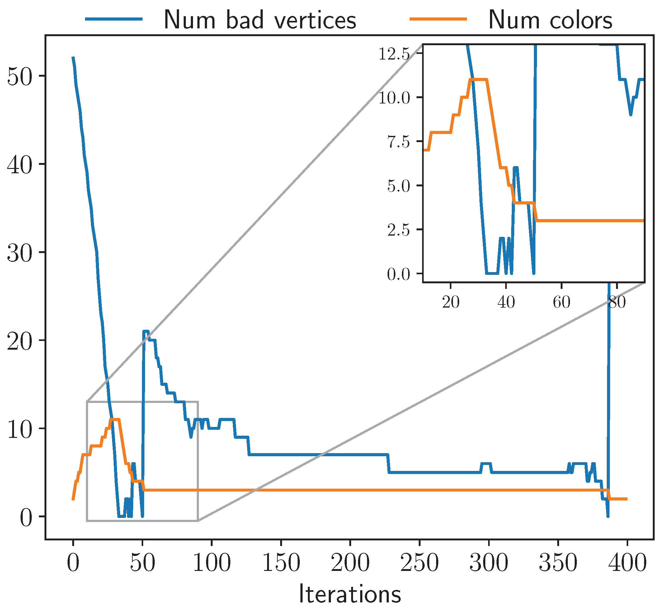
Figure 2.
Kendall’s correlation between base b and average convergence iterations across varying densities. Asterisks indicate statistical significance.
Figure 2.
Kendall’s correlation between base b and average convergence iterations across varying densities. Asterisks indicate statistical significance.
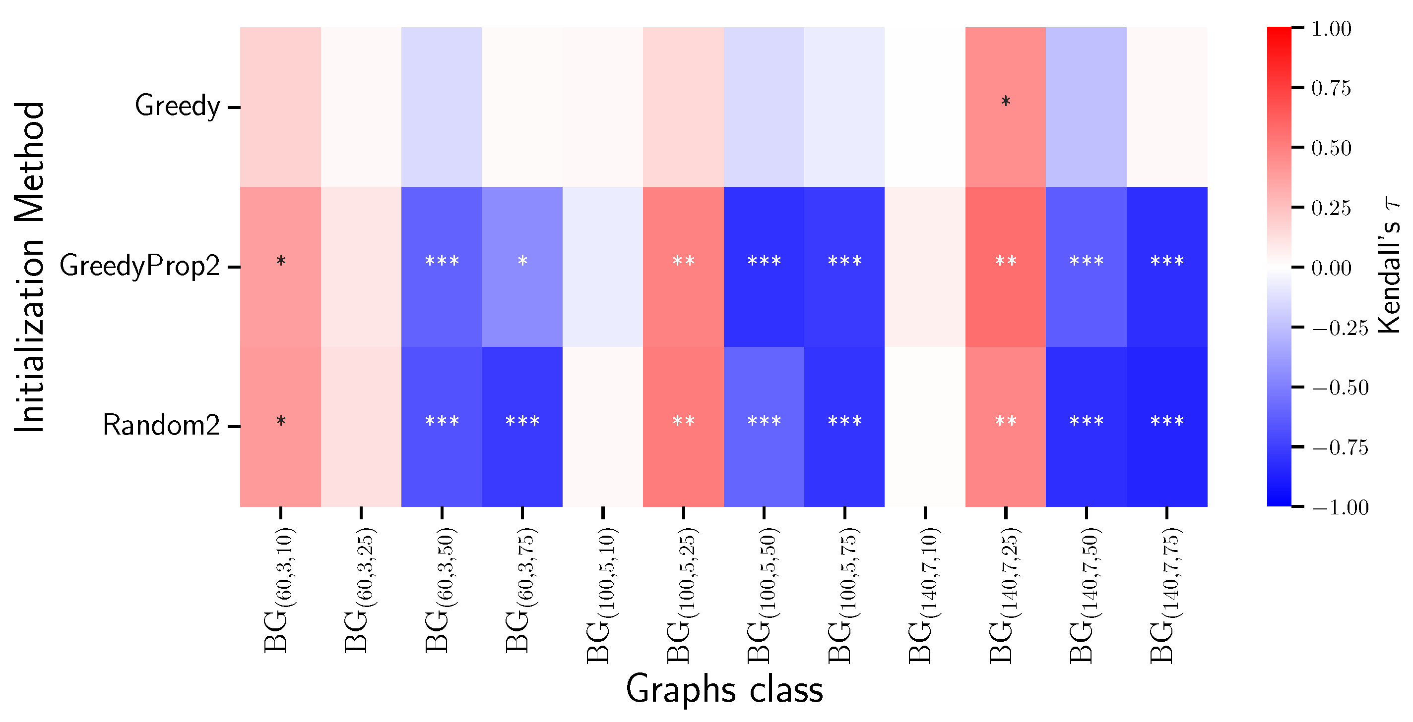
Figure 3.
Effect of base b on convergence for under Random2 initialization.
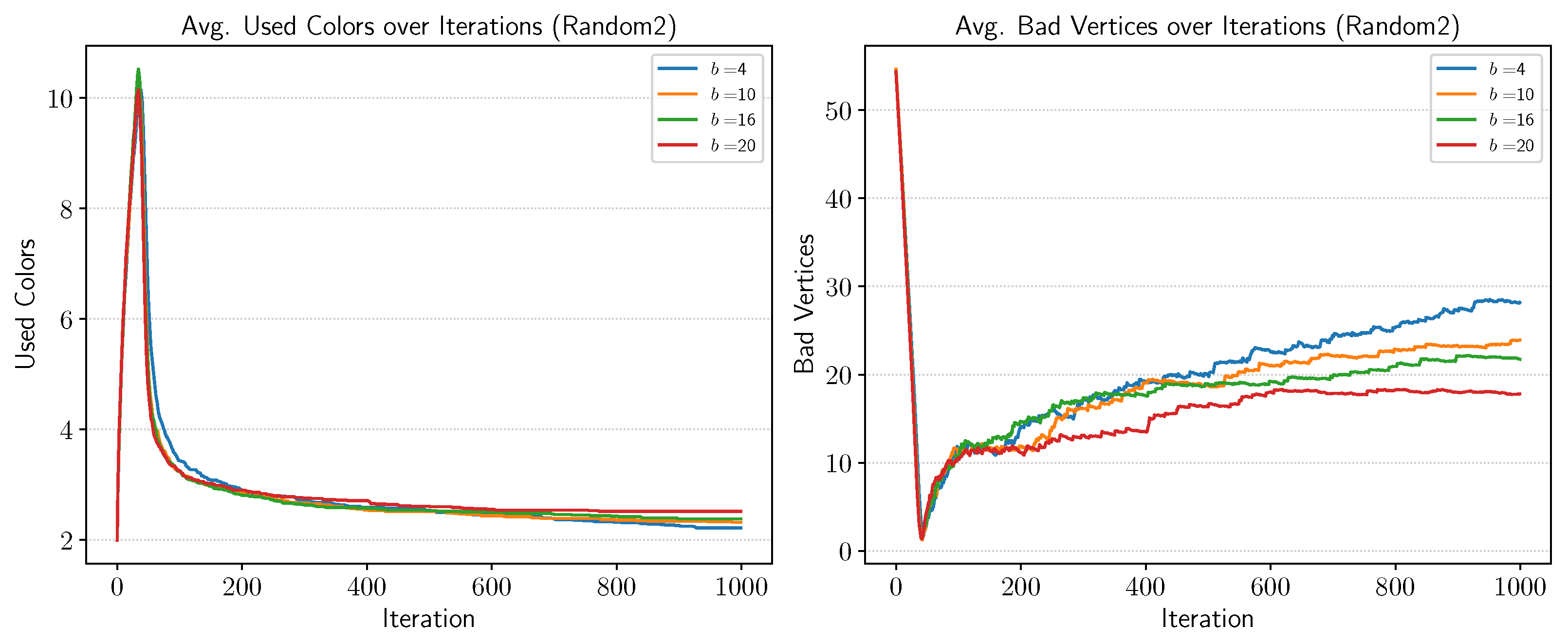
Figure 4.
Comparison of initialization strategies for at base .
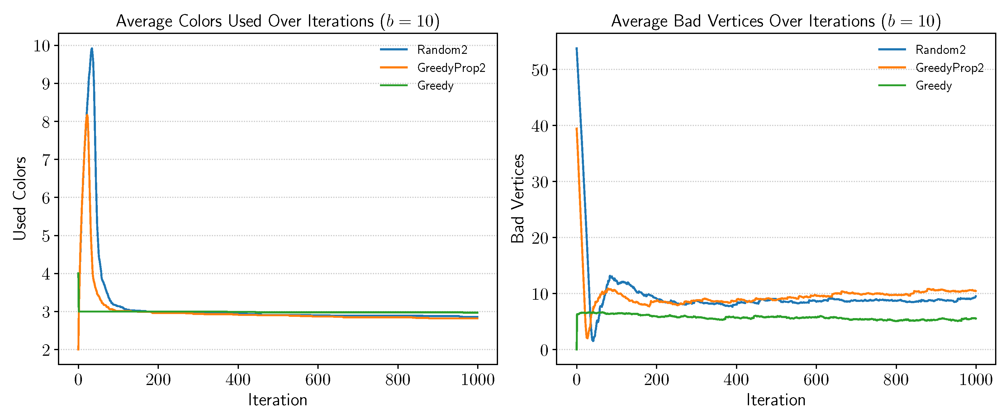
Figure 5.
Best value of k among all the bases, , using different initialization methods.
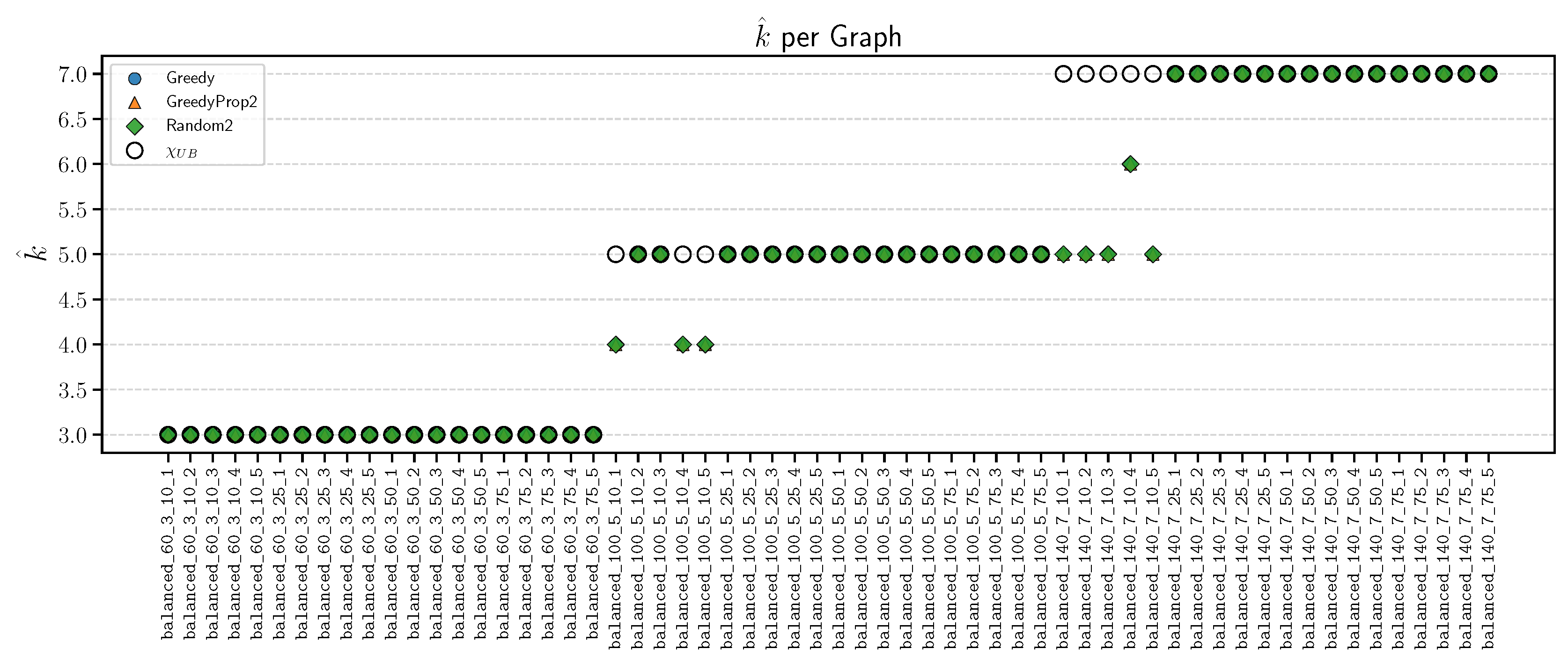
Figure 6.
Percent deviation of w.r.t. among all the bases using different initialization methods.
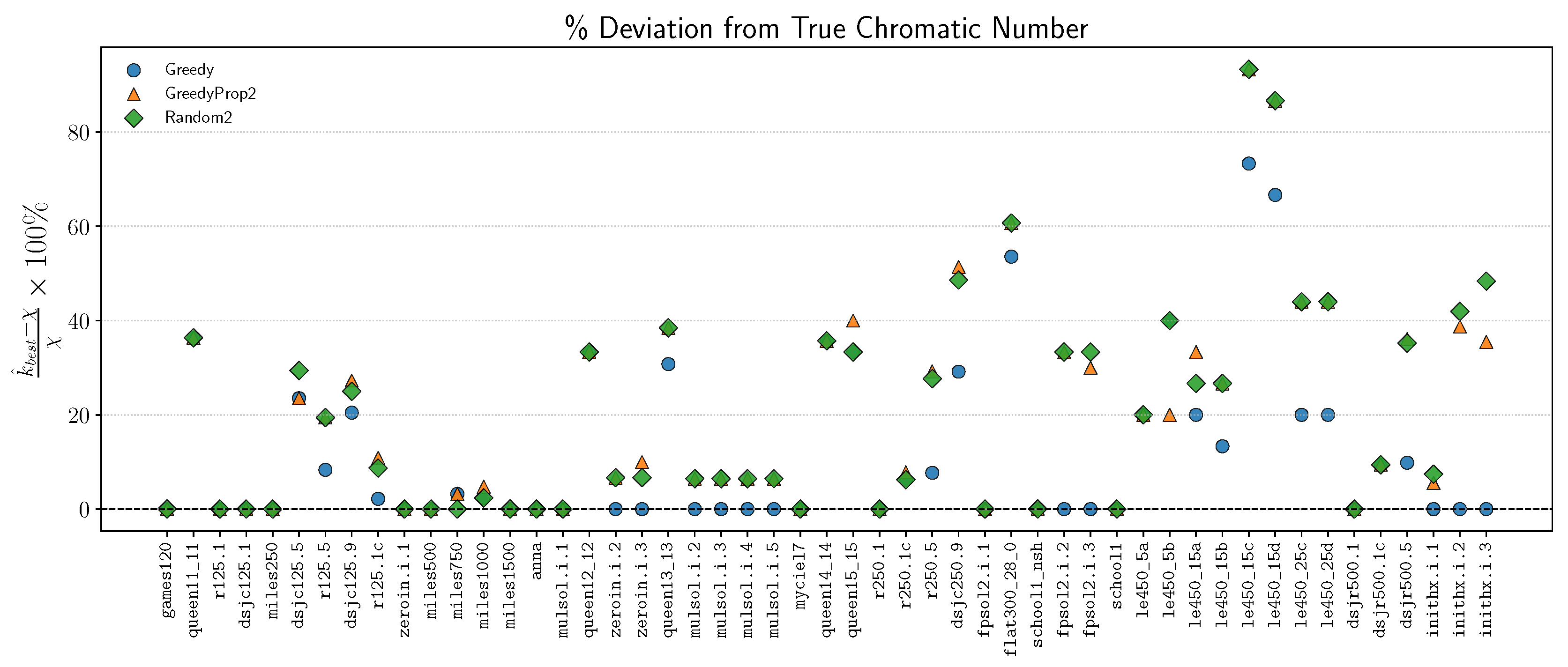

Table 1.
Table showing the found, , and mean iters. from different initial coloring methods at base = 10 for balanced k-partite graphs. The total number of tries was 100.
Table 1.
Table showing the found, , and mean iters. from different initial coloring methods at base = 10 for balanced k-partite graphs. The total number of tries was 100.
| Graph | N | (, mean iters.) | ||||
| Greedy | GreedyProp2 | RandomProp2 | ||||
| balanced_60_3_10_1 | 60 | 141 | 3 | (3, 100, 642.68) | (3, 100, 1302.94) | (3, 99, 1821.76) |
| balanced_60_3_10_2 | 60 | 113 | 3 | (3, 100, 106.49) | (3, 100, 465.34) | (3, 100, 569.14) |
| balanced_60_3_10_3 | 60 | 133 | 3 | (3, 74, 10190.38) | (3, 93, 7186.72) | (3, 94, 6029.05) |
| balanced_60_3_10_4 | 60 | 130 | 3 | (3, 100, 1530.08) | (3, 100, 1029.23) | (3, 100, 1176.21) |
| balanced_60_3_10_5 | 60 | 118 | 3 | (3, 100, 459.19) | (3, 100, 541.94) | (3, 100, 977.8) |
| balanced_60_3_25_1 | 60 | 286 | 3 | (3, 100, 138.41) | (3, 100, 244.05) | (3, 100, 310.88) |
| balanced_60_3_25_2 | 60 | 294 | 3 | (3, 100, 75.15) | (3, 100, 313.53) | (3, 100, 375.84) |
| balanced_60_3_25_3 | 60 | 307 | 3 | (3, 100, 780.74) | (3, 100, 253.35) | (3, 100, 347.57) |
| balanced_60_3_25_4 | 60 | 290 | 3 | (3, 100, 42.57) | (3, 100, 312.86) | (3, 100, 343.8) |
| balanced_60_3_25_5 | 60 | 305 | 3 | (3, 100, 416.05) | (3, 100, 380.13) | (3, 100, 366.63) |
| balanced_60_3_50_1 | 60 | 617 | 3 | (3, 100, 0.0) | (3, 100, 134.96) | (3, 100, 167.42) |
| balanced_60_3_50_2 | 60 | 620 | 3 | (3, 100, 12.45) | (3, 100, 139.09) | (3, 100, 161.89) |
| balanced_60_3_50_3 | 60 | 615 | 3 | (3, 100, 0.0) | (3, 100, 139.67) | (3, 100, 167.31) |
| balanced_60_3_50_4 | 60 | 607 | 3 | (3, 100, 101.06) | (3, 100, 140.56) | (3, 100, 155.89) |
| balanced_60_3_50_5 | 60 | 585 | 3 | (3, 100, 13.14) | (3, 100, 151.34) | (3, 100, 162.3) |
| balanced_60_3_75_1 | 60 | 922 | 3 | (3, 100, 18.46) | (3, 100, 123.56) | (3, 100, 144.42) |
| balanced_60_3_75_2 | 60 | 887 | 3 | (3, 100, 0.0) | (3, 100, 132.12) | (3, 100, 141.11) |
| balanced_60_3_75_3 | 60 | 873 | 3 | (3, 100, 0.0) | (3, 100, 127.72) | (3, 100, 148.82) |
| balanced_60_3_75_4 | 60 | 895 | 3 | (3, 100, 0.0) | (3, 100, 122.42) | (3, 100, 145.22) |
| balanced_60_3_75_5 | 60 | 886 | 3 | (3, 100, 0.0) | (3, 100, 125.22) | (3, 100, 145.73) |
| balanced_100_5_10_1 | 100 | 401 | 5 | (4, 87, 13128.01) | (4, 86, 16060.19) | (4, 81, 16753.02) |
| balanced_100_5_10_2 | 100 | 415 | 5 | (5, 100, 20.55) | (5, 100, 240.4) | (5, 100, 264.25) |
| balanced_100_5_10_3 | 100 | 437 | 5 | (5, 100, 55.58) | (5, 100, 306.05) | (5, 100, 321.21) |
| balanced_100_5_10_4 | 100 | 394 | 5 | (4, 78, 11475.01) | (4, 51, 20058.78) | (4, 55, 21395.64) |
| balanced_100_5_10_5 | 100 | 365 | 5 | (4, 100, 2782.52) | (4, 100, 4984.56) | (4, 100, 5133.19) |
| balanced_100_5_25_1 | 100 | 997 | 5 | (5, 100, 983.59) | (5, 100, 1649.32) | (5, 100, 1906.21) |
| balanced_100_5_25_2 | 100 | 955 | 5 | (5, 100, 5284.42) | (5, 100, 2634.18) | (5, 100, 2838.9) |
| balanced_100_5_25_3 | 100 | 1007 | 5 | (5, 100, 564.73) | (5, 100, 2511.9) | (5, 100, 2338.59) |
| balanced_100_5_25_4 | 100 | 1026 | 5 | (5, 100, 1221.94) | (5, 100, 1570.72) | (5, 100, 1549.94) |
| balanced_100_5_25_5 | 100 | 1047 | 5 | (5, 100, 2068.82) | (5, 100, 1785.53) | (5, 100, 1672.43) |
| balanced_100_5_50_1 | 100 | 2032 | 5 | (5, 100, 286.49) | (5, 100, 358.45) | (5, 100, 360.32) |
| balanced_100_5_50_2 | 100 | 2021 | 5 | (5, 100, 103.01) | (5, 100, 357.99) | (5, 100, 364.16) |
| balanced_100_5_50_3 | 100 | 2005 | 5 | (5, 100, 196.63) | (5, 100, 368.24) | (5, 100, 367.94) |
| balanced_100_5_50_4 | 100 | 2014 | 5 | (5, 100, 154.58) | (5, 100, 351.25) | (5, 100, 380.66) |
| balanced_100_5_50_5 | 100 | 2086 | 5 | (5, 100, 139.04) | (5, 100, 356.6) | (5, 100, 357.76) |
| balanced_100_5_75_1 | 100 | 2993 | 5 | (5, 100, 179.48) | (5, 100, 284.43) | (5, 100, 277.5) |
| balanced_100_5_75_2 | 100 | 2990 | 5 | (5, 100, 88.3) | (5, 100, 278.52) | (5, 100, 286.92) |
| balanced_100_5_75_3 | 100 | 3004 | 5 | (5, 100, 44.88) | (5, 100, 270.54) | (5, 100, 288.61) |
| balanced_100_5_75_4 | 100 | 2994 | 5 | (5, 100, 0.0) | (5, 100, 273.09) | (5, 100, 270.02) |
| balanced_100_5_75_5 | 100 | 3042 | 5 | (5, 100, 0.0) | (5, 100, 269.09) | (5, 100, 273.38) |
| balanced_140_7_10_1 | 140 | 826 | 7 | (5, 95, 18607.58) | (5, 94, 25152.38) | (5, 93, 24742.58) |
| balanced_140_7_10_2 | 140 | 837 | 7 | (5, 66, 34506.83) | (5, 67, 33209.18) | (5, 53, 27958.49) |
| balanced_140_7_10_3 | 140 | 836 | 7 | (5, 89, 25239.54) | (5, 83, 24031.25) | (5, 89, 29304.94) |
| balanced_140_7_10_4 | 140 | 880 | 7 | (6, 100, 411.99) | (6, 100, 706.27) | (6, 100, 732.43) |
| balanced_140_7_10_5 | 140 | 866 | 7 | (5, 21, 41444.86) | (5, 20, 34369.45) | (5, 27, 34863.89) |
| balanced_140_7_25_1 | 140 | 2079 | 7 | (7, 100, 8915.54) | (7, 100, 11801.03) | (7, 100, 10159.86) |
| balanced_140_7_25_2 | 140 | 2101 | 7 | (7, 100, 6355.96) | (7, 100, 10853.21) | (7, 100, 10400.25) |
| balanced_140_7_25_3 | 140 | 2099 | 7 | (7, 100, 8596.3) | (7, 100, 8723.64) | (7, 100, 8021.37) |
| balanced_140_7_25_4 | 140 | 2073 | 7 | (7, 100, 16328.22) | (7, 100, 11899.88) | (7, 100, 11190.06) |
| balanced_140_7_25_5 | 140 | 2081 | 7 | (7, 100, 11418.61) | (7, 99, 15249.36) | (7, 98, 15336.41) |
| balanced_140_7_50_1 | 140 | 4151 | 7 | (7, 100, 262.65) | (7, 100, 690.69) | (7, 100, 690.55) |
| balanced_140_7_50_2 | 140 | 4210 | 7 | (7, 100, 370.72) | (7, 100, 661.65) | (7, 100, 679.32) |
| balanced_140_7_50_3 | 140 | 4263 | 7 | (7, 100, 492.75) | (7, 100, 637.24) | (7, 100, 675.79) |
| balanced_140_7_50_4 | 140 | 4125 | 7 | (7, 100, 467.31) | (7, 100, 694.28) | (7, 100, 691.0) |
| balanced_140_7_50_5 | 140 | 4157 | 7 | (7, 100, 495.34) | (7, 100, 677.32) | (7, 100, 680.06) |
| balanced_140_7_75_1 | 140 | 6320 | 7 | (7, 100, 60.02) | (7, 100, 433.22) | (7, 100, 437.48) |
| balanced_140_7_75_2 | 140 | 6193 | 7 | (7, 100, 73.96) | (7, 100, 445.82) | (7, 100, 446.87) |
| balanced_140_7_75_3 | 140 | 6315 | 7 | (7, 100, 0.0) | (7, 100, 436.23) | (7, 100, 437.4) |
| balanced_140_7_75_4 | 140 | 6288 | 7 | (7, 100, 0.0) | (7, 100, 440.22) | (7, 100, 434.73) |
| balanced_140_7_75_5 | 140 | 6327 | 7 | (7, 100, 51.28) | (7, 100, 427.07) | (7, 100, 437.93) |
Table 2.
Table showing the found, , and mean iters. at different bases for Random2 initial coloring method for balanced k-partite graphs. The total number of tries was 100.
Table 2.
Table showing the found, , and mean iters. at different bases for Random2 initial coloring method for balanced k-partite graphs. The total number of tries was 100.
| Graph | N | (, mean iters.) | |||||
| 4 | 10 | 16 | 20 | ||||
| balanced_60_3_10_1 | 60 | 141 | 3 | (3, 100, 695.42) | (3, 99, 1821.76) | (3, 84, 2764.3) | (3, 89, 3865.74) |
| balanced_60_3_10_2 | 60 | 113 | 3 | (3, 100, 515.2) | (3, 100, 569.14) | (3, 100, 893.56) | (3, 100, 1006.98) |
| balanced_60_3_10_3 | 60 | 133 | 3 | (3, 99, 4693.02) | (3, 94, 6029.05) | (3, 71, 8626.0) | (3, 83, 8887.23) |
| balanced_60_3_10_4 | 60 | 130 | 3 | (3, 100, 943.75) | (3, 100, 1176.21) | (3, 99, 1645.39) | (3, 96, 2417.18) |
| balanced_60_3_10_5 | 60 | 118 | 3 | (3, 100, 642.64) | (3, 100, 977.8) | (3, 100, 1192.56) | (3, 100, 1638.29) |
| balanced_60_3_25_1 | 60 | 286 | 3 | (3, 100, 381.43) | (3, 100, 310.88) | (3, 100, 369.22) | (3, 100, 370.98) |
| balanced_60_3_25_2 | 60 | 294 | 3 | (3, 100, 395.92) | (3, 100, 375.84) | (3, 100, 465.47) | (3, 100, 377.13) |
| balanced_60_3_25_3 | 60 | 307 | 3 | (3, 100, 360.63) | (3, 100, 347.57) | (3, 100, 350.03) | (3, 100, 398.08) |
| balanced_60_3_25_4 | 60 | 290 | 3 | (3, 100, 422.08) | (3, 100, 343.8) | (3, 100, 403.84) | (3, 100, 520.77) |
| balanced_60_3_25_5 | 60 | 305 | 3 | (3, 100, 397.65) | (3, 100, 366.63) | (3, 100, 525.41) | (3, 100, 367.76) |
| balanced_60_3_50_1 | 60 | 617 | 3 | (3, 100, 195.69) | (3, 100, 167.42) | (3, 100, 159.6) | (3, 100, 153.43) |
| balanced_60_3_50_2 | 60 | 620 | 3 | (3, 100, 188.98) | (3, 100, 161.89) | (3, 100, 156.33) | (3, 100, 155.23) |
| balanced_60_3_50_3 | 60 | 615 | 3 | (3, 100, 203.25) | (3, 100, 167.31) | (3, 100, 161.82) | (3, 100, 160.19) |
| balanced_60_3_50_4 | 60 | 607 | 3 | (3, 100, 191.83) | (3, 100, 155.89) | (3, 100, 156.58) | (3, 100, 155.55) |
| balanced_60_3_50_5 | 60 | 585 | 3 | (3, 100, 205.22) | (3, 100, 162.3) | (3, 100, 165.02) | (3, 100, 162.7) |
| balanced_60_3_75_1 | 60 | 922 | 3 | (3, 100, 168.98) | (3, 100, 144.42) | (3, 100, 134.4) | (3, 100, 128.55) |
| balanced_60_3_75_2 | 60 | 887 | 3 | (3, 100, 170.32) | (3, 100, 141.11) | (3, 100, 134.14) | (3, 100, 139.94) |
| balanced_60_3_75_3 | 60 | 873 | 3 | (3, 100, 169.04) | (3, 100, 148.82) | (3, 100, 139.94) | (3, 100, 134.79) |
| balanced_60_3_75_4 | 60 | 895 | 3 | (3, 100, 172.41) | (3, 100, 145.22) | (3, 100, 139.99) | (3, 100, 133.7) |
| balanced_60_3_75_5 | 60 | 886 | 3 | (3, 100, 167.05) | (3, 100, 145.73) | (3, 100, 140.89) | (3, 100, 143.09) |
| balanced_100_5_10_1 | 100 | 401 | 5 | (4, 97, 13190.37) | (4, 81, 16753.02) | (4, 53, 16991.64) | (4, 46, 22098.61) |
| balanced_100_5_10_2 | 100 | 415 | 5 | (5, 100, 398.44) | (5, 100, 264.25) | (5, 100, 254.16) | (5, 100, 302.62) |
| balanced_100_5_10_3 | 100 | 437 | 5 | (5, 100, 511.94) | (5, 100, 321.21) | (5, 100, 344.07) | (5, 100, 341.93) |
| balanced_100_5_10_4 | 100 | 394 | 5 | (4, 74, 17104.27) | (4, 55, 21395.64) | (4, 36, 15245.31) | (4, 36, 18423.08) |
| balanced_100_5_10_5 | 100 | 365 | 5 | (4, 100, 6756.25) | (4, 100, 5133.19) | (4, 92, 7948.3) | (4, 90, 9283.31) |
| balanced_100_5_25_1 | 100 | 997 | 5 | (5, 100, 1912.59) | (5, 100, 1906.21) | (5, 100, 3172.81) | (5, 100, 2970.73) |
| balanced_100_5_25_2 | 100 | 955 | 5 | (5, 100, 2399.05) | (5, 100, 2838.9) | (5, 100, 4031.06) | (5, 98, 4129.43) |
| balanced_100_5_25_3 | 100 | 1007 | 5 | (5, 100, 2155.09) | (5, 100, 2338.59) | (5, 100, 3491.09) | (5, 100, 4366.11) |
| balanced_100_5_25_4 | 100 | 1026 | 5 | (5, 100, 1738.32) | (5, 100, 1549.94) | (5, 100, 2120.71) | (5, 99, 2405.43) |
| balanced_100_5_25_5 | 100 | 1047 | 5 | (5, 100, 1879.04) | (5, 100, 1672.43) | (5, 100, 2205.61) | (5, 99, 2809.86) |
| balanced_100_5_50_1 | 100 | 2032 | 5 | (5, 100, 494.76) | (5, 100, 360.32) | (5, 100, 353.94) | (5, 100, 363.79) |
| balanced_100_5_50_2 | 100 | 2021 | 5 | (5, 100, 486.64) | (5, 100, 364.16) | (5, 100, 356.96) | (5, 100, 362.47) |
| balanced_100_5_50_3 | 100 | 2005 | 5 | (5, 100, 500.43) | (5, 100, 367.94) | (5, 100, 355.03) | (5, 100, 342.84) |
| balanced_100_5_50_4 | 100 | 2014 | 5 | (5, 100, 496.93) | (5, 100, 380.66) | (5, 100, 363.29) | (5, 100, 368.81) |
| balanced_100_5_50_5 | 100 | 2086 | 5 | (5, 100, 468.94) | (5, 100, 357.76) | (5, 100, 352.61) | (5, 100, 343.38) |
| balanced_100_5_75_1 | 100 | 2993 | 5 | (5, 100, 364.13) | (5, 100, 277.5) | (5, 100, 265.89) | (5, 100, 258.95) |
| balanced_100_5_75_2 | 100 | 2990 | 5 | (5, 100, 360.49) | (5, 100, 286.92) | (5, 100, 265.55) | (5, 100, 268.35) |
| balanced_100_5_75_3 | 100 | 3004 | 5 | (5, 100, 366.07) | (5, 100, 288.61) | (5, 100, 268.0) | (5, 100, 266.7) |
| balanced_100_5_75_4 | 100 | 2994 | 5 | (5, 100, 355.45) | (5, 100, 270.02) | (5, 100, 270.02) | (5, 100, 251.35) |
| balanced_100_5_75_5 | 100 | 3042 | 5 | (5, 100, 371.88) | (5, 100, 273.38) | (5, 100, 258.92) | (5, 100, 257.87) |
| balanced_140_7_10_1 | 140 | 826 | 7 | (5, 18, 35862.94) | (5, 93, 24742.58) | (5, 64, 28914.0) | (5, 49, 35911.02) |
| balanced_140_7_10_2 | 140 | 837 | 7 | (5, 1, 57864.0) | (5, 53, 27958.49) | (5, 29, 35530.97) | (5, 14, 33685.79) |
| balanced_140_7_10_3 | 140 | 836 | 7 | (5, 13, 36733.54) | (5, 89, 29304.94) | (5, 55, 35117.38) | (5, 41, 27400.78) |
| balanced_140_7_10_4 | 140 | 880 | 7 | (6, 100, 1512.85) | (6, 100, 732.43) | (6, 100, 784.11) | (6, 100, 773.35) |
| balanced_140_7_10_5 | 140 | 866 | 7 | (5, 1, 16516.0) | (5, 27, 34863.89) | (5, 12, 46650.42) | (5, 3, 41211.67) |
| balanced_140_7_25_1 | 140 | 2079 | 7 | (7, 100, 11995.24) | (7, 100, 10159.86) | (7, 100, 18648.95) | (7, 93, 20292.3) |
| balanced_140_7_25_2 | 140 | 2101 | 7 | (7, 100, 10610.82) | (7, 100, 10400.25) | (7, 95, 17490.02) | (7, 89, 19993.64) |
| balanced_140_7_25_3 | 140 | 2099 | 7 | (7, 100, 12229.11) | (7, 100, 8021.37) | (7, 96, 15969.44) | (7, 91, 18847.48) |
| balanced_140_7_25_4 | 140 | 2073 | 7 | (7, 100, 18558.72) | (7, 100, 11190.06) | (7, 92, 19471.47) | (7, 81, 23240.46) |
| balanced_140_7_25_5 | 140 | 2081 | 7 | (7, 97, 21587.37) | (7, 98, 15336.41) | (7, 87, 24726.77) | (7, 75, 25699.41) |
| balanced_140_7_50_1 | 140 | 4151 | 7 | (7, 100, 1008.77) | (7, 100, 690.55) | (7, 100, 668.54) | (7, 100, 621.5) |
| balanced_140_7_50_2 | 140 | 4210 | 7 | (7, 100, 982.48) | (7, 100, 679.32) | (7, 100, 633.29) | (7, 100, 621.91) |
| balanced_140_7_50_3 | 140 | 4263 | 7 | (7, 100, 949.27) | (7, 100, 675.79) | (7, 100, 637.21) | (7, 100, 586.59) |
| balanced_140_7_50_4 | 140 | 4125 | 7 | (7, 100, 989.17) | (7, 100, 691.0) | (7, 100, 672.0) | (7, 100, 652.75) |
| balanced_140_7_50_5 | 140 | 4157 | 7 | (7, 100, 1004.81) | (7, 100, 680.06) | (7, 100, 641.17) | (7, 100, 648.6) |
| balanced_140_7_75_1 | 140 | 6320 | 7 | (7, 100, 615.39) | (7, 100, 437.48) | (7, 100, 414.44) | (7, 100, 401.85) |
| balanced_140_7_75_2 | 140 | 6193 | 7 | (7, 100, 632.38) | (7, 100, 446.87) | (7, 100, 412.05) | (7, 100, 402.7) |
| balanced_140_7_75_3 | 140 | 6315 | 7 | (7, 100, 610.55) | (7, 100, 437.4) | (7, 100, 414.22) | (7, 100, 393.11) |
| balanced_140_7_75_4 | 140 | 6288 | 7 | (7, 100, 619.77) | (7, 100, 434.73) | (7, 100, 411.04) | (7, 100, 395.9) |
| balanced_140_7_75_5 | 140 | 6327 | 7 | (7, 100, 631.73) | (7, 100, 437.93) | (7, 100, 396.85) | (7, 100, 397.37) |
Table 3.
Table showing the found, , and mean iters. from different initial coloring methods at base = 10 for DIMACS graphs. The total number of tries was 10.
Table 3.
Table showing the found, , and mean iters. from different initial coloring methods at base = 10 for DIMACS graphs. The total number of tries was 10.
| Graph | N | (, mean iters.) | ||||
| Greedy | GreedyProp2 | RandomProp2 | ||||
| queen10_10 | 100 | 1470 | 11 | (12, 10, 2424.0) | (12, 10, 4409.7) | (12, 10, 6195.8) |
| games120 | 120 | 638 | 9 | (9, 10, 0.0) | (9, 10, 130.4) | (9, 10, 134.4) |
| queen11_11 | 121 | 1980 | 11 | (13, 9, 20870.7) | (13, 9, 27059.1) | (13, 10, 32604.3) |
| r125.1 | (122, 125*) | 209 | 5 | (5, 10, 0.0) | (5, 10, 90.7) | (5, 10, 104.4) |
| dsjc125.1 | 125 | 736 | 5 | (5, 8, 34609.1) | (5, 8, 29797.5) | (5, 7, 20002.1) |
| dsjc125.5 | 125 | 3891 | 17 | (18, 1, 20353.0) | (19, 10, 7272.5) | (18, 1, 17936.0) |
| dsjc125.9 | 125 | 6961 | 44 | (48, 9, 17507.1) | (48, 8, 19232.4) | (47, 1, 42144.0) |
| miles250 | (125, 128*) | 387 | 8 | (8, 10, 0.0) | (8, 10, 182.7) | (8, 10, 248.2) |
| r125.1c | 125 | 7501 | 46 | (46, 10, 1130.9) | (46, 10, 7622.2) | (46, 10, 8777.6) |
| r125.5 | 125 | 3838 | 36 | (38, 2, 72.0) | (40, 10, 20087.7) | (40, 10, 21611.7) |
| zeroin.i.1 | (126, 211*) | 4100 | 49 | (49, 10, 0.0) | (49, 4, 35532.0) | (49, 7, 24083.0) |
| miles1000 | 128 | 3216 | 42 | (42, 5, 11994.6) | (42, 3, 38704.3) | (42, 6, 20584.8) |
| miles1500 | 128 | 5198 | 73 | (73, 10, 0.0) | (73, 10, 2960.7) | (73, 10, 2937.4) |
| miles500 | 128 | 1170 | 20 | (20, 10, 0.0) | (20, 10, 739.0) | (20, 10, 708.7) |
| miles750 | 128 | 2113 | 31 | (31, 8, 6198.0) | (31, 9, 20833.4) | (31, 8, 24205.4) |
| anna | 138 | 493 | 11 | (11, 10, 0.0) | (11, 10, 393.7) | (11, 10, 386.9) |
| mulsol.i.1 | (138, 197*) | 3925 | 49 | (49, 10, 0.0) | (49, 10, 10602.4) | (49, 10, 8138.3) |
| queen12_12 | 144 | 2596 | 12 | (14, 2, 61455.0) | (14, 2, 37436.5) | (14, 2, 31584.0) |
| zeroin.i.2 | (157, 211*) | 3541 | 30 | (30, 10, 0.0) | (31, 1, 76718.0) | (32, 3, 37033.3) |
| zeroin.i.3 | (157, 206*) | 3540 | 30 | (30, 10, 0.0) | (32, 3, 28664.7) | (31, 1, 28682.0) |
| queen13_13 | 169 | 3328 | 13 | (16, 10, 3766.9) | (16, 10, 3931.6) | (16, 10, 2236.1) |
| mulsol.i.2 | (173, 188*) | 3885 | 31 | (31, 10, 0.0) | (32, 2, 21774.5) | (33, 6, 20340.2) |
| mulsol.i.3 | (174, 184*) | 3916 | 31 | (31, 10, 0.0) | (31, 1, 66168.0) | (32, 2, 53135.5) |
| mulsol.i.4 | (175, 185*) | 3946 | 31 | (31, 10, 0.0) | (33, 7, 36817.3) | (32, 2, 71797.5) |
| mulsol.i.5 | (176, 186*) | 3973 | 31 | (31, 10, 0.0) | (32, 2, 46180.0) | (31, 1, 80600.0) |
| myciel7 | 191 | 2360 | 8 | (8, 10, 0.0) | (8, 10, 444.9) | (8, 10, 838.4) |
| queen14_14 | 196 | 4186 | 14 | (17, 10, 16586.2) | (17, 10, 6326.1) | (17, 10, 12055.2) |
| queen15_15 | 225 | 5180 | 15 | (18, 6, 31860.2) | (18, 8, 42906.9) | (18, 5, 46113.6) |
| dsjc250.9 | 250 | 27897 | 72 | (81, 1, 85070.0) | (82, 1, 10028.0) | (81, 1, 69051.0) |
| r250.1 | 250 | 867 | 8 | (8, 10, 0.0) | (8, 10, 261.9) | (8, 10, 269.6) |
| r250.1c | 250 | 30227 | 64 | (64, 9, 36834.7) | (64, 9, 30456.6) | (64, 7, 34651.6) |
| r250.5 | 250 | 14849 | 65 | (70, 10, 0.0) | (76, 1, 121885.0) | (77, 5, 68487.4) |
| fpsol2.i.1 | (269, 496*) | 11654 | 65 | (65, 10, 0.0) | (65, 7, 77886.9) | (65, 9, 88497.9) |
| flat300_28_0 | 300 | 21695 | 28 | (36, 1, 135010.0) | (36, 2, 93484.0) | (36, 6, 102437.5) |
| school1_nsh | 352 | 14612 | 14 | (14, 9, 21266.3) | (14, 9, 8520.3) | (14, 8, 14151.0) |
| fpsol2.i.2 | (363, 451*) | 8691 | 30 | (30, 10, 0.0) | (38, 2, 83531.0) | (38, 1, 90906.0) |
| fpsol2.i.3 | (363, 425*) | 8688 | 30 | (30, 10, 0.0) | (38, 2, 102963.5) | (36, 1, 141087.0) |
| school1 | 385 | 19095 | 14 | (14, 9, 23410.7) | (14, 9, 6986.8) | (14, 10, 11152.2) |
| le450_15a | 450 | 8168 | 15 | (16, 1, 173285.0) | (17, 10, 6486.9) | (17, 10, 6299.5) |
| le450_15b | 450 | 8169 | 15 | (17, 10, 9.7) | (17, 10, 7481.9) | (16, 2, 136735.0) |
| le450_15c | 450 | 16680 | 15 | (16, 1, 187434.0) | (17, 9, 154051.8) | (16, 1, 123032.0) |
| le450_15d | 450 | 16750 | 15 | (17, 7, 139141.7) | (17, 10, 134227.2) | (16, 1, 175603.0) |
| le450_25c | 450 | 17343 | 25 | (29, 6, 101.0) | (29, 1, 185791.0) | (30, 10, 87136.5) |
| le450_25d | 450 | 17425 | 25 | (29, 6, 178.5) | (30, 10, 78094.9) | (30, 9, 41700.2) |
| le450_5a | 450 | 5714 | 5 | (6, 3, 96363.3) | (6, 5, 28477.6) | (6, 6, 79516.3) |
| le450_5b | 450 | 5734 | 5 | (6, 4, 144962.2) | (6, 4, 72683.5) | (6, 5, 89260.0) |
| dsjr500.1 | 500 | 3555 | 12 | (12, 10, 127.6) | (12, 10, 1596.9) | (12, 10, 1672.4) |
| dsjr500.1c | 500 | 121275 | 85 | (86, 5, 123670.8) | (86, 2, 192601.5) | (87, 6, 145665.0) |
| dsjr500.5 | 500 | 58862 | 122 | (133, 3, 11.3) | (149, 1, 7558.0) | (150, 3, 127779.3) |
| inithx.i.1 | (519, 864*) | 18707 | 54 | (54, 10, 0.0) | (56, 1, 216367.0) | (55, 1, 201835.0) |
| inithx.i.2 | (558, 645*) | 13979 | 31 | (31, 10, 0.0) | (40, 1, 217881.0) | (43, 1, 218428.0) |
| inithx.i.3 | (559, 621*) | 13969 | 31 | (31, 10, 0.0) | (42, 1, 154076.0) | (43, 1, 25165.0) |
Table 4.
Table showing the found, , and mean iters. at different bases for Random2 initial coloring method for DIMACS graphs. The total number of tries was 10.
Table 4.
Table showing the found, , and mean iters. at different bases for Random2 initial coloring method for DIMACS graphs. The total number of tries was 10.
| Graph | N | (, mean iters.) | |||||
| 4 | 10 | 16 | 20 | ||||
| games120 | 120 | 638 | 9 | (9, 10, 177.3) | (9, 10, 134.4) | (9, 10, 126.9) | (9, 10, 128.1) |
| queen11_11 | 121 | 1980 | 11 | (15, 10, 2769.0) | (13, 10, 32604.3) | (13, 10, 4902.1) | (13, 10, 2155.5) |
| r125.1 | (122, 125*) | 209 | 5 | (5, 10, 121.9) | (5, 10, 104.4) | (5, 10, 104.2) | (5, 10, 97.0) |
| dsjc125.1 | 125 | 736 | 5 | (5, 1, 33786.0) | (5, 7, 20002.1) | (5, 6, 18344.8) | (5, 1, 10833.0) |
| miles250 | (125, 128*) | 387 | 8 | (8, 10, 317.3) | (8, 10, 248.2) | (8, 10, 243.8) | (8, 10, 148.8) |
| r125.1c | 125 | 7501 | 46 | (50, 1, 59577.0) | (46, 10, 8777.6) | (46, 10, 9069.3) | (46, 9, 15232.7) |
| dsjc125.9 | 125 | 6961 | 44 | (55, 1, 6142.0) | (47, 1, 42144.0) | (45, 1, 4447.0) | (45, 2, 28926.0) |
| dsjc125.5 | 125 | 3891 | 17 | (22, 10, 24273.1) | (18, 1, 17936.0) | (18, 10, 16079.5) | (18, 10, 15916.4) |
| r125.5 | 125 | 3838 | 36 | (43, 6, 19662.5) | (40, 10, 21611.7) | (39, 10, 18904.4) | (38, 2, 31847.5) |
| zeroin.i.1 | (126, 211*) | 4100 | 49 | (49, 10, 18571.4) | (49, 7, 24083.0) | (49, 2, 38714.5) | (49, 1, 14981.0) |
| miles500 | 128 | 1170 | 20 | (20, 10, 4683.0) | (20, 10, 708.7) | (20, 10, 582.5) | (20, 10, 648.7) |
| miles1500 | 128 | 5198 | 73 | (73, 3, 27536.7) | (73, 10, 2937.4) | (73, 10, 2347.4) | (73, 10, 2365.5) |
| miles750 | 128 | 2113 | 31 | (31, 1, 58027.0) | (31, 8, 24205.4) | (31, 10, 9100.0) | (31, 10, 6223.3) |
| miles1000 | 128 | 3216 | 42 | (43, 1, 16999.0) | (42, 6, 20584.8) | (42, 8, 11433.0) | (42, 10, 18577.8) |
| mulsol.i.1 | (138, 197*) | 3925 | 49 | (49, 10, 3733.0) | (49, 10, 8138.3) | (49, 10, 11425.8) | (49, 10, 5581.1) |
| anna | 138 | 493 | 11 | (11, 10, 372.8) | (11, 10, 386.9) | (11, 10, 433.7) | (11, 10, 4241.2) |
| queen12_12 | 144 | 2596 | 12 | (16, 10, 23088.2) | (14, 2, 31584.0) | (14, 10, 10706.6) | (14, 10, 4711.0) |
| zeroin.i.2 | (157, 211*) | 3541 | 30 | (30, 3, 47465.0) | (32, 3, 37033.3) | (32, 1, 27708.0) | (32, 1, 40091.0) |
| zeroin.i.3 | (157, 206*) | 3540 | 30 | (30, 4, 45605.8) | (31, 1, 28682.0) | (32, 1, 41272.0) | (32, 2, 55011.0) |
| queen13_13 | 169 | 3328 | 13 | (18, 10, 2047.7) | (16, 10, 2236.1) | (15, 8, 21428.2) | (15, 10, 7008.4) |
| mulsol.i.2 | (173, 188*) | 3885 | 31 | (31, 4, 27328.5) | (33, 6, 20340.2) | (33, 3, 37431.0) | (33, 6, 34503.5) |
| mulsol.i.3 | (174, 184*) | 3916 | 31 | (31, 4, 60165.0) | (32, 2, 53135.5) | (33, 4, 31618.5) | (33, 4, 60413.5) |
| mulsol.i.4 | (175, 185*) | 3946 | 31 | (31, 5, 40779.6) | (32, 2, 71797.5) | (32, 1, 20705.0) | (33, 4, 47436.8) |
| mulsol.i.5 | (176, 186*) | 3973 | 31 | (31, 2, 21881.0) | (31, 1, 80600.0) | (32, 2, 41175.0) | (33, 4, 61435.2) |
| myciel7 | 191 | 2360 | 8 | (8, 10, 490.2) | (8, 10, 838.4) | (8, 9, 768.7) | (8, 10, 4736.4) |
| queen14_14 | 196 | 4186 | 14 | (19, 10, 17020.5) | (17, 10, 12055.2) | (16, 1, 13392.0) | (16, 6, 35802.7) |
| queen15_15 | 225 | 5180 | 15 | (20, 1, 112258.0) | (18, 5, 46113.6) | (18, 10, 3611.6) | (17, 2, 59238.0) |
| r250.1c | 250 | 30227 | 64 | (68, 1, 39166.0) | (64, 7, 34651.6) | (64, 7, 47749.0) | (64, 6, 48614.7) |
| r250.1 | 250 | 867 | 8 | (8, 10, 382.2) | (8, 10, 269.6) | (8, 10, 261.3) | (8, 10, 337.1) |
| dsjc250.9 | 250 | 27897 | 72 | (107, 1, 47221.0) | (81, 1, 69051.0) | (79, 3, 43635.7) | (78, 6, 79146.7) |
| r250.5 | 250 | 14849 | 65 | (83, 2, 88465.5) | (77, 5, 68487.4) | (74, 2, 65300.5) | (74, 5, 48315.4) |
| fpsol2.i.1 | (269, 496*) | 11654 | 65 | (65, 10, 31441.9) | (65, 9, 88497.9) | (65, 5, 105803.4) | (65, 2, 102137.0) |
| flat300_28_0 | 300 | 21695 | 28 | (45, 4, 50999.5) | (36, 6, 102437.5) | (33, 1, 143072.0) | (32, 1, 88643.0) |
| school1_nsh | 352 | 14612 | 14 | (14, 10, 10003.8) | (14, 8, 14151.0) | (14, 5, 63549.0) | (14, 6, 27482.8) |
| fpsol2.i.3 | (363, 425*) | 8688 | 30 | (35, 2, 119802.0) | (36, 1, 141087.0) | (39, 1, 98128.0) | (40, 1, 162869.0) |
| fpsol2.i.2 | (363, 451*) | 8691 | 30 | (34, 2, 109884.0) | (38, 1, 90906.0) | (37, 1, 145146.0) | (40, 1, 66835.0) |
| school1 | 385 | 19095 | 14 | (14, 10, 7080.2) | (14, 10, 11152.2) | (14, 9, 17417.0) | (14, 10, 11591.4) |
| le450_5b | 450 | 5734 | 5 | (6, 10, 17455.8) | (6, 5, 89260.0) | (7, 10, 19146.4) | (7, 10, 52126.6) |
| le450_5a | 450 | 5714 | 5 | (5, 1, 169416.0) | (6, 6, 79516.3) | (6, 1, 137162.0) | (6, 4, 100053.0) |
| le450_15d | 450 | 16750 | 15 | (28, 1, 23854.0) | (16, 1, 175603.0) | (19, 1, 220765.0) | (20, 1, 194484.0) |
| le450_25c | 450 | 17343 | 25 | (36, 2, 151978.0) | (30, 10, 87136.5) | (28, 10, 77927.4) | (27, 4, 100118.0) |
| le450_25d | 450 | 17425 | 25 | (36, 3, 37371.0) | (30, 9, 41700.2) | (28, 10, 63732.8) | (27, 8, 139768.8) |
| le450_15c | 450 | 16680 | 15 | (29, 10, 24378.9) | (16, 1, 123032.0) | (20, 3, 180997.3) | (20, 1, 187445.0) |
| le450_15b | 450 | 8169 | 15 | (19, 1, 150060.0) | (16, 2, 136735.0) | (16, 10, 16153.4) | (15, 2, 112835.5) |
| le450_15a | 450 | 8168 | 15 | (19, 2, 95430.5) | (17, 10, 6299.5) | (16, 10, 18193.5) | (15, 1, 121410.0) |
| dsjr500.1c | 500 | 121275 | 85 | (93, 1, 84314.0) | (87, 6, 145665.0) | (86, 2, 185044.5) | (86, 1, 202039.0) |
| dsjr500.1 | 500 | 3555 | 12 | (12, 10, 5808.9) | (12, 10, 1672.4) | (12, 10, 1355.3) | (12, 10, 1343.8) |
| dsjr500.5 | 500 | 58862 | 122 | (165, 1, 244534.0) | (150, 3, 127779.3) | (145, 4, 121450.5) | (143, 1, 216451.0) |
| inithx.i.1 | (519, 864*) | 18707 | 54 | (54, 8, 184365.0) | (55, 1, 201835.0) | (58, 2, 188375.0) | (56, 1, 174260.0) |
| inithx.i.2 | (558, 645*) | 13979 | 31 | (38, 1, 181649.0) | (43, 1, 218428.0) | (44, 1, 208224.0) | (44, 1, 113023.0) |
| inithx.i.3 | (559, 621*) | 13969 | 31 | (38, 1, 153621.0) | (43, 1, 25165.0) | (43, 2, 138566.5) | (46, 2, 114019.0) |
Disclaimer/Publisher’s Note: The statements, opinions and data contained in all publications are solely those of the individual author(s) and contributor(s) and not of MDPI and/or the editor(s). MDPI and/or the editor(s) disclaim responsibility for any injury to people or property resulting from any ideas, methods, instructions or products referred to in the content. |
© 2024 by the authors. Licensee MDPI, Basel, Switzerland. This article is an open access article distributed under the terms and conditions of the Creative Commons Attribution (CC BY) license (https://creativecommons.org/licenses/by/4.0/).
Copyright: This open access article is published under a Creative Commons CC BY 4.0 license, which permit the free download, distribution, and reuse, provided that the author and preprint are cited in any reuse.


