
Submitted:
20 August 2025
Posted:
21 August 2025
You are already at the latest version
Abstract
Vegetated intertidal ecosystems, such as seagrass meadows, salt marshes, and macroalgal beds, are vital for biodiversity, coastal protection, and climate regulation; however, they remain highly vulnerable to anthropogenic and climate-induced stressors. This study aims to assess interannual changes in intertidal vegetation cover along the Portuguese mainland coast from 2015 to 2024 using Sentinel-2 satellite imagery calibrated with high-resolution multispectral UAV data, to determine the most accurate index for map-ping intertidal vegetation. Among the 16 indices tested, the Atmospherically Resilient Vegetation Index (ARVI) showed the highest predictive performance. An ARVI threshold value of 0.19 was established to delineate vegetated areas. Applying this threshold to time-series data revealed considerable spatial and temporal variability in vegetation cover, with estuarine systems such as the Ria de Aveiro and the Ria Formosa showing the great-est extents and fluctuations. At the national level, vegetation cover reflects both regional environmental dynamics and data acquisition limitations. Despite limitations related to satellite image resolution and single-site validation, the results demonstrate the feasibility and utility of combining UAV data and satellite indices for long-term, large-scale monitoring of intertidal vegetation.
Keywords:
Sentinel-2
; Intertidal
; Vegetation Index
; monitoring
; UAV
1. Introduction
Recent advances in remote sensing technologies have significantly improved our understanding of intertidal and wetland ecosystems [1]. Several studies have focused on monitoring, mapping and assessing intertidal seagrass meadows using high-resolution satellite imagery, especially from Sentinel-2 satellites, and drone technologies [2]. These tools have provided invaluable information on the phenology, distribution and ecological status of these vital coastal ecosystems.
Vegetated coastal ecosystems, such as saltmarshes, seagrass meadows and macroalgae, are vital for biodiversity, coastal protection, and climate regulation [3]. Despite occupying only a narrow strip of the global coastline, these ecosystems play an important role in carbon sequestration, sediment stabilisation, and nutrient cycling [4]. These ecosystems include the most productive marine habitats and provide crucial ecosystem services, acting as carbon sinks and barriers to erosion and sea level rise. However, in recent decades, up to 50% of their global extent has been lost due to land-use change and climate stressors such as marine heatwaves and accelerated sea level rise [4,5,6]. Monitoring the spatial and temporal dynamics of intertidal ecosystems is therefore essential for both conservation and adaptive coastal management.
Remote sensing (RS) has become an indispensable tool for monitoring intertidal vegetation at multiple spatial and temporal scales. At the local scale, unoccupied aerial vehicles (UAVs) equipped with multispectral sensors provide very high-resolution (centimetre-scale) imagery, which is particularly effective for field verification of satellite data [7,8]. At the regional and national scales, open-access satellite data from the Sentinel-2 mission, operated within the framework of the European Space Agency’s Copernicus Program, enable systematic monitoring of coastal ecosystems. Sentinel-2 imagery offers a spatial resolution of 10 m and a revisit frequency of five days [9,10].
Open-access Earth observation data have enabled applications in long-term monitoring programs, including those implemented in data-scarce or resource-limited contexts [9,11]. This makes satellite remote sensing a viable and cost-effective option for continuous monitoring of intertidal habitats over large geographic areas. However, several limitations remain when applying remote sensing to intertidal environments. Image quality is often limited by cloud cover and tidal variability, factors that can reduce detection accuracy [9,10]. Furthermore, given the spatial resolution of open-access satellite imagery (10 m or more for Sentinel-2 data) and the spatial variability of intertidal habitats, many intertidal pixels are prone to be of mixed nature, comprising a combination of vegetation, rocks, sediment, and water. This can distort the spectral signature for many small areas, leading to an underestimation of vegetation extents, especially in smaller or fragmented patches [8,12].
Despite these challenges, recent advances in satellite data processing and classification methods have improved the reliability of vegetation detection. This is the case in the research by Rowe Davies et al. [10], where they employed a neural network model (ICE CREAMS v1.0) with Sentinel-2 time-series data to track interannual changes in Zostera noltei meadows in Western Europe. Similarly, Mora-Soto et al. [11] developed a global map of intertidal giant kelp and green kelp forests based on Sentinel-2 data and threshold-based spectral indices. These applications highlight the growing potential of publicly available satellite imagery for long-term monitoring and conservation of vegetated coastal habitats, as well as adaptation to statistical models that enable monitoring or projections of these ecosystems.
Vegetation indices (VIs) derived from remote sensing surveys of coastal ecosystems have proven effective in mapping vegetation density at different scales, by detecting vegetation characteristics from multispectral images. The Normalised Difference Vegetation Index (NDVI), derived from red and near-infrared (NIR) reflectance, is one of the most widely used indices for assessing chlorophyll activity and estimating vegetation cover and biomass [8,9,11]. Although originally developed for terrestrial vegetation, NDVI and its derivatives have been successfully applied to monitoring intertidal seagrass beds and macroalgae [13].
A range of alternative VIs have been explored to address the limitations of NDVI in aquatic or mixed environments. This is the case with indicators such as Atmospherically Resistant Vegetation Index (ARVI), Soil-Adjusted Vegetation Index (SAVI), and Normalized Difference Water Index (NDWI), which have demonstrated improved performance in areas with high reflectance variability due to ground brightness or water interference [9]. Furthermore, spectral combinations, including red-edge bands and Short-Wave Infrared (SWIR), have shown great potential for capturing submerged or periodically flooded vegetation covers [11,12]. The Normalized Difference Moisture Index (NDMI), which strongly correlates with vegetation moisture content, is particularly valuable in coastal wetlands and estuarine environments, where hydrological variation plays a key role in vegetation dynamics [14].
More advanced methods, such as Tassel Transformation (TCT) [15] which transforms spectral data into brightness, greenness, and wetness components, are useful for identifying phenological stages and monitoring vegetation health over time. Similarly, Change Vector Analysis (CVA) [16], which assesses both the intensity and direction of spectral change, allows the detection of subtle land cover transitions or sudden disturbances, such as droughts or floods. These methods have proven useful for monitoring dynamic coastal habitats, and their responses to environmental stressors have expanded the capabilities of remote sensing.
Research such as that by Suir et al., [17] further demonstrated the utility of combining hyperspectral and LiDAR derived vegetation metrics to monitor temporal trends in coastal vegetation, including its response to extreme weather events, offering a more detailed and integrated understanding of ecosystem structure and function.
Other studies have applied harmonic regression to Landsat derived VI time series to extract phenological characteristics of Spartina alterniflora along the Guangxi coast [18]. Their results demonstrate the robustness of vegetation index when integrated with machine learning and ecological modelling for wetland management. Similarly, in another coastal ecosystem, Jia et al. [19] introduced the Mangrove Forest Index (MFI), specifically designed to identify submerged mangrove forests using single tide Sentinel-2 imagery.
Through analysis of satellite image time series, these indices and transformations support the assessment of interannual and seasonal trends in intertidal vegetation. This provides information on ecosystem health and its vulnerability to disturbances such as sea level rise, storms, and invasive species [6,10].
The aim of this study was to analyse interannual changes in intertidal vegetation cover along the coast of Portugal for the past decade (i.e., since Sentinel-2 data became available). The integration of Sentinel-2 imagery, drone based multispectral observations, and a wide range of vegetation indices is proposed to improve the monitoring of intertidal habitats. Therefore, 10-m resolution satellite remote sensing data are calibrated with high-resolution UAV data to assess (i) the distribution of coastal intertidal vegetation and (ii) its variation from 2015 to 2024. Several vegetation indices derived from satellite images are tested, assessing their ability to represent the true intertidal vegetation cover, obtained through very-high-resolution and in-situ surveys for a test area. The applicability and limitations of the methodology and the use of these satellite data are discussed.
2. Materials and Methods
2.1. Procedure
Data processing involved several sequential steps designed to estimate and map intertidal vegetation cover using satellite data and the relationship between vegetation indices and vegetation cover, validated for an area with high resolution and in-situ information (Figure 1):
- Very-high-resolution multispectral UAV imagery from the Viana de Castelo area in northern Portugal was classified using supervised machine learning techniques, to obtain reference maps of vegetation cover in intertidal zones.
- Statistical regression models were developed to quantify the relationship between UAV-derived vegetation cover and Sentinel-2 vegetation index values.
- The best-performing vegetation index was used for the estimation of vegetation cover. A model threshold value was established to determine which satellite pixels are vegetation
- The selected VI and respective threshold were applied to the entire satellite time series of multispectral bands of the Sentinel-2 mosaics to assess the spatial extent and temporal variability of intertidal vegetation during the study period.
2.2. Satellite Image Selection and Processing
Sentinel-2 images (Level 2A) were obtained from the Copernicus Explore portal [20]. Data are provided in approximately 100×100 km tiles, 9 of which cover the Portuguese coastline (Figure 2). Image dates were selected applying the following criteria: negligible cloud cover, capture during spring/summer season, to avoid vegetation differences due to seasonality; and, image capture date and time corresponding to the lowest tide possible. To ensure good image quality, all satellite image tiles with up to 10% cloud cover were visually checked, selecting the image with the lowest tide that showed no significant cloud cover over the intertidal areas.
Tidal elevations were obtained from gridded sets of tidal harmonic constants (eight primary, two long period and three non-linear components) from the TPXO9-atlas with a 1/30 degrees’ resolution, using the Tidal Model Driver (TMD) tool [21]. The selected model assimilates various altimetric products as well as other coastal data sets, providing accurate results for complex topographic areas and in shallow waters. The astronomical tide was extracted for each satellite image tile (considering the coordinates in the centre of the respective coastal stretch), for all dates between May and August, for the years 2015 to 2024, for the time of satellite passage 11:21h (UTC).
For each of the selected tiles, the Sentinel-2 Blue, Green, Red and NIR bands (central wavelengths 490 nm, 560 nm, 665 nm and 842nm, respectively; 10-m resolution) were downloaded. The tiles, which are partially overlapping (Figure 2), were merged into a single mosaic per year, averaging the band values in the overlapping pixels (to avoid duplicate pixels for a single year).
The mosaic was then clipped to the intertidal zone. Given the tides in Portugal, which generally range between 2 m above and 2 m below Mean Sea Level (MSL), the study area was delimited to the coastal stretch with elevation up to 2 m above MSL, on the land side, and by 2 m below MSL on the ocean side. Elevations were obtained from the Digital Terrain Model (DTM) of a national LIDAR survey carried out in 2011 (data provided by the Portuguese Direção Geral do Território (DGT) [22], which has a spatial resolution of 2 meters and covers the whole continental Portuguese coast. The resulting intertidal area was further visually checked and manually adapted to eliminate non-natural habitats (like forests, agriculture fields and parks) from the study area.
Analyses were done for the whole coastline and per region, considering geomorphological consistency and coastal configuration. Four regions were defined: Minho in the north, corresponding to tile 29TNG; followed by the Ria de Aveiro, a large lagoon, tiles 29TNF and 29TNE; the Centre with limited coastal vegetation, encompassing the areas surrounding Peniche, Lisbon, and Setúbal, tiles 29TME, 29SMD, 29SMC and 29SNC; and Ria Formosa, a second coastal lagoon system in the south, tiles 29SNB and 29SPB (analogously to the procedure adopted for the orthomosaic, the overlapping tile areas were divided between the respective tiles to avoid duplicated pixels).
The studied coastline includes three regions with large intertidal areas: the Minho estuary in the north, the Ria de Aveiro lagoon in the centre-north, and the Ria Formosa in the South. To analyse tidal influence on vegetation in each region, we created a tide index based on the average tide level across tiles, weighted by the intertidal area within each tile. This index may serve as an indicator that can help explain if and to which degree year-to-year changes in mapped vegetation area can be due to tide-level differences.
2.3. Vegetation Cover Assessment
Intertidal vegetation cover was assessed and quantified for an area of approximately 48000 m2 near Viana do Castelo (Figure 2 and Figure 3), using very-high resolution multispectral UAV imagery.
A DJI Matrice 200 drone equipped with a MicaSense RedEdge-MX multispectral camera was used to survey the study area, capturing imagery in five spectral bands: Blue (Central Wavelength (CW) 475 nm and Bandwidth (BW) 32 nm), Green (CW 560 nm, BW 27 nm), Red (CW 668 nm, BW 16 nm), Red Edge (CW 717 nm, BW 12 nm) and Near-Infrared (CW 842 nm, BW 57 nm). The flight was carried out during spring neap tide (water level about 1.5 m below MSL), at an altitude of 60 meters, capturing images with 70% lateral and 80% longitudinal overlap, resulting in a Ground Sample Distance (GSD) of 4.0 cm.
Before the flight, ground control points (GCPs) were established and marked with crosses to ensure their visibility in the aerial imagery. The precise georeferencing of these points was conducted using a Safira One GNSS receiver operating in RTK mode, with ground positional corrections provided by the Portuguese Network of Permanent Stations (RENEP).
The acquired images were processed using Agisoft Metashape Professional (Version 1.8.0) to create a multispectral orthomosaic. A sun sensor and a reflectance calibration panel were used to ensure reflectance agreement in the full image.
A supervised land cover classification was subsequently performed to assess the vegetation cover in the area. The classification was done using QGIS [23] and the Semi-Automatic Classification Plugin (Version 8.5.0), applying a Random Forest algorithm [24] with 700 trees and the minimum number to split equalling 2. Six land cover classes were selected based on three criteria: their relevance in the field, visual distinctiveness in the orthomosaic, and importance for the study aims.
Training areas were delineated through visual interpretation of the orthomosaic. Furthermore, an assessment of the spectral signature separability of training areas was conducted, leading to the adjustment or reselection of training areas of different classes exhibiting substantial spectral overlap before proceeding with the classification.
Classification accuracy was evaluated using individual pixels selected from the orthomosaic, where the ground truth class was determined through visual interpretation. Only pixels located within a homogeneous neighbourhood were considered for accurate assessment to minimise the influence of boundary effects. Specifically, a square neighbourhood of 5×5 pixels (excluding the central pixel) was used, ensuring that each selected pixel was surrounded by 24 adjacent pixels of the same class. Pixels were randomly selected but only from areas that met this homogeneity criterion. Pixels were then compared to the corresponding supervised classification results, generating an error matrix for the classification. The number of pixels used for accuracy assessment was established based on the proportion of each class and the expected standard deviation, following the equation below [25].
where:
number of pixels for accuracy assessment.
mapped area proportion of class i;
standard deviation of stratum i;
expected standard deviation of overall accuracy.
The performance of the random forest classification was assessed using Overall Accuracy and the F1 score (Equation 2) for the vegetation class, as this metric provides a balanced evaluation by incorporating both User Accuracy (UA) and Producer Accuracy (PA).
2.4. Vegetation Cover Assessment
Several vegetation indices (VIs) were tested to assess their capability for the identification of intertidal vegetation (Table 1). The relationship between satellite-image derived VIs and the vegetation cover determined through the high-resolution image classification was modelled using linear regression models. Four models were tested, with vegetation cover proportion as response variable and the satellite-derived VI as predictor variable, also testing if log-transformation of one or both improved the models. Model outcomes were ranked according to their adjusted R2 value, and the best performing model was used to assess intertidal vegetation cover for the whole coast of continental Portugal.
3. Results
3.1. Satellite Images
The selected Sentinel-2 tiles with respective dates and tide conditions during image capture are presented in Appendix A, Table A1. Only for 2015 the same date was used for the whole country. For the other years, two to four different dates had to be selected to guarantee good-quality cloud-free images. The highest tide levels were found for the southern tiles (SNB, SPB), where tidal ranges are naturally a bit lower than at the western, Atlantic coast.
3.2. Vegetation Cover Assessment
Six distinct land cover classes were defined based on visual interpretation of the high-resolution image: emersed vegetation, dry sand, wet sand, submerged vegetation, rock, and water. To train the classification model, 30 representative training areas per class were selected, each covering an area of 50 × 50 cm². This resulted in 180 training areas, totalling approximately 27,000 pixels. These pixels served as input data for the random forest classification. The final land cover map derived from this classification is presented in Figure 4.
Based on Equation (1), a total of 1,678 pixels were randomly selected for accuracy assessment. The sample size was calculated assuming the class percentage area (Wᵢ) shown in Table 2, a stratum-level standard deviation (Sᵢ) of 0.8 for all classes, and a desired standard deviation of the overall accuracy estimate (S₀) of 0.01. Of the selected pixels, 1,613 could be clearly interpreted and were used in the accuracy evaluation. The results of the classification accuracy assessment are presented in Table 2.
Land cover analysis revealed that emersed vegetation is the dominant category, with an area of approximately 18,003 m² and 37.7% of the total land area. Submersed vegetation and rock also occupy significant portions, with 10,995 m² (23.0%) and 12,177 m² (25.5%), respectively. Wet sand and water constitute smaller fractions of the landscape, occupying 3,902 m² (8.2%) and 2,208 m² (4.6%), respectively. Sand covers the smallest area, with only 497 m², or 1.0% of the total. These results highlight the prevalence of natural vegetation and rocky terrain.
The accuracy assessment also provides estimated areas, based on Producer’s and User’s accuracy, which are accompanied by standard errors and 95% confidence intervals that provide clearer measures of uncertainty. For instance, the standard error for the emersed vegetation class was 141 m², corresponding to a 95% confidence interval of ±554 m². Similar values were observed for smaller classes, such as dry sand (±537 m²), indicating more precise area estimates for classes with larger areas.
The classification achieved an overall accuracy of 95.2. Most classes exhibited high producer’s accuracies (> 0.92 for emersed vegetation, submersed vegetation, and rock), though dry sand was a notable exception (0.431), indicating substantial omission error, likely due to spectral overlap with rock and wet sand. User’s accuracies also presented satisfactory results (1.000 for dry sand, 0.993 for emersed vegetation, 0.910 for submersed vegetation). Still, the very good score for dry sand might be related to its underrepresentation in the total area. F1 scores ranged from 0.602 (dry sand) to 0.981 (emersed vegetation), underscoring some imbalance in classification performance. The confusion matrix (Classified versus Reference Map cover in Table 2) revealed that most misclassifications occurred between spectrally similar classes—e.g., wet sand mislabelled as water or rock, and submersed vegetation mislabelled as water or emersed vegetation. Still, the overall results and F1 score demonstrate robust overall performance and excellent performance for vegetation identification, indicating that classification results can be used as a reliable source for the vegetation cover model.
3.3. Vegetation Index (Vis)
The performance rankings of the vegetation cover-VI regression models are presented in Table 3. Among all indices evaluated, ARVI (Atmospherically Resistant Vegetation Index) yielded the strongest predictive model, achieving an adjusted R2 of 0.517, indicating that it explained about 52% of the observed variation in vegetation cover for the Viana do Castelo site, with the model equation:
The next-best VIs were NDVI, RVI, and GCI, which exhibited comparable performance, with adjusted R² values ranging between 0.466 and 0.470, suggesting their utility as alternative indices in similar coastal monitoring applications.
The best-performing (ARVI) model showed significant variability (scatter) (Figure 5) and an apparently curved relationship. Nonetheless, the linear model had a better fit than the exponential model.
The model predicts 50% intertidal vegetation cover for an ARVI of 0.19, with 95% confidence interval corresponding to a cover between 48% and 52%. Using 0.19 as the threshold value to consider a satellite pixel as vegetated in our validation site, the total intertidal vegetation cover estimated using the satellite image was 30,900 m2. The area of vegetation cover obtained from the high-resolution image classification was 26,758 m2. Subsequently, to estimate intertidal vegetation cover for continental Portugal, satellite image pixels with ARVI >= 0.19 were considered as vegetation.
3.4. Intertidal Vegetation Dynamics
Based on the model between intertidal vegetation cover and the Atmospherically Resilient Vegetation Index (ARVI), which showed the best performance in detecting intertidal vegetation cover from Sentinel-2 imagery for the Viana do Castelo validation area, vegetation cover was estimated for the whole continental Portuguese coast and for the satellite tiles/regions (Table 4).
The results revealed marked spatial and temporal variability in vegetation cover along the Portuguese coast, particularly in extensive estuarine systems such as the Ria de Aveiro and the Ria Formosa (Figure 6 and Figure 7).
The combined total vegetation cover across all coastal regions reached its lowest level in 2017, with 4,175 ha and its highest level in 2022, with 6,221 ha, representing 0.06% and 0.09% of the total intertidal area, respectively. The 2022 maximum was followed by a marked decline in 2023 and a partial recovery the following year. Over the ten-year study period, the national average vegetation cover was approximately 5,099 ha, corresponding to 0.07% of the area covered with intertidal vegetation. Nationally, interannual differences ranged from −26% (losses from 2022 to 2023) to +34% (gains from 2017 to 2018).
The Minho region (tile 29TNG) presented relatively stable vegetation cover throughout the decade, covering on average 737 ha, i.e., 0.10% of the intertidal area. The lowest vegetation area recorded was 691 ha in 2022, followed by a significant increase to 790 ha in 2023, the highest value observed during the study period (Figure 7a). Notably, tidal conditions in the satellite scenes selected for this area remained constant, with no abrupt variations that could have significantly influenced vegetation estimates. In 2022, the satellite image for the Minho region had the least favourable tidal level of the decade (−1.11 m), which coincided with the lowest vegetation cover detected. This could suggest that, during higher tides, the satellite sensor might capture less reflectance from vegetated surfaces, potentially leading to an underestimation of vegetation cover in the calculation of vegetation indices.
The Ria de Aveiro lagoon and estuarine system (tiles 29TNE and 29TNF) was overall the region with the highest vegetation cover, on average 2480 ha, i.e., 0.12% of the intertidal area. Vegetation cover ranged from a maximum of 3221 ha in 2018 to a minimum of 1753 ha in 2019, representing a marked decrease of 45.57%. As tidal levels in this region remained relatively stable, no clear relationship was observed between tidal variation and vegetation cover, unlike the pattern observed in the Minho region. Notably, the most favourable tidal conditions were recorded in 2015 (−1.53 m) and the least favourable in 2024 (−1.01 m); however, these extremes did not correspond to years with the highest or lowest vegetation cover (Figure 7b).
The Central region, which encompasses four mosaic tiles (29SMC, 29SMD, 29SNC, and 29TME), is the region with the lowest vegetation cover, which is on average 255 ha, i.e., 0.01% of the intertidal area. The maximum vegetation cover percentage recorded was only 0.02%, equivalent to 509 ha in 2022, while the minimum was 76 ha in 2023. Tidal values in this region are like those observed in the Aveiro region, with the most favourable tide occurring in 2015 (−1.5 m) and the least favourable in 2024 (−1.01 m). However, as with the Aveiro region, there is no discernible relationship between cover area and water level, indicating that more favourable tides result in higher vegetation cover or vice versa (Figure 7c).
The Ria Formosa coastal lagoon system (tiles 29SNB and 29SPB) presented a dynamic vegetation pattern with notable interannual variability. On average, vegetation covers 1627 ha, i.e., 0.11%, of the intertidal area. The lowest vegetation cover was recorded in 2017 (897 ha), while the highest was in 2022 (2,420 ha). This region also registered the most unfavourable tidal value of the entire Portuguese coast, reaching −0.73 m in 2023. Like other regions, the most favourable tidal value was observed in 2015 (−1.39 m). Although there is no clear direct relationship between tidal levels and vegetation cover in Ria Formosa, data from 2018 to 2021 suggest a pattern (curve) that could indicate some influence of tide levels on vegetation cover during these years. However, the variation is low and not consistent for all years (Figure 7d).
Overall, all vegetated areas along the Portuguese coast experienced fluctuations in vegetation cover throughout the study period. However, a closer analysis of regional trends reveals different temporal patterns, meaning that these national extremes do not consistently reflect local maxima and minima. For example, the Minho region recorded its highest vegetation cover in 2022 and its lowest in 2023. The Aveiro region, on the other hand, reached its maximum in 2018 and its minimum in 2019. The Central region, like Minho, recorded its maximum in 2022 and its minimum in 2023. The Ria Formosa also recorded its maximum in 2022 and its minimum in 2017.
Interestingly, despite these regional differences, three of the four regions reached their local maximum in 2022; only Aveiro deviated from this pattern. Minimum values were much more variable across regions. These regional differences highlight the spatial heterogeneity of vegetation dynamics and the role of regional environmental conditions in shaping intertidal vegetation cover percentages.
4. Discussion
4.1. Satellite Images
Survey conditions, namely tide levels and season, can affect vegetation cover estimates and, therefore, comparison between surveys/years. To analyse the quality of the satellite images and account for tidal conditions, cloud-free Sentinel-2 images were carefully selected to coincide with low tide events. This selection criterion was crucial, as intertidal vegetation is most visible and most accurately detected when located above the waterline. However, achieving a consistent correspondence between low cloud cover and low tide across all images covering the entire Portuguese coast proved challenging. All selected images had less than 10% overall cloudiness, but nonetheless, clouds often obscured the coastal zone specifically, making it necessary to select images with less optimal tides in some cases. Consequently, some satellite scenes inevitably corresponded to intermediate tidal levels. In these cases, parts of the intertidal zone remained submerged during acquisition, potentially obscuring vegetation and attenuating spectral signals, especially in the NIR band. This introduces uncertainty into vegetation indices and can affect vegetation detection and quantification. Nonetheless, the threshold used for the chosen VI, to discriminate vegetation cover, was calculated considering both immersed and submersed vegetation and should represent both. Furthermore, the results were analysed considering tide conditions. A tidal index was calculated for each region, defined as the average of tide level weighted by the intertidal area of tiles at the time of image acquisition. This index was based on the constant passage time of the Sentinel-2 satellites (approximately 11:21 a.m. local time), ensuring temporal consistency across all images.
To limit seasonal effects, i.e., reduce vegetation variability and improve comparability between years, image acquisition was limited to the spring and summer months (May through August). Most of the images were acquired during the summer months, mainly in August, July or June, when intertidal vegetation typically reaches its seasonal peak [40]. However, two tiles correspond to images from May 2022 (Centre region) and 2023 (Ria Formosa). These exceptions were due to persistent cloud cover in the region during the summer months. While this variation in acquisition dates could introduce some seasonal effects, especially in more dynamic ecosystems, the use of a standardised acquisition time and the regional best-possible tides can help reduce the potential influence of immersion and ensure comparability across years and regions.
Overall, while the combination of seasonal filtering and cloud filtering provided a solid basis for image selection, the dynamic nature of the coastal zone and Sentinel-2’s fixed time of passage limited the ability to capture images with consistent data and cloud cover characteristics for all locations and years. This highlights the importance of integrating the data with the best features for the raster analyses and tidal models, whenever possible and available.
4.2. Vegetation Cover Assessment
Vegetation cover was validated by classifying multispectral drone acquired images with a spatial resolution of 4 cm. This very-high-resolution dataset enabled precise delineation of vegetated and unvegetated areas, capturing the local scale spatial variability typical of intertidal zones. Drone based classification proved highly accurate, serving as a reliable ground truth dataset and validating the potential of drone mapping for detailed vegetation monitoring in coastal environments.
However, comparing this high-resolution reference data with Sentinel-2 imagery with a spatial resolution of 10 m revealed a clear limitation given that (i) intertidal habitats present a high-resolution spatial variability and fragmentation, and (ii) 10 m pixels are consequently often of mixed nature. In many intertidal zones, particularly those characterised by patchy vegetation, a single satellite imagery pixel is likely to encompass a mixture of multiple land cover types, such as emerged vegetation, sediments (dry sand, wet sand), rocks, and shallow waters. This intra-pixel heterogeneity produces an average spectral signal, which can obscure or distort the vegetation specific reflectance patterns on which vegetation indices identifies.
As a result, the correspondence between drone derived vegetation cover and satellite derived vegetation indices can be weakened, especially in areas with sparse vegetation. Despite these limitations, the use of Sentinel-2 still offers considerable value, enabling consistent, large-scale monitoring across broad spatial and temporal domains. While local accuracy is lower compared to drone data, satellite mapping provides a generalizable and scalable dataset for the entire Portuguese coastline. This makes it useful for identifying broader vegetation trends, regional dynamics, and long-term changes, even if local scale heterogeneity is partially lost.
4.3. Vegetation Indices (VIs)
Among the 16 VIs tested, ARVI (Atmospherically Resistant Vegetation Index) exhibited the strongest correlation with vegetation cover (adjusted R² = 0.517), followed closely by NDVI, RVI, and GCI (with adjusted R² of 0.470, 0.468 and 0.466, respectively). The superior performance of ARVI may be attributed to its atmospheric correction factor, which incorporates the blue band to adjust the red reflectance and reduce the impact of atmospheric aerosols – a common issue in coastal environments.
The good performance of NDVI and RVI also suggests that simpler spectral indices might be sufficient in areas with minimal atmospheric distortion. In contrast, indices more sensitive to water and sediment, such as the Modified Red-Green Vegetation Index (MGRVI) and the Reddening Coastal Vegetation Index (CRVI), showed weaker correlations with vegetation cover. This lower performance can be attributed to both their spectral design and the specific environmental conditions of intertidal zones. The CRVI, a recently proposed index [28], indicated specifically for coastal vegetation, showed surprisingly poor results. This VI incorporates the green band, which is particularly sensitive to background reflectance of moist soils and sediments, and, in coastal environments, where moist substrates, sparse vegetation, and tidal exposure are common, green reflectance can dominate the spectral signal. This can lead to misclassification of unvegetated areas as vegetated, reducing the accuracy of the index in estimating vegetation cover.
4.4. Intertidal Vegetation Dynamics
The application of the ARVI threshold (≥0.19) to Sentinel-2 time-series data from 2015 to 2024 revealed clear spatial and temporal patterns in the distribution of intertidal vegetation along the Portuguese coast. The results underscore substantial regional variability, influenced by differences in coastal geomorphology, hydrodynamic exposure, and anthropogenic pressures.
The Minho River estuary (tile 29TNG), located in northern Portugal, presented relatively stable vegetation cover during the study period, with annual values ranging between 691 and 790 ha of vegetation (Appendix B, Table A2), observed for 2022 and 2023, with tides of (−1.11 m) and (−1.48 m) (Appendix A, Table A1), suggesting a possible influence of tidal variation on vegetation extent. Specifically, the lower vegetation coverage in 2022 coincided with less favourable tidal conditions, while the higher coverage in 2023 aligned with better tidal conditions. However, this apparent relationship was unique to the Minho estuary, as the other studied regions did not exhibit similar results. The observed stability in intertidal vegetation reflects the buffering function of fluvial and tidal channels and the efficient sediment retention in this large estuarine system. Furthermore, for this region, the selected tiles have quite similar tides for the study period, with tidal levels ranging between −1.11 (for 2022) and −1.53 (for 2015), which may have contributed to stable values.
The Aveiro lagoon and estuarine system (tiles 29TNE and 29TNF) exhibited the most extensive vegetation cover of all regions, standing out as a key site for intertidal vegetation on the Portuguese coast. Annual totals peaked at 0.15% of vegetation cover in 2018, with a notable decline in the following year, 2019, when cover fell to 0.08%. Subsequent years showed a recovery trend. The long-term consistency can be attributed to the region’s protected geomorphology, its high sediment retention capacity and reduced wave exposure, factors that together favour robust and persistent plant growth [41]. This area is covered by two different tiles, with different tides and, for 2021, different dates, which may have influenced the vegetation index calculated and their variation. But detailed analysis revealed no visible difference between tiles (Figure 8 and Figure 9), suggesting that results are reliable.
The Central region (tiles 29SMC, 29SMD, 29SNC, and 29TME) showed the lowest vegetation cover during the study period. While the estimated vegetation cover occasionally was relevant in these areas, reaching values as high as 253 ha in grid 29SMD in 2022, the overall pattern was characterised by marked interannual variability. This was most evident in 2023, when vegetation cover declined dramatically in tile 29SMC, from 109 ha to just 4.4 ha. These drastic losses possibly reflect the region’s high exposure to hydrodynamic forces, such as wave action and sediment removal, which limit the long-term persistence of vegetation. These fluctuations suggest that when conditions are briefly favourable, vegetation can colonise or expand, but these gains can be quickly reversed by coastal disturbances.
The Ria Formosa coastal lagoon (tiles 29SNB and 29SPB) displayed marked variability in vegetation cover, with annual values reaching a regional maximum of 2,420 ha in 2022 and a minimum of 897 ha in 2017 (Appendix B.1). Nevertheless, a generally resilient vegetation state was maintained in this area. These moderate fluctuations are likely due to local sedimentary dynamics, tidal cycles, and seasonal variability, rather than abrupt disturbances. The data suggests that Ria Formosa hosts a relatively stable and productive intertidal plant community over the long term.
Despite selecting satellite image dates corresponding to optimal tidal conditions, the analysis revealed that the most favourable tides did not necessarily result in the highest vegetation cover estimates. For instance, 2015 had the most advantageous tidal levels, yet this did not translate to greater vegetation extent in all regions. This suggests that the estimated vegetation cover differences are reliable, and not merely due to tide differences affecting the estimates.
Data analysis using vegetation indices, such as the ARVI, allow detailed analysis of intertidal vegetation cover. For instance, in the Ria de Aveiro, vegetation cover in 2019 is particularly dense in the central-most eastern part of the lagoon (Figure 8, where red tones represent higher ARVI values). The ARVI index ranges between 1 and −1, with values closer to 1 indicating greater vegetation cover. In 2020 (Figure 8b), the overall ARVI increased, but in this particular area it decreased, as can be seen in the difference map (Figure 8c) that highlights areas with notable changes.
Using the threshold established in this study, ARVI = 0.19, the change in areas considered as covered in vegetation are also clearly visible (Figure 9). Although for much of the intertidal zone along the Portuguese coast changes are difficult to assess visually, due to the spatial resolution and level of detail in the raster images, in larger areas, such as the Aveiro estuary and the Ria Formosa lagoon, changes are easily detectable.
5. Limitations
The main limitations of the methodology used are related to available data, namely satellite image resolution and quality, and to the limited validation data/area. The 10 m spatial resolution of Sentinel-2 imagery is low compared to the fine-scale heterogeneity of intertidal vegetation. Therefore, satellite data likely include mixed pixels that reduce the accuracy of vegetation quantification, especially in fragmented or patchy habitats.
Another limitation related to the validation process is that vegetation-cover-VI modelling was based on a single test site (Viana do Castelo), which, while representative of intertidal conditions in northern Portugal, may not represent all the viability present in the national coastal systems. However, since vegetation could be successfully modelled for this relatively narrow and heterogeneous site, performance across larger, continuous vegetation zones is likely to produce reliable overall results. However, the intertidal habitats analysed in this study include diverse vegetation types and geomorphological settings. Applying a single modelling approach to all habitats can introduce errors, especially in cases where the dominant species or substrate type differ significantly.
Despite efforts to select satellite images in low tide conditions during the spring/summer season, differences in water levels at the time of image capture may have affected vegetation discrimination and, therefore, the estimated cover area. The classification, which includes both emerged and submerged vegetation, can be sensitive to small tidal shifts that influence spectral reflectance.
6. Conclusions
This study highlights the value of integrating high-resolution drone imagery with medium-resolution satellite data to monitor intertidal vegetation dynamics at regional and national scales. The use of vegetation indices derived from Sentinel-2 imagery, particularly the Atmospherically Resilient Vegetation Index (ARVI), proved effective in estimating intertidal vegetation cover in Portugal, despite limitations associated with pixel mixed-cover and tidal variability. Long-term analysis (2015–2024) revealed spatial and temporal dynamics, including maximum vegetation extent in 2022 and pronounced declines in 2017 and 2023, with regional patterns determined by geomorphological and hydrodynamic factors. While validation was limited to a single test site, successful modelling across a heterogeneous area suggests that the approach is robust and scalable. However, site-specific factors such as tidal timing, image quality, and habitat heterogeneity are likely to influence the accuracy of remotely sensed vegetation estimates. Future efforts should consider expanding UAV validation to additional, different sites and incorporating tidal correction algorithms to further refine vegetation cover estimates. Overall, despite limitations, the presented methodology offers a replicable and cost-effective framework for large-scale, long-term monitoring of vegetated coastal ecosystems, supporting conservation and adaptive management in the face of climate and anthropogenic change.
The application of a vegetation index threshold derived from linear models allowed for the estimation of the extent of intertidal vegetation along the Portuguese coast over a 10-year period (2015-2024). This long-term analysis revealed both temporal and spatial variability, highlighting regional differences in the structure and resilience of intertidal habitats.
Author Contributions
Conceptualization, Ingrid Cardenas, Manuel Meyer, José Alberto Gonçalves and Ana Bio; Data curation, Ingrid Cardenas, Manuel Meyer and Ana Bio; Formal analysis, Ingrid Cardenas, Manuel Meyer, Isabel Iglesias and Ana Bio; Investigation, Ingrid Cardenas, Manuel Meyer, Isabel Iglesias, José Alberto Gonçalves and Ana Bio; Methodology, Ingrid Cardenas, Manuel Meyer and Ana Bio; Software, Ingrid Cardenas, Manuel Meyer, Isabel Iglesias, José Alberto Gonçalves and Ana Bio; Supervision, Ana Bio; Validation, Manuel Meyer and Ana Bio; Writing – original draft, Ingrid Cardenas, Manuel Meyer, Isabel Iglesias, José Alberto Gonçalves and Ana Bio; Writing – review & editing, Ingrid Cardenas and Manuel Meyer. All authors have read and agreed to the published version of the manuscript.
Funding
This research received no external funding.
Data Availability Statement
Data for this article are available from the author.
Acknowledgments
This work was supported by the project CAPTA (0062_CAPTA_1_E), cofounded by the European Union through the Interreg VI-A Spain-Portugal (POCTEP) 2021-2027 program, and partially supported by the Strategic Funding UIDB/04423/2020, UIDP/04423/2020 and LA/P/0101/2020 through national funds provided by the Portuguese Foundation for Science and Technology (FCT).
Conflicts of Interest
The authors declare no conflicts of interest.
Abbreviations
| MDPI | Multidisciplinary Digital Publishing Institute |
| DOAJ | Directory of open access journals |
| TLA | Three letter acronyms |
| LD | Linear dichroism |
| RTK | Real-Time Kinematic |
| GNSS | Global Navigation Satellite System |
| GCP | Ground Control Points |
| BW | Bandwidth |
| CW | Central wavelength |
| DGT | General Directorate of the Territory |
| DMT | Digital Terrain Model |
| MSL | Mean Sea Level |
| TMD | Tidal Model Driver |
| MFI | Mangrove Forest Index |
| LiDAR | Light Detection and Ranging |
| CVA | Change Vector Analysis |
| TCT | Tassel Transformation |
| SWIR | Short Wave Infrared |
| NDMI | Normalized Difference Moisture Index |
| NDWI | Normalized Difference Water Index |
| NDVI | Normalized Difference Vegetation Index |
| SAVI | Soil Adjusted Vegetation Index |
| ARVI | Atmospherically Resistant Vegetation Index |
Appendix A
Detailed description of dates and tidal values on that exact date for each tile covering the Portuguese coast.

Table A1.
Dates and tide conditions for the selected Sentinel-2 image tiles.
| Year | Best | Minho | Ria de Aveiro | Centre | Ria Formosa | |||||
|---|---|---|---|---|---|---|---|---|---|---|
| 29TNG | 29TNE | 29TNF | 29TME | 29SMD | 29SMC | 29SNC | 29SNB | 29SBP | ||
| 2015 | Date | 04/08/2015 | 04/08/2015 | 04/08/2015 | 04/08/2015 | 04/08/2015 | 04/08/2015 | 04/08/2015 | 04/08/2015 | 04/08/2015 |
| Tide | −1.53 | −1.50 | −1.53 | −1.50 | −1.47 | −1.38 | −1.38 | −1.39 | −1.36 | |
| 2016 | Date | 21/08/2016 | 21/08/2016 | 21/08/2016 | 21/08/2016 | 21/08/2016 | 21/08/2016 | 21/08/2016 | 09/07/2016 | 09/07/2016 |
| Tide | −1.45 | −1.37 | −1.44 | −1.37 | −1.32 | −1.19 | −1.19 | −0.94 | −0.94 | |
| 2017 | Date | 11/08/2017 | 11/08/2017 | 11/08/2017 | 11/08/2017 | 11/08/2017 | 27/06/2017 | 27/07/2017 | 26/07/2017 | 13/08/2017 |
| Tide | −1.30 | −1.24 | −1.29 | −1.24 | −1.20 | −1.17 | −1.16 | −1.12 | −1.09 | |
| 2018 | Date | 17/06/2018 | 17/06/2018 | 17/06/2018 | 17/06/2018 | 17/06/2018 | 17/07/2018 | 17/06/2018 | 15/08/2018 | 15/08/2018 |
| Tide | −1.37 | −1.34 | −1.37 | −1.34 | −1.31 | −1.22 | −1.22 | −1.28 | −1.25 | |
| 2019 | Date | 03/08/2019 | 03/08/2019 | 03/08/2019 | 03/08/2019 | 07/06/2019 | 07/06/2019 | 03/0872019 | 05/08/2019 | 05/08/2019 |
| Tide | −1.33 | −1.23 | −1.31 | −1.23 | −1.20 | −1.12 | −1.03 | −1.34 | −1.32 | |
| 2020 | Date | 23/07/2020 | 22/08/2020 | 22/08/2020 | 22/08/2020 | 22/08/2020 | 22/08/2020 | 22/08/2020 | 22/08/2020 | 22/08/2020 |
| Tide | −1.25 | −1.46 | −1.51 | −1.46 | −1.42 | −1.30 | −1.30 | −1.29 | −1.23 | |
| 2021 | Date | 12/08/2021 | 25/08/2021 | 29/05/2021 | 28/07/2021 | 28/06/2021 | 12/08/2021 | 12/08/2021 | 12/08/2021 | 12/08/2021 |
| Tide | −1.35 | −1.15 | −1.24 | −1.11 | −1.11 | −1.19 | −1.19 | −1.19 | −1.15 | |
| 2022 | Date | 02/08/2022 | 18/07/2022 | 18/07/2022 | 19/05/2022 | 18/06/2022 | 15/08/2022 | 18/06/2022 | 18/06/2022 | 18/06/2022 |
| Tide | −1.11 | −1.11 | −1.12 | −1.23 | −1.17 | −1.20 | −1.10 | −1.11 | −1.09 | |
| 2023 | Date | 05/08/2023 | 05/08/2023 | 05/08/2023 | 05/08/2023 | 05/08/2023 | 05/08/2023 | 05/08/2023 | 23/06/2023 | 11/05/2023 |
| Tide | −1.48 | −1.44 | −1.48 | −1.44 | −1.40 | −1.31 | −1.31 | −0.74 | −0.73 | |
| 2024 | Date | 25/07/2024 | 09/08/2024 | 09/08/2024 | 09/08/2024 | 24/08/2024 | 24/08/2024 | 24/08/2024 | 23/08/2024 | 23/08/2024 |
| Tide | −1.42 | −1.01 | −1.03 | −1.01 | −1.36 | −1.31 | −1.31 | −1.35 | −1.30 | |
Appendix B
Vegetation cover areas in areas covering the Portuguese coast, resulting from the best-performing vegetation-cover-VI model.
Table A2.
Vegetation cover areas (in ha) per region and year.
| Year | Vegetation cover (ha) | |||
|---|---|---|---|---|
| Minho | Ria de Aveiro | Centre | Ria Formosa | |
| 2015 | 769,84 | 1810,92 | 263,83 | 1957,45 |
| 2016 | 769,15 | 2618,35 | 384,40 | 1311,92 |
| 2017 | 743,5 | 2315,46 | 218,88 | 897,04 |
| 2018 | 734,88 | 3221,44 | 199,37 | 1455,46 |
| 2019 | 699,42 | 1753,08 | 189,99 | 2152,51 |
| 2020 | 728,99 | 2599,91 | 289,70 | 1873,40 |
| 2021 | 701,53 | 2476,61 | 297,93 | 1404,67 |
| 2022 | 690,66 | 2600,78 | 509,08 | 2420,17 |
| 2023 | 790,32 | 2336,16 | 76,17 | 1403,42 |
| 2024 | 742,11 | 3064,51 | 124,58 | 1389,79 |
References
- Rundquist DC, Narumalani S, Narayanan RM. A review of wetlands remote sensing and defining new considerations. Remote Sensing Reviews [Internet]. 2001 [cited 2025 Jul 17];20:207–26. [CrossRef]
- Malthus TJ, Mumby PJ. Remote sensing of the coastal zone: An overview and priorities for future research. International Journal of Remote Sensing [Internet]. 2003 [cited 2025 Jul 17];24:2805–15. [CrossRef]
- Howard J, Hoyt S, Isensee K, Pidgeon E, Telszewski M. Coastal Blue Carbon: methods for assessing carbon stocks and emissions factors in mangroves, tidal salt marshes, and seagrass meadows - UNESCO Biblioteca Digital [Internet]. 2014 [cited 2025 Jul 17]. Available from: https://unesdoc.unesco.org/ark:/48223/pf0000372868.
- Duarte CM, Losada IJ, Hendriks IE, Mazarrasa I, Marbà N. The role of coastal plant communities for climate change mitigation and adaptation. Nature Clim Change [Internet]. 2013 [cited 2025 Jul 2];3:961–8. Available from: https://www.nature.com/articles/nclimate1970. [CrossRef]
- Manca F, Benedetti-Cecchi L, Bradshaw CJA, Cabeza M, Gustafsson C, Norkko AM, et al. Projected loss of brown macroalgae and seagrasses with global environmental change. Nat Commun [Internet]. 2024 [cited 2025 Jul 2];15:5344. Available from: https://www.nature.com/articles/s41467-024-48273-6. [CrossRef]
- Capistrant-Fossa KA, Dunton KH. Rapid sea level rise causes loss of seagrass meadows. Commun Earth Environ [Internet]. 2024 [cited 2025 Jul 2];5:87. Available from: https://www.nature.com/articles/s43247-024-01236-7. [CrossRef]
- Meyer M de F, Gonçalves JA, Cunha JFR, Ramos SC da C e S, Bio AMF. Application of a Multispectral UAS to Assess the Cover and Biomass of the Invasive Dune Species Carpobrotus edulis. Remote Sensing [Internet]. 2023 [cited 2025 Jul 2];15:2411. Available from: https://www.mdpi.com/2072-4292/15/9/2411.
- Meyer M de F, Gonçalves JA, Bio AMF. Using Remote Sensing Multispectral Imagery for Invasive Species Quantification: The Effect of Image Resolution on Area and Biomass Estimation. Remote Sensing [Internet]. 2024 [cited 2025 Jul 2];16:652. Available from: https://www.mdpi.com/2072-4292/16/4/652.
- Zoffoli ML, Gernez P, Rosa P, Le Bris A, Brando VE, Barillé A-L, et al. Sentinel-2 remote sensing of Zostera noltei-dominated intertidal seagrass meadows. Remote Sensing of Environment [Internet]. 2020 [cited 2025 Jul 2];251:112020. Available from: https://www.sciencedirect.com/science/article/pii/S0034425720303904. [CrossRef]
- Davies BFR, Oiry S, Rosa P, Zoffoli ML, Sousa AI, Thomas OR, et al. Intertidal seagrass extent from Sentinel-2 time-series show distinct trajectories in Western Europe. Remote Sensing of Environment [Internet]. 2024 [cited 2025 Jul 2];312:114340. Available from: https://www.sciencedirect.com/science/article/pii/S0034425724003584. [CrossRef]
- Mora-Soto A, Palacios M, Macaya EC, Gómez I, Huovinen P, Pérez-Matus A, et al. A High-Resolution Global Map of Giant Kelp (Macrocystis pyrifera) Forests and Intertidal Green Algae (Ulvophyceae) with Sentinel-2 Imagery. Remote Sensing [Internet]. 2020 [cited 2025 Jul 2];12:694. Available from: https://www.mdpi.com/2072-4292/12/4/694. [CrossRef]
- Gendall L, Schroeder SB, Wills P, Hessing-Lewis M, Costa M. A Multi-Satellite Mapping Framework for Floating Kelp Forests. Remote Sensing [Internet]. 2023 [cited 2025 Jul 2];15:1276. Available from: https://www.mdpi.com/2072-4292/15/5/1276. [CrossRef]
- Légaré B, Bélanger S, Singh RK, Bernatchez P, Cusson M. Remote Sensing of Coastal Vegetation Phenology in a Cold Temperate Intertidal System: Implications for Classification of Coastal Habitats. Remote Sensing [Internet]. 2022 [cited 2025 Jul 17];14:3000. Available from: https://www.mdpi.com/2072-4292/14/13/3000. [CrossRef]
- Rahman S, Mesev V. Change Vector Analysis, Tasseled Cap, and NDVI-NDMI for Measuring Land Use/Cover Changes Caused by a Sudden Short-Term Severe Drought: 2011 Texas Event. Remote Sensing [Internet]. 2019 [cited 2025 Jul 2];11:2217. Available from: https://www.mdpi.com/2072-4292/11/19/2217. [CrossRef]
- Chen C, Fu J, Zhang S, Zhao X. Coastline information extraction based on the tasseled cap transformation of Landsat-8 OLI images. Estuarine, Coastal and Shelf Science [Internet]. 2019 [cited 2025 Jul 2];217:281–91. Available from: https://www.sciencedirect.com/science/article/pii/S0272771418306139. [CrossRef]
- Bovolo F, Bruzzone L. A Theoretical Framework for Unsupervised Change Detection Based on Change Vector Analysis in the Polar Domain. IEEE Transactions on Geoscience and Remote Sensing [Internet]. 2007 [cited 2025 Jul 2];45:218–36. Available from: https://ieeexplore.ieee.org/document/4039609. [CrossRef]
- Suir GM, Jackson S, Saltus C, Reif M. Multi-Temporal Trend Analysis of Coastal Vegetation Using Metrics Derived from Hyperspectral and LiDAR Data. Remote Sensing [Internet]. 2023 [cited 2025 Jul 2];15:2098. Available from: https://www.mdpi.com/2072-4292/15/8/2098. [CrossRef]
- Yao H, Chen M, Huang Z, Huang Y, Wang M, Liu Y. Remote sensing monitoring and potential distribution analysis of Spartina alterniflora in coastal zone of Guangxi. Ecol Evol. 2024;14:e11469. [CrossRef]
- Jia M, Wang Z, Wang C, Mao D, Zhang Y. A New Vegetation Index to Detect Periodically Submerged Mangrove Forest Using Single-Tide Sentinel-2 Imagery. Remote Sensing [Internet]. 2019 [cited 2025 Jul 2];11:2043. Available from: https://www.mdpi.com/2072-4292/11/17/2043. [CrossRef]
- European U. Copernicus Data Space Explore Portal [Internet]. 2025 [cited 2025 May 15]. Available from: https://dataspace.copernicus.eu/explore-data.
- Egbert GD, Erofeeva SY. Efficient Inverse Modeling of Barotropic Ocean Tides. 2002 [cited 2025 Jul 2]; Available from: https://journals.ametsoc.org/view/journals/atot/19/2/1520-0426_2002_019_0183_eimobo_2_0_co_2.xml.
- Direção-Geral do T. National LIDAR Survey – Portugal [Internet]. 2011 [cited 2025 May 15]. Available from: http://www.dgterritorio.pt/.
- QGIS DT. QGIS Geographic Information System [Internet]. 2024. Available from: https://qgis.org/.
- Belgiu M, Drăguţ L. Random forest in remote sensing: A review of applications and future directions. ISPRS Journal of Photogrammetry and Remote Sensing [Internet]. 2016 [cited 2025 Jul 2];114:24–31. Available from: https://www.sciencedirect.com/science/article/pii/S0924271616000265. [CrossRef]
- Olofsson P, Foody GM, Herold M, Stehman SV, Woodcock CE, Wulder MA. Good practices for estimating area and assessing accuracy of land change. Remote Sensing of Environment. 2014;148:42–57. [CrossRef]
- Rouse JW, Haas RH, Deering DW, Schell JA, Harlan JC. Monitoring the Vernal Advancement and Retrogradation (Green Wave Effect) of Natural Vegetation [Internet]. 1974 Nov. Report No.: E75-10354. Available from: https://ntrs.nasa.gov/citations/19750020419.
- Roujean J-L, Breon F-M. Estimating PAR absorbed by vegetation from bidirectional reflectance measurements. Remote Sensing of Environment [Internet]. 1995 [cited 2025 Jul 2];51:375–84. Available from: https://www.sciencedirect.com/science/article/pii/0034425794001143. [CrossRef]
- Zeng J, Sun Y, Cao P, Wang H. A phenology-based vegetation index classification (PVC) algorithm for coastal salt marshes using Landsat 8 images. International Journal of Applied Earth Observation and Geoinformation [Internet]. 2022 [cited 2025 Jul 3];110:102776. Available from: https://www.sciencedirect.com/science/article/pii/S0303243422001027. [CrossRef]
- Richardson AD, Duigan SP, Berlyn GP. An evaluation of noninvasive methods to estimate foliar chlorophyll content. New Phytologist [Internet]. 2002 [cited 2025 Jul 3];153:185–94. Available from: https://onlinelibrary.wiley.com/doi/abs/10.1046/j.0028-646X.2001.00289.x. [CrossRef]
- Pearson R, Miller L. Remote mapping of standing crop biomass for estimation of the productivity of the shortgrass prairie, Pawnee National Grasslands, Colorado. CABI Digital Library. 1972;
- Gitelson AA, Kaufman YJ, Merzlyak MN. Use of a green channel in remote sensing of global vegetation from EOS-MODIS. Remote Sensing of Environment [Internet]. 1996 [cited 2025 Jul 3];58:289–98. Available from: https://www.sciencedirect.com/science/article/pii/S0034425796000727. [CrossRef]
- Huete AR, Liu H, van Leeuwen WJD. The use of vegetation indices in forested regions: issues of linearity and saturation. IGARSS’97 1997 IEEE International Geoscience and Remote Sensing Symposium Proceedings Remote Sensing - A Scientific Vision for Sustainable Development [Internet]. 1997 [cited 2025 Jul 3]. p. 1966–8 vol.4. Available from: https://ieeexplore.ieee.org/abstract/document/609169.
- Huete AR. A soil-adjusted vegetation index (SAVI). Remote Sensing of Environment [Internet]. 1988 [cited 2025 Jul 3];25:295–309. Available from: https://www.sciencedirect.com/science/article/pii/003442578890106X.
- Gao B. NDWI—A normalized difference water index for remote sensing of vegetation liquid water from space. Remote Sensing of Environment [Internet]. 1996 [cited 2025 Jul 3];58:257–66. Available from: https://www.sciencedirect.com/science/article/pii/S0034425796000673. [CrossRef]
- Kaufman Y, Tanré D, Holben B, Markham B, Gitelson A. Atmospheric Effects on the NDVI--Strategies for Its Removal. School of Natural Resources: Faculty Publications [Internet]. 1992; Available from: https://digitalcommons.unl.edu/natrespapers/239.
- Gitelson AA, Viña A, Ciganda V, Rundquist DC, Arkebauer TJ. Remote estimation of canopy chlorophyll content in crops. Geophysical Research Letters [Internet]. 2005 [cited 2025 Jul 3];32. Available from: https://onlinelibrary.wiley.com/doi/abs/10.1029/2005GL022688. [CrossRef]
- Vincini M, Frazzi E, D’Alessio P. A broad-band leaf chlorophyll vegetation index at the canopy scale. Precision Agric [Internet]. 2008 [cited 2025 Jul 3];9:303–19. [CrossRef]
- Rasmussen J, Ntakos G, Nielsen J, Svensgaard J, Poulsen RN, Christensen S. Are vegetation indices derived from consumer-grade cameras mounted on UAVs sufficiently reliable for assessing experimental plots? European Journal of Agronomy [Internet]. 2016 [cited 2025 Jul 3];74:75–92. Available from: https://www.sciencedirect.com/science/article/pii/S1161030115300733.
- Bendig J, Yu K, Aasen H, Bolten A, Bennertz S, Broscheit J, et al. Combining UAV-based plant height from crop surface models, visible, and near infrared vegetation indices for biomass monitoring in barley. International Journal of Applied Earth Observation and Geoinformation [Internet]. 2015 [cited 2025 Jul 3];39:79–87. Available from: https://www.sciencedirect.com/science/article/pii/S0303243415000446.
- Chapman VJ. Coastal Vegetation [Internet]. Pergamon; 2016. Available from: https://books.google.pt/books?id=4TngBAAAQBAJ.
- Santos R, Ito P, de los Santos CB. Relatório Científico II: Os 10 principais ecossistemas de carbono azul em Portugal continental [Internet]. Fundação Calouste Gulbenkian. 2023 [cited 2025 Jul 18]. Available from: https://gulbenkian.pt/publications/relatorio-cientifico-ii-os-10-principais-ecossistemas-de-carbono-azul-em-portugal-continental/.
Figure 1.
Outline of the adopted procedure, for the study area (the continental Portuguese coast; blue) and the validation area (near Viana do Castelo, orange) used to relate satellite image derived VI to intertidal vegetation cover.
Figure 1.
Outline of the adopted procedure, for the study area (the continental Portuguese coast; blue) and the validation area (near Viana do Castelo, orange) used to relate satellite image derived VI to intertidal vegetation cover.
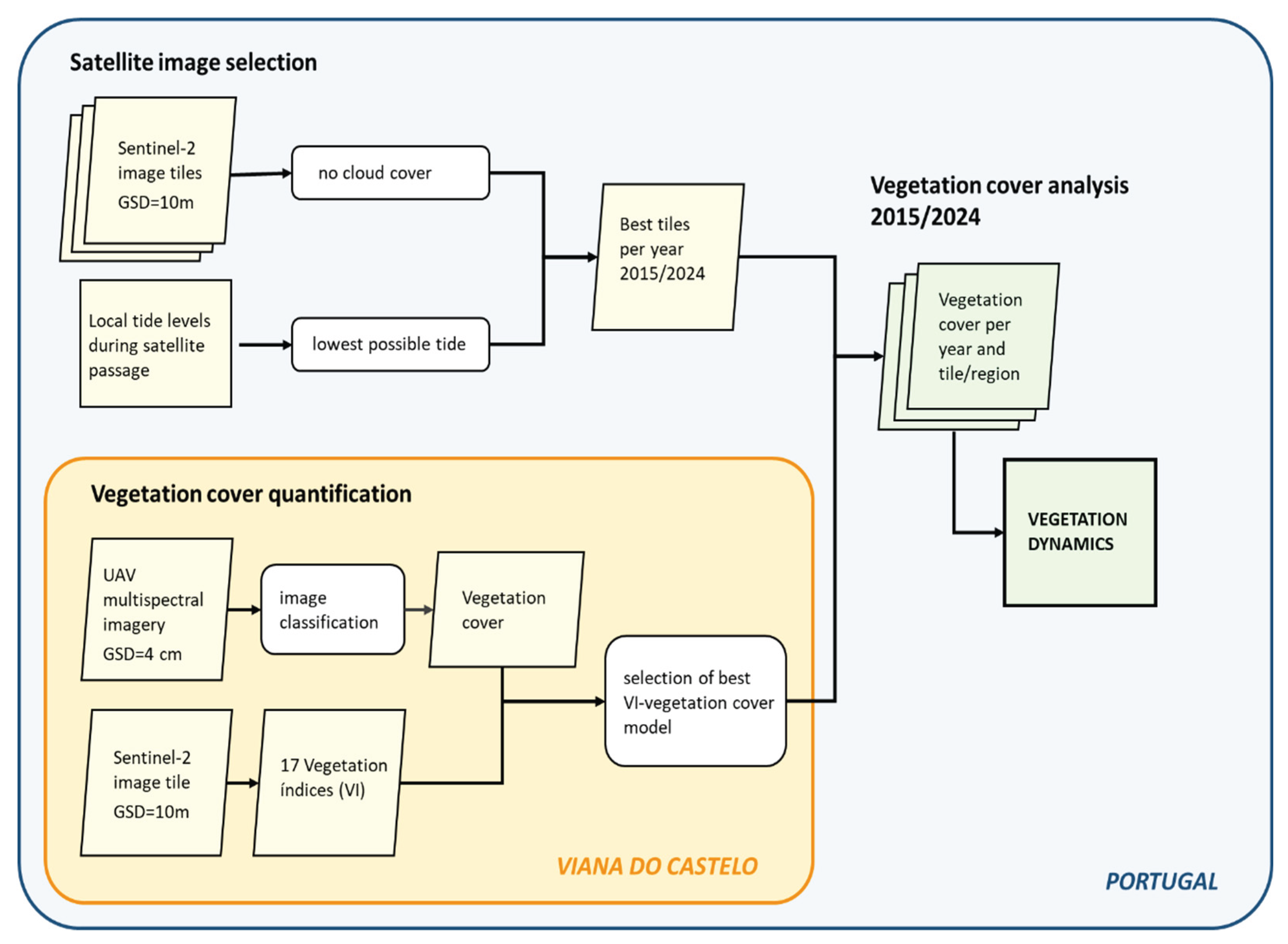
Figure 2.
Location of the study area, the coast of continental Portugal, with the respective Sentinel-2 image tiles, and the validation area near Viana do Castelo (red dot); the intertidal areas are marked in green, showing the three bigger intertidal areas studied: the Minho estuary in the north, the Ria de Aveiro lagoon, and the Ria Formosa in the South.
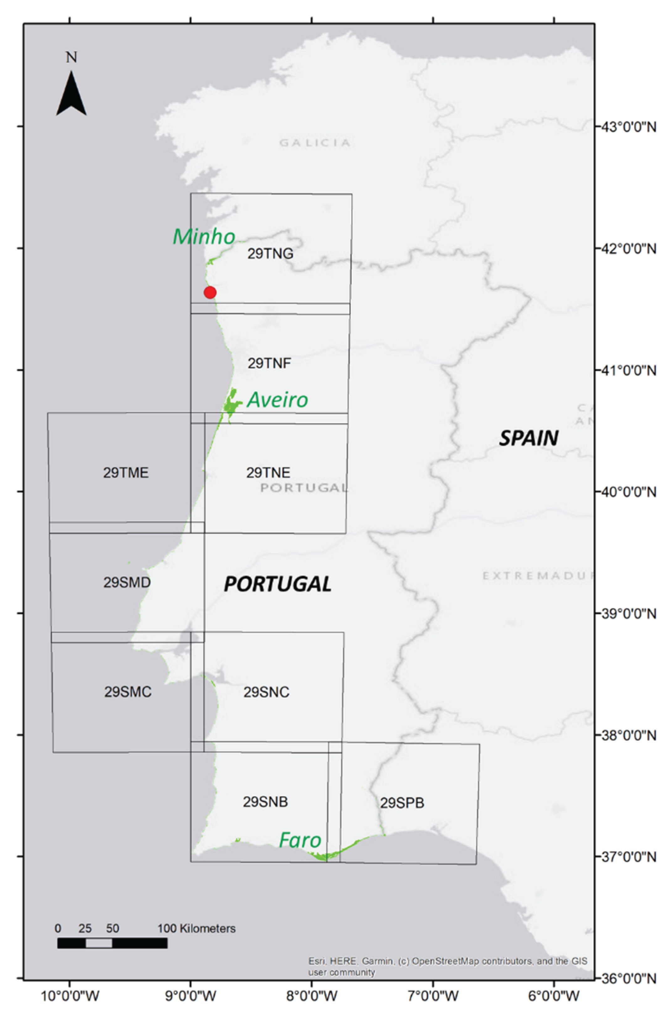
Figure 3.
Orthomosaic of the intertidal area near Viana do Castelo (41° 41′ 45.6” N, 8° 51′ 10.8” W), used for the determination of vegetation cover and the selection of VI (the yellow polygon delimits the area surveyed with a multispectral camera).
Figure 3.
Orthomosaic of the intertidal area near Viana do Castelo (41° 41′ 45.6” N, 8° 51′ 10.8” W), used for the determination of vegetation cover and the selection of VI (the yellow polygon delimits the area surveyed with a multispectral camera).
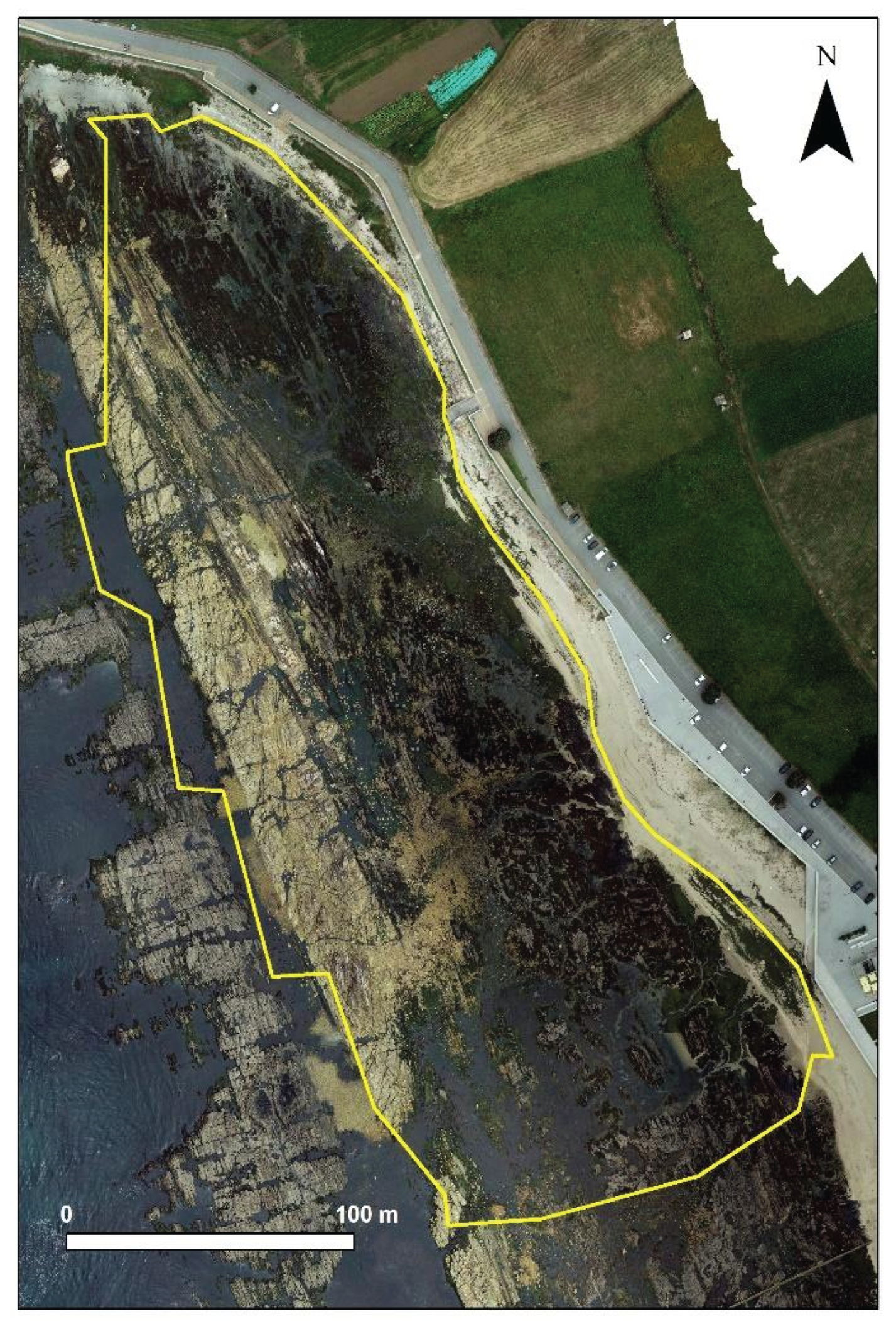
Figure 4.
UAV-image classification results.
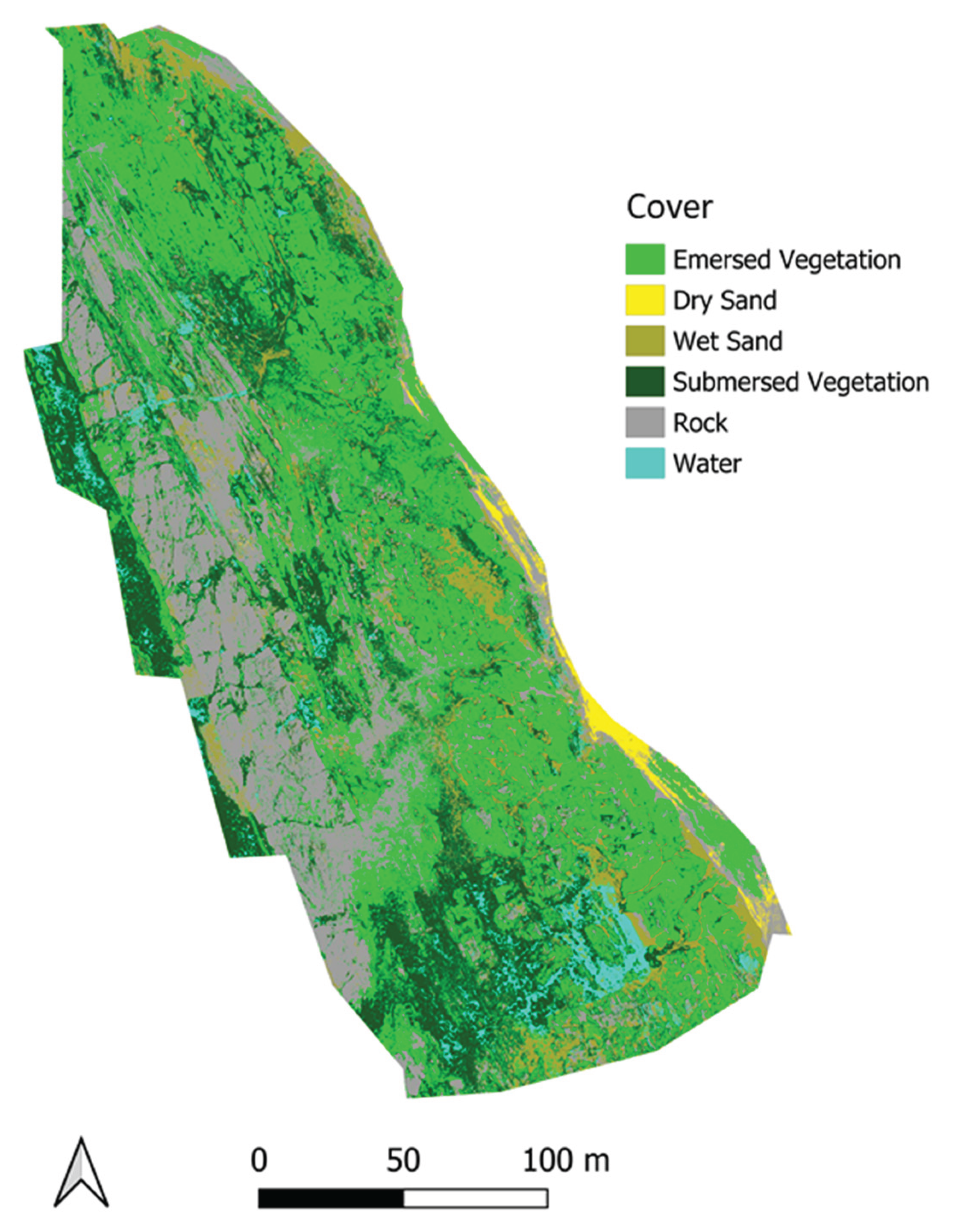
Figure 5.
Best performing model with fitted curve (black line) and 95% confidence intervals (green and red dashed lines).
Figure 5.
Best performing model with fitted curve (black line) and 95% confidence intervals (green and red dashed lines).
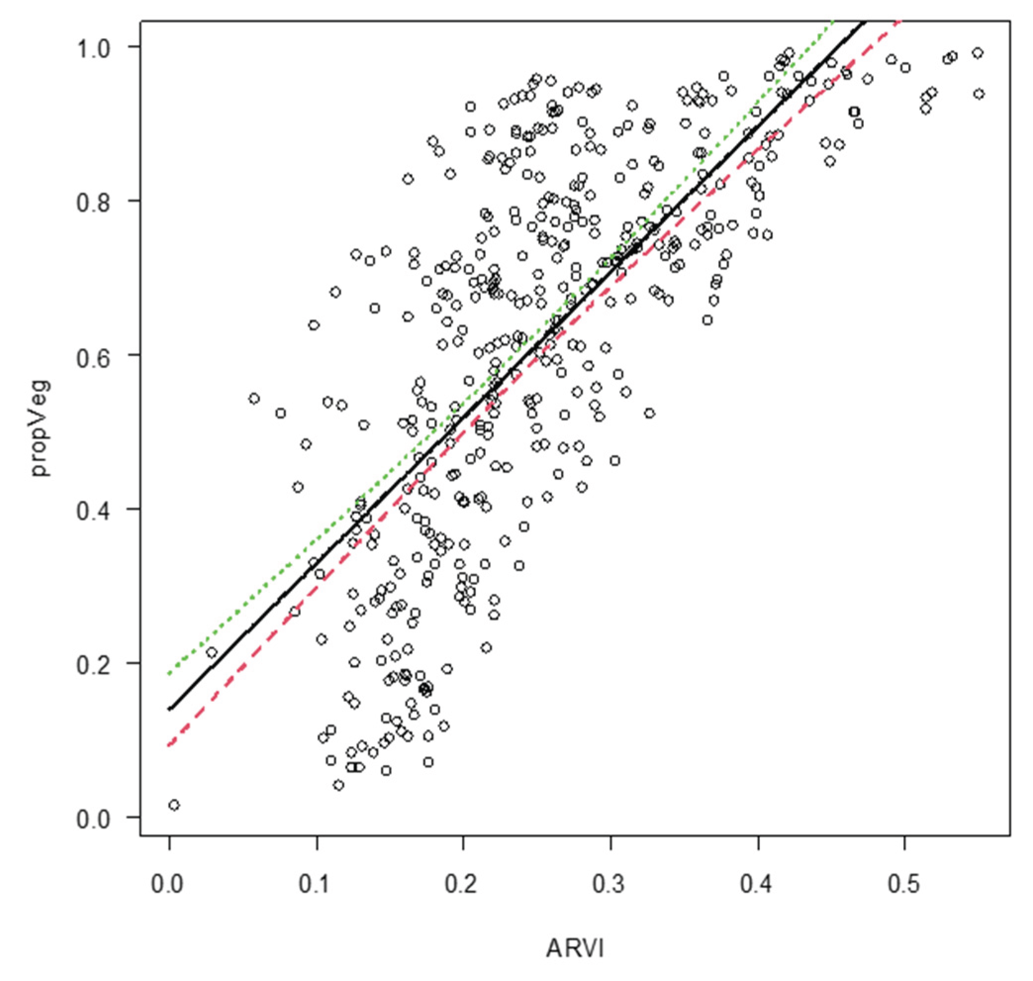
Figure 6.
Estimated vegetation cover over time, in percentage of total intertidal area, per region (a) and estimated vegetation cover area (in ha) for the whole coast, with the blue line representing the tide index, i.e., the weighted average of the water level (astronomical tide) during satellite image capture, weighted by the tiles’ intertidal areas (b).
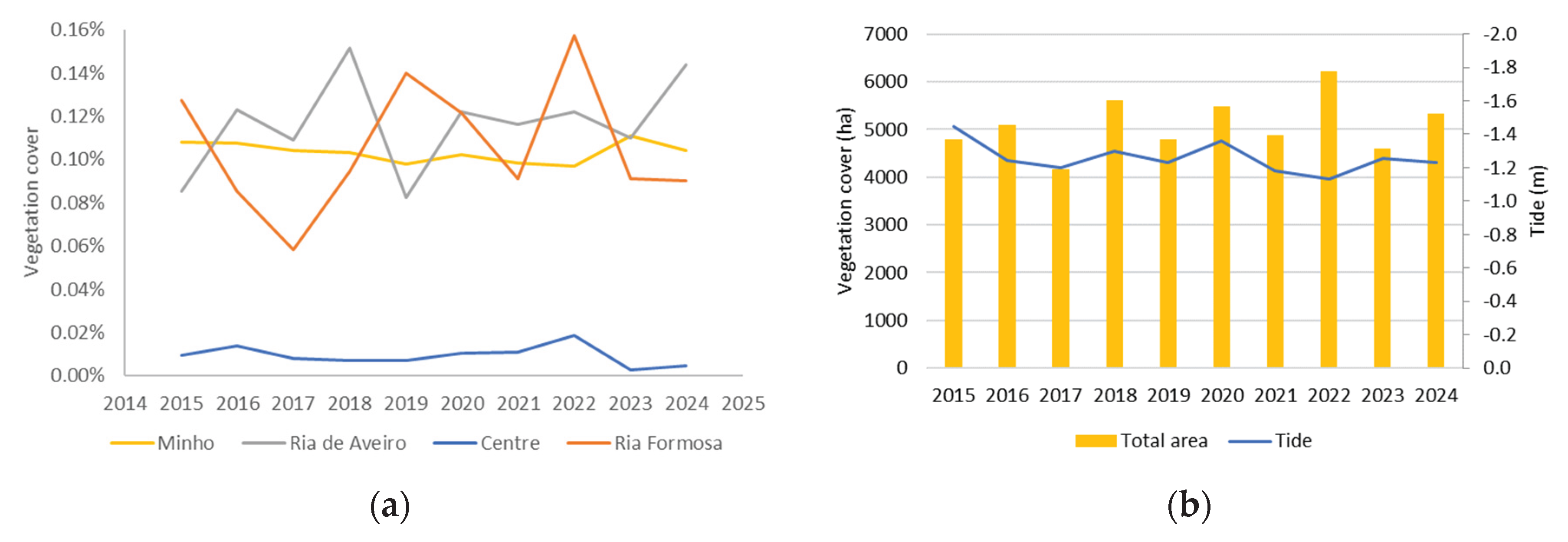
Figure 7.
Intertidal vegetation covers per year for the Minho (a), Ria de Aveiro (b), Centre (c) and Ria Formosa (d) regions; the blue line represents the weighted average of the water level (astronomical tide) during satellite image capture, weighted by tiles’ intertidal areas.
Figure 7.
Intertidal vegetation covers per year for the Minho (a), Ria de Aveiro (b), Centre (c) and Ria Formosa (d) regions; the blue line represents the weighted average of the water level (astronomical tide) during satellite image capture, weighted by tiles’ intertidal areas.
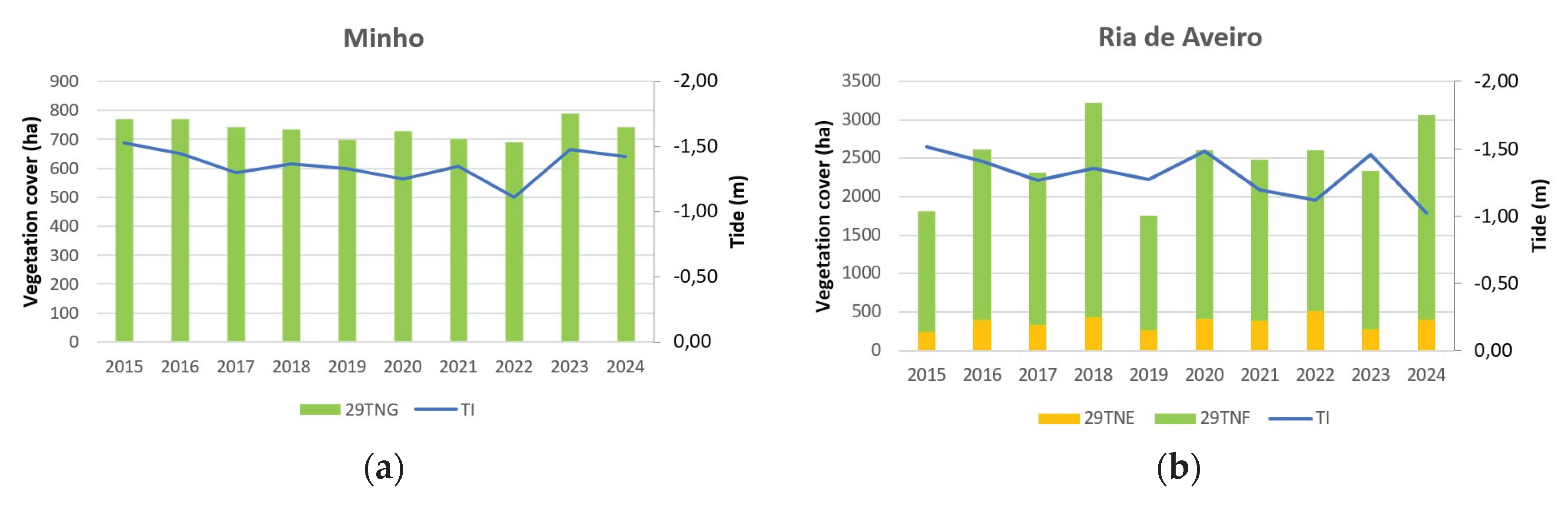
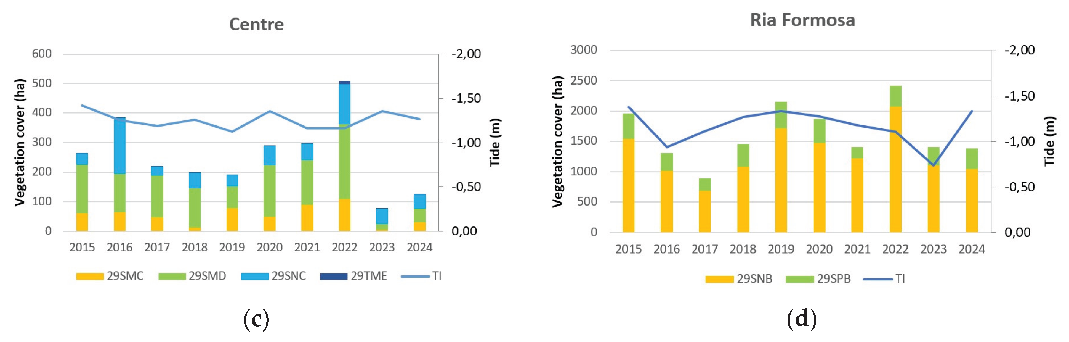
Figure 8.
ARVI values for the Ria de Aveiro lagoon for 2019 (a) and 2020 (b), and the differences between these years (c), with red indicating lower and green higher ARVI.
Figure 8.
ARVI values for the Ria de Aveiro lagoon for 2019 (a) and 2020 (b), and the differences between these years (c), with red indicating lower and green higher ARVI.
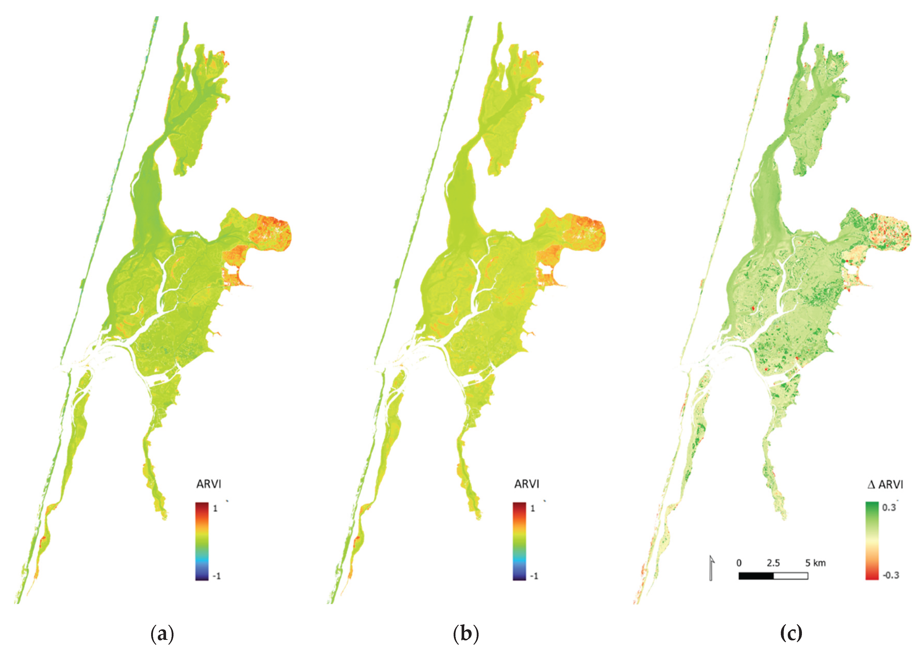
Figure 9.
Intertidal vegetation cover in the Ria de Aveiro Lagoon for 2019 (a) and 2020 (b), and the differences between these years (c), with red indicating lower and green higher ARVI.
Figure 9.
Intertidal vegetation cover in the Ria de Aveiro Lagoon for 2019 (a) and 2020 (b), and the differences between these years (c), with red indicating lower and green higher ARVI.
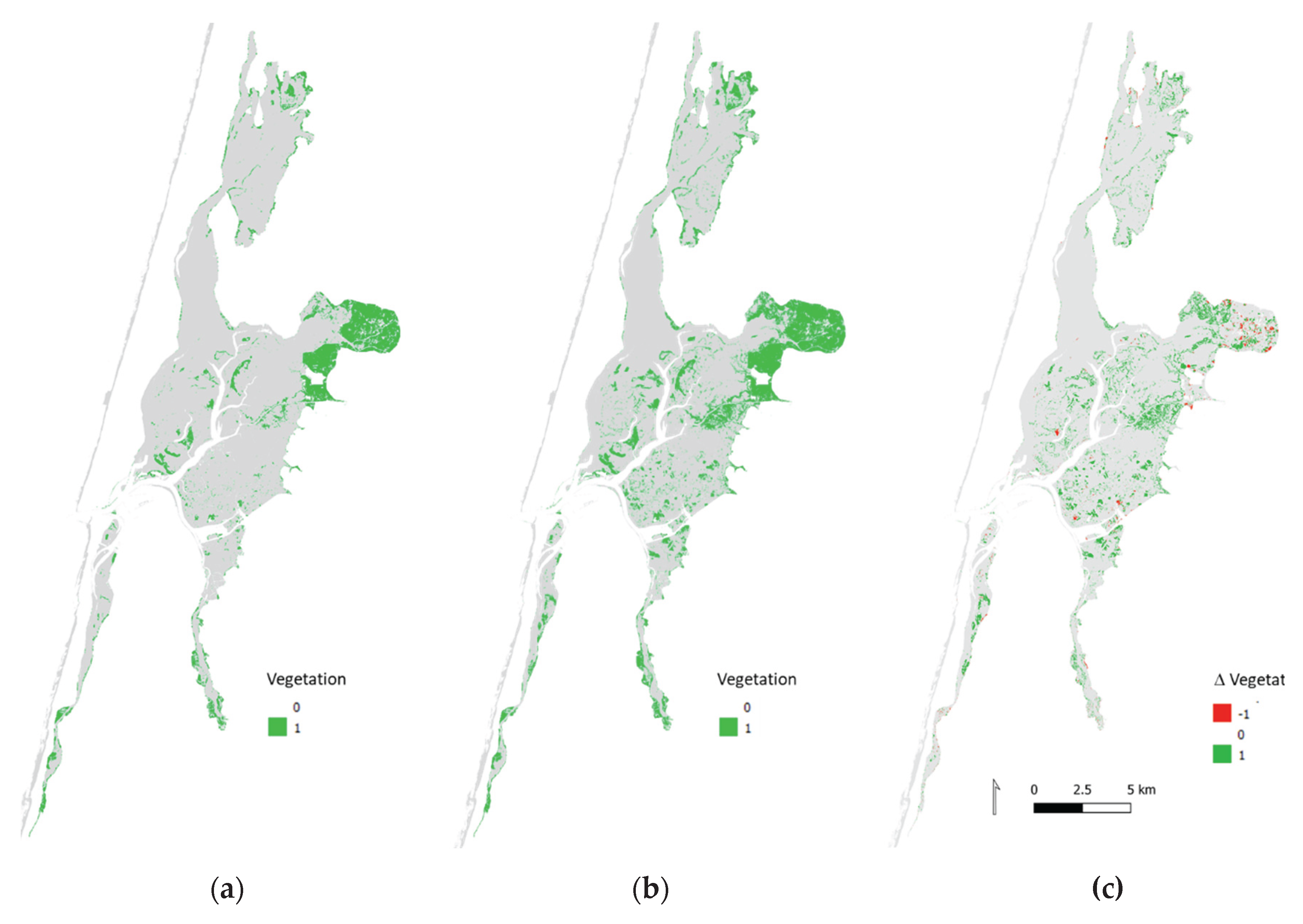
Table 1.
Description of the tested vegetation indices.
| Name | Formula | Reference |
|---|---|---|
| Normalized Difference Vegetation Index | [26] | |
| Renormalized Difference Vegetation Index | [27] | |
| Coastal Redness Vegetation Index | [28] | |
| Difference Vegetation Index | DVI=NIR-Red | [29] |
| Ratio Vegetation Index | [30] | |
| Green Normalized Difference Vegetation Index | [31] | |
| Enhanced Vegetation Index | [32] | |
| Soil Adjusted Vegetation Index | [33] | |
| Normalized Difference Water Index | [34] | |
| Atmospherically Resistant Vegetation Index | [35] 1 | |
| Green Chlorophyll Index | [36] | |
| Red-edge Chlorophyll Index | [36] | |
| Chlorophyll Content Index | [37] | |
| Green Difference Vegetation Index | GDVI=NIR-Green | [7] |
| Enhanced Normalized Difference Vegetation Index | [38] | |
| Modified Green Red Vegetation Index | [39] |
1 Here: using the formula with an atmospheric self-correcting factor y = 1, as Kaufman and Tanre (1992) have shown that when the vegetative cover is sparse and the atmospheric data are unknown (aerosol dimensions), the value of y = 1.0 permits a better adjustment for most remote sensing applications.
Table 2.
Classification results (Veg.: Vegetation).
| Reference Map | ||||||||||
|---|---|---|---|---|---|---|---|---|---|---|
| Emersed Veg. | Dry Sand | Wet Sand | Submersed Veg. | Rock | Water | Total | Area (m²) | Area % | ||
| Classified | Emersed Veg. | 599 | 0 | 0 | 3 | 1 | 0 | 603 | 18003 | 0.377 |
| Dry Sand | 0 | 30 | 0 | 0 | 0 | 0 | 30 | 497 | 0.010 | |
| Wet Sand | 0 | 3 | 122 | 0 | 3 | 3 | 131 | 3902 | 0.082 | |
| Submersed Veg. | 16 | 0 | 3 | 334 | 2 | 12 | 367 | 10995 | 0.230 | |
| Rock | 3 | 19 | 3 | 0 | 383 | 0 | 408 | 12177 | 0.255 | |
| Water | 0 | 0 | 4 | 2 | 0 | 68 | 74 | 2208 | 0.046 | |
| Total | 618 | 52 | 132 | 339 | 389 | 83 | 1613 | |||
| Estimated Area | 18452 | 1154 | 3932 | 10156 | 11610 | 2478 | 47781 | |||
| Area % | 0.386 | 0.024 | 0.082 | 0.213 | 0.243 | 0.052 | ||||
| SE Area | 141 | 137 | 127 | 177 | 162 | 134 | ||||
| 95% CI Area | 554 | 537 | 500 | 695 | 635 | 527 | ||||
| Producer’s Accuracy | 0.969 | 0.431 | 0.924 | 0.985 | 0.985 | 0.819 | ||||
| User’s Accuracy | 0.993 | 1.000 | 0.931 | 0.910 | 0.939 | 0.919 | ||||
| F1 Score | 0.981 | 0.602 | 0.928 | 0.946 | 0.961 | 0.866 | ||||
| Overall Accuracy | 0.952 | |||||||||
Table 3.
Ranking with the best model per VI, showing model formula and adjusted R2.
| VI | Model | Adjusted R2 |
|---|---|---|
| ARVI | lm(propVeg ~ARVI) | 0.517 |
| NDVI | lm(propVeg ~ log(NDVI)) | 0.470 |
| RVI | lm(propVeg ~RVI) | 0.468 |
| GCI | lm(propVeg ~ log(GCI)) | 0.466 |
| GNDVI | lm(propVeg ~ log(GNDVI)) | 0.441 |
| RCI | lm(propVeg ~ log(RCI)) | 0.436 |
| NDWI | lm(propVeg ~NDWI) | 0.424 |
| CVI | lm(propVeg ~ log(CVI)) | 0.364 |
| RDVI | lm(propVeg ~RDVI) | 0.316 |
| SAVI | lm(propVeg ~SAVI) | 0.307 |
| EVI | lm(propVeg ~EVI) | 0.289 |
| ENDVI | lm(propVeg ~ENDVI) | 0.216 |
| DVI | lm(propVeg ~DVI) | 0.207 |
| GDVI | lm(propVeg ~GDVI) | 0.181 |
| MGRVI | lm(propVeg ~MGRVI) | 0.145 |
| CRVI | lm(propVeg ~CRVI) | 0.101 |
Table 4.
Area covered by intertidal vegetation (in ha) from 2015 to 2024, for the Portuguese coast (All) and per region, with respective satellite tile code (see Figure 2).
Table 4.
Area covered by intertidal vegetation (in ha) from 2015 to 2024, for the Portuguese coast (All) and per region, with respective satellite tile code (see Figure 2).
| Year | All | Minho | Aveiro | Centre | Ria Formosa | |||||
|---|---|---|---|---|---|---|---|---|---|---|
| 29TNG | 29TNE | 29TNF | 29TME | 29SMD | 29SMC | 29SNC | 29SNB | 29SBP | ||
| 2015 | 4802.0 | 769.8 | 249.6 | 1561.4 | 61.4 | 164.1 | 37.4 | 0.9 | 1546.2 | 411.2 |
| 2016 | 5083.8 | 769.2 | 405.3 | 2213.0 | 65.4 | 129.1 | 189.7 | 0.3 | 1019.7 | 292.3 |
| 2017 | 4174.9 | 743.5 | 331.3 | 1984.2 | 46.6 | 141.4 | 30.7 | 0.2 | 689.8 | 207.3 |
| 2018 | 5611.2 | 734.9 | 438.1 | 2783.4 | 11.8 | 134.6 | 52.2 | 0.8 | 1088.2 | 367.3 |
| 2019 | 4795.0 | 699.4 | 264.6 | 1488.5 | 78.8 | 72.2 | 39.0 | 0.1 | 1713.3 | 439.2 |
| 2020 | 5492.0 | 729.0 | 416.6 | 2183.4 | 49.6 | 172.8 | 67.3 | 0.1 | 1472.0 | 401.4 |
| 2021 | 4880.7 | 701.5 | 387.6 | 2089.0 | 90.9 | 149.0 | 56.8 | 1.3 | 1226.4 | 178.3 |
| 2022 | 6220.7 | 690.7 | 517.0 | 2083.7 | 109.2 | 253.2 | 135.1 | 11.5 | 2076.5 | 343.7 |
| 2023 | 4606.1 | 790.3 | 281.2 | 2054.9 | 4.4 | 19.9 | 51.5 | 0.4 | 1106.5 | 296.9 |
| 2024 | 5321.0 | 742.1 | 401.3 | 2663.2 | 30.0 | 46.7 | 47.8 | 0.0 | 1044.2 | 345.6 |
Disclaimer/Publisher’s Note: The statements, opinions and data contained in all publications are solely those of the individual author(s) and contributor(s) and not of MDPI and/or the editor(s). MDPI and/or the editor(s) disclaim responsibility for any injury to people or property resulting from any ideas, methods, instructions or products referred to in the content. |
© 2025 by the authors. Licensee MDPI, Basel, Switzerland. This article is an open access article distributed under the terms and conditions of the Creative Commons Attribution (CC BY) license (http://creativecommons.org/licenses/by/4.0/).
Copyright: This open access article is published under a Creative Commons CC BY 4.0 license, which permit the free download, distribution, and reuse, provided that the author and preprint are cited in any reuse.


