Submitted:
28 July 2025
Posted:
20 August 2025
You are already at the latest version
Abstract
This paper introduces a novel framework for designing fair and sustainable unemployment 2
benefits, grounded in cooperative game theory and real-time fiscal policy. We conceptualize 3
the labor market as a coalitional game, where a random subset of individuals is employed, 4
generating stochastic economic output. To ensure fairness, we adopt equal employment 5
opportunity as a normative benchmark and introduce a dichotomous valuation rule that 6
assigns value to both employed and unemployed individuals. Within a continuous-time, 7
balanced budget framework, we derive a closed-form payroll tax rate that is fair, debt- 8
free, and asymptotically risk-free. This tax rule is robust across alternative objectives and 9
promotes employment, productivity, and equality of outcome. The framework naturally 10
extends to other domains involving random bipartitions and shared payoffs, such as voting 11
rights, health insurance, road tolling, and feature selection in machine learning. Our 12
approach offers a transparent, theoretically grounded policy tool for reducing poverty and 13
economic inequality while maintaining fiscal discipline.
Keywords:
payroll tax
; unemployment benefits
; fair division
; continuous-time balanced budget
; dichotomous valuation
; equal employment opportunity
; sustainability
; equality of outcome
; feature selection
; shapley value
1. Introduction
This paper addresses a fundamental issue in economics: not everyone in the labor force can be employed simultaneously. Consequently, while some individuals are employed and receive wages along with employment-related benefits—such as pensions, health and life insurance, social security, and paid leave—others remain unemployed. This reality raises two key questions: 1. Should unemployed individuals receive financial support? 2. If so, what constitutes a fair amount?
In most advanced economies, the answer to the first question is generally “yes.” This paper supports that view, advocating for unemployment benefits for all individuals in the labor market, including recent graduates. In both legal and economic contexts, such financial support may be referred to as unemployment benefits, unemployment insurance, unemployment payments, or unemployment compensation.
To address the second question, this paper proposes a method for fairly distributing unemployment benefits and determining a just payroll tax rate for the employed. The proposed framework ensures a reasonable allocation of a randomly generated economic output between two randomly formed groups within the labor market. A broader objective is to reduce economic inequality and alleviate poverty.
The problem of fair division arises in many real-world contexts. For example, consider a k---n redundant system with n identical components, where the system remains functional as long as any k components are operational. Intuitively, each component—whether active or idle—should be valued equally. A similar principle applies in majority voting systems: even if only some voters support a measure, all voters are assumed to have equal voting power. In the health insurance industry, not all policyholders fall ill or use their coverage, yet the total cost must be fairly shared among both healthy and sick policyholders.
The labor market presents a more complex version of this familiar problem: while not everyone can be employed at the same time, everyone desires employment. Moreover, individuals contribute differently to overall production. Across these varied scenarios, four common features emerge: 1. A cooperative group of participants; 2. A random division of these participants into two subgroups; 3. A payoff resulting from this division; 4. A goal of distributing the payoff fairly among all participants.
This paper develops a framework to address such situations. In systems like the k---n model or majority voting, the desired outcome is equality. The same principle underpins our approach to fair distribution in the labor market.
Determining a fair tax rate and a just distribution of welfare and benefits—both implemented by the employed—presents several challenges. First, while fairness is a central concept, it remains inherently abstract and subject to multiple interpretations. This paper argues that the prevailing social norm should prioritize equal employment opportunity over equal outcomes or productivity.
Second, even when job availability is limited, every individual in the labor market can contribute in some capacity. Unemployment, therefore, should not be viewed as a personal failure or a systemic flaw. Rather, it should be understood as a self-regulating mechanism that enhances labor market efficiency, consistent with search and matching models (e.g., Mortensen and Pissarides, 1994).
Third, applying tax policy to the labor market is complicated by the economy’s dynamic nature and fluctuating productivity levels. For taxation and benefit distribution to be effective, they must be adaptable to uncertainty and sustainable over time. Ideally, these policies should maintain a balance between the value created and the value distributed, even as employment conditions evolve.
In an objective, data-driven framework, a fair tax rate should be determined solely based on observable data. This approach reduces the influence of political negotiations and minimizes the risk of costly strategic voting. However, a major challenge lies in the fact that the heterogeneous-agent production function—which maps all possible combinations of labor participants to economic output—is not directly observable. In practice, we only observe the outcomes of specific labor groupings at discrete points in time. This function is essential for evaluating individual contributions and plays a critical role in assessing benefits and welfare.
Another complication arises from the mismatch in timing between how frequently unemployment data are updated and how often tax rates are adjusted. Unemployment rates are typically reported frequently (e.g., monthly), whereas tax rates are revised less often (e.g., annually). As a result, policymakers often base tax decisions on outdated unemployment data. To address this issue, we propose a fair tax rate model designed for a continuous-time production and employment environment. This model aims to maintain stability in a lower-frequency policy setting by minimizing variability in tax rates.
A substantial body of literature has explored fairness in taxation and unemployment benefits from various perspectives (e.g., Kornhauser, 1995; Fleurbaey and Maniquet, 2006). A foundational contribution is Shapley’s (1953) fairness axiom, which led to the development of the Shapley value—a widely used method for allocating employment compensation and welfare (see Moulin, 2004; Devicienti, 2010; Giorgi and Guandalini, 2018; Krawczyk and Platkowski, 2018). However, the Shapley value relies on two key assumptions: (1) all participants contribute to value creation without division, and (2) the distributor has complete knowledge of the production function.
Recent work by Hu (2006, 2020) relaxes the first assumption and generalizes the Shapley value by introducing non-informative probability distributions to model the division of participants. In this framework, a participant is valued either by their marginal contribution—if directly involved in production—or by their opportunity cost to production otherwise. This dichotomous valuation approach is further developed in Hu (2020), which employs a beta-binomial distribution to represent equal opportunities for participation. While this paper adopts that distribution, many of its results hold independently of it. Crucially, this framework does not require full knowledge of the production function and relies only on a single observed outcome. As a result, both marginal contributions and opportunity costs remain unobservable.
Beyond its extensions to the Shapley value, this work offers three additional contributions. First, while much of the literature on unemployment insurance is empirical or structural, this paper introduces a normative framework grounded in fairness and sustainability. It provides a game-theoretic microfoundation for financing unemployment insurance, complementing or extending standard macroeconomic models. Second, it develops a fair-division solution for a random payoff within a coalitional game framework. This solution is broadly applicable to similar settings with minimal modification and can be adapted using alternative identification schemes beyond those discussed in Section 4. For instance, when applied to feature selection in machine learning, the fair-division approach achieves significantly higher accuracy than many widely used methods. Third, the derived tax rule is simple, interpretable, and robust—qualities essential for real-world policy design. It depends solely on the unemployment rate and a reserved spending rate for common goods and services. Total unemployment compensation is determined entirely by the tax rate and realized production. Under an additional assumption about production, the model also implies equality of outcome, helping to mitigate income inequality. This equality may still hold despite disparities in employment opportunities and productivity among labor force participants.
In addition to methodological innovations such as dichotomous valuation, mixed-frequency analysis, and data-driven approach, this paper embeds policy instruments within a Bayesian framework by linking objectives and constraints to hyperparameters. Moreover, the balanced budget rule is formulated as a functional equation that holds across all labor market contingencies, while the tax solution—expressed as a function of the unemployment rate—is uniquely determined from the equation. In deriving this unique solution, the paper deliberately avoids unnecessary complexity—such as randomness, hypotheticals, ambiguity, and latency. This includes, but is not limited to, competitive and cooperative labor market dynamics, endogenous job search behavior, non-linear tax schedules, precise labor market size, and fluctuations in the unemployed population. While this simplicity entails a degree of abstraction, any real-world application of the fair-division solution should be carefully tailored to its specific context.
The rest of the paper is organized as follows. Section 2 applies the dichotomous valuation (“D-value”) framework from Hu (2006, 2020) to assess the value of each individual in the labor market, assuming equal employment opportunity. The two components of the D-value are aggregated separately for the unemployed and the employed. Section 3 formulates a set of fair allocations of net production using these aggregated D-value components and derives a set of fair tax rates based on two accounting identities that ensure a balanced budget. Section 4 identifies a specific tax rate by either maximizing the stability of the posterior unemployment rate or minimizing its expected value. This solution is shown to be robust under several alternative criteria. Under a productivity assumption, the identified tax rate leads to equality of outcome, as demonstrated in Section 5. Section 6 explores four additional applications of the division rule: voting power, health insurance, highway tolls, and feature selection. Finally, Section 7 concludes with suggestions for extending this framework. The paper is self-contained, and all mathematical proofs are provided in the appendices.
2. Dichotomous Valuation
Before delving into the formal analysis, we introduce some notations. In a general economy, the labor force consists of both employed and unemployed individuals, excluding part-time workers for simplicity. Let represent the set of individuals in the labor force, indexed accordingly.
Let denote the random subset of employed individuals, which varies daily. A specific realization of this random subset is denoted by S. For any subset , let denote its cardinality. For simplicity, we often use lowercase letters to represent cardinalities: n for , t for , z for , and s for both and its realization .
The employment rate is denoted by (unemployment rate). We also use a vinculum (overbar) to denote singleton sets; for example, “” represents the singleton set . Additionally, we use “∖” for set subtraction, “∪” for set union, and for the beta function with parameters and .
2.1. Equality of Employment Opportunity
Equal employment opportunity (EEO) is a widely recognized principle and serves as the foundational axiom for our study of fairness. In the United States, EEO was institutionalized through Executive Order 11246, signed by President Lyndon Johnson in 1965. This order prohibits federal contractors from discriminating on the basis of race, sex, creed, religion, color, or national origin. Similarly, the Equality Act 2010 in the United Kingdom imposes comparable obligations on employers, service providers, and educational institutions.
The literature offers a rich array of both qualitative and formal discussions on the concept of equal opportunity (e.g., Friedman and Friedman, 1990; Roemer, 1998; Rawls, 1999). Given the multiple interpretations of equality, it follows that there are many definitions of fairness—and consequently, numerous possible fair tax rates.
Many scholars interpret fairness or justice as equality of opportunity, particularly in the context of distributive justice and economic outcomes. A comprehensive review by Alms (2023) explores fairness preferences and beliefs about inequality, emphasizing that equality of opportunity is a core principle of justice. According to this view, differences in outcome are unfair if they arise from factors beyond personal responsibility, but fair if they result from individual’s choices and efforts. Joseph (1980) examines various conceptions of equality of opportunity, distinguishing it from equality of outcomes. He frames equality of opportunity as a form of procedural fairness, where access to positions is based on merit and free from discrimination. In Rawlsian theory (e.g., Segall, 2014), fair equality of opportunity is a foundational element of justice. It asserts that individuals with similar talents and willingness to apply them should have equal chances to attain desirable positions, regardless of their social background.
Beyond the justification rooted in EEO, unemployment compensations can also be supported by other rationales, including social protection, income flow insurance, poverty prevention, and political considerations (e.g., Sandmo, 1998; Tzannatos and Roddis, 1998; Vodopivec, 2004).
In this study, we introduce a probabilistic version of EEO, where employment opportunities are assumed to be equitably distributed among all individuals in the labor force. Under a distribution-free EEO framework, the probability that any individual is employed (i.e., ) is given by for all . However, the proportion itself varies over time. Beta distributions are commonly used to model proportion data (e.g., Ferrari and Cribari-Neto, 2004) due to their continuous range over the interval , flexible shape, role as conjugate priors in Bayesian analysis, and applicability in regression models with unknown parameters.
Given that both n (the total labor force) and s (the number of employed individuals) are nonnegative integers, we model the randomness of the employed subset using a three-layered uncertainty framework:
- First Layer: The size of the employed subset follows a binomial distribution with parameters , where p is the probability that any given individual is employed.
-
Second Layer: The employment probability p is treated as a random variable with a beta prior distribution characterized by hyperparameters . The joint probability density of p and is given by:This implies that the marginal probability of observing t employed individuals is:for any
- Third Layer: Given an employment size t, all subsets of size t are equally likely to be the employed group . Since there are such subsets, the probability of a specific employment scenario is:
This three-layered uncertainty model ensures that every individual in the labor market has an equal probability of being employed. While this assumption may seem somehow unrealistic—given the realities of structural unemployment and skill mismatches—it is important to clarify that this interpretation of EEO does not imply perfect labor mobility. That is, it does not assume that workers can move freely between jobs, industries, or locations without barriers or costs.
Moreover, EEO does not suggest that all workers are identical; production still requires a heterogeneous workforce. Nor does it imply that all applicants have an equal chance at any specific job. Hiring decisions remain at the discretion of employers, who select candidates based on their suitability for specific roles.
EEO is more likely to be realized in labor markets characterized by high market depth, strong labor mobility, low structural unemployment, and minimal skills mismatch. Diversity and inclusiveness also play a crucial role in enhancing EEO by bridging gaps across different types of positions. In such inclusive markets, opportunities are accessible to all—including recent graduates who begin in entry-level roles and build experience toward their ideal careers.
To uphold EEO, governments can take several proactive measures. These include stimulating job creation across diverse industries to balance labor supply and demand, offering free training programs for unemployed individuals in high-demand fields, and developing efficient job-matching platforms to connect job seekers with emerging opportunities, particularly as these opportunities shift across sectors. Female labor participation often lags behind that of males. In response, numerous fiscal policies have been implemented in recent decades to promote greater inclusion. Professionals can leverage these evolving dynamics to advance their careers or transition into roles that better align with their skills and aspirations.
Since the employment rate results from the interaction of labor demand and supply, the hyperparameters of the beta distribution can be interpreted as representing the intensity of demand and supply, respectively. Consequently, represents the overall intensity of the labor force—that is, labor force participation. Explanatory variables may be linked to these intensities. In particular, and can serve as as policy instruments through which constraints are imposed and objectives are defined. Their influence is reflected in the posterior employment rate, which emerges from both policy intervention and observed outcomes. Based on the profile of this posterior rate, we solve the problem in reverse to determine an optimal policy rule.
According to Eqs. (1) and (2), the posterior density function of p, given , is:
Thus, the posterior employment rate follows a Beta distribution with parameters . We denote this posterior employment rate as , given the observation of n and . In contrast, p remains an unobservable parameter for the binomial random variable .
2.2. Aggregate Values of the Employed and the Unemployed
For any subset , we define a heterogeneous-agent production function to measure the net aggregate production generated by the employed group S. The function represents net profit, excluding labor costs—these costs compensate individuals for their time and efforts. To isolate the value added by labor, also excludes the cost of consumed physical and financial resources. Both labor and resource costs are exempt from taxation. Without loss of generality, we assume for the empty set ∅. Importantly, does not necessarily increase with the size of S; in fact, a certain level of unemployment may enhance productivity.
To retain labor and minimize turnover, firm often share a portion of their net profit with employees. For simplicity, we refer to this shared portion of as employment welfare, distinguishing it from unemployment benefits, which are provided to those not currently unemployed. Employment welfare plays a critical role in employee retention and business continuation—both of which significantly influence productivity. The longer employees remain in their roles, the more skilled and efficient they become, and the fewer costly mistakes they make. In contrast, new hires typically require months to acclimate and years to reach full proficiency. As key contributors, firm owners also claim a share of to compensate for their risk-bearing investments, entrepreneurial efforts, and financing costs.
We now formally introduce the components of the D-value. For any individual , we analyze their marginal effect on the value-generation process by considering two mutually exclusive and jointly exhaustive events:
- Event 1: (i.e., the individual is currently employed). In this case, the marginal contribution of i is given by the difference , referred to as the marginal gain. This represents the value added by individual i due to their presence in the employed group . The expected marginal gain is defined as:where “” denotes definition and “” represents the expectation with respect to the probability distribution of .
- Event 2: (i.e., the individual is currently unemployed). This may occur if the individual has just entered the labor market (e.g., after completing school) or is experiencing cyclical, structural, or frictional unemployment. In this case, the marginal contribution is , representing the marginal loss due to the absence of i from the workforce. If i were included in , production would increase by this amount. The expected marginal loss is defined as:
Let denote the employment welfare received by individual i when employed, and the unemployment benefits received when unemployed. Note that even if i remains continuously employed, the sets and evolve over time, so the marginal gain is not constant. Similarly, if i remains unemployed, the sets and , and thus the marginal loss, also vary. To account for this uncertainty, we define and as expectations, as shown in Eqs. (4) and (5).
The valuation framework primarily emphasizes the labor force, often overlooking the contributions of other stakeholders. Several implicit considerations underlie this approach:
- Compensation for Human Capital: In addition to receiving employment welfare, employed individuals are compensated for their labor. This compensation reflects the value of human capital used in generating . Human capital is developed not only through current employment but also through prior work experience and pre-employment education. In contract, unemployed individuals receive only unemployment benefits.
- Observability of Marginal Contributions: When , the value is unobservable; we can only observe . Similarly, when , we cannot simultaneously observe both and . Therefore, it is necessary to transform aggregate marginal values into observable forms, as outlined in Theorem 1.
- Redistribution of Surplus: The total employment welfare, , does not equal the total value . As a result, some of the surplus is redistributed to the unemployed individuals in . This redistribution occurs not through direct transfers, but via government taxation and unemployment benefit systems. This mechanism also supports national-level welfare and benefits, as formalized in Theorem 1.
Theorem 1.
The aggregate components of the D-value are given by:
and
The coalition realizes the value , but it could not have achieved this value independently—support from the broader society and the entire labor market is essential. Accordingly, the government holds the authority to influence aggregate outcomes, as outlined in Theorem 1, by adjusting the hyperparameters and . This control enables the specification of budgetary constraints and the formulation of optimal fiscal policies. Moreover, substituting certain individuals in with those from may yield the same or even greater value. Although most jobs are functionally replaceable, neither Eq. (4) nor Eq. (5) captures the value added when replacing individual i with another individual j from either or , respectively.
As demonstrated in Theorem 11 of Hu (2020), when (i.e., when p follows a uniform distribution on ), the Shapley value of player i in the coalitional game equals the sum . Furthermore, if we impose the functional equation (or ), then (or , respectively) corresponds to player i’s Shapley value (cf. Hu, 2020). However, these conditions are generally unrealistic in actual labor markets.
3. Accounting Identities for a Balanced Budget
According to Eq. (3), the expected production is given by:
where the probability of each employment scenario is determined by the hyperparameters and . At any given time, only one of the possible employment scenarios is realized. The specific scenario occurs with probability and yields a value . This is the value available for allocation when scenario occurs. In contrast, the Shapley value distributes the total value among all players in . Hu (2020) proposes solutions for distributing the expected value among all participants. Additionally, the literature on unemployment insurance financing (e.g., Hopenhayn and Nicolini, 1997) frequently addresses how to fund such insurance in a sustainable manner.
3.1. A Real-Time Balanced Budget Rule
Our division rule must fully respect all entitlements to . Each employed individual receives their expected marginal gain, , and each unemployed individual receives their expected marginal loss, . Additionally, a portion is reserved for common goods and services—supporting the broader economy and society, which in turn sustain the value-generating process. Thus, the profit-sharing strategy divides the realized net production into three components:
- Public Reserve: A reserved proportion is set aside for collective societal and economic purposes. This portion is not distributed directly to individuals.
In summary, the allocation rule sets up a functional equation:
for the random variable , a measurable function from to real numbers. That is, the equation holds for any of the realized values of . Also, by Eqs. (6) and (7), allocations to and are determined through the formula:
This differs from . Since only one is revealed or realized, it is impossible to determine the exact value of . However, the revealed serves as both the maximum likelihood and the least squared estimate of .
We define the tax rate as:
This rate does not directly depend on the production function . The tax revenue is used to fund both unemployment benefits and a reserve fund. Therefore,
Unemployment benefits can be managed either independently or in conjunction with taxation, depending on the country. For example, in Australia, unemployment benefits are part of the broader social security system and are funded through general taxation. In the United States, a compulsory government insurance system manages unemployment benefits, including both the collection and disbursement of funds. In addition to the Federal Unemployment Tax Act, individual states administer their own unemployment insurance programs, resulting in variation in tax rates across different years and states.
The reserve portion serves the broader public interest rather than individual needs. Specifically, it may fund—but is not limited to—programs and services such as support for individuals outside the labor force, Social Security and Medicare, public administration and national defense, public services, and servicing of past tax deficits, including interest payments. In the United States, Social Security and Medicare are managed separately and funded through flat tax rates, which are not adjusted based on gross household income—unlike progressive income tax systems.
The continuous-time balanced-budget rule prohibits borrowing or lending across different labor market scenarios and over time. This sustainable taxation policy is designed to meet the needs of the current market scenario while preserving the capacity of future scenarios to meet their own needs. Importantly, excessive taxation that results in budget surpluses can also have adverse effects: it may raise consumer prices, reduce output, and stifle competition. These outcomes can lead to a suboptimal allocation of resources, creating deadweight loss and diminishing overall economic efficiency.
Democratic governments often face challenges in maintaining long-term budget balance. Successive administrations may lack the incentive to address debt inherited from their predecessors. When GDP is measured using the expenditure approach, governments may choose to finance crises and wars through debt and increased spending in an effort to sustain GDP growth. Political competition can also lead to unsustainable tax cut aimed at appealing to specific voter groups. Over time, such practices contribute to rising debt levels and tax policies that imposes burdens on future generations. In contrast, our real-time budget balance framework holds the current administration accountable for the debt it incurs. Unlike the government’s one-time distribution of net production, households can optimize their utility through intertemporal strategies such as borrowing, saving, lending, and consumption.
In practice, implementing a balanced-budget rule at the level of labor market scenarios—or in real time—is challenging. This difficulty arises from the mismatch in frequency between labor market fluctuations and tax rate adjustments. For example, in the United States, the employment rate fluctuates daily and is reported monthly by the Bureau of Labor Statistics, whereas the tax rate is typically adjusted only once per year. To maintain budget balance as effectively as possible, one strategy is to minimize the variance of the employment rate within a given year. Ideally, this rate would follow a degenerate probability distribution—remaining nearly constant throughout the year.
3.2. The Set of Feasible Solutions
For a given triple , there are three unknowns—, and —in a system of two equations, Eqs. (9) and (10). Let denote the set of all feasible combinations that satisfy both budget constraints:
There is inherent uncertainty regarding the size of the labor market n. Although n is not treated as a random variable under the EEO assumption, it is considered a time-varying latent variable. This is due to the lack of a clear boundary between entering and exiting the labor force, and the fact that many unemployed individuals may not be actively seeking employment. Some may also remain unemployed by choice, opting to forgo lower-paid positions.
Despite its variability and latency, the labor force size n is generally large in macroeconomic contexts. Therefore, in addition to solving Eqs. (9) and (10) for specific values of n, we also aim to derive a tax rule that remains valid for all sufficiently large values of n. We define:
if this limits exists for a sequence . For simplicity, we refer to this limiting value as the “-rate,” representing the asymptotic behavior of the tax rate that satisfies the budget constraints.
Eqs. (9) and (10) form a system of linear functions in the variables and , expressed in terms of n, , , and . For notational simplicity, we introduce the following shorthand expressions:
All these expressions are bounded since . Lemma 1 (used in the proofs of subsequent theorems) provides a method for extracting and from Eqs. (9) and (10).
Given that and in Eq. (11), we require to ensure that both and remain positive for large but finite values of n. Consequently, Corollary 1 states that a government should levy at least of the production as payroll tax.
Corollary 1.
The minimal ϕ-rate is .
The posterior employment rate, , reflects a balance between observed data and policy-specified prior expectations. As the volume of data increases, the influence of the prior diminishes significantly. Accordingly, Theorem 2 states that converges to a degenerate distribution as , provided that . This implies that a fixed tax rule does not affect the central tendency of , as long as the tax rate satisfies . This result motivates further exploration of other properties of , such as its variance, rate of convergence, and behavior under varying tax rates—especially given that the labor force size n is finite, regardless of its magnitude.
Theorem 2.
For any ϕ-rate , as , the posterior employment rate converges in distribution to a degenerate probability distribution concentrated at ω.
To derive a unique solution from the set or its limiting boundary, an additional constraint must be imposed, as infinitely many solutions exist for a given triple . One approach is to leverage the statistical relationship between p and the hyperparameters : the mean and mode of p are and , respectively (see Johnson et al., 1995, Chapter 21). For example, one might set either the mean or the mode equal to the average employment rate from the previous year. Alternatively, these expressions could be aligned with a target or natural employment rate. However, this identification strategy requires additional input. Historical averages may not reflect recent trends, natural rates are prone to estimation errors, and target rates may be unattainable.
An alternative approach involves determining a tax rate that maximizes certain properties of , such as its expected value for large but finite values of n. If the -rate depends on the realized value of p, rather than its unobservable uncertainty, a natural way to eliminate this uncertainty is to analyze the posterior rate , treating as fixed while allowing and to remain at the decision-maker’s discretion.
Although provides informative insight into the central tendency of the posterior labor market as , other critical aspects of the full profile of include its asymptotic dispersion and the labor market’s response to the -rate —especially when n is large but finite. Therefore, optimal criteria over the domain can still be established by minimizing dispersion or optimizing the expected market response. For instance, selecting the -rate that minimizes dispersion results in the fastest convergence to the degenerate distribution described in Theorem 2. This approach helps bridge the frequency gap between the daily employment rate and the annually adjusted tax rate .
4. An Optimal Fair Tax Rate
In this section and the next, we derive the minimal -rate from multiple perspectives. A well-designed distribution of benefits should not compromise market efficiency, and an effective tax policy must preserve incentives for employment and productivity, as emphasized in Theorems 5 and 7. At the same time, a robust and optimal tax rule should satisfy several key criteria. Accordingly, we examine five such criteria in Theorems 3, 4, 5, 6, and 8—each of which independently identifies the same solution. Together, these criteria aim to either minimize employment market risk or maximize expected employment, all while respecting the constraints of market capacity and budget balance.
The formulation of this tax rule is grounded in observed market behavior. While an efficient labor market enhances productivity , a higher employment rate does not necessarily imply higher productivity—and vice versa. Acemoglu and Shimer (2000) argue that a moderate level of unemployment can actually improve productivity by enhancing job quality. Unemployment can foster peer pressure to increase output, facilitate the reallocation of labor from declining firms, and enable growing companies—and the broader economy—to respond more effectively to external shocks. Therefore, our proposed tax rule does not aim merely to maximize the employment rate. Instead, it is rooted in empirical market behavior and is designed to enable the market to achieve the highest feasible employment rate within the constraints of budgetary discipline and market capacity.
4.1. Asymptotic Risk-Free Tax Rate
A stable tax rate creates a favorable environment for maintaining a balanced budget, reducing labor market uncertainty, and encouraging investment in both technology and human capital. As a function of the employment rate , the tax rate serves as a mechanism for transmitting risk from fluctuations in unemployment to fiscal policy.
In the absence of external shocks, a stable tax rate effectively corresponds to a stable unemployment rate. However, directly targeting a stable employment rate does not eliminate its variability, as it remains susceptible to numerous shocks. Instead, a well-designed tax policy can mitigate the magnitude of these risks and address the inequities that raise from the mismatch in timing between the frequently changing employment rate and the typically annual adjustment of the tax rate . For instance, if is high in the first half of the year and low in the second, a constant tax rate throughout the year ensures equal payment to unemployed individuals in both periods. However, under a tax rule such as the -rate , the unemployment benefits may still differ between periods.
Theorem 3.
The ϕ-rate minimizes the asymptotic variance of the posterior employment rate , that is:
and the minimum limiting variance is zero.
When the variance of is used as a measure of instability, Theorem 3 demonstrates that the -rate tax rule minimizes this asymptotic variance. However, several clarifications are necessary:
- Limit Behavior: The stability described is achieved only in the limit as , where the variance approaches zero. In practice, remains subject to exogenous shocks, as discussed by Pissarides (1992) and Blanchard (2000). Therefore, the minimum limiting variance is greater than zero.
- Practical Adjustment: While is the limiting tax rule, for large but finite n, a small positive adjustment may be added to ensure the positivity of and . For example,ensures that the denominators in Eq. (11) remain positive, thereby guaranteeing and . This adjustment becomes negligible as n grows large.
- Labor Mobility: With near-zero variance in the unemployment rate, labor mobility implies that layoffs and new hires nearly offset each other, keeping the total employment size s nearly constant. It also means that the number of employed individuals s changes proportionally with the labor market size n. Consequently, the employment rate remains stable.
- Asymmetric Risk Minimization: Although the posterior distribution is skewed, the -rate tax rule minimizes both total and one-sided risks in , as further elaborated in Theorem 4. Policymakers are particularly concerned with downside risk.
Theorem 4.
As , the ϕ-rate minimizes both the lower and upper semivariance of where .
4.2. Consistency and Robustness
The -rate captures several essential features of the labor market. First, it represents the policymaker’s optimal response to stimulate employment while satisfying the constraints of Eqs. (9) and (10). Traditional unemployment insurance literature (e.g., Baily, 1978; Chetty, 2006) emphasizes the trade-off between income smoothing for the unemployed and incentives to search for work. Second, this tax rule can also be derived by minimizing statistical dispersion measures that are more robust than variance or semivariance. Additionally, it contributes to reducing income inequality. Importantly, the tax policy is predetermined before any specific economic scenario unfolds. This transparency reduces both the size and influence of government, which might otherwise spend months deliberating over tax schedules. It also prevents opportunistic behavior, such as favoring certain employment scenarios or manipulating unfavorable ones to justify debt.
The rule represents an effective taxation strategy that maximizes employment without compromising equal opportunity or budget balance. For policymakers, a central concern is the forward-looking employment profile . Unlike Theorem 2, which considers the limit as for a fixed , Theorem 5 holds n fixed and allows to vary. According to Theorem 5, the mean of decreases as increases, for any fixed, large n. Therefore, to maximize the posterior mean, the tax rate should be minimized—while still satisfying the conditions , with , and . Thus, the -rate that maximizes the mean of is The condition in Theorem 5 is typically met in real-world economies.
Theorem 5.
For any and a finitely large n, the mean of decreases as the ϕ-rate increases. Consequently,
Moreover, this tax rule also minimizes the mean absolute deviation (MAD) from the mean as . For Beta distributions—especially with large parameters—MAD is a more robust measure of dispersion than variance or semivariance.
The MAD for the posterior is given by (see Gupta and Nadarajah, 2004, p.37):
Theorem 6.
The ϕ-rate minimizes the asymptotic MAD of , that is:
5. Labor Productivity and Equality of Outcome
An individual’s productivity is shaped by their workplace environment. For any individual , their productivity within reflects how consistently and efficiently they complete tasks and achieve goals. However, actual performance—measured as —depends on the specific composition of the group . When comparing two individuals, one may outperform the other in certain scenarios but not in others. Even with a fixed group size s, the overall production varies with the composition of the group.
At the macroeconomic level, individual productivity does not always align with national productivity, since the marginal contribution does not perfectly correlate with total output . However, under the proposed distribution rule for , aggregate employment welfare aligns exactly with total production for a given tax rate . This alignment incentivizes labor market efficiency. Meanwhile, the imperfect alignment of individual incentives fosters labor mobility, which further enhances overall efficiency.
To connect personal productivity with incentives, we introduce a partial ordering in the labor market. For any two individuals with , we say that individual iuniformly outperforms individual j in productivity v if the following two conditions hold:
4.5in
- for any ; and
- for any with .
These conditions imply that individual i has higher marginal productivity than individual j in all comparable employment scenarios—whether both are employed or both are unemployed.
Since productivity plays a central role in Eqs. (4) and (5), individual j should receive less employment welfare and fewer unemployment benefits than individual i. This principle is formalized in Theorem 7. Importantly, the theorem does not rely on the beta-binomial distribution from Eq. (3), as long as individuals i and j have equal employment opportunity. Other individuals in the labor market may still face unequal opportunities. Moreover, the theorem holds for all tax rates, including the specific -rate: .
Theorem 7.
If individual uniformly outperforms individual in production v, and both have equal employment opportunity, then and .
We say that individuals i and j are symmetric in the production function v if they uniformly outperform each other. According to Theorem 7, if i and j are symmetric and have equal employment opportunity, they should receive the same amount of unemployment benefits when both are unemployed, and the same amount of employment welfare when both are employed.
While the assumption of bilateral symmetry or uniform outperformance is conceptually appealing, it is often overly idealized. In practice, it is not necessary for individual i to uniformly outperform individual j; it is sufficient if the probability that i performs better than j—that is, —is significantly high, or if i is a fast learner, capable of quickly acquiring the necessary skills. Factors such as education, interest, motivation, and experience all influence this probability. Skilled job interviewers can often estimate these probabilities effectively.
In large and medium economies, it is impractical to apply or to allocate individual welfare or benefits. The complexity and scale of economic activities make it difficult to estimate these values accurately. Instead, individual payoffs can be determined by market forces, while ensuring that the overall employment welfare remains within the desired range of and aggregate unemployment benefits are about . By making reasonable assumptions about productivity levels and EEO, a more nuanced approach can be devised. This method overlooks various economic factors and individual contributions but allows for a simpler allocation.
In the absence of detailed analysis or prior knowledge about the production function v, assuming symmetry among the unemployed (or the employed) can serve as a reasonable a priori basis for distributing unemployment benefits (or employment welfare, respectively). For instance, the Cobb-Douglas production function assumes symmetry among all employed individuals. In many real-world systems—such as in the United States—unemployment insurance benefits are not strictly proportional to the amount an individual has contributed. Instead, benefits are typically determined by recent earnings history, state-specific formulas and caps, and eligibility criteria. These systems function more as social insurance mechanisms than private insurance models, prioritizing income smoothing and poverty prevention over strict actuarial fairness.
Both group symmetry and EEO reflect the principle of the veil of ignorance. Under this hypothetical veil, policymakers are unaware of their own social status, wealth, employment condition, productivity, or other personal characteristics. This perspective compels them to design a fair system that applies equally to all individuals, regardless of their future circumstances (cf. Rawls 1999). EEO can also be justified by the principle of insufficient reason (also known as the principle of indifference), which assigns equal probabilities to all competing scenarios of when there is no basis for favoring one over another.
Assuming EEO and symmetry among both employed and unemployed individuals, the -rate tax formula eliminates income inequality when income is defined as the sum of employment welfare and unemployment benefits. Theorem 8 confirms this equality of outcome. Importantly, the theorem imposes no restrictions on the size of the labor force n, nor on the specific probability distribution used to model EEO—though the -rate is derived from the EEO condition defined in Eq. (3).
Theorem 8.
Assume EEO and symmetry among the employed in , and also EEO and symmetry among the unemployed in . Then, if and only if employment welfare equals unemployment benefits.
The theorem remains valid even when employed and unemployed individuals differ in the production function or face unequal employment opportunities. In practice, the employed group tends to have higher average employment probability and productivity than the unemployed group. This disparity is an outcome of market mechanism, not an a priori assumption. These posterior variations in EEO and productivity reflect market efficiency and contribute to overall economic efficiency.
6. Applications and Labor Costs
The preceding analysis has focused on a normative policy framework—one that incorporates value judgments and prescriptive perspectives on how policy should function, rather than emphasizing empirically testable claims. Accordingly, this section does not attempt to validate the division rule using real-world data. Instead, it presents several alternative applications to demonstrate the broader utility of the proposed approach.
In abstract terms, the earlier sections offer a fair-division solution within the following game-theoretic context: players are randomly divided into two groups, each granted equal opportunity, and the random payoff to be allocated originates from one of these groups. This type of model has wide-ranging applications. In this section, we explore four such examples to illustrate the practical relevance of the previously derived formulas. Additionally, we introduce methods for estimating labor costs and the reserve ratio .
6.1. Voting Rights
In a voting game (e.g., Shapley, 1962), the function is a monotonically increasing set function. Let denote the random subset of voters who support a proposal. The proposal passes if ; otherwise, it is blocked when . In this context, however, v does not represent “production” or a similar concept.
According to Hu (2006), denotes the probability that individual i can change an indecisive outcome into a passed one, while represents the probability that i can change an indecisive result into a blocked one. The sum quantifies individual i’s political power—that is, their influence over outcome.
The ratio becomes relevant in specific scenarios. For example, suppose of voters initiate a petition to hold a referendum on a proposal. These petitioners are not part of the random subset , as their votes are predetermined. Collectively, they hold of the total voting power.
Many voting games are symmetric, particularly those governed by the principle of “One Person, One Vote.” In such cases, equality of outcome corresponds to an egalitarian distribution of voting power.
6.2. Health Insurance
Health insurance typically involves two types of policyholders: those who are sick and use the insurance to cover medical expenses, and those who are healthy and do not utilize it. Let represent the random set of sick policyholders, denote the total medical expenses (after deducting copays), and be the surcharge paid to the insurance company. Define . The total expenses, excluding copays, amount to , which are distributed among all policyholders.
If , and the function v is symmetric across two types of policyholders, then—by the principle of equality of outcome—the cost of purchasing an insurance policy is: . Here, we take the expectation of because policyholders pay this cost upfront. In contrast, unemployment benefits and employment welfare are distributed after the realization of .
In practice, the principle of equality of outcome is applied, and thus the rule holds. In this scenario, patients also pay predetermined copays. Since the same copay applies to all patients regardless of illness severity, it can be set based on the minimum medical cost incurred when any policyholder becomes sick.
6.3. Dynamic Highway Toll
The I-66 highway segment inside the Capital Beltway (I-495) employs a dynamic tolling system during rush hours: carpool drivers travel toll-free, while solo drivers pay a dynamic toll, denoted as , where n is the total number of drivers and s is the number of solo drivers. Let represent the set of solo drivers.
Let denote the average cost per driver—excluding tolls—when traffic volume is n cars. This function increases nonlinearly with n. A practical estimate of is the expected driving time (in hours) multiplied by the average hourly wage. Thus, the total cost for all drivers is , and the total cost for carpool drivers—assuming no solo drivers—is . The total over-traffic cost caused by solo drivers, after tolls are deducted, is:
Since all drivers are symmetric, the equality of outcome principle implies that each driver should bear the same cost, . A carpool driver incurs an additional cost of , so we equate . Solving this yields the toll:
An administrative surcharge may be added to this base toll.
This toll formula in Eq. (13) is based on per-vehicle equality of outcome. It represents the average saving if any passenger were to pair with a solo driver—converting the solo driver into a carpool driver while keeping all others unchanged. We can extend this framework to include carpool passengers, who experience the same traffic conditions as drivers. Let be the expected number of passengers per carpool vehicle, excluding the driver. Then, the expected total over-traffic cost caused by solo drivers—excluding tolls—becomes:
This expected cost is evenly shared among all (expected) individuals, including both drivers and passengers. Solving the equation leads to the same toll formula as in Eq. (13), regardless of the value of c.
6.4. Feature Selection in Machine Learning and Econometrics
Feature selection, also known as variable selection, involves identifying the most relevant predictors from a large set of candidates to model and predict a dependent variable. Suppose we have n candidate features , a dependent variable Y, and a performance measurement function . The subset of relevant features is unobservable, and our goal is to estimate it.
Each relevant feature contributes to explaining some aspect of Y. However, if its explanatory power is already captured by other features in , it should be excluded to avoid overfitting or collinearity. Thus, a feature outside may still be relevant but not necessary for inclusion.
In the absence of prior information, we assume each candidate feature has an equal probability of being selected into . Since is unobservable, we simulate it using the following steps: 1. Sample a value p from the beta distribution; 2. Simulate a size s from the binomial distribution with parameters n and p; 3. Simulate from the uniform distribution over all subsets of size s. This simulation process depends on the hyperparameters and .
The most relevant feature may either be included in the simulated subset , contributing a marginal gain, or excluded from , contributing a marginal loss. In either case, it influences the value , and the combined marginal contribution—both gain and loss—represents its explanatory or predictive power for Y. To assess relevance, we use the sample mean, denoted as , of marginal contributions in many simulated . In contrast, an irrelevant feature contributes neither marginal gain nor loss to , aside from random noise.
The dependent variable Y is typically not fully determined by the available features. It may include an unknown constant intercept and a random residual, which together represent the share of not attributed to any feature in . In linear regression, for example, we begin with a preliminary regression using all candidate features. The resulting R-squared value measures the proportion of Y’s variability explained by these features. Accordingly, we set as 1 minus the R-squared. From this, Eqs. (9) and (10) imply the following relationship:
We sequentially admit relevant features, beginning with the most significant one. At each step, we select at most one candidate from the remaining pool—specifically, the feature with the greatest and statistically significant marginal contribution. Let denote the set of features already admitted, and let represent the remaining candidate features. To select the next feature, we impose the conditions , , and in Eq. (14), which uniquely determines the values of and .
Using the identified values of , we simulate many subsets to estimate the marginal contribution for all candidates in . The feature with the most significant marginal contribution is admitted into and removed from the candidate set . We then update accordingly. This process continues until no remaining candidate exhibits a statistically significant marginal contribution. The procedure is outlined in Algorithm 1, where takes the value of 1 minus the R-squared when is used to model Y In Step 2, and random subsets are used to estimate the marginal contribution in Step 4.
| Algorithm 1:Feature Selection by a Fair Division Rule |
|
Simulation studies show that Algorithm 1 significantly outperforms popular feature selection methods such as stepwise, uni-directional, swapwise, combinatorial, auto-search/GETS, and Lasso—all of which are implemented in econometrics software like EViews. In these simulations, the performance function is defined as the negative log-likelihood when the features in S are used to model the dependent variable. Consequently, the likelihood ratio test is used to assess the statistical significance of , which is considered significant if it exceeds the critical value for a .05 significance level under the chi-square distribution with 2 degrees of freedom.
6.5. Labor Costs
Section 6.2 and Section 6.3 address minimal medical costs and equality of outcome, respectively, to help calibrate labor costs—factors that are excluded from the function . An alternative approach considers both the demand and supply sides of the labor market. For example, the labor cost for any can be defined as the minimum wage required for all , where j is either symmetric to or uniformly outperforms i in terms of v. In other words, someone from can replace i without reducing the production value v. This minimum acceptable wage is known as the reservation wage, below which j is unwilling to work.
At this market replacement cost, the subset can substitute i with j without sacrificing net profit, and j is willing to accept the job (see Horowitz and McConnell, 2003). Using the prevailing market minimal wage implies that raises or promotions become necessary when market conditions change or when employees acquire more relevant skills and experience.
To avoid disincentivizing work, unemployment benefits must be lower than the sum of the reservation wage and employment welfare. To sustain a high labor participation rate, other incentive compatibility measures may include a minimum wage floor for labor costs and sufficient unemployment benefits to cover the unpaid efforts involved in job searching and skill learning, which contributes positively to market efficiency.
Under the symmetry and EEO assumptions in Theorem 8, Corollary 2 states that the average employment welfare is no greater than the average unemployment benefits for any -rate. Given its advantages discussed above, the tax rate is likely to be adopted. Thus, when labor costs are included, employed individuals remain better off than unemployed participants in the labor force.
Corollary 2.
Under the assumptions in Theorem 8, the average employment welfare is no greater than the average unemployment benefits for any ϕ-rate.
Finally, labor costs indirectly influence when the reserve is fixed. As labor costs increase, decreases. If remains constant, then must increase, which in turn raises . In the context of health insurance, for example, a higher copay reduces the cost of purchasing the policy. Moreover, the government could implement a countercyclical fiscal policy by adjusting the spending level in response to changes in , such that:
7. Discussion and Conclusions
This paper develops a fair-division framework for allocating unemployment benefits in an economy characterized by a largely unknown, heterogeneous-agent production function and a labor market divided into two randomly formed groups. We define “fairness” as equal employment opportunity, modeled using a beta-binomial probability distribution. Although this distribution supports the derivation of a key tax rate, many of the paper’s results hold independently of it.
“Sustainability” is defined as a balanced taxation budget—free from both deficits and surpluses—ensuring government accountability for any liabilities incurred. To assign value to unemployed labor, we adopt the dichotomous valuation framework proposed by Hu (2006, 2020), which describes how net production is shared between employed and unemployed individuals.
Assuming a static labor market, we identify a sustainable tax policy by minimizing the asymptotic variance of the posterior employment rate, which links policy variables to observable outcomes. This policy can also be uniquely determined by maximizing the posterior mean of the unemployment rate, minimizing downside risk, or reducing the posterior mean absolute deviation.
The proposed tax rule is both practical and transparent. It incentivizes the unemployed to seek employment and motivates the employed to enhance productivity. Moreover, under a symmetry assumption regarding productivity, the model achieves equality of outcome, thereby contributing to a reduction in income inequality.
While the static model offers a foundational perspective, it overlooks several critical aspects of real-world labor markets. First, it fails to capture the dynamic nature of income inequality and its rational response to tax policies. Second, although limiting the fungibility of future borrowing can help mitigate the risk of national debt accumulation, it also constrains the government’s ability—particularly through monetary policy—to intervene effectively in the economy. Nevertheless, moderate economic stimulation during recessions remains feasible by adjusting the reserve ratio, . Third, the assumption of labor market mobility does not reflect recent developments in incomplete-market theory (e.g., Magill and Quinzii, 1996). Additionally, a multi-criteria objective function may be more appropriate than a minimum-variance one, especially in contexts of high unemployment or a large . Lastly, relying on a single tax rule, , may oversimplify the complexities of real-world taxation systems, which are influenced by numerous additional factors.
These limitations highlight opportunities for further development of the current framework. Several potential extensions are worth exploring. For instance, the probability distribution used to model EEO could be redefined in various ways. One option is to replace the two-parameter Beta distribution with a four-parameter version or a beta-rectangular distribution. Alternatively, the beta-binomial distribution could be substituted with a Dirichlet-multinomial or a beta-geometric distribution. Each alternative would require additional identification restrictions to precisely determine the function .
Another approach involves allowing the hyperparameters and to depend on economic variables, such as through beta regression. Moreover, the function v could be extended to a multidimensional form—capturing aspects such as production, social justice, and other societal dimensions.
There are also several alternative approaches to determining a unique -rate, depending on the specific goals and methodologies employed. Statistically, one option is to estimate the structural model using data collected monthly, weekly, or even daily. Other methods include minimizing the ex-ante risk of or applying the statistical techniques discussed in Section 3.2. Objectives might also focus on characteristics such as skewness, kurtosis, the Gini coefficient, or the entropy of the posterior rate .
A game-theoretic approach offers an additional avenue for analysis, particularly through the identification of a bargaining solution from the set of feasible outcomes , which is especially useful when n is small. Policymakers might also consider modeling the reserve ratio as a function of , or prioritize marginal gains over marginal losses to more effectively stimulate job growth.
Different priors and identification strategies can yield varying results. Ideally, the outcomes should be robust—minimally sensitive to the choice of priors and consistent across different identification methods.
In summary, the tax policy proposed in this study is grounded in strong theoretical foundations. It is straightforward to implement, promotes both productivity and employment, and performs well across a range of objectives. When applying this framework in real-world contexts, it is essential to consider alternative models of equal opportunity, incorporate diverse evaluation criteria, introduce additional constraints, and account for dynamic elements.
Supplementary Materials
The following supporting information can be downloaded at: https://www.mdpi.com/article/doi/s1; 1. An EViews program, FeatureSelectionEviews.pdf, compares the accuracy between the feature selection approach in Algorithm 1 and those implemented in EViews, showing that the new approach is five times or more accurate. Users may easily extend the linear model with more regressors and expect similar conclusions. 2. A Mathematica program, Lemma1Mathematica.pdf, replicates the proof of Lemma 1.
Funding
This research received no external funding.
Conflicts of Interest
The author declares no conflicts of interest.
Abbreviations
Appendix A. Proof of Theorem 1
In this proof, we use the following properties of the beta function:
First, the expected aggregate marginal gain and loss are given by:
From Eq. (A1), the aggregate value of employed labor becomes:
Similarly, the aggregate value of unemployed labor is given by:
Appendix B. Proof of Lemma 1
For simplicity, we introduce the following shorthand notations:
All these expressions are bounded since .
This system has a unique symbolic solution for . We now verify that Eq. (11) satisfies this system.
Assuming Eq. (11), we derive the following identities (also used in other proofs):
we now compute the following expressions:
Thus, we verify the identities:
Appendix C. Proof of Theorem 2
For any integer , by the proof of Lemma 1, as , we have:
From Section 2.1, has a Beta distribution with parameters . Thus, its characteristic function is (e.g., Johnson et al., 1995, Chapter 21):
where i is the imaginary unit, i.e., . Taking the limit as , we observe:
Therefore, the random variable converges in distribution to a point mass at as .
Appendix D. Proof of Theorem 3
To analyze the asymptotic relationship between the functions and , we use the following standard notations:
4.5in
- if ;
- if .
Since follows a Beta distribution with parameters , its variance is given by (see Gupta and Nadarajah, 2004, p.35):
From the proof of Lemma 1, the variance is:
To minimize this asymptotic variance , while ensuring non-negativity, we must set . Therefore, the value of that minimizes the asymptotic variance is:
Appendix E. Proof of Theorem 4
Let be the mean of , and let be its probability density function, defined on . Let be the variance of , and define . The lower semivariance of is defined as:
and is the lower semivariance of . We apply this in the Chebychev inequality:
Let and denote the mode and median of , respectively. Since the median lies between the mean and the mode, and using identities from Appendix B, we have:
To estimate a lower bound, we use Stirling’s approximation for the Gamma function where . Then, the probability that is:
Finally, rewriting Eq. (A2), we obtain:
Taking the limit as , we get:
Therefore, setting minimizes the limiting lower semivariance of .
A similar argument applies to the upper semivariance of .
Appendix F. Proof of Theorem 5
Note that:
From the proof of Lemma 1, we have:
In this approximation, the mean decreases with increasing when n is large and . To maximize the mean, we minimize such that and .
It is straightforward to verify that and when:
and n is sufficiently large. Therefore,
Taking the limit as , we obtain:
Additionally, we can confirm this result by analyzing the derivative of with respect to :
This derivative is negative for and n is large, confirming that increasing reduces the expected value.
Appendix G. Proof of Theorem 6
When n is large, the condition implies , based on Lemma 1, where , and . Therefore, as shown in the proof of Lemma 1, both and as .
Applying Stirling’s formula, Johnson et al. (1995, p.219) derive the following result for the ratio of the variance to the squared MAD around the mean:
Thus, minimizing the MAD is equivalent to minimizing the variance of when n is large.
By Theorem 3, this completes the proof of Theorem 6.
Appendix H. Proof of Theorem 7
Since individual i uniformly outperforms individual j, and both have EEO, j’s expected marginal gain is:
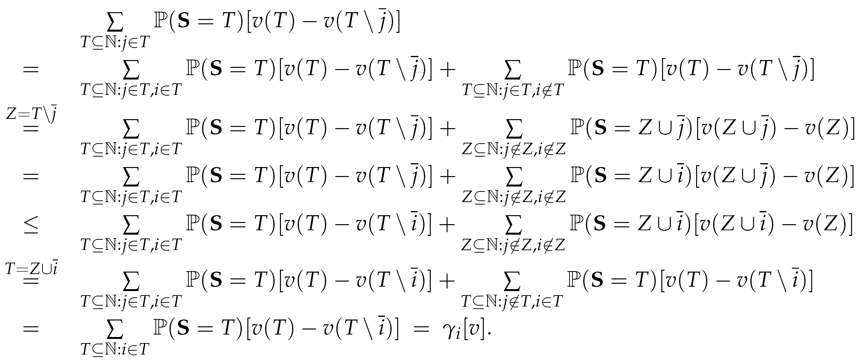
Notably, the beta-binomial distribution from Eq. (3) is not required for this result. Moreover, EEO is not necessary for all other players in , except for the condition:
This condition ensures that individuals i and j have an equal chance of being hired when both are unemployed.
Similarly, individual j’s expected marginal loss is:
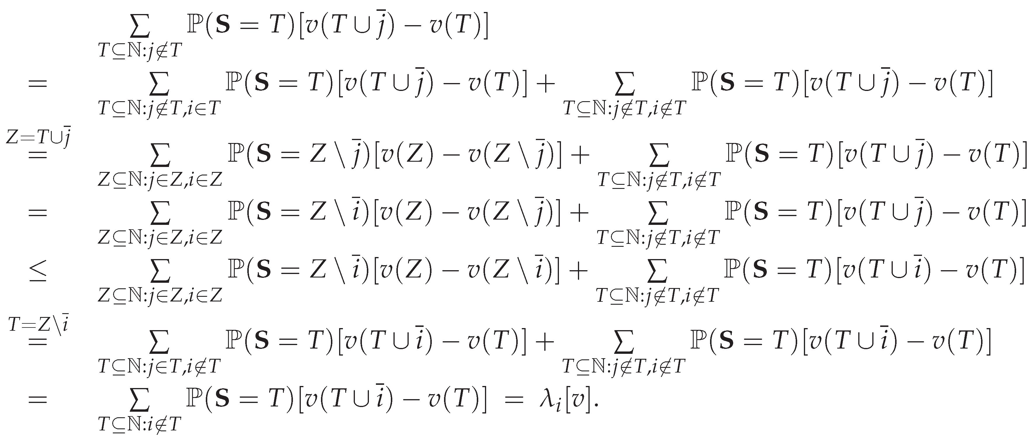
In these arguments, we use the identity:
for any subset such that . This identity ensures that individuals i and j have an equal chance of being laid off when both are employed.
Appendix I. Proof of Theorem 8
We allocate to the subset as employment welfare, and to the subset as unemployment benefits. When the employed individuals are symmetric in v and have EEO, each employed person receives:
as their employment welfare, according to Theorem 7. Similarly, when all unemployed individuals are symmetric in v and have EEO, each receives:
as their unemployment benefits.
Therefore, the condition:
is equivalent to:
Solving this equation yields:
Appendix J. Proof of Corollary 2
By Corollary 1, any -rate . Therefore, we have:
Multiplying both sides by , we obtain:
Hence, it follows that:
The remaining arguments follow directly from the proof of Theorem 8 in Appendix I.
References
- Acemoglu, D. Acemoglu, D., & Shimer, R. (2000). Productivity gains from unemployment insurance. Eur. Econ. Rev. , 44, 1195–1224. [Google Scholar] [CrossRef]
- Alm˚as, I., Hufe, P., & Weishaar, D. (2023). Equality of Opportunity: Fairness Preferences and Beliefs About Inequality. In M. Sardoˇc (Ed.), Handbook of Equality of Opportunity (pp.1–23). Springer, Cham. [CrossRef]
- Baily, M.N. Baily, M.N. (1978). Some Aspects of Optimal Unemployment Insurance. J. Public Econ, 10(3), 379–402. [CrossRef]
- Blanchard, O. (2000). The economics of unemployment: shocks, institutions, and interactions. Available online: https://economics.mit.edu/files/708 (accessed on day month year).
- Chetty, R. Chetty, R. (2006). A General Formula for the Optimal Level of Social Insurance. J. Public Econ. , 90(10-11), 1879–1901. [Google Scholar] [CrossRef]
- Devicienti, F; a note: (2010). Shapley-value decomposition of changes in wage distributions: a note. J. Econ. Inequal., 8, 35–45. [CrossRef]
- Ferrari, S. & Cribari-Neto, F. (2004). Beta Regression for Modelling Rates and Proportions. J. Appl. Stat., 7, 799–815. [CrossRef]
- Fleurbaey M., & Maniquet F. (2006). Fair income tax. Rev. Econ. Stud., 73, 55–83. [CrossRef]
- Friedman, M; a Personal Statement: , & Friedman, R. (1999). Free to Choose: a Personal Statement. Houghton Mifflin Harcourt Publishing Company, New York.
- Giorgi, G.M., & Guandalini, A. (2018). Decomposing the Bonferroni inequality index by subgroups: Shapley value and balance of inequality. Econometrics, 6, 18. [CrossRef]
- Gupta, A.K. Gupta, A.K., & Nadarajah, S. (2004). Handbook of Beta Distribution and Its Applications (Ed.). CRC Press, Boca Raton, FL.
- Hopenhayn, H.A. Hopenhayn, H.A., & Nicolini, J.P. (1997). Optimal Unemployment Insurance. J. Polit. Econ., 105(2), 412–438. [CrossRef]
- Horowitz, J.K. Horowitz, J.K., & McConnell, K. (2003). Willingness to accept, willingness to pay and the income effect. J. Econ. Behav. & Organization, 51, 537–545. [CrossRef]
- Hu, X. (2006). An asymmetric Shapley-Shubik power index. Intl. J. Game Theory, 34, 229–240. [CrossRef]
- Hu, X. (2020). A Theory of Dichotomous Valuation with Application to Variable Selection. Econometric Rev. , 39, 1075–1099. [CrossRef]
- Johnson, N.L., Kotz, S., & Balakrishnan N. (1995). Continuous Univariate Distributions, Vol. II, 2nd ed. John Wiley & Sons, New York.
- Joseph, L.B. Joseph, L.B. (1980). Some Ways of Thinking about Equality of Opportunity, Western Political Quarterly, 33(3), 393–400. [CrossRef]
- Kornhauser, M.E. (1995). Equality, liberty, and a fair income tax. Fordham Urban Law J., 23, 607–661.
- Krawczyk, P; Stat: , & Platkowski, T. (2018). Shapley value redistribution of social wealth fosters cooperation in social dilemmas. Physica A: Stat. Mech. Appl., 492, 2111–2122. [CrossRef]
- Magill, M.J.P., & Quinzii, M. (1996). Theory of Incomplete Markets, Vol. I. MIT Press, Cambridge, MA.
- Mortensen, D. T., & Pissarides, C.A. (1994). Job Creation and Job Destruction in the Theory of Unemployment. Rev. Econ. Stud., 61(3), 397–415. [CrossRef]
- Moulin, H. (2004). Fair Division and Collective Welfare, MIT Press, Cambridge, MA.
- Pissarides C.A. (1992). Loss of skill during unemployment and the persistence of employment shocks. Quart. J. Econ. , 107, 1371–1391. [CrossRef]
- Rawls, J. (1999). A Theory of Justice, 2nd ed. Harvard University Press, Cambridge, MA. Roemer, J.E. (1998). Equality of Opportunity. Harvard University Press, Cambridge, MA.
- Roemer, J.E. Roemer, J.E. (1998). Equality of Opportunity.
- Sandmo, A; a theoretical framework for justification and criticism. Swedish Econ. Policy Rev., 5, 11–33.
- Segall, S. Segall, S. (2014). Fair equality of opportunity. In J. Mandle & D.A. Reidy (Ed.), The Cambridge Rawls Lexicon (pp.269–272). Cambridge University Press. [CrossRef]
- Shapley, L.S. (1953). A value for n-person games. In H.W. Kuhn & A.W. Tucker (Ed.), Annals of Mathematics Studies, No. 28 (pp. 307–317). Princeton University Press, NJ. [CrossRef]
- Shapley, L; an outline of the descriptive theory: S. (1962). Simple games. [CrossRef]
- Tzannatos, Z. Tzannatos, Z., & Roddis, S. (1998) Unemployment benefits. World Bank Social Protection Discussion Paper Series no.9813. Washington, DC.
- Vodopivec, M. Income support for the unemployed: issues and options. World Bank Regional and Sectoral Studies no.29893. Washington, DC, 2004.
Disclaimer/Publisher’s Note: The statements, opinions and data contained in all publications are solely those of the individual author(s) and contributor(s) and not of MDPI and/or the editor(s). MDPI and/or the editor(s) disclaim responsibility for any injury to people or property resulting from any ideas, methods, instructions or products referred to in the content. |
© 2025 by the authors. Licensee MDPI, Basel, Switzerland. This article is an open access article distributed under the terms and conditions of the Creative Commons Attribution (CC BY) license (http://creativecommons.org/licenses/by/4.0/).
Copyright: This open access article is published under a Creative Commons CC BY 4.0 license, which permit the free download, distribution, and reuse, provided that the author and preprint are cited in any reuse.


