Submitted:
18 August 2025
Posted:
19 August 2025
You are already at the latest version
Abstract
The Santa Cruz Mid-County Basin Groundwater Sustainability Agency conducted a Regional Water Optimization Study (Study) to support the selection of water supply projects and management actions within the critically overdrafted Santa Cruz Mid-County Groundwater Basin (Basin), for long-term operations and shared regional benefits, including sustainable groundwater management and regional water supply needs. To support this objective, the Study utilized an integrated groundwater surface-water flow (GSFLOW) model of the Basin and surrounding areas to simulate water supply projects and management actions into the future (water year 2023 to 2075), covering the sustainability planning horizon under California’s Sustainable Groundwater Management Act (SGMA). Water supply projects and management actions considered under this study include aquifer storage and recovery (ASR), indirect potable reuse (IPR) , and interagency transfers. Many different implementations are possible for each type of project s, such that the number of potential project configurations is practically endless. To facilitate optimization, we developed a novel workflow utilizing machine learning algorithms to conduct optimization by autonomously designing, preprocessing, post-processing, and evaluating physical model scenarios. We term this workflow Machine Learning Guided Optimization (MLGO). MLGO successfully produced novel simulations and produced better performing project configurations over time.
Keywords:
groundwater
; machine learning
; modeling
; AI
; optimization
; sustainability
; seawater intrusion
; SGMA
; water resources
1. Introduction
Across the Western United States, various agencies and water providers are planning and implementing water resource sustainability projects to respond to climate change, historic overuse, and evolving supply needs. In California, Groundwater Sustainability Agencies (GSAs) must reach and maintain sustainability of their groundwater basins by 2040 in accordance with the Sustainable Groundwater Management Act (SGMA). To meet sustainability goals, GSAs are developing projects such as water reuse, managed aquifer recharge, interagency water transfers, and aquifer storage and recovery (ASR).
Effective planning of groundwater sustainability projects into the future, while accounting for climate change, typically requires using a physical groundwater flow model to simulate impacts of project configurations decades into the future. These groundwater model simulations can take hours or days to run, and adequately optimizing projects requires many iterative simulations to identify better performing project configurations. Concurrently, machine learning algorithms are increasingly being used to predict groundwater elevations and are compared favorably to physical models [1,2,3]. However, because pure ML methods are not physics-informed, and are reliant on provided training data, they may lack the generalization and predictive ability of physical groundwater models [2,4]. While studies using machine learning for optimization of physical groundwater model are extremely limited, studies in hydrology have used hybrid machine learning and physical model workflows, typically utilizing surrogate models or digital twins [5,6]. Over the past few years, studies in environmental groundwater and other fields have used machine learning for optimization of physical model simulations [7,8]. To date, optimization in the groundwater field is typically conducted manually or with the assistance of software like Model-Independent Parameter Estimation and Uncertainty Analysis (PEST).
This paper summarizes machine learning guided optimization (MLGO) implemented as part of groundwater modeling services to support the Santa Cruz Mid-County Regional Water Optimization Study (Study). The study’s objective is to support the selection of water supply projects and management actions within the critically overdrafted Santa Cruz Mid-County Groundwater Basin (Basin), for sustainable groundwater management and regional water supply needs.
2. Materials and Methods
2.1. Study Context and Area
The Mid-County Groundwater Basin occupies the middle portion of Santa Cruz County, situated in the Central Coast region of California. The Basin has a Mediterranean climate characterized by warm, mostly dry summers and mild, wet winters. Annual rainfall recorded at the Santa Cruz Co-op station within the Basin averages 29.3 inches and most rainfall occurs between November and March. California has significant climatic variability and rainfall can vary greatly from year to year. [9].
The Basin includes all areas where the stacked aquifer system of the Purisima Formation, Aromas Red Sands, and Tertiary-age aquifer units underlying the Purisima Formation constitute a shared groundwater resource managed by the Mid-County Groundwater Agency (MGA). Basin boundaries to the west are primarily geologic, defined by a granitic high. Basin boundaries to the east are primarily jurisdictional.
The Basin is dominated by the Purisima Formation which extends throughout the Basin and overlies granitic basement rock that outcrops in the west of the Basin. In the southeast of the Basin the Purisima Formation is overlain by unconfined Aromas Red Sands. The Purisima Formation is composed of named aquifer and aquitard layers, where the Aromas Red Sands is considered a single aquifer unit. Both the Purisima and Aromas aquifers are hydrologically connected to the Pacific Ocean, creating a seawater intrusion threat to the freshwater aquifers when groundwater pumping from the Basin exceeds natural and artificial groundwater recharge. Figure 1, Figure 2 and Figure 3, originally from the Mid-County Basin Groundwater Sustainability Plan, present the surficial hydrostratigraphy and the occurrence and orientation of aquifers and aquitards in the Basin [9].
MGA member agencies use a range of water supplies: Soquel Creek Water District (SqCWD) and Central Water District exclusively use groundwater, while the City of Santa Cruz primarily uses surface water including north coast streams, the San Lorenzo River, and the Loch Lomond reservoir. The City maintains a wellfield in the Basin that constitutes approximately 5% of its water supply in years with normal rainfall, but is relied upon more heavily during drought periods [9].
California’s Sustainable Groundwater Management Act (SGMA) requires the Basin to have a Groundwater Sustainability Plan (GSP) because the California Department of Water Resources (DWR) classified the Basin as high priority based on high dependence on groundwater. The Basin was also designated as as critically overdrafted due to seawater intrusion impacts on productive aquifers stemming from historical overpumping. DWR approved the MGA’s GSP [9] for the Basin in 2021, which defines groundwater sustainability via sustainable management criteria (SMC) that must be achieved by 2040 and maintained through 2070.
To support this objective, the Study utilizes an integrated groundwater surface-water numerical flow (GSFLOW) model of the Basin and surrounding areas to simulate water supply projects and management actions into the future (WY 2023 to WY2075), covering the sustainability planning horizon under the Sustainable Groundwater Management Act (SGMA). Water supply projects and management actions considered under this study include City of Santa Cruz aquifer storage and recovery (ASR), Pure Water Soquel (PWS) indirect potable reuse of recycled water via groundwater replenishment, and interagency transfers. Each project contains numerous different implementation parameters, such that the number of potential project configurations is practically endless.
The groundwater modeling aimed to identify 4 feasible and sustainable project and management action combinations that help improve regional water supply, termed ‘Alternatives’. These 4 Alternatives were then further evaluated in subsequent work products for the Study by conducting hydraulic modeling, assessing water quality compatibility, estimating financial and economic impacts, and considering environmental, social, and governance needs. Collectively, these evaluations will help project partners understand implementation feasibility and advance Basin sustainability and water supply goals.
2.2. Phyiscal Model and Water Allocation Model
Groundwater model simulations conducted to support optimization used a coupled groundwater and surface-water numerical flow (GSFLOW) model of the Santa Cruz Mid-County Basin (Mid-County) and surrounding areas which was fully calibrated for water year (WY) 1985 to WY 2015 (cite GSP), and locally recalibrated through WY 2022 to support accurate simulation of aquifer storage and recovery (ASR) testing impacts and groundwater elevations at interconnected surface water representative monitoring points (RMP)(10). This model was used to predict groundwater elevations 53 years into the future, including a climate change projection with a significantly drier and warmer climate than historical conditions (9).
Groundwater levels at RMP for 3 groundwater sustainability indicators are used to screen water supply project scenarios using groundwater modeling: seawater intrusion, depletion of interconnected surface water, and chronic lowering of groundwater levels. SMC evaluation using groundwater modeling is based on simulated groundwater elevations at RMPs. A map of RMP locations for seawater intrusion, interconnected surface water, and chronic lowering of groundwater level is shown on Figure 4 below.
To support the physical model, a Python-based water allocation or ‘transfers’ model was written to logically allocate ASR injection, ASR extraction, PWS injection, District extraction, and operational pumping changes by District supporting interagency transfers. The water allocation model is capable of accounting for these items based on highly variable project construction conditions and operational parameters. In essence, it allocates flows to utilize available surface water and meet unmet demand, based on each scenario’s unique infrastructure, project implementation, and the monthly climate timeseries. In the context of MLGO, this water allocation model serves as a pre-processor to the physical groundwater model, providing monthly timeseries injection and pumping inputs to the physical groundwater model
2.3. Machine Learning Guided Optimization Framework
To facilitate optimization of sustainability project implementation using a physical groundwater model, we developed a novel workflow of utilizing machine learning algorithms to supplement optimization by autonomously planning, preprocessing, post processing, and evaluating physical model scenarios to progress towards optimization. We term this workflow Machine Learning Guided Optimization (MLGO).
MLGO consists of a coupled, automated process where the ML algorithm learns from inputs and outputs of a physical groundwater model to conduct project optimization by automatically identifying new scenarios to simulate using results of prior model scenarios, based on user-defined optimization goals. For this project, MLGO was tasked with achieving feasibility, maintaining sustainability, and meeting projected water supply needs. To do this, it iteratively developed GSFLOW model scenarios, ran the scenarios, and post-processed results by evaluating the predictive model results until optimization goals were met. All MLGO scenarios and corresponding results were stored for the groundwater modeling team to review, utilize, and make adjustments to MLGO throughout the optimization process, based on their expertise and knowledge.
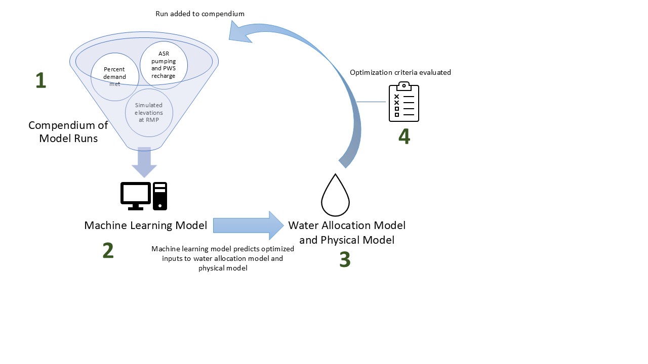
Figure 5 presents a summary of how MLGO operated by interfacing machine learning algorithms with the model. The following numbered lists refers to positions on Figure 5, which illustrate steps in the MLGO workflow.
- A set of model runs (scenarios) is constructed to form the initial compendium of scenarios for machine learning.
- a.
- The compendium contains numerical description of project parameters (physical model inputs) and evaluation criteria (physical model outputs reflecting project goals), which describe the inputs and results of each scenario.
- b.
- The initial compendium contained 5 initial scenarios created manually by the groundwater modeling team
- 2.
- A machine learning algorithm is trained on the compendium, to predict project parameters that would best meet evaluation criteria.
- a.
- Many different machine learning algorithms with different architecture were run simultaneously, with the aim of more quickly exploring the optimization parameter space and increasing the likelihood of progress towards optimization.
- b.
- Given a set of user-defined desired evaluation criteria, the machine learning algorithm suggests project parameters that are expected to meet evaluation criteria goals.
- c.
- An automated post processing script takes the MLGO suggested project parameters, and transforms them into physical model input files.
- d.
- After assembling the suggested model simulation, MLGO runs the groundwater model scenario.
- 3.
- Results from the groundwater model are post processed with respect to evaluation criteria.
- a.
- The project parameters and resulting evaluation criteria (groundwater model input and output) are then added to the compendium.
- b.
- The process then returns to step #2 and trains the machine learning algorithms on a compendium now inclusive of the new scenarios
As the compendium grows, the machine learning algorithms improve their understanding of the effect of projects on sustainability outcomes and are able to predict a different and improved set of management criteria to be run in the model. This process (steps #1 through #4) is completely automated, and can be conducted by many different agents simultaneously. Through this process, MLGO attempts to find a better set of project parameters over successive iterations.
The images on Figure 6 present an example of MLGO undergoing progressive optimization. For this example, a simple physical model analogue was constructed using a number guessing game. In this analogue, MLGO was tasked with guessing a series of 10 random numbers. The guess for each of these numbers serves as project parameters. Following each guess, a ‘scenario’ is conducted where MLGO receives the numeric distance away from each number as feedback (i.e. prediction error). This serves as an analogue for evaluation criteria output from a physical model, with the ultimate goal of having 0 distance between each number. MLGO was provided with 2 poor guesses as training data, then set to optimize for 0 prediction error. While the initial guesses are poor during an exploratory phase (iterations 1 through 10), MLGO eventually improves its guesses as it builds a repository of prior attempts during a refinement phase (iterations 10 through 40). Eventually, it explores the parameter space and optimization framework enough to guess the correct answer. This simple example illustrates the MLGO progressive learning process; over successive iterations more data is constructed by creating scenarios and running the physical model, which improves the quality of future scenarios.
2.4. Evaluation Criteria
Optimization aims to achieve an optimal or ideal situation where multiple thresholds or project goals are met. In the context of MLGO, these project goals are termed ‘Evaluation Criteria’. For this Study, evaluation criteria reflect physical model outputs that simulate feasibility and sustainability, and water allocation model outputs that account for water supply goals. An illustrative diagram summarizing the MLGO evaluation criteria is shown on Figure 7. Evaluation criteria cluster into 3 groups: sustainability, feasibility, and supply.
Sustainability: Sustainability for this project is defined based on adherence to sustainable management criteria as defined in the Basin GSP. In summary, sustainability is defined as maintaining simulated groundwater elevations above minimum thresholds (MT) at representative monitoring points (RMP). These RMP are spread across the Basin and across multiple aquifers as shown on Figure 4. Depending on the sustainability indicators each RMP is associated with, elevations may be evaluated on a monthly basis or on the basis of a 5-year moving average.
Feasibility: Feasibility for this project is defined based on maintaining daily simulated elevations below infeasible levels at ASR and PWS injection wells. A secondary aspect of feasibility is maintaining realistic pumping, quantified using seepage face losses at the ASR and production wells calculated by the MODFLOW Multi-Node Well (MNW2) package used by the GSFLOW model. Seepage flow losses result in reduced pumping due to low groundwater levels.
Supply: Supply evaluation criteria are the simplest evaluation criteria to quantify because they are already evaluated numerically based on volume of unmet supply. For this project, both cumulative unmet demand over the course of the 50-year simulation and maximum monthly unmet demand were used to quantify supply goals.
2.5. Project Parameters
In an operational optimization framework, different operational settings or model input parameters are manipulated to achieve a desired outcome. In MLGO these are referred to as ‘project parameters’ and, like evaluation criteria, must be operationalized into numbers. For this Study, project parameters reflect the myriad physical model inputs designating how projects are implemented. Evaluation criteria cluster into 3 groups, based on the associated project or management action: ASR implementation, Pure Water Soquel Implementation, and transfers implementation.
Aquifer Storage and Recovery: The ASR project parameters implemented for this study allow for up to 4 additional City ASR wells to be installed at 5 sites. The sites reflect model grid cells overlying actual available site locations. A numeric designation for layering was also implemented for model layers 7 to 9 or a combination of layers 7 and 8 or 8 and 9. At both new and existing ASR well sites, project parameters also reflected each well’s maximum pumping and injection volumes and a preferred distribution percentage amongst the wells.
Pure Water Soquel Purified Water Recharge: The PWS implementation project parameters implemented for this study allow for up to 3 additional PWS purified water injection wells to be installed at 23 sites. The sites reflect model grid cells overlying actual available site locations. A numeric designation for layering was also implemented for model layers 7 to 9 or a combination of layers 7 and 8 or 8 and 9. At both new and existing Pure Water Soquel well sites, project parameters also reflect a percentage of system-wide injection volume applied at that well and any increase in system-wide injection.
Similarly, this study also allows for up to 3 new additional SqCWD extraction wells to be installed at 23 sites. These wells extract additional water that provides in-lieu recharge uniformly across the rest of the SqCWD wellfield.
Transfers: This study allowed for bi-directional transfers between the 2 agencies: from City to District during wet periods and from District to City in dry periods. These transfers are applied using changes in pumping in the District’s production wells. Table 6 presents the project parameters reflecting transfers.
2.6. Machine Learning Algorithms
A variety of machine learning algorithms were constructed for this application of MLGO. These algorithms were deployed concurrently, with the goal of more fully exploring the optimization parameter space and ensuring generation of useful results. The algorithms used here can be grouped into 3 major categories:.
Neural network algorithms, using PyTorch [11]. Neural networks are a class of machine learning models that use layers of interconnected nodes to process data, recognize patterns, and make predictions.
Random forest algorithms, using Scikit-learn [12]. Random forests are ensemble learning methods that construct multiple decision trees during training and output a combined prediction
Combined neural network/random forest workflow algorithms, where a neural network algorithm was used for feature extraction, and a random forest algorithm was trained on the extracted features and used for prediction.
Within each category, several machine learning algorithm architectures were developed and used over the course of the project. This proved fruitful as some algorithms performed better than others, introducing variety into the compendium via different optimization pathways and potentially avoiding local minima. Examination of different algorithm success also allowed the human modelers to prioritize these better performing algorithms when allocating agents.
MLGO continuously expands its compendium of physical model scenarios as it progresses toward optimization. While a given algorithm architecture may produce a small final loss in its objective function with a relatively small dataset, over time as the dataset expands the loss function may become larger, indicating a decreased ability of the algorithm to produce meaningful scenarios using the existing architecture or hyperparameters. Therefore, the algorithm architecture and hyperparameters were periodically examined and tweaked by the supervising modeler to ensure sufficient progress.
Principal component analysis (PCA) was conducted as part of results evaluation. PCA used the PCA function from sklearn.decomposition in python.
3. Results
The MLGO workflow produced informative scenarios that anticipated how projects could be implemented sustainability and feasibility to meet regional supply needs. These scenarios included project approaches and configurations not previously envisaged by the modeling team. The process generated better solutions over time, and the large compendium of generated scenarios was useful for further examination which increasing project understanding.
3.1. MLGO Learning Over Time
The MLGO algorithm ran successfully and generated 3,407 scenarios. In Figure 9 below, each scenario is assessed for performance against a combined metric combining all of the evaluation criteria described in section 2.3 above. This metric is the sum of the normalized sustainability evaluation criteria, feasibility evaluation criteria, and supply evaluation criteria groups. Evaluation criteria groups are normalized by dividing by the max over all scenarios, exclusive of values below 5th percentile and above the 95th percentile. Figure 9 displays all runs conducted by MLGO over the analysis period, the Y axis is the combined metric representing total scenario efficacy or adherence to evaluation criteria. Lower numbers, closer to 0, represent a scenario that better meets desired goals. Runs conducted by the algorithm type that achieved the most success on average are presented in green and display an ability to improve or “learn” over time, evidenced by the reduction in the combined evaluation metric (analogous to an objective function). Though this algorithm performed best on average, it also learned from the runs conducted by all other algorithms. While a large number of scenarios was conducted, results were reviewed throughout the series of scenarios. Observations made based on scenario results were used to further constrain project parameters.
The Study organized optimization into ‘Tracks’, that specified restrictions on which projects could be expanded. Specifically, these were:
1: Planned ASR and PWS with Limited Transfers,
2: Expanded ASR,
3: Redistribute PWS (expand recharge facilities at existing recharge volumes)
4: Expand PWS (expand recharge facilities at larger recharge volumes), and
5: Expand ASR and Expand PWS (allow expanded PWS and Expanded PWS with transfers)
Accordingly, MLGO was run in ‘Tracks’, where MLGO was only allowed to manipulate certain model input information in accordance with the relevant track. In general, these tracks incorporated successive complexity by starting with the lowest amount of infrastructure expansion (and therefore smallest parameter space) and ending with the largest allowable infrastructure expansion (and therefore the largest parameter space). Incorporating successive complexity allowed MLGO to utilize its understanding of the existing parameter space, as the parameter space expanded. Examining the 50-run moving average over these tracks highlights the MLGO learning processes. At the start of each track there is typically an exploration phase where results become worse as new avenues are explored. This occurs because MLGO is testing previously unavailable options and generating data. Following this exploration phase, results begin to converge towards better solutions. This pattern is displayed on the 50-run moving average shown on Figure 9.
Results from both the exploration phase and convergence phase were informative for the modeling team to identify solutions that did and did not work. While MLGO supported analysis in all tracks, the benefit of MLGO is best exemplified by scenarios that expand ASR and expand PWS (Track 5). The overarching strategy for this track was developed first by MLGO and then refined with manual iteration. While many scenarios were conducted by using several concurrent ML algorithms running continuously, the most optimized or informative scenarios were not necessarily always produced at the end of a given track (50-run moving average approaches 0 on Figure 9). Rather, the compendium was examined continuously by staff modelers; high-performing runs were reviewed for strategic insights throughout the optimization process.
Figure 10 is an embedded video displaying the top-scoring 1,000 scenarios, visualized in a 3D space with axes of feasibility, sustainability, and supply. Gaps in the 3D optimization space illustrate the non-linearity of the solution framework: for example, injecting more purified water may improve sustainability, but make achieving feasibility more difficult. Conversely pumping more for transfers may improve supply, but decrease sustainability. Scenarios cluster along the sustainability axis; sustainability goals are highly complex and typically the most difficult to meet for both MLGO and manual optimization.
From these many scenarios, 4 Alternatives were chosen that represent highly optimized options for improving regional water supply. Two of the 4 Alternatives incorporate a strategy of symbiotically using ASR and PWS by recharging PWS near ASR facilities, that decreases the need for regional transfers. This overall strategy was derived directly from MLGO scenarios and was a new concept to the project team.
3.2. Analysis of Machine Learning Algirithms
As described above, while many agents with varying architecture and hyperparameters were utilized, the machine learning algorithm types cluster into 3 groups (random forest, neural network, and combined random forest neural network). As this study was publicly funded and therefore limited in time and scope, resources (computer core space dedicated to each algorithm type) were not allocated evenly amongst these 3 groups. Rather, priority was given to algorithm types that 1) displayed good and continuously improving adherence to evaluation criteria, and 2) displayed a perceived ability to explore the optimization parameter space by conducting novel scenarios (i.e. not repeatedly conduct the same scenario). Further, it is fully acknowledged that the manual model architecture and hyperparameter tweaking process and resource allocation conducted manually for this study heavily influenced the perceived performance of each algorithm type. Regardless, the authors feel some analysis of these 3 groups is warranted given trends observed during optimization, as each algorithm type was initially designated an equivalent amount of agent resources with similar learning metrics at the beginning of optimization.
Over most of the optimization process, random forest algorithms were given lowest prioritization for agent resource allocation. This was primarily due to a tendency to repeat the same scenarios despite a changing training dataset, and secondarily due to perceived poor optimization metrics. Acknowledging the caveats described above, this poor performance may have been due to the known challenges with using random forest to predict results outside of the training data (13; 14). Neural network algorithms were given highest priority for agent resource allocation during the middle of optimization, and second highest towards the end of optimization. This was due to their ability to generate novel scenarios with improving optimization metrics. Combined neural network/random forest algorithms were given moderate priority until the final stage of optimization, at which point they were given high priority. This was due to their apparent ability to consistently generate scenarios with good optimization metrics, especially when a larger compendium was available. While these observations are interesting conceptually, from a practical standpoint it should be noted that results from all algorithm types were printed to the same compendium, and therefore all algorithm types learned from a compendium (training dataset) that consisted of runs conducted by all algorithm types. Accordingly, it cannot be stated that a “poorly performing” algorithm type did not assist with the performance of the “high performing” algorithm type by providing useful scenarios for training.
3.3. Operational Complexity and Challenges
MLGO optimization was conducted over a period of months, during which numerical elements of the water allocation model and physical groundwater model changed substantially at several junctures. For example, during Track 2-4 optimization, MLGO began producing highly optimized scenarios that incorporated large volumes of pumping. While initially intriguing, manual review uncovered that these scenarios were exploiting features of GSFLOW that limit prescribed pumping when a well is overpumped (seepage face losses). In these circumstances the scenario results for supply and sustainability would report as very highly optimized, but this was a result of the groundwater model not reflecting the prescribed inputs. It was observed that MLGO scenarios began prioritizing the incorporation of these seepage face losses, which are essentially an error in this circumstance. Therefore, the MLGO code and framework had to be modified to record seepage face losses and to target 0 seepage face losses as an evaluation criteria. Accordingly, seepage face losses were artificially added to previously conducted runs in the compendium in accordance with new domain knowledge. Following this edit, MLGO avoided seepage face losses quite well.
Later during the optimization process, a water rights change related to dry period surface water volumes available for ASR injection was incorporated into the larger optimization framework. This substantially altered the output of the water allocation model by reducing ASR injection volumes, and therefore changed the numerical parameter space for MLGO. No modifications to the compendium or MLGO were made in this case, and MLGO continued to perform well. However, it is almost certain that having scenarios in the compendium which operated using a different water allocation model impacted MLGOs ability to predict optimized scenarios in some respect, as they constitute a form of error in the training data.
3.4. Principal Component Analysis
Analysis of high-dimensionality datasets like those generated by MLGO can be simplified through principal component analysis (PCA). PCA presents us with new simplified principal components (PCs) that efficiently organize the data to maximize variance and reveal dominant patterns in combinations of evaluation criteria and management parameter. Each evaluation criteria and management parameter contributes a percentage to each individual PC; patterns in percent contribution can elucidate trends in the compendium. Each PC can be thought of as a statistically significant trend or dominant pattern in the dataset, typically reflecting a key trade-off or relationship.
Figure 11 presents 20 PCs extracted from all scenarios conducted for this study. PCs are organized from 1 through 20 in order of cumulative increasing contribution to variance in the dataset. For example, PC1 can be used to explain just over 40% of the variability in the dataset, while PC2 contributes an additional 10%. While the dimensionality of the dataset prior to PCA is exceedingly large (58 evaluation criteria and 118 project parameters), over 60% of all variability in the compendium can be explained by the first 5 principal components. Table 7 summarizes the top 5 principal components and their relevance to the selected Alternatives. Conclusions derived from PCA support recommendations provided as part of Alternative selection as shown in Table 1.
Figure 11.
Contribution of Principal Components to Explained Variance
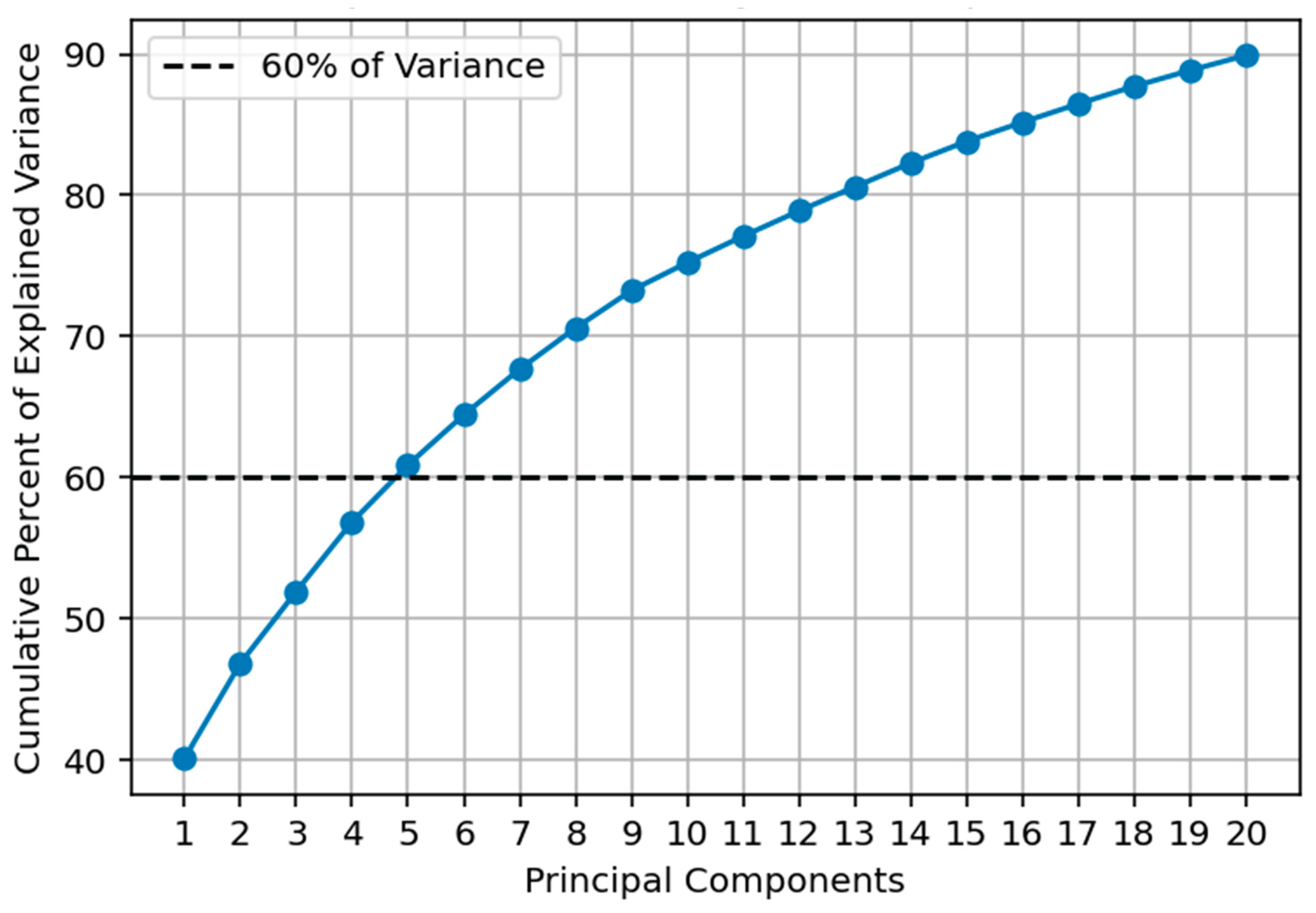

Table 3.
Summary of Top 5 Principal Components.
| Principal Component | Description | Relevance to Recommendation/Alternative |
|---|---|---|
| 1 | High volumes of District to City transfers originating from pumping near existing PWS injection wells are correlated with a lower supply gap | All 4 Alternatives prioritize utilizing District wells near existing PWS injection wells to provide water to the City during dry periods |
| 2 | Lower levels of injection at existing PWS injection wells are correlated with sustainability problems. | 3 of 4 Alternatives do not reduce injection volumes at existing PWS injection wells. Alternative 4 reduces injection at existing wells by only 6%. |
| 3 | New PWS injection wells and ASR wells which are screened solely in one aquifer are correlated with feasibility issues | Alternatives 2-4, which add ASR and/or PWS infrastructure, screen all new wells across 2 aquifers. |
| 4 | Installation of a new ASR well, PWS injection well, or PWS extraction well in a given aquifer screening is correlated with additional infrastructure expansion in that same aquifer screening | Alternatives 3-4 add pairs of ASR and PWS injection wells screened in the same aquifer. |
| 5 | Increased ASR and PWS injection and increased ASR extraction is corelated with lower transfer volumes, sustainability, increased feasibility issues at new sites, and decreased feasibility issues at existing sites | 3 of 4 Alternatives include some infrastructure expansion which reduces the need for District to City District transfers |
4. Discussion
Overall, MLGO was an effective method for optimizing this complex system. Not only did MLGO progress towards optimization over time and produce scenarios with increasingly improved optimization metrics, it also generated a large compendium of scenarios that proved useful for selecting final design Alternatives and increasing project understanding. Additional principal component analysis helped identify generalized principals which could be used to guide practical implementation of projects. Ultimately, the machine learning algorithms used here, and therefore the MLGO process, are heuristic in nature. The machine learning agents attempt to solve the entire optimization problem presented to them at once, and therefore attempt to progress by the shortest path possible to the desired result. In theory, this allows for rapid efficient optimization in a practical applied setting, as time is not spent methodically perturbing project parameters or intentionally randomly sampling the project parameter space. However, this also raises the possibility that an alterative solution may be missed during the MLGO process, that might have been captured by software that more systematically perturbs parameters to conduct scenarios. This risk was reduced by introducing manual scenarios into the initial training data that explored various strategies and by having multiple ML algorithms that explored the parameter space in different ways.
Metalearining or meta learning refers to an AI algorithm ‘learning to learn’ [15]. Rather than the non-meta learning that takes place when an algorithm trains itself on a static dataset, metalearning encompasses changes to algorithm structure or hyperparameters that allow it to adapt to a changing dataset or optimization framework. Some sort of manual or automated architecture or hyperparameter adjustment is critical for MLGO, as it is continuously expanding its dataset of model scenarios as it progresses towards optimization. While a given algorithm architecture may produce small final loss in its objective function with a relatively small dataset, over time as the dataset expands, the loss function may become larger indicating a decreased ability of the algorithm to produce meaningful scenarios using the existing architecture or hyperparameters. Therefore, the algorithm architecture and hyperparameters must be periodically examined and tweaked by the automated workflow itself (self-imposed metalearning or true metalearning), or by the supervising modeler (user-imposed metalearning/modification). For this study, this modification was largely user-imposed as described in the methods. While MLGO progressed autonomously, metrics for total objective function loss during the learning process were recorded and analyzed by the overseeing modeler. If loss was judged to be stagnating or getting larger over time as the dataset expands, the modeler would make tweaks to hyperparameters or model architecture until it produced low levels of loss. Future work with MLGO could lessen its reliance on manual manipulation of architecture or hyperparameters by incorporating automated ML algorithm optimization. True self-imposed metalearning could be implemented by building functionalities that test a range of hyperparameters and architectures, and then selecting a ‘Best Algorithm’ from these (15). As highlighted in the results, the overall success of a given algorithm in producing high-quality scenarios is highly dependent on the architecture and hyperparameters of that algorithm, and the skill of the manual machine learning engineer in manually adjusting these elements. By utilizing true metalearning, high-quality scenarios could be generated more consistently with less manual intervention, theoretically reducing the number of scenarios required to reach sufficient optimization.
During development and presentation of MLGO, comparisons were often made to Model-Independent Parameter Estimation and Uncertainty Analysis (PEST), an industry-standard software frequently used for calibration of numerical models, particularly groundwater flow models. PEST undertakes highly parameterized inversion of environmental models. In doing so, it runs a model many times, either sequentially or in parallel [16]. MLGO differs from PEST mainly in that it does not conduct inversion or explicitly conduct runs perturbing the parameter space to create a Jacobian matrix. Rather, it learns from an ever-growing compendium of scenario data and relies on the internal mechanisms of the machine learning algorithms to generate a fit to the data. This process can be stopped and restarted at any time without loss of data, and the compendium can be manipulated without interruption of the process. Rather than iteratively perturbing parameters, and MLGO immediately attempts to solve the problem heuristically at any given point. In theory, given a set of well-trained machine learning algorithms, this could result in a faster time to optimization relative to PEST, however no such comparison is attempted here. Future work could compare the time to optimization for both MLGO and PEST, though each process will be highly dependent on its implementation and therefore direct comparison may be difficult. In future applications, it could also be possible to leverage both PEST and MLGO; MLGO could operate in conjunction with PEST by gathering additional compendium scenarios from those conducted by a concurrent PEST run. In this way, MLGO would learn from PEST, which methodically perturbs parameters, while simultaneously continuing its heuristic optimization.
As described above, early in optimization MLGO observed seepage face losses (in this circumstance essentially a physical model software bug) and heuristically prioritized these scenarios before a manual intervention to edit the optimization framework. An advantage of MLGO is that the compendium of previous runs can be manually edited to reflect changes in the optimization framework, which was done here to flag scenarios with this bug. As each MLGO agent conducts deep learning on the compendium ‘from scratch’ to conduct each scenario, it was relatively straightforward to incorporate a change in the optimization framework and preserve compendium data where possible. This flexibility may be an advantage when compared to other optimization software.
Optimization for this project was conducted using a single deterministic projected scenario. Future applications of MLGO could use an objective function that optimizes project implementation over many scenarios. Workflows similar to MLGO may also be used for calibration and parameter estimation. Finally, optimization of projects with fixed infrastructure could use MLGO with reinforcement learning algorithms to make implementation decisions and evaluate project efficacy at each numerical model timestep.
Author Contributions
Conceptualization, P.W., C.T., and T.B.; methodology, P.W; validation, P.W and C.T.; formal analysis, P.W, C.T., and T.B.; writing—original draft preparation, P.W.; writing—review and editing, C.T, T.B..; visualization, P.W., C.T.; project administration, C.T. All authors have read and agreed to the published version of the manuscript.
Funding
This research was funded by Mid-County Groundwater Agency through a California Department of Water Resources Prop 1 grant.
Data Availability Statement
No new data were created or analyzed in this study. Data sharing is not applicable to this article.
Acknowledgments
This work was supported by funding and staff from Soquel Creek Water District and the City of Santa Cruz Water Department. Special thanks to, Shelley Flock, Heidi Luckenbach, and Melanie Mow Shumacher.
Conflicts of Interest
The authors declare no conflicts of interest.
Abbreviations
The following abbreviations are used in this manuscript:
| ASR | Aquifer Storage and Recovery |
| PWS | Pure Water Soquel |
| MLGO | Machine Learning Guided Optimization |
| GSFLOW | Groundwater Surface Water Flow Model |
| ML | Machine Learning |
| PCA | principal component analysis |
| RF | Random Forest |
| NN | Neural Network |
| SGMA | Sustainable Groundwater Management Act |
| WY | Water Year |
References
- Malekzadeh, M.; Kardar, S.; Shabanlou, S. Simulation of groundwater level using MODFLOW, extreme learning machine and Wavelet-Extreme Learning Machine models. Groundw. Sustain. Dev. 2019, 9. [Google Scholar] [CrossRef]
- Chen, C.; He, W.; Zhou, H.; Xue, Y.; Zhu, M. A comparative study among machine learning and numerical models for simulating groundwater dynamics in the Heihe River Basin, northwestern China. Sci. Rep. 2020, 10, 1–13. [Google Scholar] [CrossRef] [PubMed]
- Tao, H.; Hameed, M.M.; Marhoon, H.A.; Zounemat-Kermani, M.; Heddam, S.; Kim, S.; Sulaiman, S.O.; Tan, M.L.; Sa’aDi, Z.; Mehr, A.D.; et al. Groundwater level prediction using machine learning models: A comprehensive review. Neurocomputing 2022, 489, 271–308. [Google Scholar] [CrossRef]
- Asher, M.J.; Croke, B.F.W.; Jakeman, A.J.; Peeters, L.J.M. A review of surrogate models and their application to groundwater modeling. Water Resour. Res. 2015, 51, 5957–5973. [Google Scholar] [CrossRef]
- Dai, T.; Maher, K.; Perzan, Z. Machine learning surrogates for efficient hydrologic modeling: Insights from stochastic simulations of managed aquifer recharge. J. Hydrol. 2025, 652. [Google Scholar] [CrossRef]
- Marshall, S.R.; Tran, T.-N.; Tapas, M.R.; Nguyen, B.Q. Integrating artificial intelligence and machine learning in hydrological modeling for sustainable resource management. Int. J. River Basin Manag. 2025, 1–17. [Google Scholar] [CrossRef]
- Fang, Z.; Ke, H.; Ma, Y.; Zhao, S.; Zhou, R.; Ma, Z.; Liu, Z. Design optimization of groundwater circulation well based on numerical simulation and machine learning. Sci. Rep. 2024, 14, 1–14. [Google Scholar] [CrossRef] [PubMed]
- Wu, F.; Yang, X.; Ma, Y.; Zhang, Q.; Zhang, Z.; Yuan, X.; Liu, H.; Liu, Z.; Zhong, J.; Zheng, J.; et al. Machine-learning guided optimization of laser pulses for direct-drive implosions. High Power Laser Sci. Eng. 2022, 1–10. [Google Scholar] [CrossRef]
- Mid-County Groundwater Management Agency (MGA). (2019). Santa Cruz Mid-County Groundwater Basin Groundwater Sustainability Plan, Midhttps://www.midcountygroundwater.org/sites/default/files/uploads/MGA_Draft_GSP_Cover_Acknowledgments_Abbv_7-12-2019.
- Montgomery & Associates (M&A). (2024). Santa Cruz Mid-County Basin Optimization Study, Summary of Groundwater Modeling Supporting Alternative Selection (Technical Memorandum 3). Montgomery & Associates: Tucson, AZ, USA.
- Ansel, J., Yang, E., He, H., Gimelshein, N., Jain, A., Voznesensky, M., Bao, B., Bell, P., Berard, D., Burovski, E., et al. (2024). PyTorch 2: Faster Machine Learning Through Dynamic Python Bytecode Transformation and Graph Compilation. In Proceedings of the 29th ACM International Conference on Architectural Support for Programming Languages and Operating Systems (ASPLOS '24), San Diego, CA, USA, 27 April–1 May 2024; Volume 2. [CrossRef]
- Pedregosa, F., Varoquaux, G., Gramfort, A., Michel, V., Thirion, B., Grisel, O., ... & Duchesnay, E. (2011). Scikit-learn: Machine Learning in Python. Journal of Machine Learning Research, 12, 2825–2830. Available online: https://jmlr.csail.mit.edu/papers/v12/pedregosa11a.html.
- Hengl, T.; Nussbaum, M.; Wright, M.N.; Heuvelink, G.B.M.; Gräler, B. Random forest as a generic framework for predictive modeling of spatial and spatio-temporal variables. PeerJ 2018, 6, e5518. [Google Scholar] [CrossRef] [PubMed]
- Wang, Y., & King, R. D. (2023). Extrapolation is not the same as interpolation. In Discovery Science, DS 2023, Bifet, A., Lorena, A. C., Ribeiro, R. P., Gama, J., & Abreu, P. H. (Eds.), Lecture Notes in Computer Science, Springer: Cham, Switzerland, Volume 14276, pp. 276–289. [CrossRef]
- Brazdil, P., Giraud-Carrier, C., Soares, C., & Vilalta, R. (2022). Metalearning: Applications to Automated Machine Learning and Data Mining. Springer Nature: Cham, Switzerland.
- White, J., Welter, D., & Doherty, J. (2019). PEST++ Version 4.2.1 Documentation. U.S. Department of the Interior, Bureau of Reclamation: Denver, CO, USA.
Figure 1.
Hydrostratigraphic Outcrops in Mid-County Basin [Mid-County Basin Groundwater Sustainability Plan].
Figure 1.
Hydrostratigraphic Outcrops in Mid-County Basin [Mid-County Basin Groundwater Sustainability Plan].
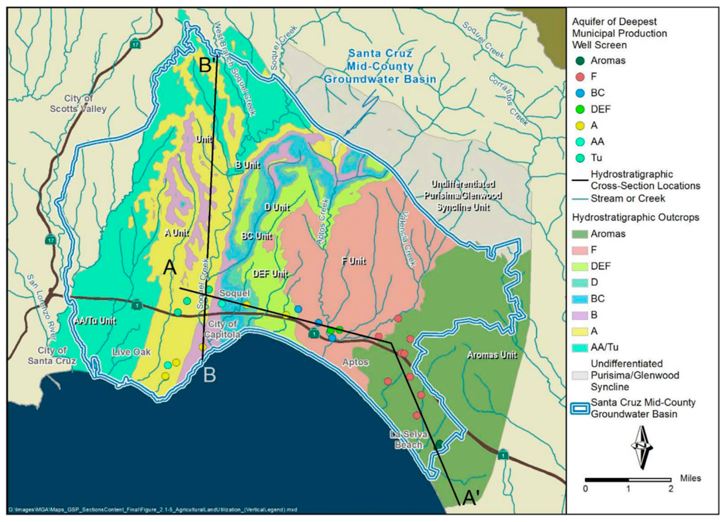
Figure 2.
Hydrostratigraphic Cross Section A-A’ in Mid-County Basin [Mid-County Basin Groundwater Sustainability Plan].
Figure 2.
Hydrostratigraphic Cross Section A-A’ in Mid-County Basin [Mid-County Basin Groundwater Sustainability Plan].
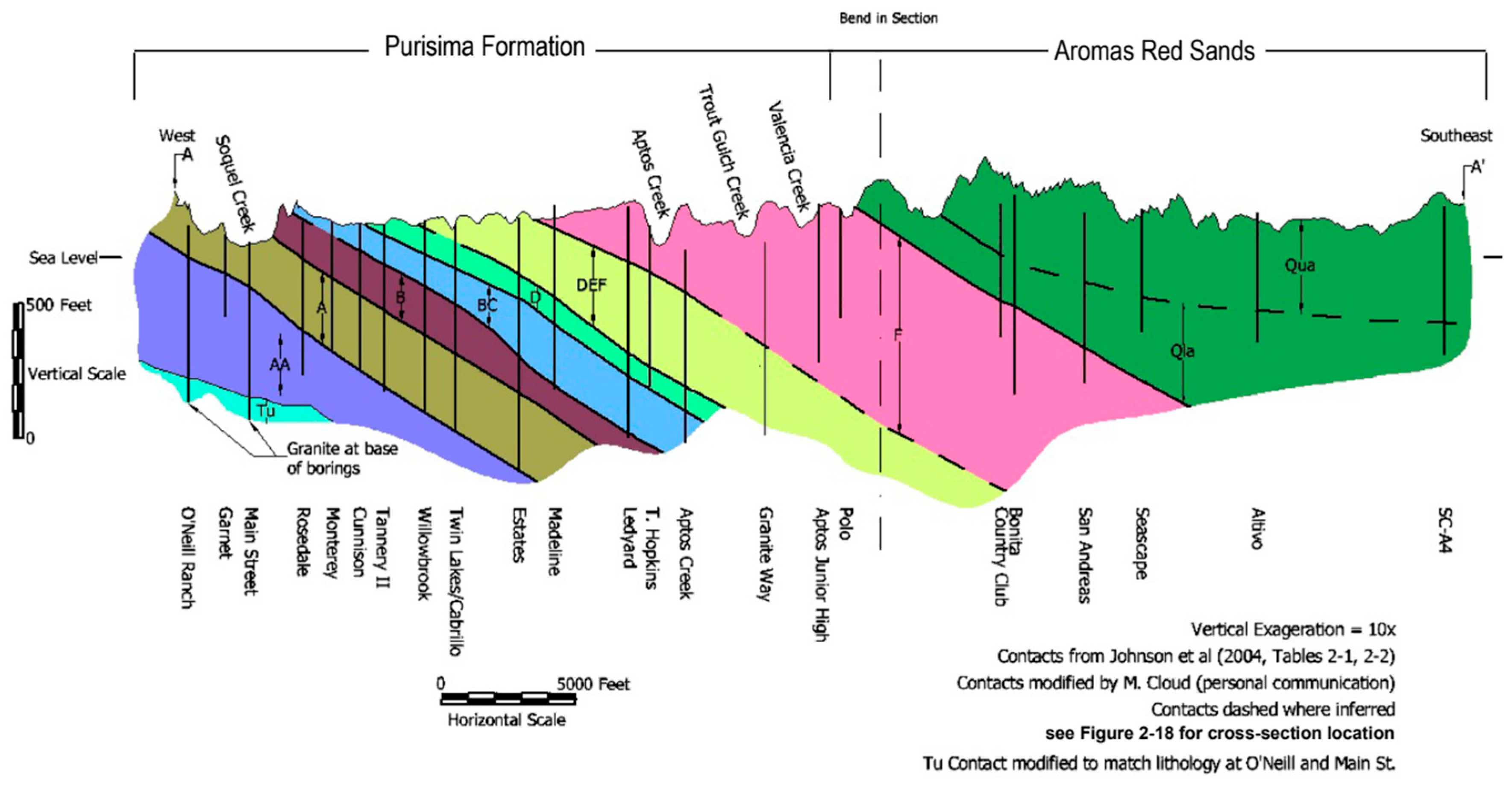
Figure 3.
Hydrostratigraphic Cross Section B-B’ in Mid-County Basin [Mid-County Basin Groundwater Sustainability Plan].
Figure 3.
Hydrostratigraphic Cross Section B-B’ in Mid-County Basin [Mid-County Basin Groundwater Sustainability Plan].
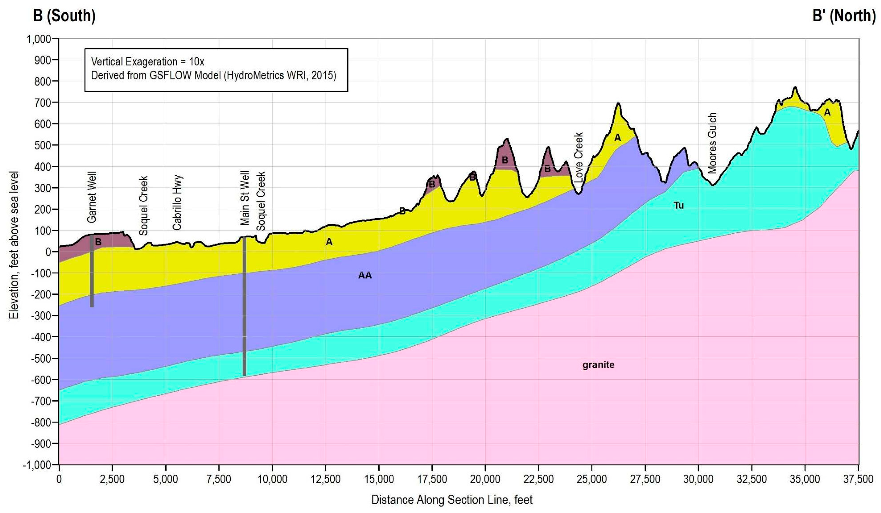
Figure 4.
Representative Monitoring Points by Sustainability Indicator.
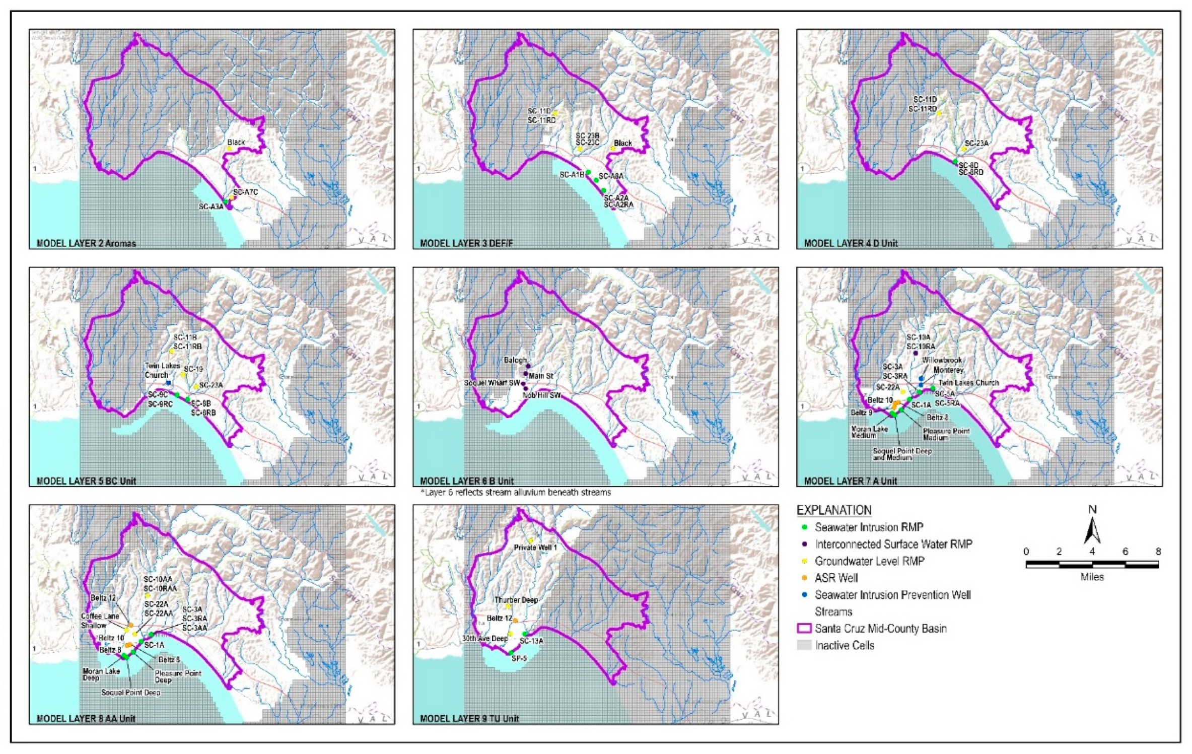
Figure 5.
Machine Learning Guided Optimization Overview.
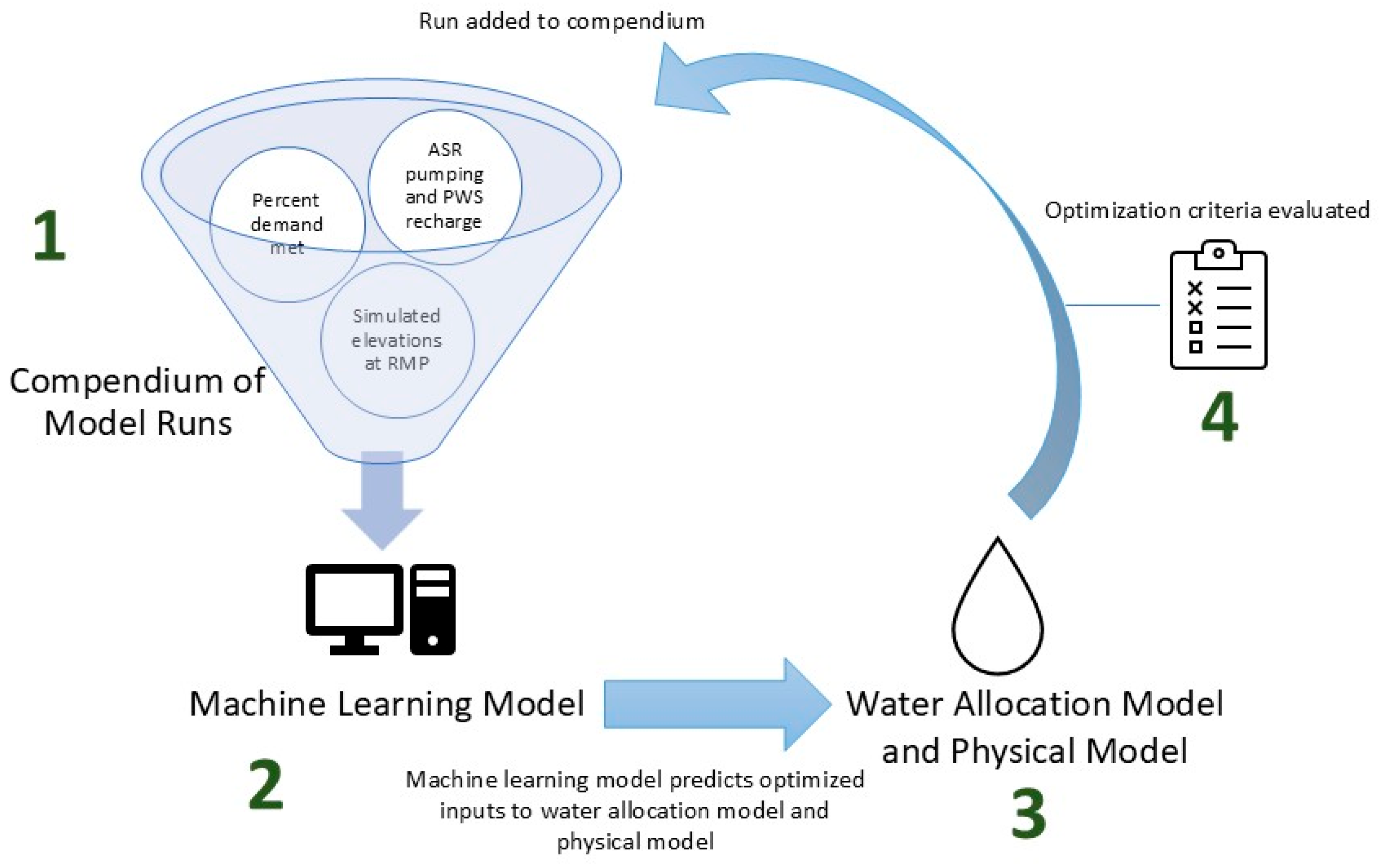
Figure 6.
Simple Example of MLGO In Real Time.
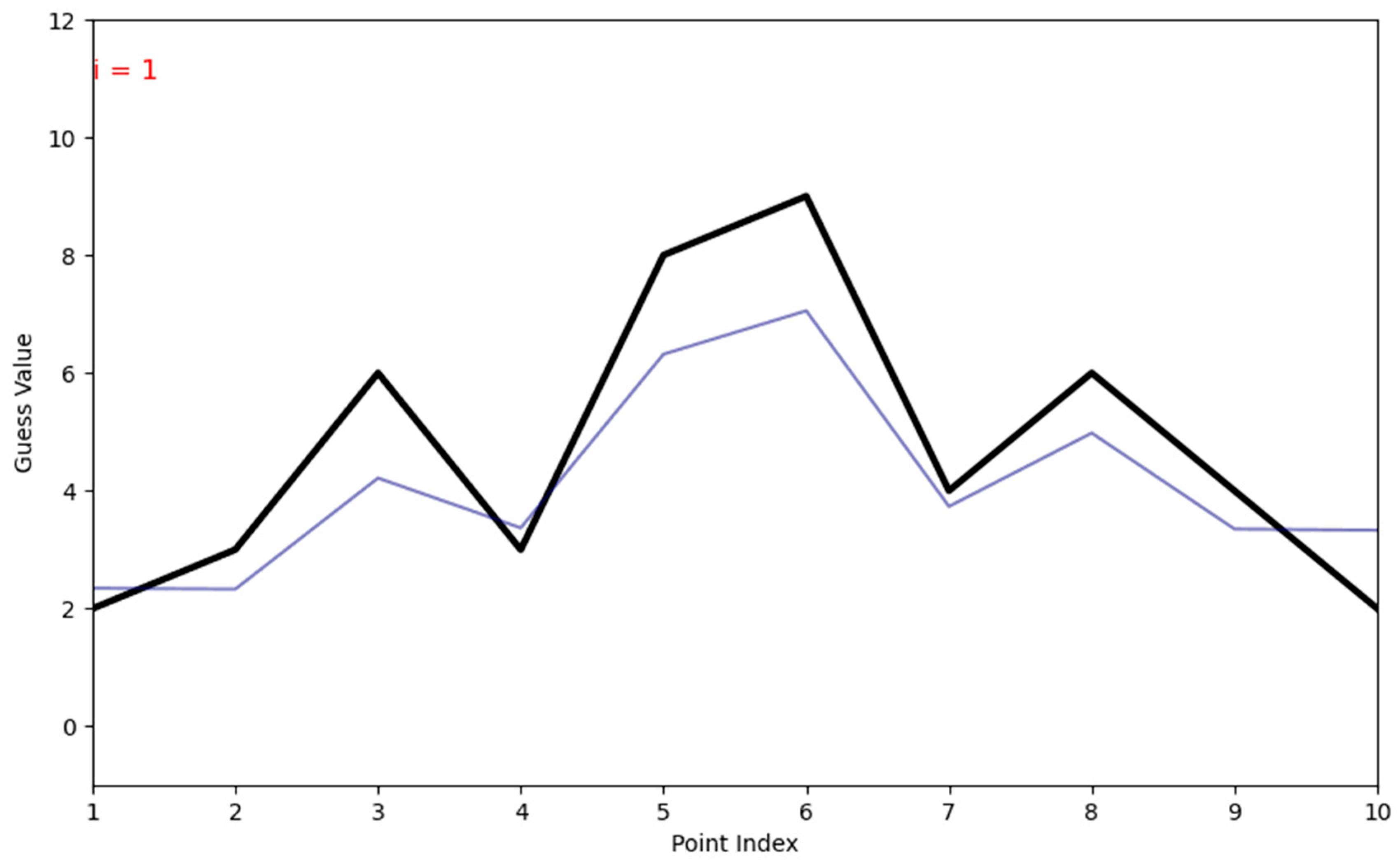
Figure 7.
Summary of Evaluation Criteria.
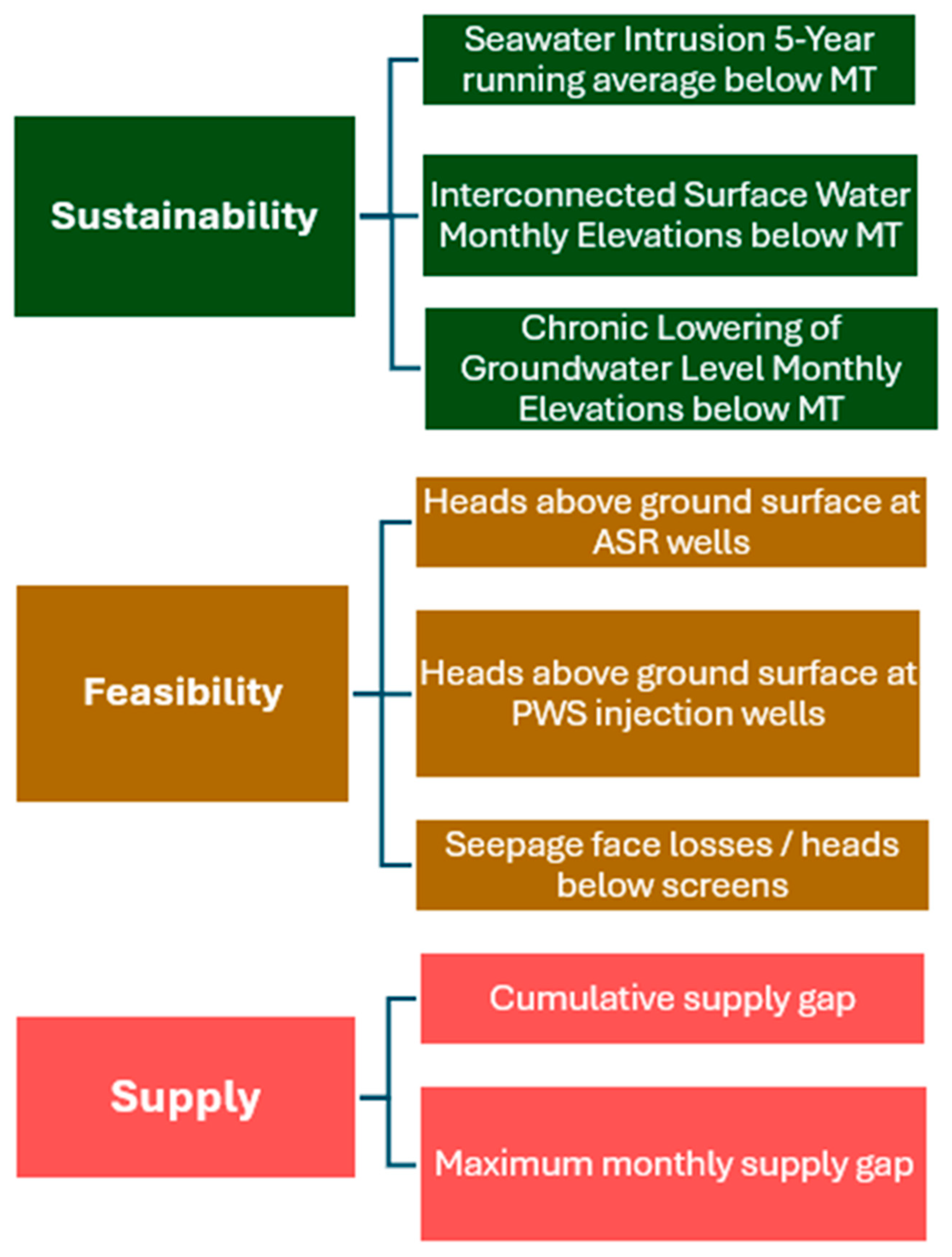
Figure 8.
Summary of Project Parameters.
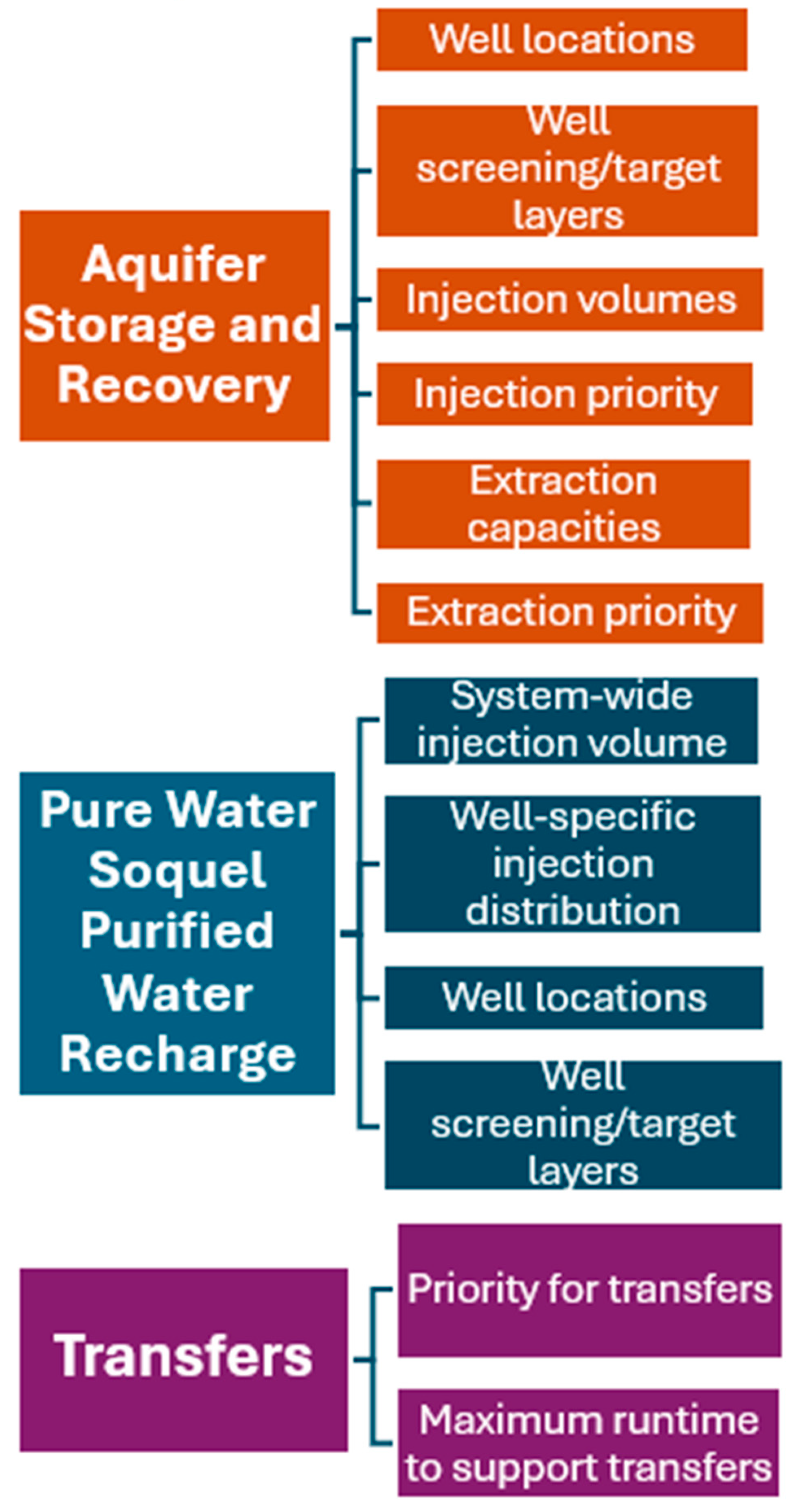
Figure 9.
MLGO Scenario Performance Over Time.
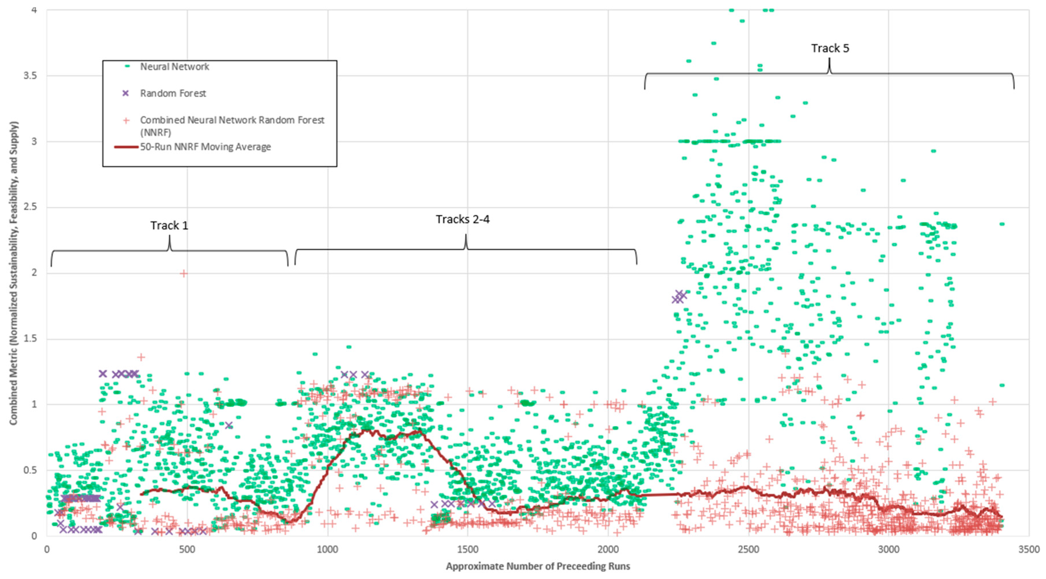
Figure 10.
Video: 3D Visualization of Top 1,000 Scenarios [Digital Animation].
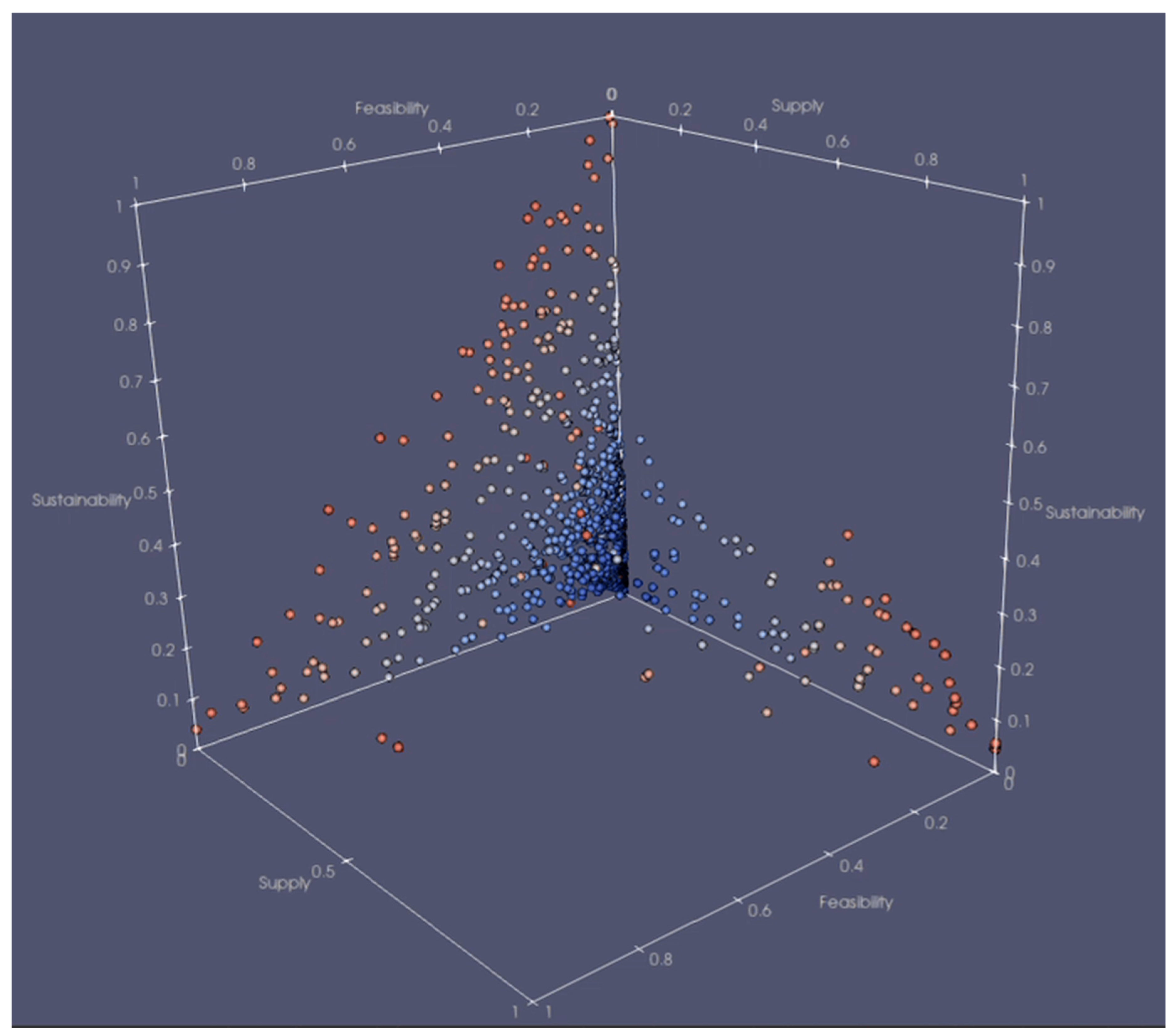
Table 1.
Summary of Evaluation Criteria.
| Group | Evaluation Criteria | Operationalization and Description |
|---|---|---|
| Sustainability | Seawater Intrusion | Cumulative 5-year running average head below MT at seawater intrusion RMP |
| Depletion of Interconnected Surface Water | Cumulative monthly head below MT at interconnected surface water RMP | |
| Chronic Lowering of Groundwater Level | Cumulative monthly head below MT at interconnected surface water RMP | |
| Feasibility | ASR injection elevations | Cumulative head above infeasible elevations (0 or 10 feet above ground surface depending on location) |
| ASR seepage face losses | Cumulative number of days when simulated seepage face losses occur | |
| Pure Water Soquel injection elevations | Cumulative head above infeasible elevations (0 feet above ground surface) | |
| Supply | Cumulative supply gap | Cumulative supply gap that occurs across the projected scenario |
| Maximum monthly supply gap | Maximum monthly supply gap that occurs across the projected scenario |
Table 2.
Summary of Project Parameters.
| Group | Parameter | Description | Minimum | Maximum |
|---|---|---|---|---|
| ASR | Site location for new ASR wells | ASR sites are numbered 1-5 as shown on Figure 13 | 1 (Site 1) | 5 (Site 5) |
| Layering for new ASR wells | Layering reflects model layers 7-9, and combinations of layers 7/8 and layers 9/10. | 7 (Layer 7, Purisima A) | 11 (Layer 8 and Layer 9 Purisima AA and Tu) | |
| Injection and extraction weights for existing and new ASR wells | Weights are used to develop a desired relative injection or extraction percentage, for the water allocation model | 0 (no injection/ extraction) | 50 (maximum weight for injection/ extraction) | |
| Injection and extraction maximum runtimes | Determines the maximum injection or extraction capacity | 1 (predicted sustainable and feasible capacity informed by previous work) | 5 (aspirational capacity identified by City staff) | |
| O’Neill as ASR | Binary check for whether the District O’Neill production well should be operated as an ASR well or exclusively as a District production well | 0 (District production well) | 1 (ASR well) | |
| Pure Water Soquel (injection wells) | Site location for new PWS injection wells | PWS sites are numbered 1-23 as shown on Figure 13 | 1 (Site 1) | 23 (Site 23) |
| Layering for new PWS injection | Layering reflects model layers 7-9, and combinations of layers 7/8 and layers 8/9 | 7 (Layer 7, Purisima A) | 11 (Layer 8 and Layer 9 Purisima AA and Tu) | |
| Injection weights for new and existing PWS injection wells | Weights are used to develop a desired relative injection percentage, for the water allocation model | 0 (no injection/ extraction) | 50 (maximum weight for injection/ extraction) | |
| Pure Water Soquel (new District extraction wells) | Added PWS injection volume | Additional volumes of injection, in addition to planned 1,500 AFY | 0 (no added injection) | 7 (additional injection of 1,500 AFY) |
| Site location for new SqCWD extraction wells | Sites are numbered 1-23 as shown on Figure 13 | 1 (Site 1) | 23 (Site 23) | |
| Layering for new SqCWD extraction | Layering reflects model layers 7-9, and combinations of layers 7/8 and layers 8/9. | 7 (Layer 7, Purisima A) | 11 (Layer 8 and Layer 9 Purisima AA and Tu) | |
| Extraction weights for new PWS extraction wells | Weights are used to develop a desired relative extraction percentage, for the water allocation model | 0 (no extraction) | 50 (maximum weight for extraction) | |
| Added PWS extraction volume | Additional volumes of extraction applied at new PWS extraction wells | 0 (no added extraction) | 7 (additional extraction of 1,500 AFY) | |
| Transfers | Transfers priorities for District to City transfers | The order in which pumping is increased to support District to City transfers across the District’s production wells | 1 (1st in order) | 19 (last in order) or 20 (no increases allowed) |
| Max runtimes for transfers | Maximum runtimes allowed for wells supporting transfers from District to City | 1 (12 hours per day) | 5 (21.6 hours per day) | |
| Reduction priorities for City to District transfers | The order in which pumping is decreased to support City to District transfers across the District’s production wells | 1 (1st in order) | 19 (last in order) or 20 (no decreases allowed) | |
| Limit transfers | Binary check for whether transfers are limited to existing intertie capacity or unlimited | 0 (transfers limited) | 1 (transfers not limited) |
Disclaimer/Publisher’s Note: The statements, opinions and data contained in all publications are solely those of the individual author(s) and contributor(s) and not of MDPI and/or the editor(s). MDPI and/or the editor(s) disclaim responsibility for any injury to people or property resulting from any ideas, methods, instructions or products referred to in the content. |
© 2025 by the authors. Licensee MDPI, Basel, Switzerland. This article is an open access article distributed under the terms and conditions of the Creative Commons Attribution (CC BY) license (http://creativecommons.org/licenses/by/4.0/).
Copyright: This open access article is published under a Creative Commons CC BY 4.0 license, which permit the free download, distribution, and reuse, provided that the author and preprint are cited in any reuse.


