Submitted:
15 August 2025
Posted:
18 August 2025
You are already at the latest version
Abstract
To address the challenge of effectively filtering out noise components in GNSS coordinate time series, we propose a denoising method based on parameter-optimized Variational Mode Decomposition (VMD). The method combines permutation entropy with mutual information as the fitness function, and uses the crayfish (COA) algorithm to adaptively obtain the optimal parameter combination of the number of modal decompositions and quadratic penalty factors for VMD. employs permutation entropy combined with mutual information as the fitness function and utilizes the Crayfish Optimization Algorithm (COA) to adaptively determine the optimal parameter combination for VMD, including the number of decomposition modes and the quadratic penalty factor. The GNSS coordinate time series is decomposed into several intrinsic mode function (IMF) components, and sample entropy is used to identify the effective modal components, which are then reconstructed into the denoised signal, achieving effective separation of signal and noise. The experiments were conducted using simulated signals and 52 raw GNSS measurement data from CMONOC to compare and analyze the COA-VMPE-WD method with wavelet denoising (WD), empirical mode decomposition (EMD), ensemble empirical mode decomposition (EEMD), and Complete Ensemble Empirical Mode Decomposition with Adaptive Noise (CEEMDAN) methods. The result shows that the COA-VMPE-WD method can effectively remove noise from GNSS coordinate time series and preserve the original features of the signal, with the most significant effect on the U component, the COA-VMPE-WD method reduced station velocity by an average of 50.00%, 59.09%, 18.18%, and 64.00% compared to the WD, EMD, EEMD, and CEEMDAN methods, The noise reduction effect is higher than the other four methods, providing reliable data for subsequent analysis and processing.
Keywords:
GNSS
; optimization algorithm for crayfish
; variational mode decomposition
; permutation entropy
; wavelet decomposition
; signal denoising
1. Introduction
Due to factors such as the external environment of the monitoring station, unmodeled errors, and geophysical effects, Global Navigation Satellite System (GNSS) coordinate time series exhibit significant nonlinear variations, containing various signals [1] and colored noise [2,3]. The noise components in GNSS coordinate time series are complex, affecting the estimation of station velocity and its uncertainty, and even leading to misinterpretations of certain geophysical phenomena [4,5]. Therefore, in the analysis of GNSS coordinate time series, effectively reducing the impact of noise to obtain accurate station velocity and its uncertainty is of great significance for establishing high-precision velocity field models [6,7,8,9] and analyzing geophysical phenomena such as plate tectonic movements [10,11].Studies have shown that common methods for denoising GNSS coordinate time series [3,4,12,13,14] include wavelet analysis [15,16], singular spectrum analysis (SSA) [17,18], empirical mode decomposition (EMD), ensemble empirical mode decomposition(EEMD) and complete ensemble empirical mode decomposition with adaptive noise (CEEMDAN) et al. [19,20]. Kunpu and Yunzhong S. (2020) proposed a non-interpolated wavelet analysis algorithm that effectively extracts seasonal signals from GNSS coordinate time series [21]. However, in wavelet analysis, the selection of basis functions and decomposition levels lacks adaptability, and different basis functions and decomposition levels can significantly impact the denoising performance of the algorithm. Dong et al. (2002) employed wavelet decomposition (WD) and SSA to model the nonlinear variations in GNSS coordinate time series, reducing the likelihood of useful signals being mistakenly filtered out as noise [22]. Nevertheless, SSA analysis involves subjectivity in selecting the lag window, and different window lengths greatly affect the signal extraction results. Liu et al. (2023) used EMD to correct the periodic terms in GNSS continuous station time series, obtaining relatively reliable station velocities [23]. However, EMD is prone to endpoint effects and mode mixing. To mitigate this phenomenon, Yeh et al. (2010) proposed an optimized version of EMD called ensemble empirical mode decomposition (EEMD) [24], and Agnieszka and Dawid (2022) supplemented the ensemble EMD algorithm. However, both algorithms suffer from low computational efficiency [25], and their decomposition performance heavily depends on the number of ensemble trials and the amplitude of the added white noise.
Dragomiretskiy and Zosso (2013) proposed a non-recursive signal decomposition method called variational mode decomposition (VMD) [26]. Unlike EMD, which iteratively sifts and peels off signals [27], VMD essentially constructs and solves a variational problem, effectively avoiding the mode mixing and endpoint effects inherent in EMD. VMD possesses adaptive characteristics and circumvents the issues associated with EMD while also exhibiting advantages in noise robustness. As a result, VMD has been widely applied in signal denoising research [28,29,30]. However, VMD requires the predefinition of two critical parameters that influence its decomposition performance: the number of modes () and the penalty factor (). In practical applications, and are often selected empirically, and inappropriate parameter choices can lead to over-decomposition or under-decomposition of the signal, adversely affecting denoising results [31]. Lu and Xie (2021) introduced a comprehensive index T to determine the optimal value for VMD denoising [32]. This method fixes the value and only considers the impact of on the denoising performance of the VMD algorithm, neglecting the interplay between and , and thus can only yield a relatively suboptimal parameter combination.
Based on the above, in this study, we propose a novel denoising method (COA-VMPE-WD) that combines Variational Mode Decomposition (VMD) optimized by the Crayfish Optimization Algorithm (COA) using envelope entropy as the fitness function, with multiscale permutation entropy (MPE) as a constraint condition (COA-VMPE), and wavelet decomposition (WD). This method is applied to denoise GNSS coordinate time series, and its effectiveness and reliability are validated through experiments on simulated signals and real GNSS observation data. The root means square error (RMSE), signal-to-noise ratio (SNR), mean absolute error (MAE), and cross-correlation coefficient (R) as the denoising evaluation indicators.
The organization of the work is as follows: Section 2 describes the GNSS data and mathematical methods. Section 3 shows the parameters of COA optimized VMD, optimal parameters selection, results of different denoising methods between simulated signals and real GNSS. Section 4 discusses the COA-VMPE-WD method and existing noise reduction methods for detecting the optimal noise model and analyzing the impact of GNSS station annual term and station velocity. Section 5 concludes this work.
2. Data and Methods
2.1. Data
In this study, to further verify the reliability and applicability of the COA-VMPE-WD method, we selected the original coordinate time series of 52 GNSS reference station networks in China for research and analysis. The observation time was GNSS coordinate time series data from 2010 to 2023, sourced from Crustal Movement Observation Network of China (CMONOC).The data we have selected meets the following conditions: 1) Data missing less than 10%; 2) The missing data is filled in by using the single spectrum analysis (SSA) method to fill in the differences; 3) We used the 3 interquartile range (3IQR) method for coarse error removal. The distribution of selected sites in the study is shown in Figure 1.
2.2. Methods
2.2.1. Crayfish Optimization Algorithm
Crayfish Optimization Algorithm (COA) is a metaheuristic algorithm inspired by the foraging and enemy avoidance behavior of crayfish COA has the ability to efficiently balance global exploration and local development [33]. It simulates the temperature convergence, foraging competition, and cave avoidance behavior of crayfish, and dynamically balances global exploration (moving away from the current optimal solution) and local development (finely searching nearby areas) through temperature factors (controlling individual movement range) and random disturbance strategies, avoiding premature convergence. As the iteration progresses, the algorithm automatically reduces the search range (similar to a cooling process), gradually shifting from extensive exploration to local optimization, and improving convergence accuracy.
The implementation of COA algorithm mainly consists of six steps [34]:
Step 1: Parameter definition and initialization of population
We define T is the number of iterations, N is population, dim is dimension, ub is upper bound, lb is lower bound, X is initializing population based on upper and lower bounds (formula1). Xi,j is the position of individual i in the j dimension, and Xi,j value is obtained from formula (1). and rand is a random number of Ezugwu et al. (2021) [35].
Step 2: Define temperature
The ambient temperature of crayfish is defined according to formula (3) to make COA enter different stages. We determine the temperature(temp) and intake of crayfish p [36], as shown in formula (3) .
µ is the temperature most suitable for crayfish, σ and C1 are used to control the intake of crayfish at different temperatures.
Step 3: Summer resort stage and competition stage
When the temperature is above 30 (temp>30°), the temperature is too high, crayfish will choose to spend their summer vacation in caves. The definition of Xshade cave is as follows [34]:
XG is the optimal position obtained so far by the number of iterations, and XL is the optimal position of the current population. When rand<0.5, crawfish will directly enter the cave for summer vacation, and we have:
C2 is a decreasing curve, t is the current iteration number, and t+1 is the next generation iteration number. when rand<0.5, the updated formula(4) is formula (5). Rand ≥ 0.5, COA enters the competitive stage. the two crayfish will compete for the cave according to formula (6).
Step 4: Foraging stage
When temp ≤ 30°, the food intake p and the food size Q are defined according to formula (4) and formula (7).
If Q > (C3+1)/ 2, shred the food according to formula(8). After that, obtain the new position through formula (9) and proceed to step 5.
If Q ≤ (C3+1)/ 2, obtain a new position through formula (10) and proceed to step 5.
z is the random individual of crayfish, Xfood is the food location, C3 is the food factor, fitnessi is the fitness value of the ith crayfish, and fitnessfood is the fitness value of the food location.
Step 5: Evaluation function
Evaluate the population and determine whether to exit the cycle. If not, return to step 2.
Step 6: Output the best parameter values value.
2.2.2. COA optimization VMD
For the modesand penalty factorsthat have the greatest impact on the VMD decomposition process, improper settings can have a serious impact on the decomposition results. Other parameters are generally set to default values. When settoo small, the signal will be under decomposed, and when settoo large, the signal will be over decomposed and modemixing will occur. Therefore, the key to the VMD algorithm is to find the optimal combination of decomposition layers and secondary penalty factors. Therefore, we use the crayfish optimization algorithm (COA) to optimize the parameters of VMD, which can quickly and accurately obtain the optimized parameters. The introduction of VMD principle can be found in reference [26].
When using COA algorithm to optimize VMD, it is particularly important to choose a suitable fitness function. In this paper, envelope entropy is selected as the fitness function optimized by COA(Figure 3). Envelope entropy can better reflect the sparsity and uncertainty of the original signal. When there is a lot of noise in the signal, the entropy value is larger, and conversely, the entropy value is smaller. The principle of envelope entropy [37]:
is the number of sampling points of the signal, is the normalized form of, and is the envelope signal obtained by Hilbert demodulation of the signal.
2.2.3. Multi-scale Permutation Entropy Judgment of COA-VMD Reconstructed Signal
To achieve fast and accurate decomposition, we use the COA to optimize the two key parameters [,]of VMD. For the IMF components decomposed by VMD, Multiscale Permutation Entropy (MPE) is used as the criterion for judging noise and signal. MPE is an improved method based on Permutation Entropy (PE), which calculates permutation entropy [38] at multiple time scales. It has better stability and stronger noise resistance than permutation entropy, and the specific calculation steps are referred to in reference [39]. After calculating the multi-scale permutation entropy of each IMF component, the low-frequency signal and high-frequency noise are determined by setting a threshold, so that, we propose the COA-VMPE algorithm (Figure 4). For the high-frequency noise part, the study does not directly remove it, but further extracts the signal using wavelet decomposition (WD). For a detailed introduction of the WD method, refer to Starck et al. (2017) and Soltani (2002) [40,41].
2.2.4. COA-VMPE-WD Algorithm
The wavelet analysis method overcomes the shortcomings of traditional Fourier transform and has good time-frequency local analysis and multi-resolution analysis performance. Therefore, it is widely used in the study of nonlinear and non-stationary signals [42]. Wavelet decomposition decomposes the original time series into low-frequency and high-frequency components through a set of high pass and low-pass filters, and then decomposes the low-frequency components again. The wavelet basis function is represented as [43]:
is the basis wavelet or mother wavelet function, and thetransformed by scale factorand translation factoris collectively referred to as the wavelet.
The key to wavelet decomposition is to choose the appropriate wavelet basis function and determine the decomposition level. In this study, the db4 wavelet with good regularity was selected for decomposition, and the optimal decomposition level was determined by the method in reference [44,45]. We denoise the high-frequency noise obtained by decomposing COA-VMPE using WD to obtain COA-VMPE-WD.
The noise reduction process of COA-VMPE-WD is as follows:
Step1: Initialize the COA algorithm parameters, set the number of crayfish groups to 30, and the maximum number of iterations to 15. Based on considerations of computational efficiency and algorithm accuracy, we setthe value range of [3,15] and the value range of [100,3500].
Step2: According to the optimal parameter [,] combination obtained in step 1), perform VMD decomposition on the original reference signal to obtain IMF modal components.
Step3: Calculate the multi-scale permutation entropy of each IMF component, set the threshold for MPE, determine the effective IMF components based on the threshold size and reconstruct them as signals, and reconstruct the remaining components as noise.
Step4: Use wavelet decomposition to denoise the high-frequency noise portion reconstructed in step 3) again, and use correlation coefficients to determine the effective signal. Reconstruct the low-frequency signal obtained in step 3) with the signal processed by wavelet decomposition to obtain the final denoised signal. The specific noise reduction process of COA-VMPE-WD is shown in Figure 5:
2.2.5. Evaluation Index
In order to quantitatively demonstrate the denoising effect of the above methods, we selected root mean square error (RMSE)[46], signal-to-noise ratio (SNR), mean absolute error (MAE), and cross-correlation coefficient (R) as the denoising evaluation indicators, and their calculation formulas are as follows [47]:
is the epoch time; 、 are respectively the denoised signal and the original signal; and are the average values of and, respectively; is data length [48].
3. Results
3.1. Simulation Signal Decomposition
To verify the reliability of the algorithm, we used simulated signals with known true values to simulate measured signals for experiments, and compared them with existing EMD, EEMD, CEEMDAN, and WD methods. During the experiment, EMD, EEMD, CEEMDAN, and WD methods all used the correlation coefficient method to separate noise and signals. The simulated signal consists of three periodic terms and Gaussian white noise, with a sampling interval of 1 second and 4636 sampling points. The ratio of Gaussian to white noise is 9:1. The component waveform of the simulated signal is shown in Figure 3, and its mathematical expression is [49]:
When using COA-VMD for noise reduction, the COA optimization algorithm is first used to find the optimal parameter combination for VMD decomposition. The envelope entropy is used as the fitness function, and the fitness function value changes with the number of iterations during the COA optimization process, as shown in Figure 5. The fitness value in Figure 6 reaches its minimum at the fourth iteration, at which point[K,]=[8,1425] is the optimal parameter combination.
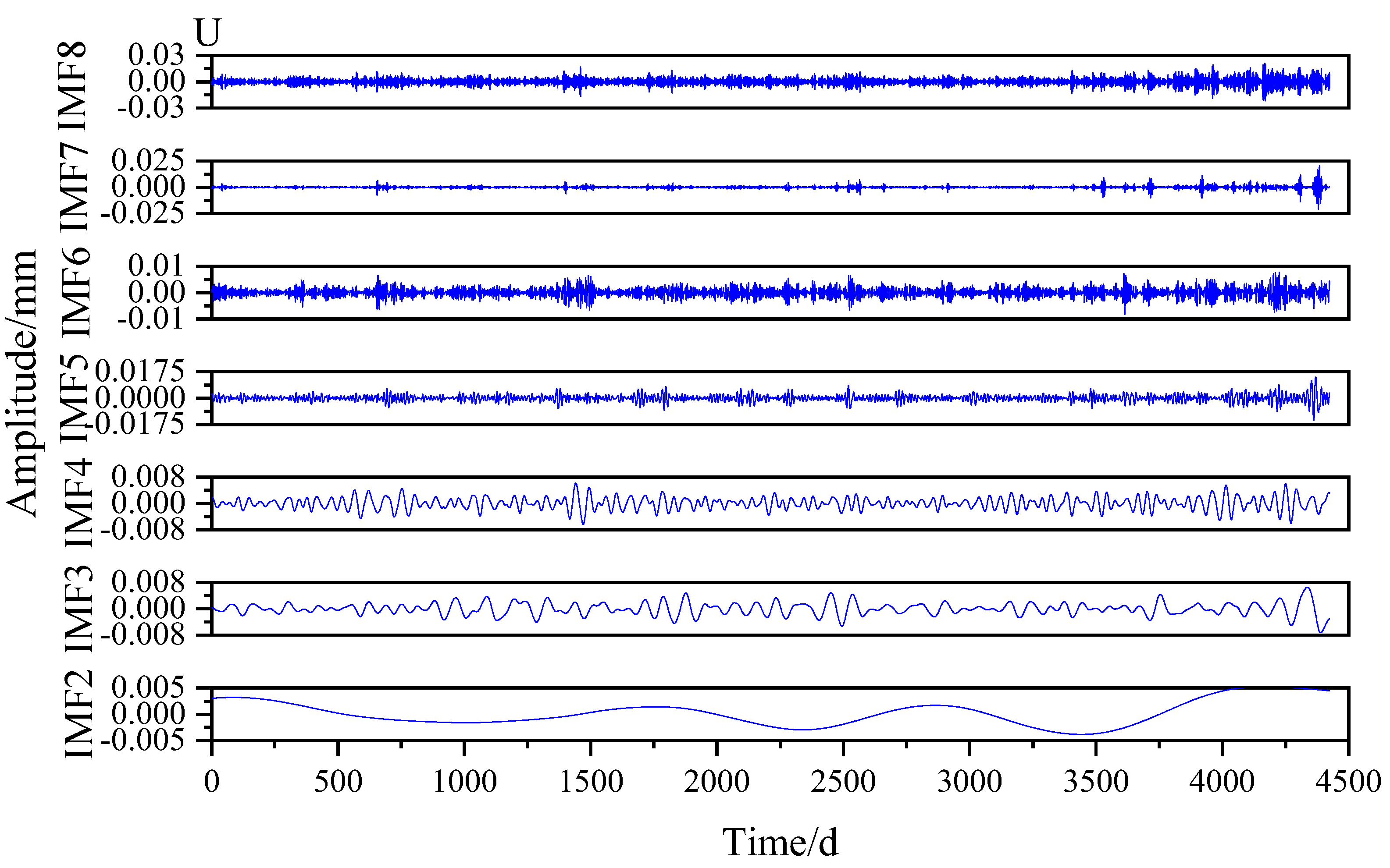
We used the optimal parameter combination obtained from COA to perform VMD decomposition on the signal, and obtained 8 IMF components as shown in Figure 7. From Figure 6, the low-frequency components are mainly concentrated in the first 2 modes.
To effectively separate low-frequency signals and high-frequency noise, it is necessary to calculate the Multi-Scale Permutation Entropy (MPE) values of each IMF component. When calculating MPE, appropriate parameters need to be set. Chen et al. (2023) set the scale factor to 12, embedding dimension to 6, and delay time to 1 [50]; For the setting of key parameters, we also take , , to calculate the permutation entropy mean of each IMF component under different scale factors as the final MPE value. The closer the MPE value is to 1, the greater the random volatility and higher irregularity of the time series. Through experimental analysis, we set the MPE threshold to 0.6 and consider IMF components greater than 0.6 as noise components, while those less than 0.6 are considered low-frequency signal components. The MPE values of each IMF component decomposed by VMD are shown in Figure 8 and Table 1.
From Figure 8 and Table 1, the MPE values of IMF1~IMF8 gradually increase, indicating that the random volatility of the sequence is increasing and the noise components are gradually increasing, which is consistent with the waveform description in Figure 9(a). The MPE values of IMF1~IMF2 are all less than 0.6, therefore, IMF1~IMF2 are reconstructed as low-frequency signals, IMF3~IMF8 are reconstructed as high-frequency noise, and then wavelet decomposition is used to process the high-frequency noise part. The results of COA-VMPE-WD decomposition are shown in Figure 9(b).
3.2. Evaluation of Noise Reduction Effect of Simulated Signals
To further compares the results of WD denoising after MPE judgment reconstruction, we used WD、EMD、EEMD and CEEMDAN to denoise the simulated signals and compared them with COA-VMPE-WD. Figure 10 shows the waveform comparison of the three denoising methods used. From Figure 10, the denoised signal waveforms of WD、EMD、EEMD and CEEMDAN have poor fitting effects with the original sequence, while COA-VMPE-WD, compared to WD、EMD、EEMD and CEEMDAN has a waveform that is closer to the simulated signal after denoising. The curve is smoother, avoiding the endpoint effect and mode mixing problem in the denoising process of EMD and other methods, which can extract more effective signals and achieve better denoising effect. The evaluation indicators for noise reduction using different methods are shown in Table 2.
According to Table 2, for simulated signals, COA-VMPE-WD has the best noise reduction evaluation indicators compared to WD, EMD, EEMD and CEEMDAN methods. The RMSE (0.2291 mm) of COA-VMPE-WD is reduced by 26.5% compared to the suboptimal EMD, and the MAE (0.1780 mm) is reduced by 23.6%, indicating its outstanding residual control ability; The SNR of COA-VMPE-WD (27.8397 dB) is improved by 10.7% compared to EMD, indicating effective separation of noise and signal; The R (0.9757) of COA-VMPE-WD is close to 1, verifying its stronger signal fidelity. EMD is limited by endpoint effects and modal aliasing, and its accuracy is still lower than COA-VMPE-WD. WD、EEMD and CEEMDAN are misaligned due to noise addition strategies, resulting in significant degradation of RMSE and MAE, and a sharp drop in SNR (about 13 dB), reflecting their insufficient anti-interference ability. In summary, the advantage of COA-VMPE-WD lies in the coupled COA optimized VMD, which adaptively decomposes modes through MPE entropy constraints, avoiding the mode mixing problem of traditional EMD series.
3.3. Application of COA-VMPE-WD for GNSS Time Series Denoising Analysis
We conducted experiments on the time series of 52 GNSS stations with E (East), N (North), and U (Up) components using COA-VMPE-VMD, and the processing process was consistent with the simulation signal experiment. Among them, the results of COA optimized VMD parameters in the COA-VMPE-VMD method are shown in Figure 11 and Figure 12, the K value of the U component fluctuates greatly, while the K values of the E and U components are mainly concentrated between 5 and 11, and the values of each component mainly fluctuate within the range of 800 to 3600. We present in the appendix the adaptive curve of FJPT station solved by COA-VMPE-VMD method in Figure A1, the modal number distribution decomposed by COA-VMPE-VMD method in Figure A2, and the IMF value distribution of FJPT station solved by COA-VMPE-VMD method in Figure A3, Figure A4 and Figure A5.
3.4. Comparative Analysis of COA-VMPE-WD
The study takes FJPT station as an example to analyze the performance of COA-VMPE-WD denoising method. Figure 13 shows the denoising effects of five methods: WD, EMD, EEMD, CEEMDAN, and COA-VMPE-WD. From Figure 13, all five methods can effectively extract nonlinear changes from the original data, and the denoised signal exhibits significant periodic changes in the U component. Compared with the other four methods, the COA-VMPE-WD denoised signal has a smoother curve, indicating that it effectively filters out high-frequency noise. However, the denoised signals of the other four methods still contain some high-frequency noise, especially in the EMD method.
Figure 14 shows the residual comparison between the denoised signal obtained using five methods and the original time series. As shown in the figure, the residual fluctuations are significant after EMD and EEMD denoising. The COA-VMPE-WD method obtains the smallest average residual between the denoised signal and the original signal, indicating that this method effectively filters out high-frequency noise and has a more significant denoising effect.
To better demonstrate the effectiveness of our method in denoising GNSS measured data, we evaluated the accuracy of 52 stations after denoising processing. Figure 15 shows the comparison of four evaluation index values of the denoised signals from 52 GNSS reference stations using the above five methods. The results of NEU component are shown in (a) and (b) of Figure 15, Figure 16 and Figure 17. The COA-VMPE-WD method has the smallest RMSE and MAE values, and the WD denoising method has the worst performance The noise reduction effect of EMD method is consistent with that of EEMD method in some stations. Overall, the difference in noise reduction effect between the two methods is not significant and relatively close. The reason for this may be due to the complex crustal tectonic movements in some stations, and further analysis is needed to determine the specific reasons; Compared with CEEMDAN, EMD, and EEMD methods, the RMSE and MAE obtained by denoising with COA-VMPE-WD method are smaller. As shown in Figure 15, Figure 16 and Figure 17, the R (close to 1) and SNR after denoising with COA-VMPE-WD method are larger. All evaluation indicators after denoising with COA-VMPE-WD method are optimal, indicating that its denoising effect is better and it can effectively extract more useful signals.
4. Discussion
4.1. Analysis of Optimal Noise Models Using Different Methods
In order to illustrate the denoising effect of the method proposed in this paper more intuitively, different noise models assume that there are differences in estimating the velocity and uncertainty of the reference station. Therefore, the study selects four types of noise models: FN+WN, FN+RW, FN+RW+WN, and PL+WN (where WN is white noise, FN is flicker noise, RW is random walk noise, and PL is power-law noise). The maximum likelihood estimation method of Hector software is used for analysis. The optimal noise models for the E, N, and U components of each reference station are determined by an improved Bayesian information criterion (BIC_tp) [4], and the noise amplitude and velocity uncertainty of each component before and after denoising in the optimal noise model are obtained. The results are shown in Table 3 to Table 4. As shown in Figure 18.
According to Table3, before denoising, the N component of the original GNSS coordinate time series is dominated by the PLWN noise model, the optimal noise models for the E component coordinate time series are dominated by PLWN and FNRWWN, and the U component is dominated by FNWN and FNRWWN. Table4 shows the optimal noise model of GNSS stations after different denoising methods. Table4 compares the noise type changes of different components (N, E, U) after processing with the original noise model (Origin) and five denoising methods (WD, EMD, EEMD, CEEMDAN, COA-VMPE-WD) On the N-component, the original noise is mainly PLWN, and all denoising methods can effectively preserve the PLWN characteristics without introducing high-order noise, indicating that the methods have good adaptability to the N-component. On the E component, the original noise includes PLWN and FNRWWN. After denoising, most methods (such as WD and EMD) simplify FNRWWN to PLWN. However, COA-VMPE-WD detects the characteristics of FNRW noise at some stations while detecting PLWN. On the U-component, the original noise is mainly FNRWWN and FNWN. After denoising, most methods (such as CEEMDAN) optimize it to PLWN, but COA-VMPE-WD still generates FNRW in FNWN, indicating that COA-VMPE-WD can detect the influence of RW. The U-component noise is more complex, and RW has the greatest impact on the U-component.
4.2. Analysis of GNSS Station Velocity And Annual Term Using Different Methods
Figure 18 shows the noise amplitude distribution of E, N, and U components before and after denoising under the main noise model. According to Table 4, it can be seen that in the E, N, and U components, after denoising by WD, EMD, EEMD, CEEMDAN, and COA-VMPE-WD methods, RW noise can be effectively detected, and the average amplitude of colored noise is also significantly reduced. Moreover, the COA-VMPE-WD method reduces the average amplitude of colored noise compared to the other four methods. Overall, the COA-VMPE-WD method achieves good denoising effect. However, in Figure 18, the U component has the highest amplitude value under the CEEMDAN denoised PLWN model. This may be due to the significant impact of RW in the noise model on the amplitude of denoised PL. When the noise model is PLWN, the amplitude of denoised FN decreases significantly but cannot be completely eliminated. The reason for this phenomenon may be that the noise characteristics of the denoised data have changed, and the noise model does not match FNWN. When using the PLWN model to solve the noise in the denoised signal, RW is transformed into PL.
Figure 19 shows the uncertainty of GNSS station velocity before and after denoising, and the average GNSS station velocity obtained from the denoised signal compared to the original data is shown in Table 5. From Figure 19, it can be seen that the E, N, and U components of the majority of reference stations are denoised using WD, EMD, WD, CEEMDAN, and COA-VMPE-WD methods, resulting in varying degrees of reduction in station velocity and velocity uncertainty for each component. The COA-VMPE-WD method reduces the average velocity of GNSS stations after denoising by 44.44%, 50.00%, 52.38%and 44.44% compared to the WD, EMD, EEMD, and CEEMDAN methods with N-component, respectively. On the E component, the COA-VMPE-WD method reduced station velocity by an average of 14.29%, 18.18%, 21.74%, and 21.74% compared to the WD, EMD, EEMD, and CEEMDAN methods. On the U component, the COA-VMPE-WD method reduced station velocity by an average of 50.00%, 59.09%, 18.18%, and 64.00% compared to the WD, EMD, EEMD, and CEEMDAN methods. To sum up, the CEEMDAN method has the most significant effect on reducing velocity uncertainty, followed by the WD method. The EMD and EEMD methods are poor and both have situations where the velocity uncertainty of some reference stations increases (such as the U component of SDCY station, the E component of XJBL station, etc.).
According to Table 5, on the N component, the original mean station velocity is 0.018mm/a, while WD and CEEMDAN maintain their original values. EMD and EEMD slightly increase (0.020mm/a-0.021 mm/a), while COA-VMPE-WD significantly decreases to 0.010 mm/a, indicating that this method has the strongest noise suppression effect on the N component. On the E component, the original mean station velocity is 0.023 mm/a, and the results of various methods are relatively close (0.018 mm/a -0.023 mm/a). Among them, COA-VMPE-WD has the largest reduction (0.018 mm/a), while other methods basically maintain the original characteristics. On the U component, there are significant differences between different methods: EMD remains at its original value, CEEMDAN increases to 0.025 mm/a, EEMD and COA-VMPE-WD decrease to 0.011 mm/a and 0.009 mm/a, respectively, reflecting the complex noise characteristics of the U component and the significant differences in processing effects between different algorithms. In summary, COA-VMPE-WD exhibits strong noise suppression ability for all components, while CEEMDAN may excessively preserve noise features for the U component. There are significant differences in the response characteristics of denoising methods for different components, and the U component has the highest dispersion in processing effect.
5. Conclusions
The study proposes a COA-VMPE-WD denoising algorithm based on the nonlinear and non-stationary characteristics of GNSS coordinate time series. In response to the problem that traditional VMD cannot adaptively determine the values of modal number and penalty factor [,]in the denoising process, resulting in insufficient signal decomposition or over decomposition affecting the effective denoising of time series, a COA optimized VMD parameter with envelope entropy as the fitness function is proposed. Multi scale permutation entropy (MPE) is used as the screening criterion for noise and signal, and wavelet decomposition algorithm (WD) is combined to improve VMD. This article conducts noise reduction research and analysis through simulated signals and measured data from 52 GNSS stations, verifying the reliability and effectiveness of the method. It compares it with traditional WD, EMD, EEMD, and CEEMDAN method. Our main conclusions are as follows:
- (1)
- Simulation signal experiments show that compared to traditional EMD and WD methods, VMD method can effectively alleviate modal aliasing and endpoint effects, and has better signal feature extraction ability. In terms of noise reduction, the COA-VMPE-WD method outperforms the WD, EMD, EEMD, and CEEMDAN methods in terms of RMSE, R, and SNR evaluation metrics, effectively removing noise from the original data.
- (2)
- Experimental data shows that WD, EMD, EEMD, and CEEMDAN methods can remove white noise from the original coordinate time series and significantly reduce the amplitude of colored noise. Compared with WD, EMD, EEMD, and CEEMDAN methods, COA-VMPE-WD has a more significant noise reduction effect and better preserves the characteristics of the original signal.
- (3)
- The WD, EMD, EEMD, CEEMDAN COA-VMPE-WD methods have a significant impact on the U-component in terms of the velocity and uncertainty of the reference station, the COA-VMPE-WD method reduced station velocity by an average of 50.00%, 59.09%, 18.18%, and 64.00% compared to the WD, EMD, EEMD, and CEEMDAN methods, The noise reduction effect is higher than the other four methods. The above results verify the effectiveness and reliability of the COA-VMPE-WD denoising method. However, the method proposed in this paper reduces computational efficiency to a certain extent. Therefore, further research is needed on how to construct a simple and efficient denoising method based on VMD.
Author Contributions
Y.Z., writing—original draft preparation and data processing and figure plotting.; X.H., methodology, review, and editing the manuscript.; All authors have read and agreed to the published version of the manuscript.
Funding
This work is sponsored by National Natural Science Foundation of China (42364002), Major Discipline Academic and Technical Leaders Training Program of Jiangxi Province (20225BCJ23014).
Data Availability Statement
The processing of Station data can be obtained at http://www.cgps.ac.cn/.
Conflicts of Interest
Author Ziyu Wang was employed by the company Xuzhou Surveying & Mapping Research Institute Co., Ltd. The remaining authors declare that the research was conducted in the absence of any commercial or financial relationships that could be construed as a potential conflict of interest.
Appendix A
Figure A1.
FJPT station three component adaptive value.
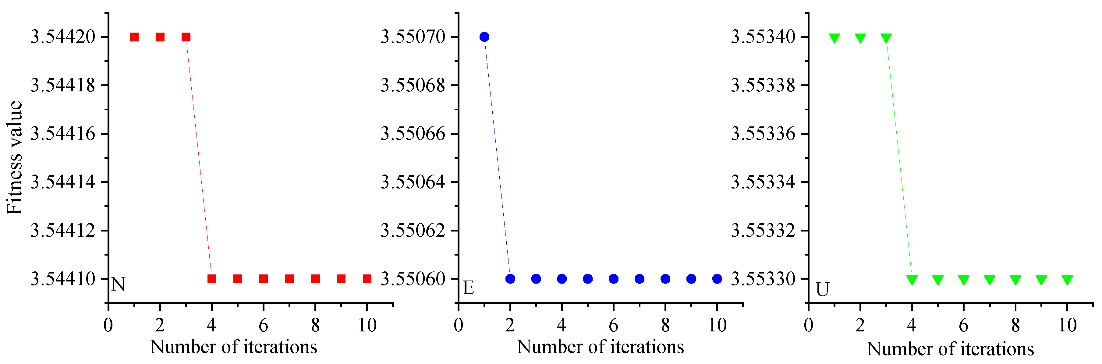
Figure A2.
Distribution of three component MPE values at FJPT station.
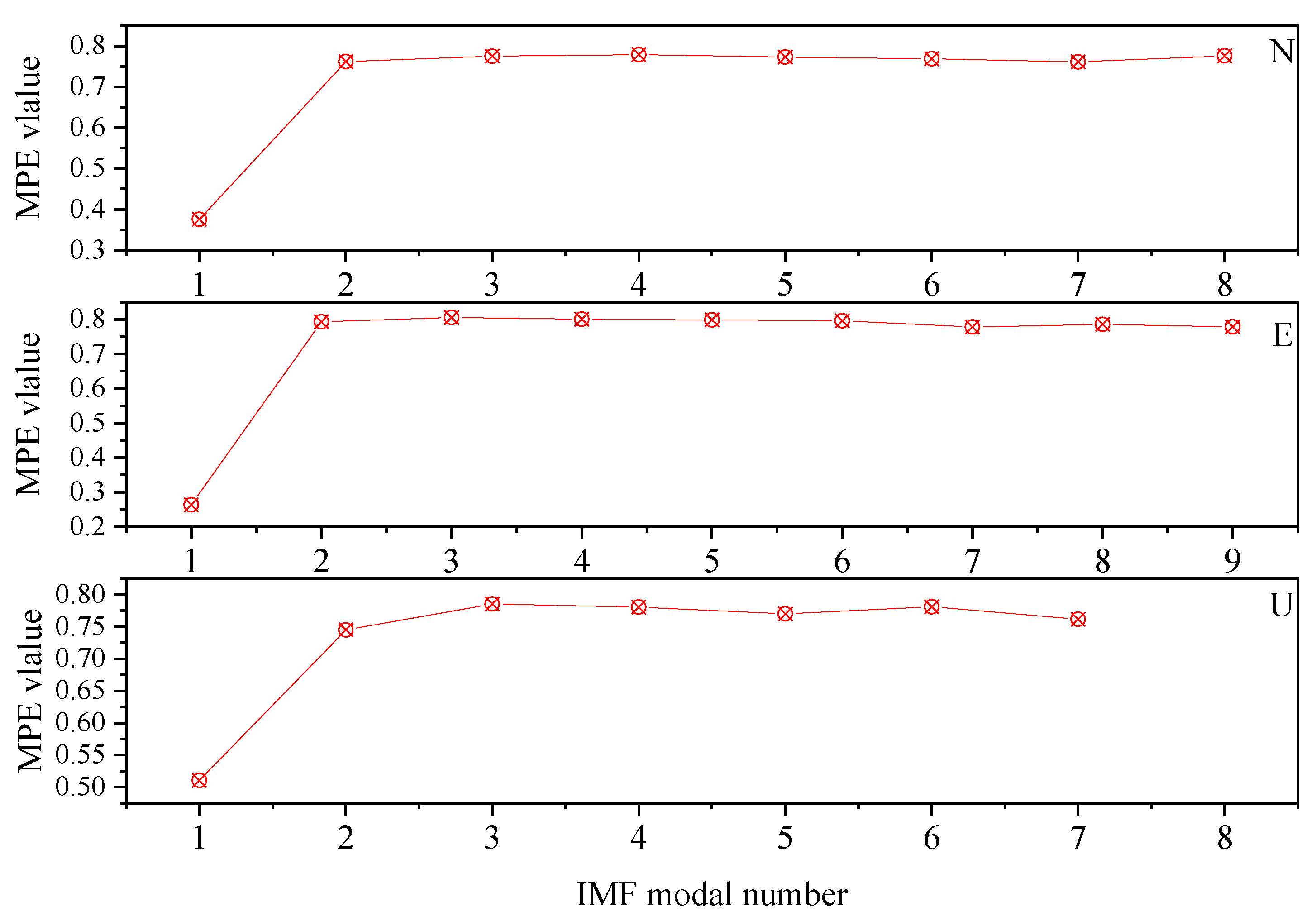
Figure A3.
N-component IMF distribution of FJPT station.
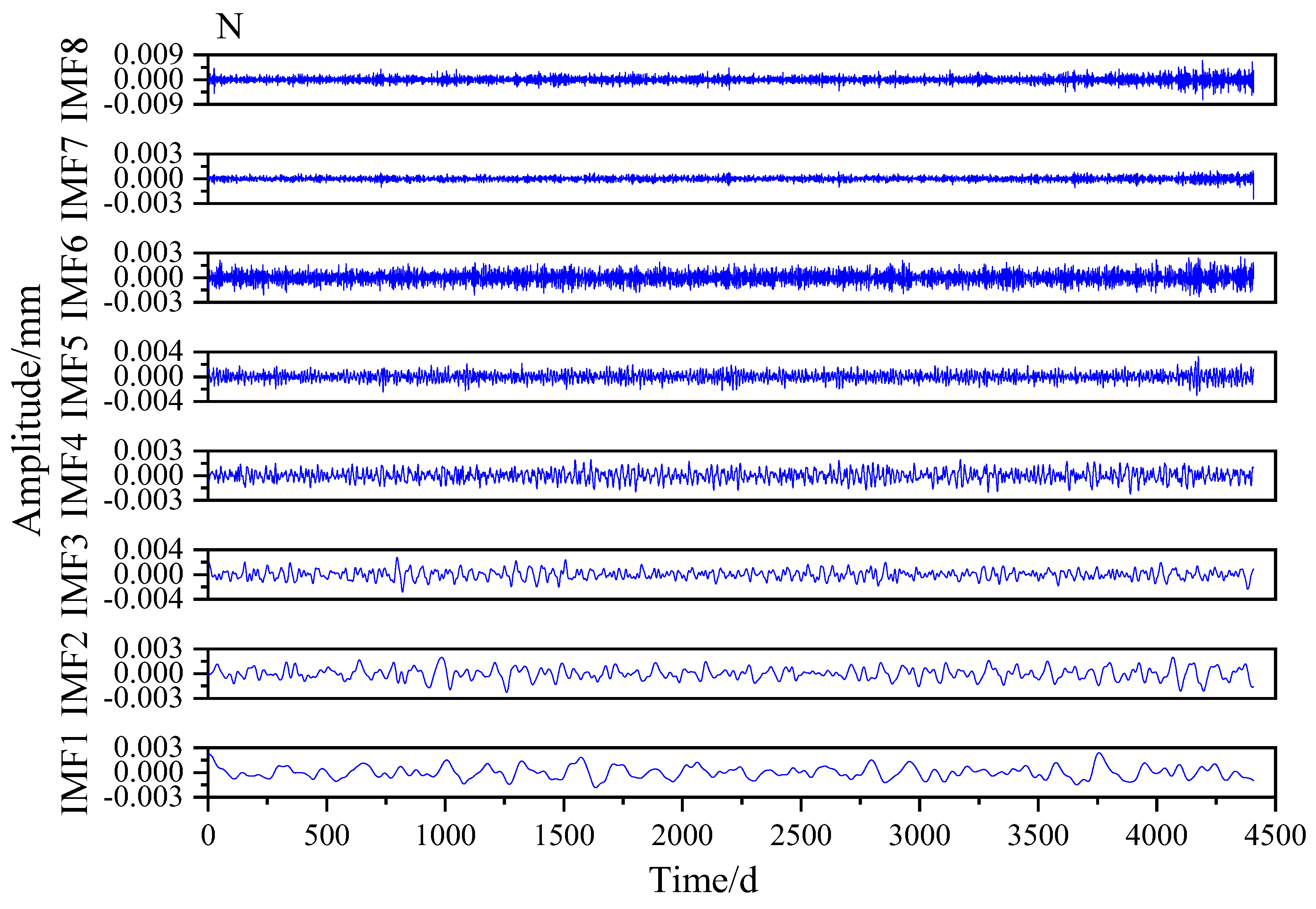
Figure A4.
E-component IMF distribution of FJPT station.
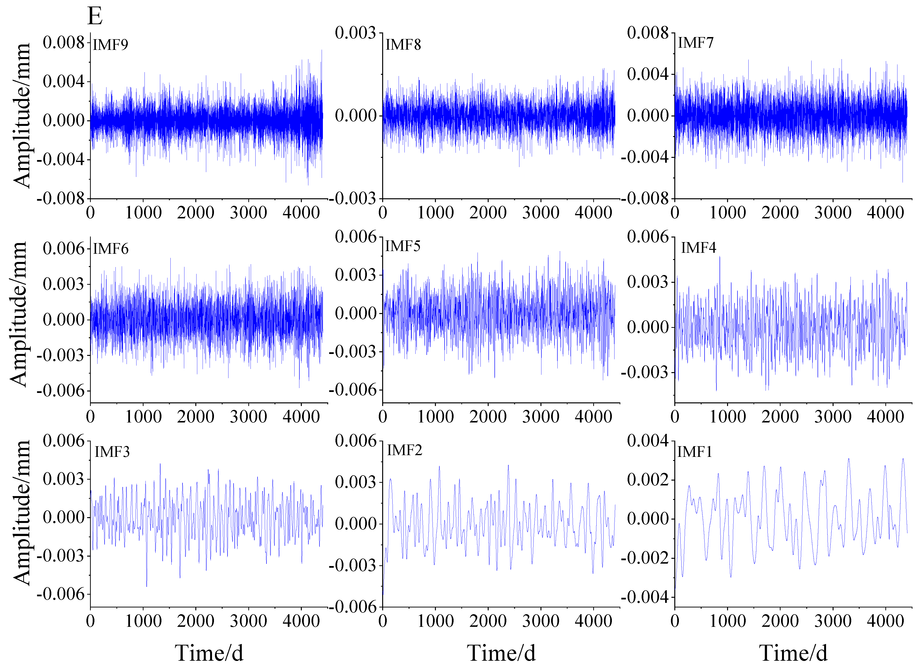
Figure A5.
U-component IMF distribution of FJPT station.
References
- Klos, A. , Bogusz, J., Bos, M. S., & Gruszczynska, M. Modelling the GNSS time series: different approaches to extract seasonal signals. Geodetic time series analysis in earth sciences. Cham: Springer International Publishing. 2019, 211-237.
- Kaczmarek, A. , & Kontny, B. Identification of the noise model in the time series of GNSS stations coordinates using wavelet analysis. Remote Sensing 2018, 10, 1611. [Google Scholar]
- Montillet, J. P. , Tregoning, P., McClusky, S., & Yu, K. Extracting white noise statistics in GPS coordinate time series. IEEE Geoscience and Remote Sensing Letters 2012, 10, 563–567. [Google Scholar] [CrossRef]
- He, X. , Bos, M. S., Montillet, J. P., & Fernandes, R. M. S. Investigation of the noise properties at low frequencies in long GNSS time series. Journal of Geodesy 2019, 93, 1271–1282. [Google Scholar] [CrossRef]
- Dmitrieva, K. , Segall, P., & Bradley, A. M. Effects of linear trends on estimation of noise in GNSS position time series. Geophysical Journal International 2016, ggw391. [Google Scholar] [CrossRef]
- Langbein, J. Methods for rapidly estimating velocity precision from GNSS time series in the presence of temporal correlation: a new method and comparison of existing methods. Journal of Geophysical Research: Solid Earth 2020, 125, e2019JB019132. [Google Scholar] [CrossRef]
- Benoist, C. , Collilieux, X., Rebischung, P., Altamimi, Z., Jamet, O., Métivier, L.,... & Bel, L. Accounting for spatiotemporal correlations of GNSS coordinate time series to estimate station velocities. Journal of Geodynamics 2020, 135, 101693. [Google Scholar] [CrossRef]
- Arias-Gallegos, A. , Borque-Arancón, M. J., & Gil-Cruz, A. J. Present-Day Crustal Velocity Field in Ecuador from GPS Position Time Series. Sensors 2023, 23, 3301. [Google Scholar] [CrossRef]
- Rebischung, P. , & Gobron, K. Modeling random isotropic vector fields on the sphere: theory and application to the noise in GNSS station position time series. Journal of Geodesy 2024, 98, 79. [Google Scholar] [CrossRef]
- Jagoda, M. , & Rutkowska, M. An analysis of the Eurasian tectonic plate motion parameters based on GNSS stations positions in ITRF2014. Sensors 2020, 20, 6065. [Google Scholar] [PubMed]
- Jagoda, M. Determination of motion parameters of selected major tectonic plates based on GNSS station positions and velocities in the ITRF2014. Sensors 2021, 21, 5342. [Google Scholar] [CrossRef]
- He, X. , Yu, K., Montillet, J. P., Xiong, C., Lu, T., Zhou, S.,... & Ming, F. GNSS-TS-NRS: An Open-source MATLAB-Based GNSS time series noise reduction software. Remote Sensing 2020, 12, 3532. [Google Scholar] [CrossRef]
- Wang, X. , Hou, Z., Xu, K., Hu, X., Gao, X., & Zhang, Z. Noise Reduction of GNSS Coordinate Time Series Based on Adaptive Wavelet Basis Optimization and an Improved Threshold Function. Measurement Science and Technology 2025. [Google Scholar] [CrossRef]
- Li, X. , Zhang, S., Dong, Z., Dou, X., Xue, Y., Wang, L.,... & Li, P. Research on GNSS time series noise reduction combining principal component decomposition and compound evaluation index. China Satellite Navigation Conference (CSNC 2021) Proceedings: Volume III. Singapore: Springer Singapore, 2021; 378–386. [Google Scholar]
- Ma, J. , Cao, C. D., Jiang, W. P., & Zhou, L. Elimination of colored noise in GNSS station coordinate time series by using wavelet packet coefficient information entropy. Geomatics and Information Science of Wuhan University 2021, 46, 1309–1317. [Google Scholar]
- Ji, K. , Shen, Y., & Wang, F. Signal extraction from GNSS position time series using weighted wavelet analysis. Remote Sensing 2020, 12, 992. [Google Scholar] [CrossRef]
- Chen, Q. , van Dam, T., Sneeuw, N., Collilieux, X., Weigelt, M., & Rebischung, P. Singular spectrum analysis for modeling seasonal signals from GPS time series. Journal of Geodynamics 2013, 72, 25–35. [Google Scholar] [CrossRef]
- Khazraei, S. M. , & Amiri-Simkooei, A. R. On the application of Monte Carlo singular spectrum analysis to GPS position time series. Journal of Geodesy 2019, 93, 1401–1418. [Google Scholar] [CrossRef]
- Zhang, S. , Li, Z., He, Y., Hou, X., He, Z., & Wang, Q. Extracting of periodic component of GNSS vertical time series using EMD. Sci. Surv. Mapp 2018, 43, 80–84. [Google Scholar]
- Yu, L. , Gao, Y., Jijian, L., Li, F., Gao, X., & Wang, T. Improving GNSS-RTK multipath error extraction with an integrated CEEMDAN and STD-based PCA algorithm. GPS Solutions 2024, 28, 192. [Google Scholar] [CrossRef]
- Kunpu, J. , & Yunzhong, S.. Dyadic wavelet transform and signal extraction of GNSS coordinate time series with missing data. Acta Geodaetica et Cartographica Sinica 2020, 49, 537. [Google Scholar]
- Dong, D. , Fang, P., Bock, Y., Cheng, M. K., & Miyazaki, S. I. Anatomy of apparent seasonal variations from GPS-derived site position time series. Journal of Geophysical Research: Solid Earth 2002, 107, ETG–9. [Google Scholar] [CrossRef]
- Liu, X. , Ding, Z., Li, Y., & Liu, Z. Application of EMD to GNSS time series periodic term processing. Geomatics and Information Science of Wuhan University 2023, 48, 135–145. [Google Scholar]
- Yeh, J. R. , Shieh, J. S., & Huang, N. E. Complementary ensemble empirical mode decomposition: A novel noise enhanced data analysis method. Advances in adaptive data analysis 2010, 2, 135–156. [Google Scholar] [CrossRef]
- Agnieszka, W. , & Dawid, K. Modeling seasonal oscillations in GNSS time series with Complementary Ensemble Empirical Mode Decomposition. GPS Solutions 2022, 26, 101. [Google Scholar] [CrossRef]
- Dragomiretskiy, K. , & Zosso, D. Variational mode decomposition. IEEE transactions on signal processing 2013, 62, 531–544. [Google Scholar] [CrossRef]
- Li, W. , & Guo, J. Extraction of periodic signals in Global Navigation Satellite System (GNSS) vertical coordinate time series using the adaptive ensemble empirical modal decomposition method. Nonlinear Processes in Geophysics 2024, 31, 99–113. [Google Scholar] [CrossRef]
- Yuan, Y. , Yan, P., Zhou, H., Huang, Q., Wu, D., Zhu, J., & Ni, Z. Noise reduction and feature enhancement of hob vibration signal based on parameter adaptive VMD and autocorrelation analysis. Measurement Science and Technology 2022, 33, 125116. [Google Scholar] [CrossRef]
- Qi, G. , Zhao, Z., Zhang, R., Wang, J., Li, M., Shi, X., & Wang, H. Optimized VMD algorithm for signal noise reduction based on TDLAS. Journal of Quantitative Spectroscopy and Radiative Transfer 2024, 312, 108807. [Google Scholar] [CrossRef]
- Liu, W. , Cao, S., & Wang, Z. Application of variational mode decomposition to seismic random noise reduction. Journal of Geophysics and Engineering 2017, 14, 888. [Google Scholar] [CrossRef]
- Sun, X. , Lu, T., Hu, S., Wang, H., Wang, Z., He, X.,... & Zhang, Y. A New Algorithm for Predicting Dam Deformation Using Grey Wolf-Optimized Variational Mode Long Short-Term Neural Network. Remote Sensing 2024, 16, 3978. [Google Scholar] [CrossRef]
- Lu, T. , & Xie, J.Deformation monitoring data de-noising method based on variational mode de-composition combined with sample entropy. J. Geod. Geodyn. 2021, 41, 1–6. [Google Scholar]
- Jia, H. , Zhou, X., Zhang, J., Abualigah, L., Yildiz, A. R., & Hussien, A. G Modified crayfish optimization algorithm for solving multiple engineering application problems. Artificial Intelligence Review 2024, 57, 127. [Google Scholar] [CrossRef]
- Jia, H. , Rao, H., Wen, C., & Mirjalili, S. Crayfish optimization algorithm. Artificial Intelligence Review 2023, 56, 1919–1979. [Google Scholar] [CrossRef]
- Ezugwu, A. E. , Shukla, A. K., Nath, R., Akinyelu, A. A., Agushaka, J. O., Chiroma, H., & Muhuri, P. K. Metaheuristics: a comprehensive overview and classification along with bibliometric analysis. Artificial Intelligence Review 2021, 54, 4237–4316. [Google Scholar] [CrossRef]
- Zhang, Y. , Liu, P., & Li, Y. Implementation of an enhanced crayfish optimization algorithm. Biomimetics 2024, 9, 341. [Google Scholar] [CrossRef]
- Chen, X. , Yang, Z., Tian, Z., Yang, B., & Liang, P. Denoising Method for GNSS Time Series Based on GA-VMD and Multi-scale Permutation Entropy. Geomatics and Information Science of Wuhan University 2023, 48, 1425–1434. [Google Scholar]
- Zanin, M. , Zunino, L., Rosso, O. A., & Papo, D. Permutation entropy and its main biomedical and econophysics applications: A review. Entropy 2012, 14, 1553–1577. [Google Scholar] [CrossRef]
- Lu, T. , He, J., He, X., & Tao, R. GNSS coordinate time series denoising method based on parameter-optimized variational mode decomposition. Geomatics and Information Science of Wuhan University 2024, 49, 1856–1866. [Google Scholar]
- Starck, J. L. , Fadili, J., & Murtagh, F. The undecimated wavelet decomposition and its reconstruction. IEEE transactions on image processing 2007, 16, 297–309. [Google Scholar] [CrossRef]
- Soltani, S. . On the use of the wavelet decomposition for time series prediction. Neurocomputing 2002, 48, 267–277. [Google Scholar] [CrossRef]
- Ji, K. , Shen, Y., & Wang, F. Signal extraction from GNSS position time series using weighted wavelet analysis. Remote Sensing 2020, 12, 992. [Google Scholar]
- Hao, F. E. N. G. , Xiao-dan, S. H. I., Xiao-min, H. U. A. N. G., & Zhi-jie, Z. H. A. N. G. Signal de-noising method based on wavelet decomposition. Journal of Measurement Science & Instrumentation 2014, 5. [Google Scholar]
- Quellec, G. , Lamard, M., Josselin, P. M., Cazuguel, G., Cochener, B., & Roux, C. Optimal wavelet transforms for the detection of microaneurysms in retina photographs. IEEE transactions on medical imaging 2008, 27, 1230–1241. [Google Scholar] [PubMed]
- Briggs, R. J. Transformation of Small-Signal Energy and Momentum of Waves. Journal of Applied Physics 1964, 35, 3268–3272. [Google Scholar] [CrossRef]
- Huang, J. , He, X., Hu, S., & Ming, F. Impact of offsets on GNSS time series stochastic noise properties and velocity estimation. Advances in Space Research 2025, 75, 3397–3413. [Google Scholar] [CrossRef]
- Zhou, Y. , He, X., Montillet, J. P., Wang, S., Hu, S., Sun, X.,... & Ma, X. An improved ICEEMDAN-MPA-GRU model for GNSS height time series prediction with weighted quality evaluation index. GPS Solutions 2025, 29, 113. [Google Scholar] [CrossRef]
- Sun, X. , Lu, T., & Wang, Z. Comparative Analysis of Different Deep Learning Algorithms for the Prediction of Marine Environmental Parameters Based on CMEMS Products. Acta Geodyn. Geomater. 2024, 21, 343–363. [Google Scholar]
- Sun, X. , Lu, T., Hu, S., Huang, J., He, X., Montillet, J. P.,... & Huang, Z The relationship of time span and missing data on the noise model estimation of GNSS time series. Remote Sensing 2023, 15, 3572. [Google Scholar] [CrossRef]
- Chen, X. , Yang, Z., Tian, Z., Yang, B., & Liang, p. Denoising Method for GNSS Time Series Based on GA-VMD and Multi-scale Permutation Entropy. Geomatics and Information Science of Wuhan University 2023, 48, 1425–1434. [Google Scholar] [CrossRef]
Figure 1.
GNSS station distributed.
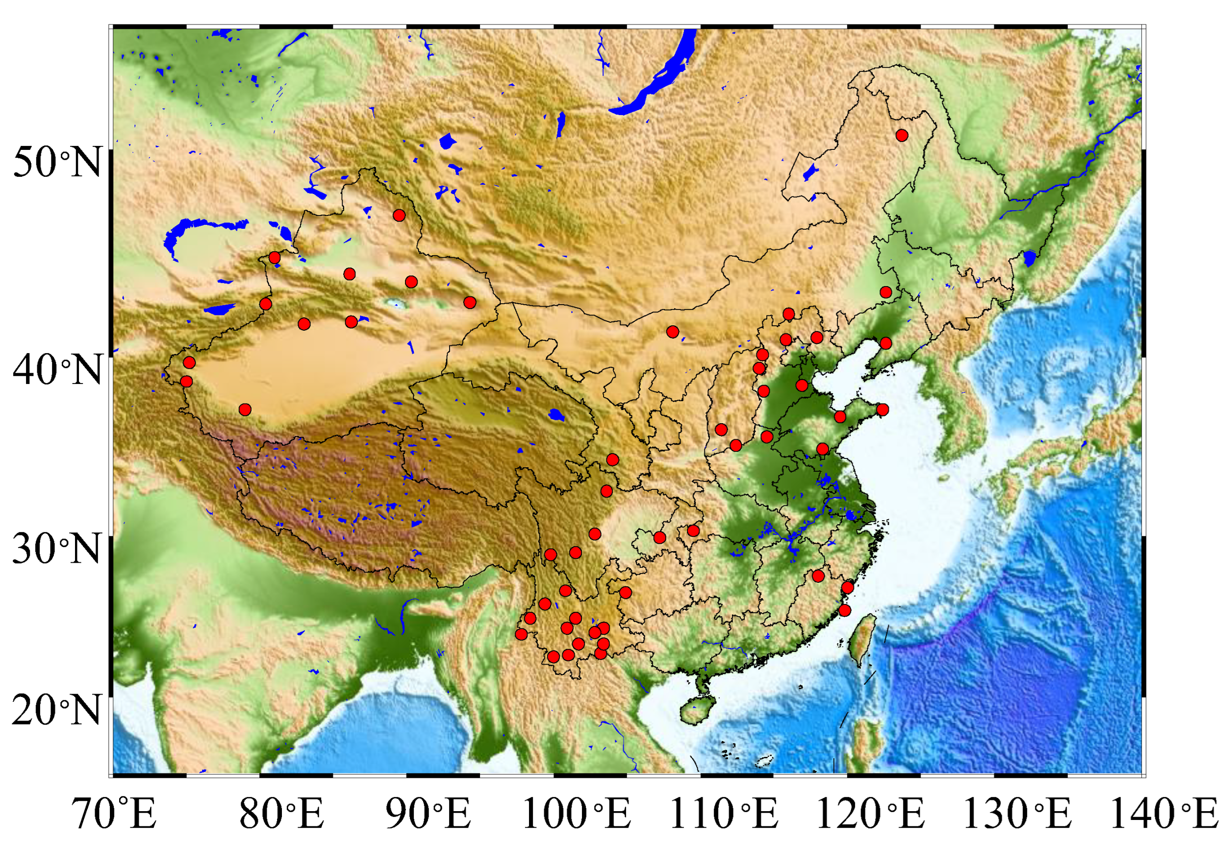
Figure 2.
Basic framework diagram of COA algorithm.
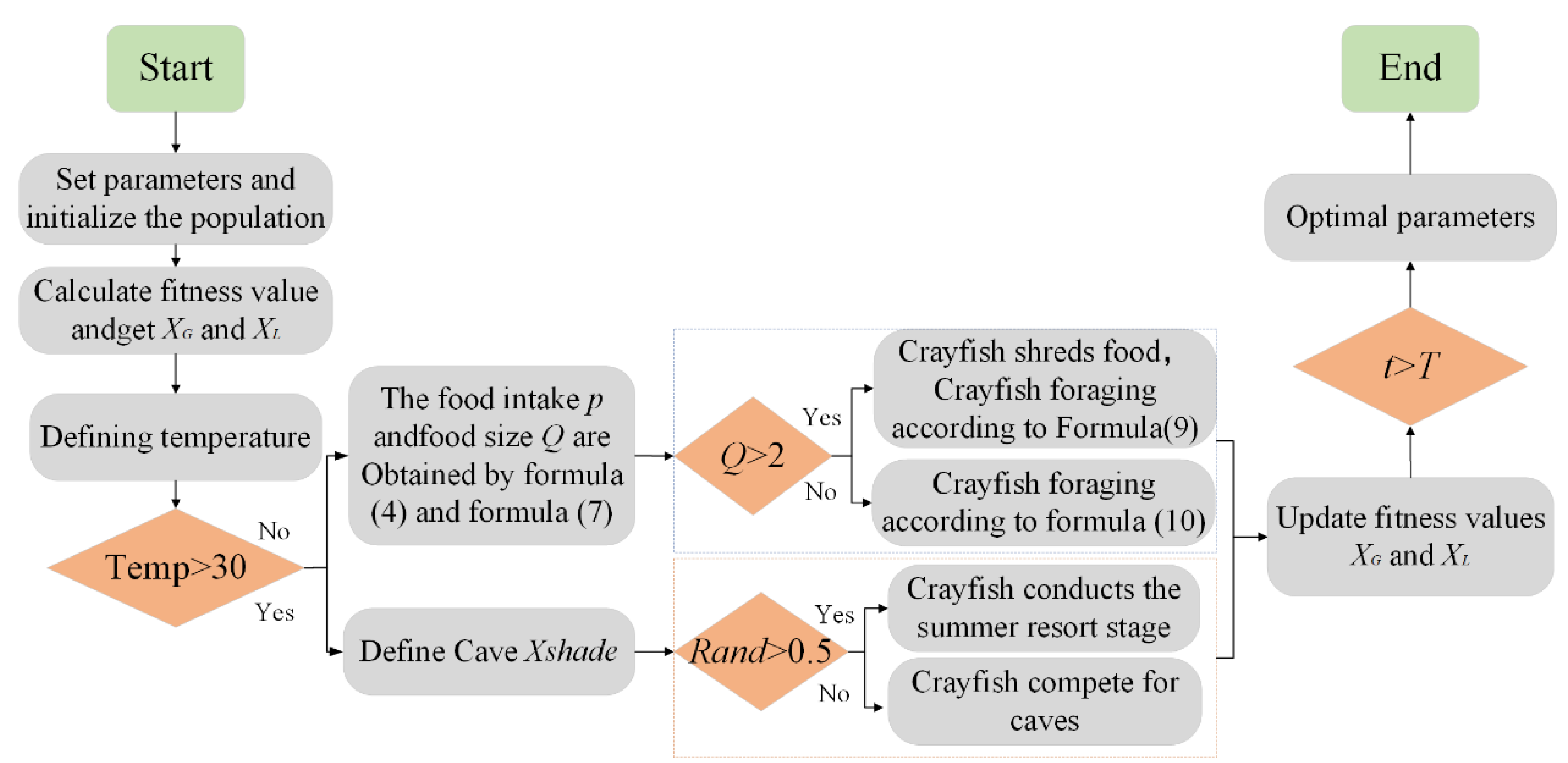
Figure 3.
COA optimized VMD flowchart.
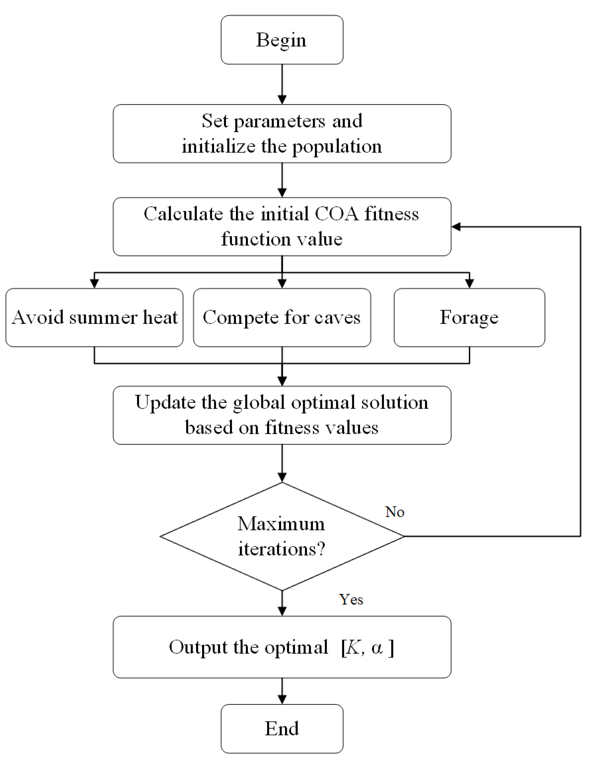
Figure 4.
COA-VMPE flowchart.
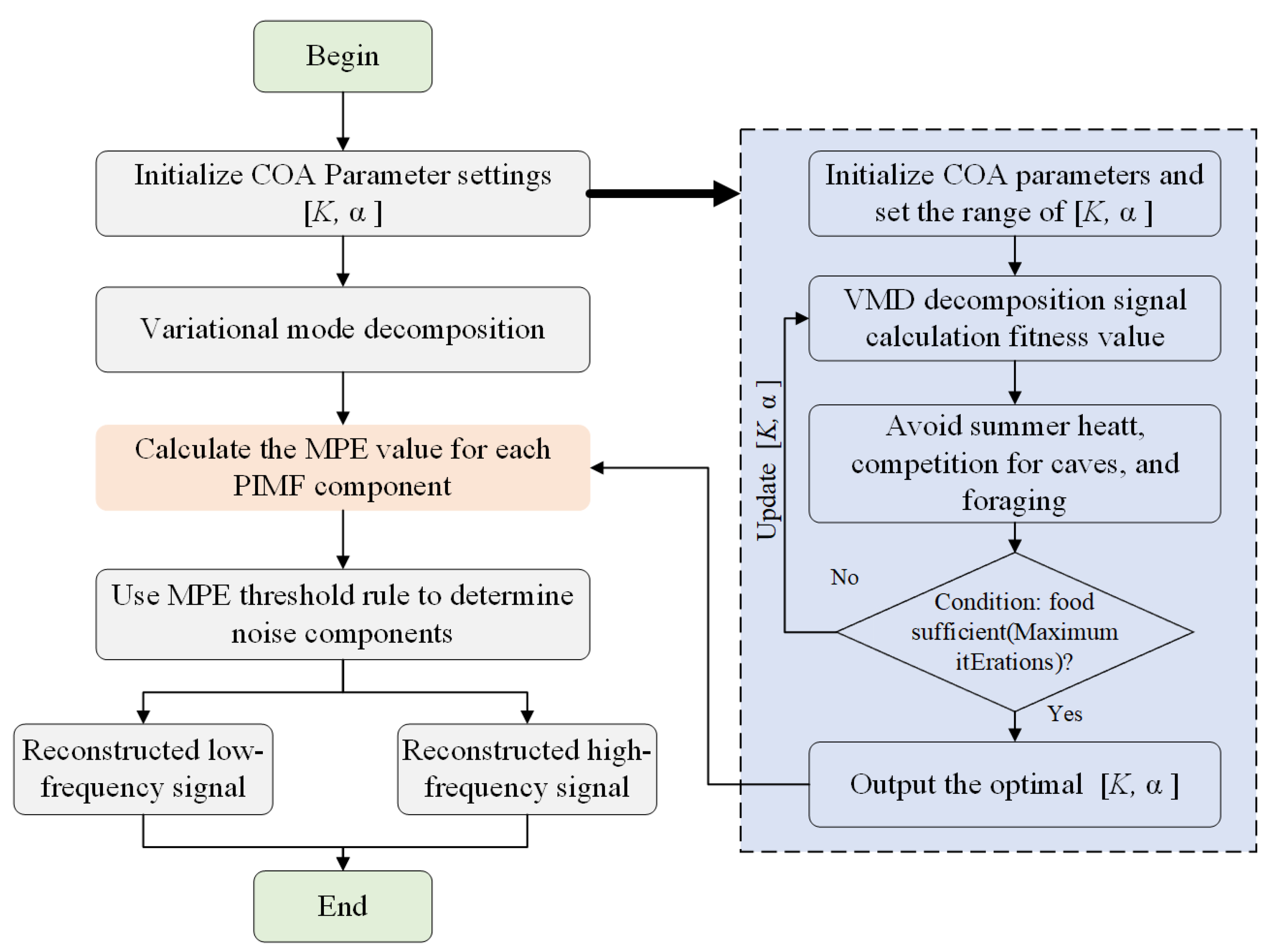
Figure 5.
Frame diagram of COA-VMPE-WD algorithm in the study.
Figure 6.
Convergence Diagram of fitness Values.
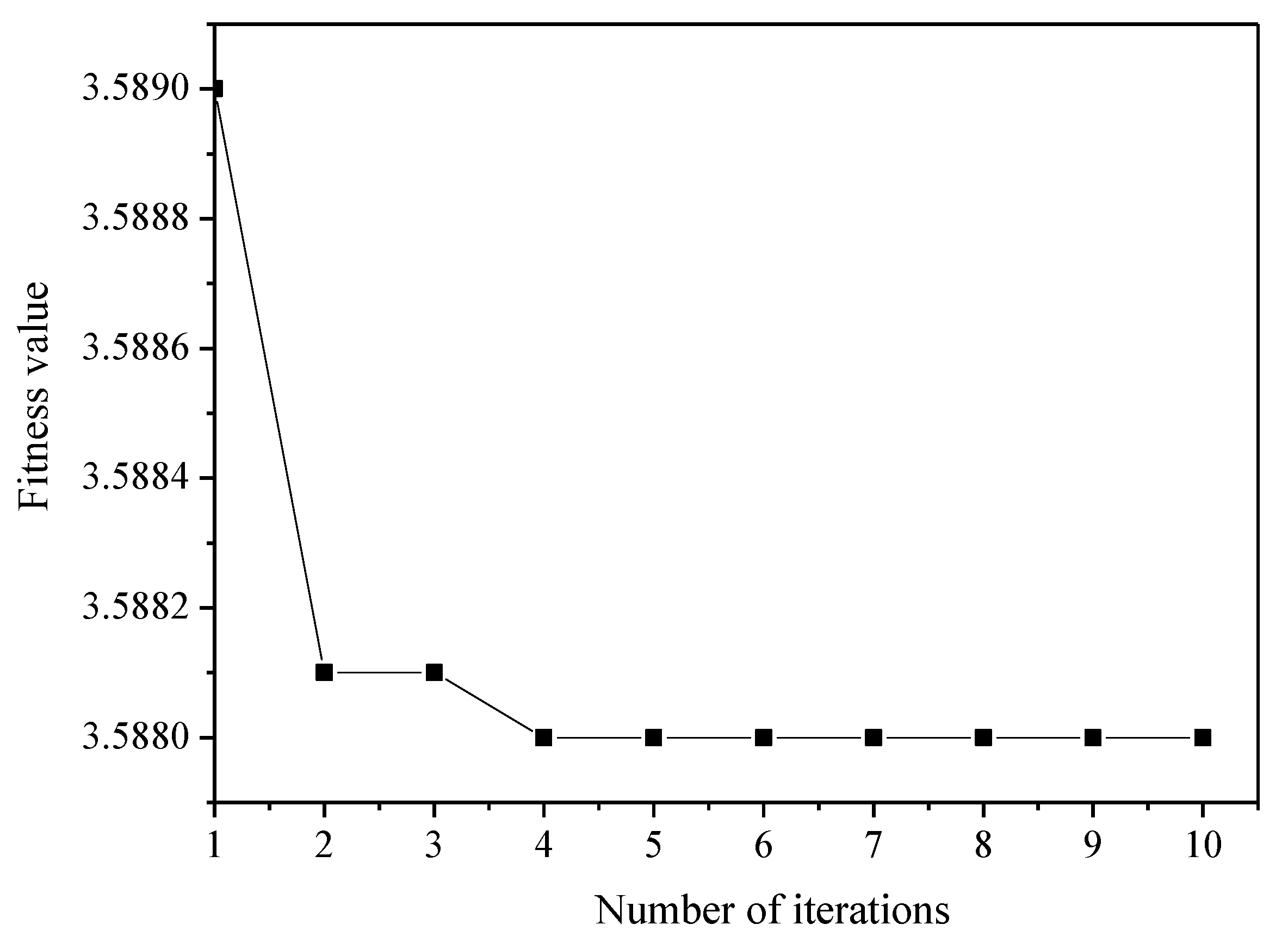
Figure 7.
The distribution of various modes after COA-VVD decomposition.
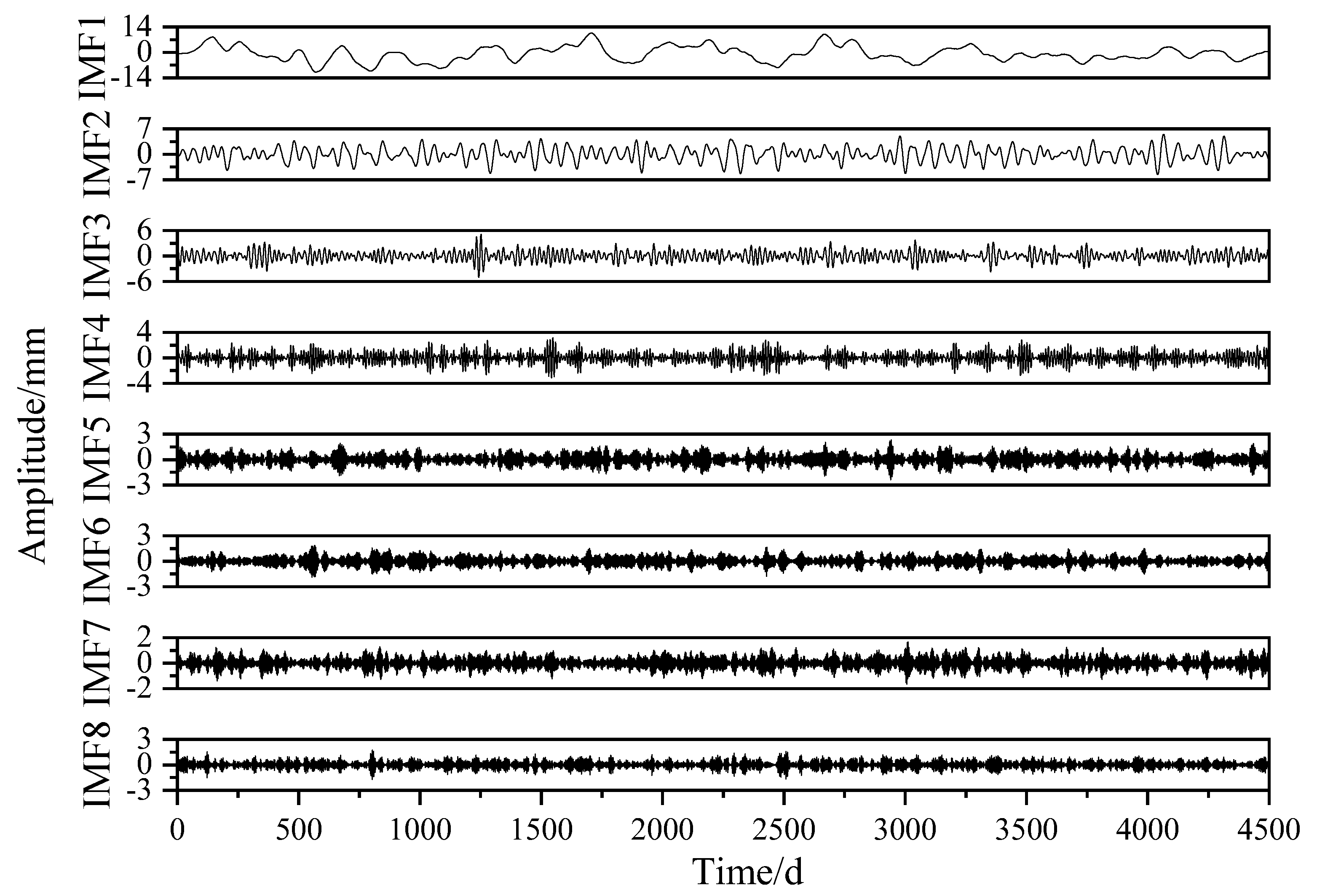
Figure 8.
MPE values of each IMF component.
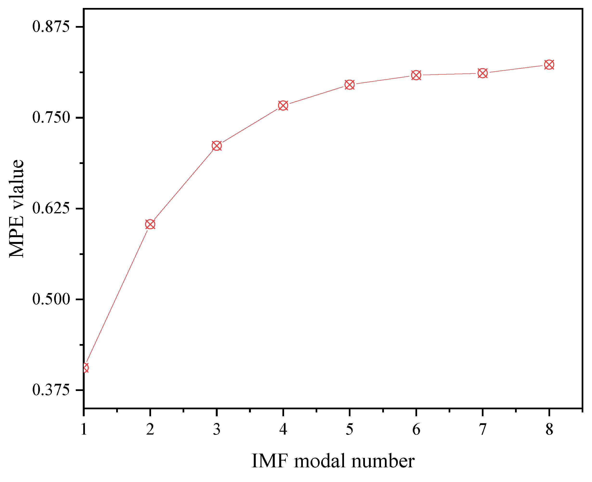
Figure 9.
COA-VMPE-WD decomposition results.
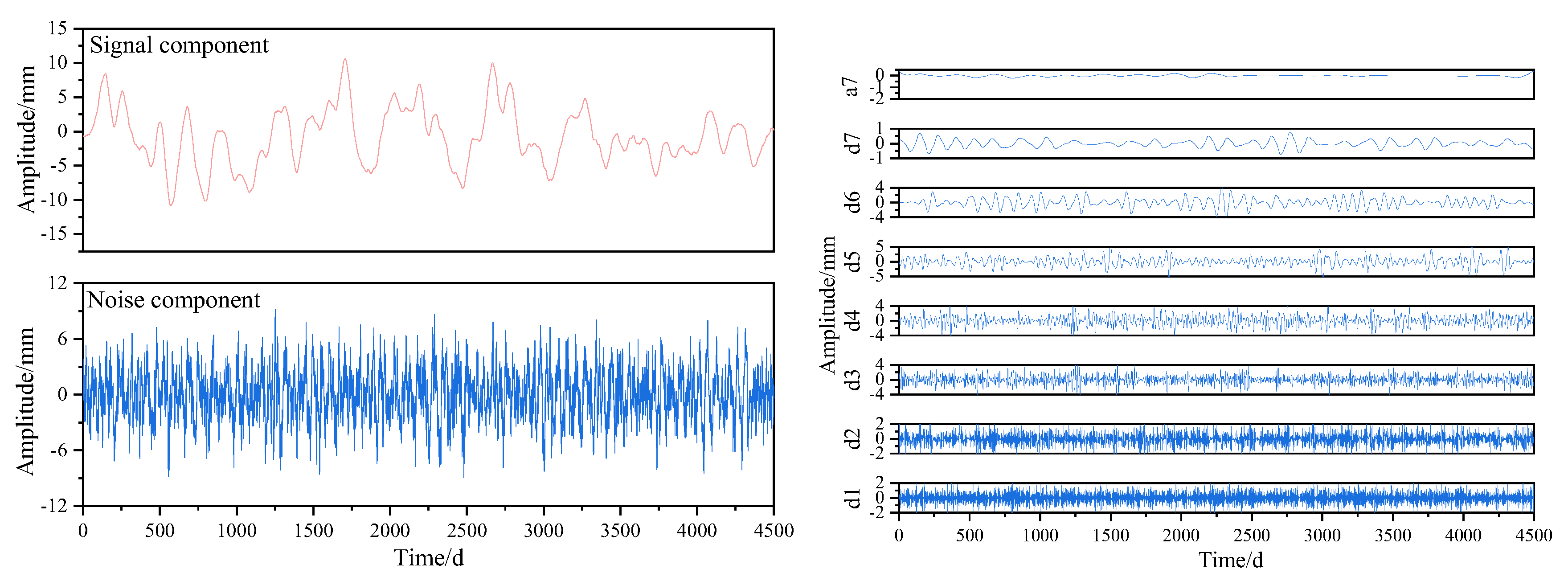
Figure 10.
Simulation signal and three types of noise reduction signals.
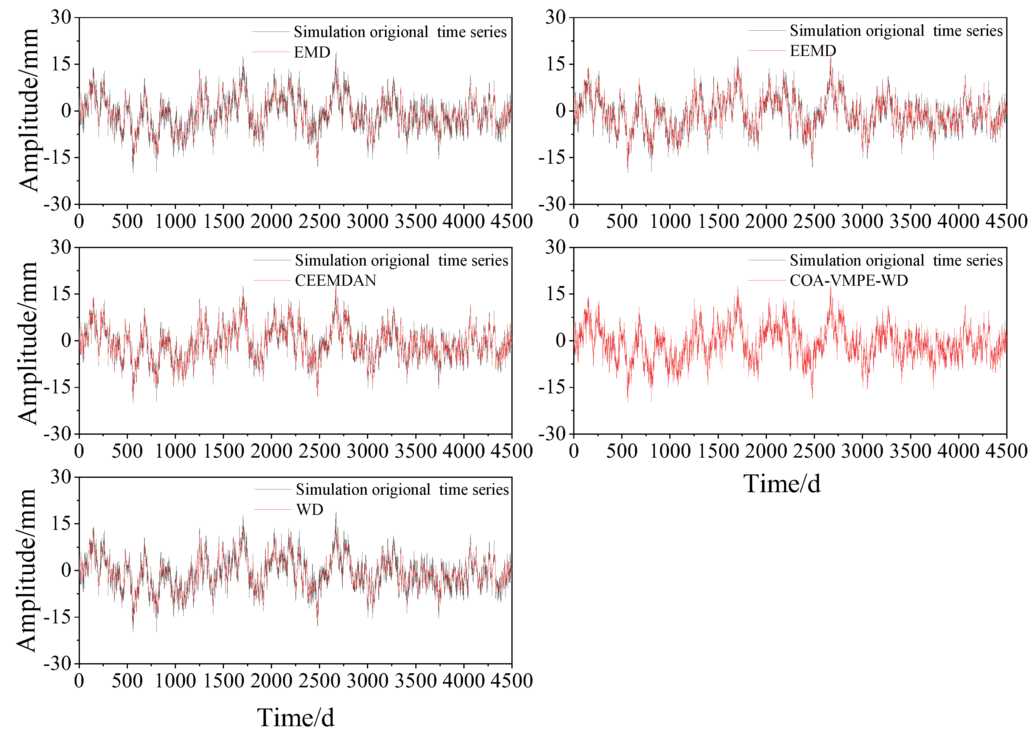
Figure 11.
Distribution of optimal parameter K values for GNSS stations.
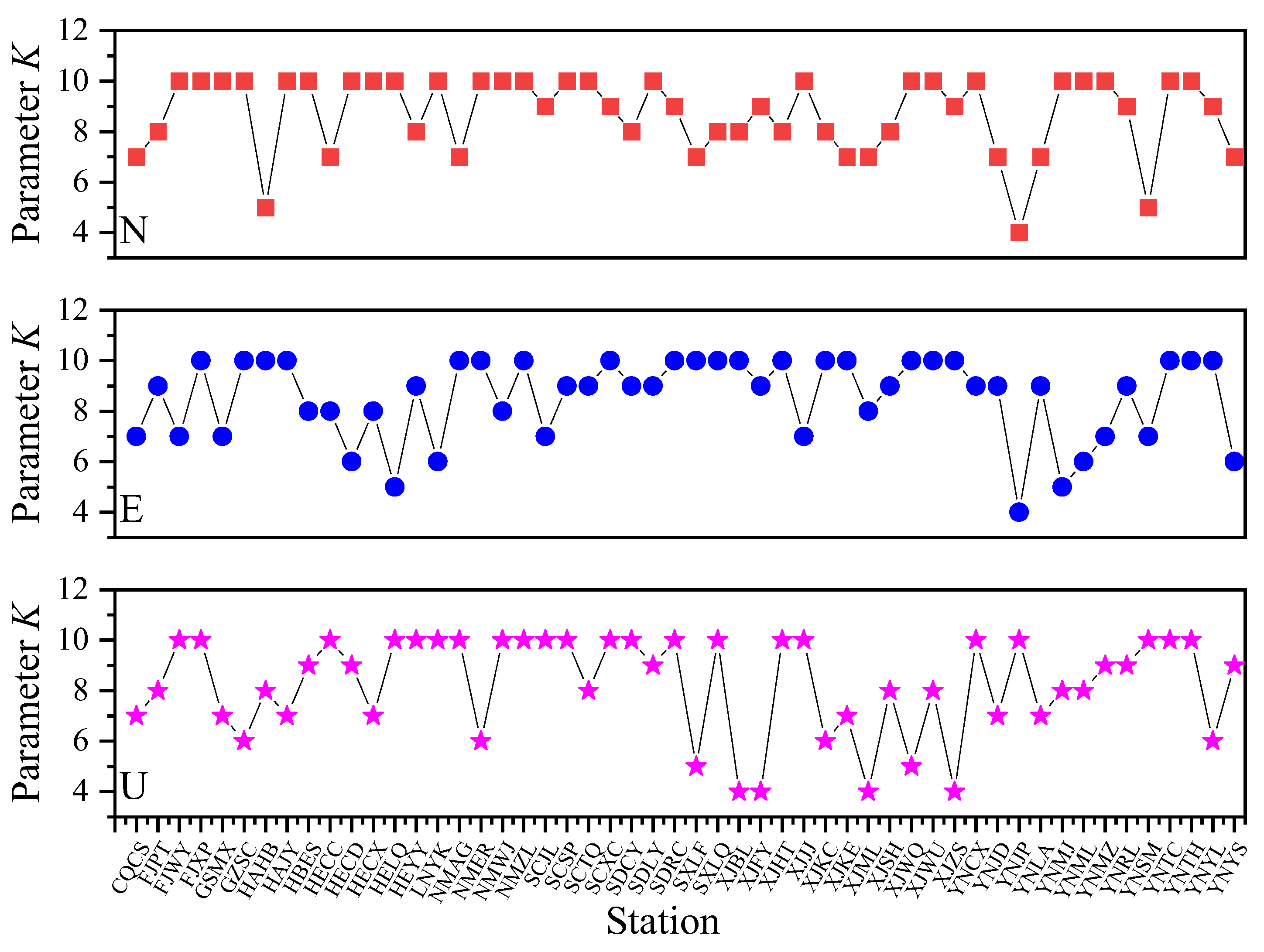
Figure 12.
Distribution of optimal parameter values for GNSS stations.
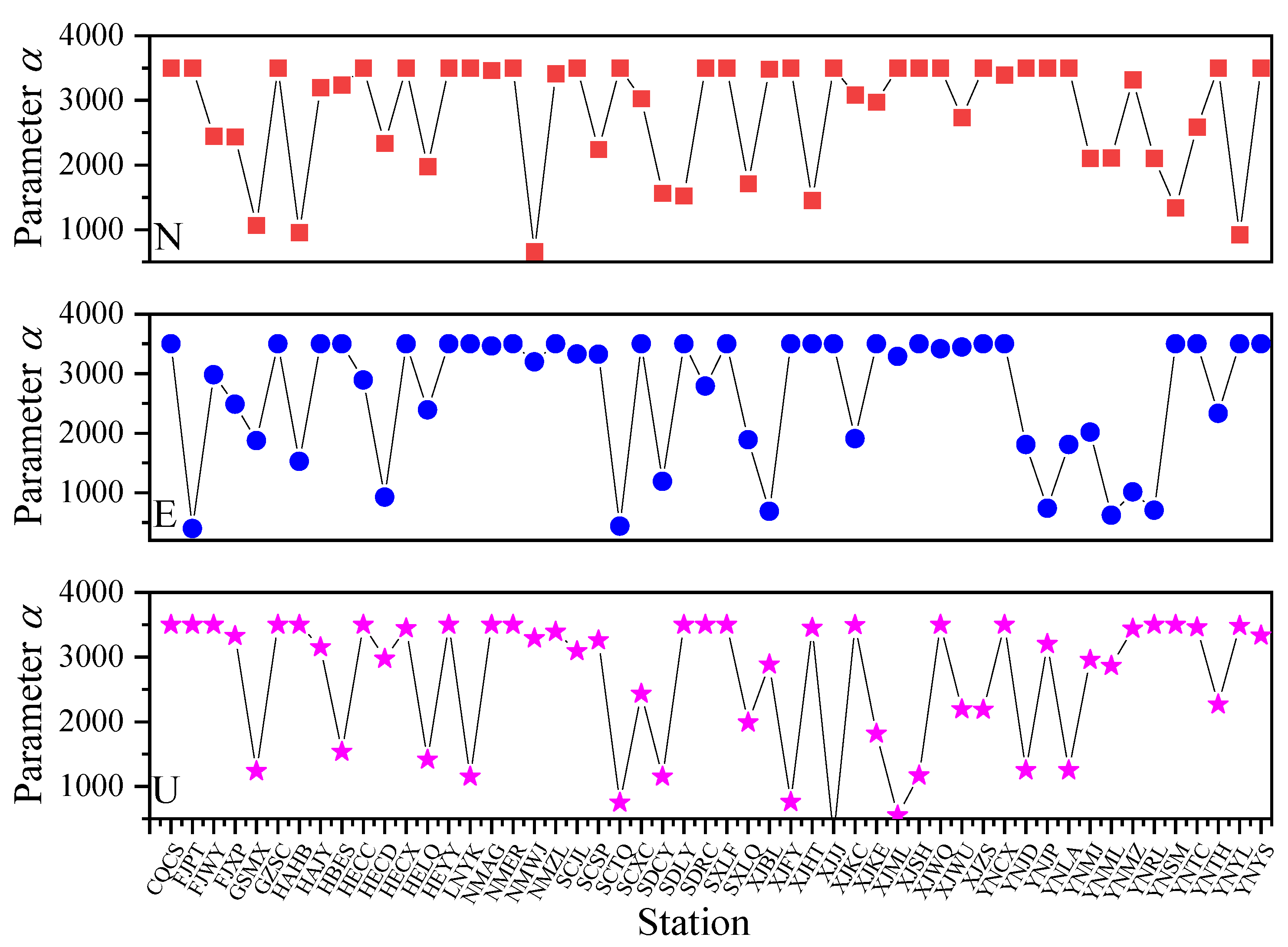
Figure 13.
Comparison of noise reduction effects in three directions of FJPT sites.
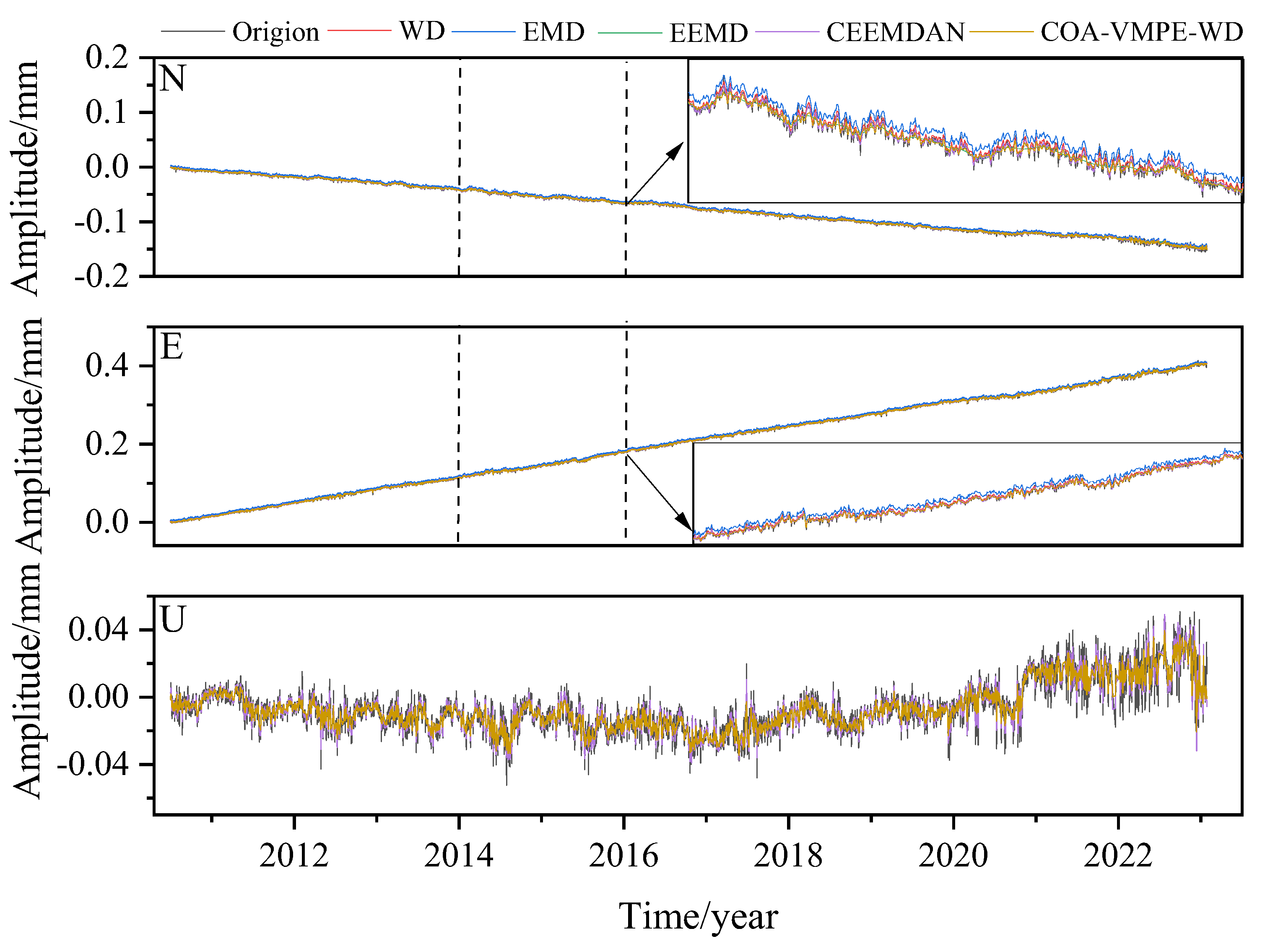
Figure 14.
Residual results between the denoised signal and the original reference signal.
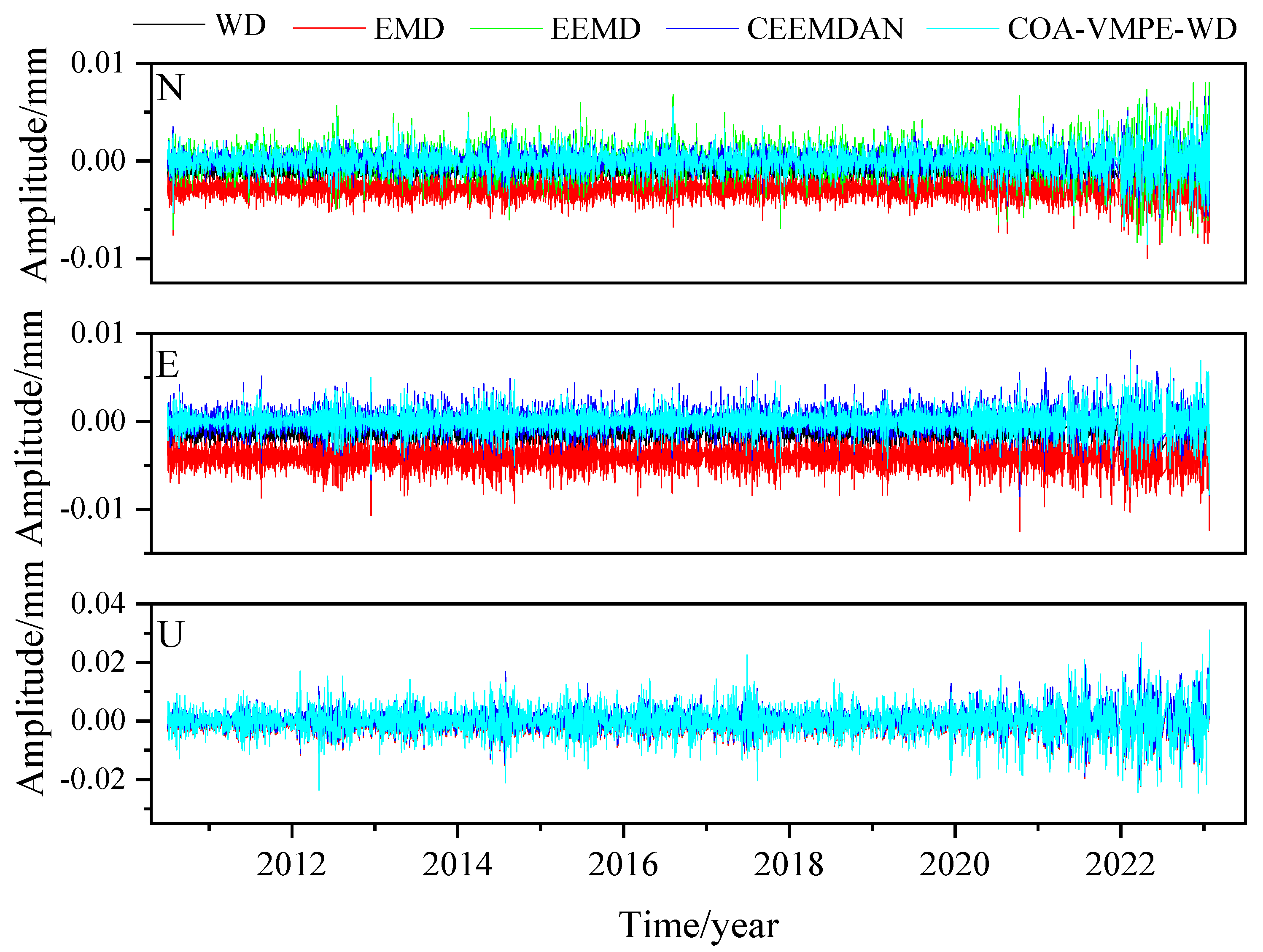
Figure 15.
Distribution of four evaluation indicators on the N-component.
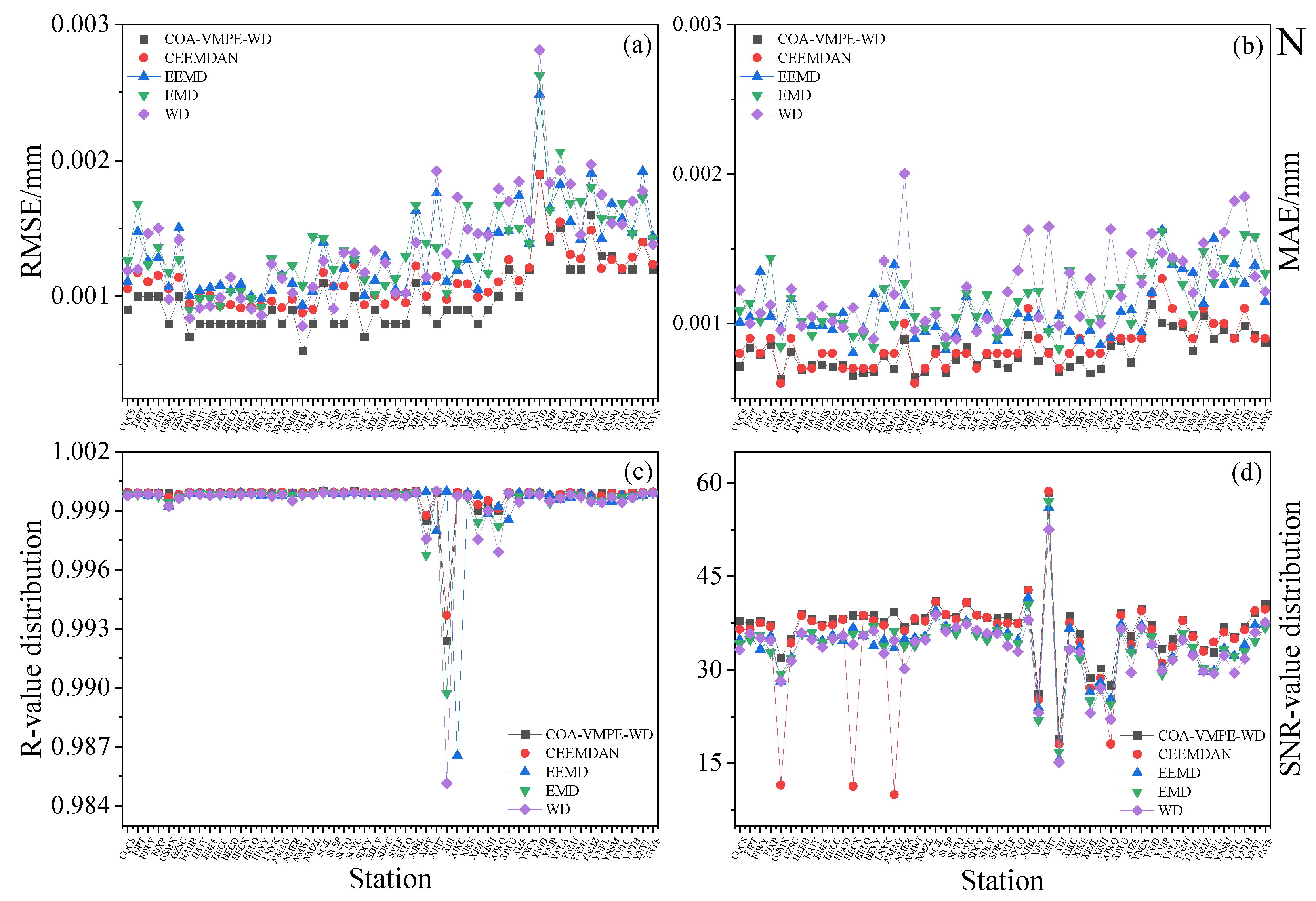
Figure 16.
Distribution of four evaluation indicators on the E-component.
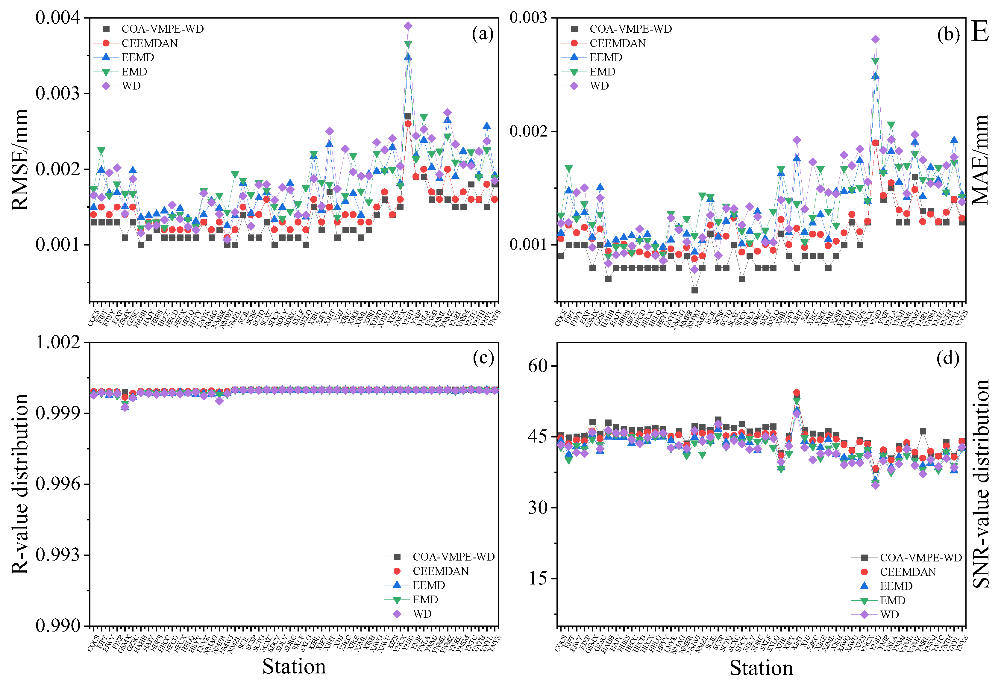
Figure 17.
Distribution of four evaluation indicators on the U-component.
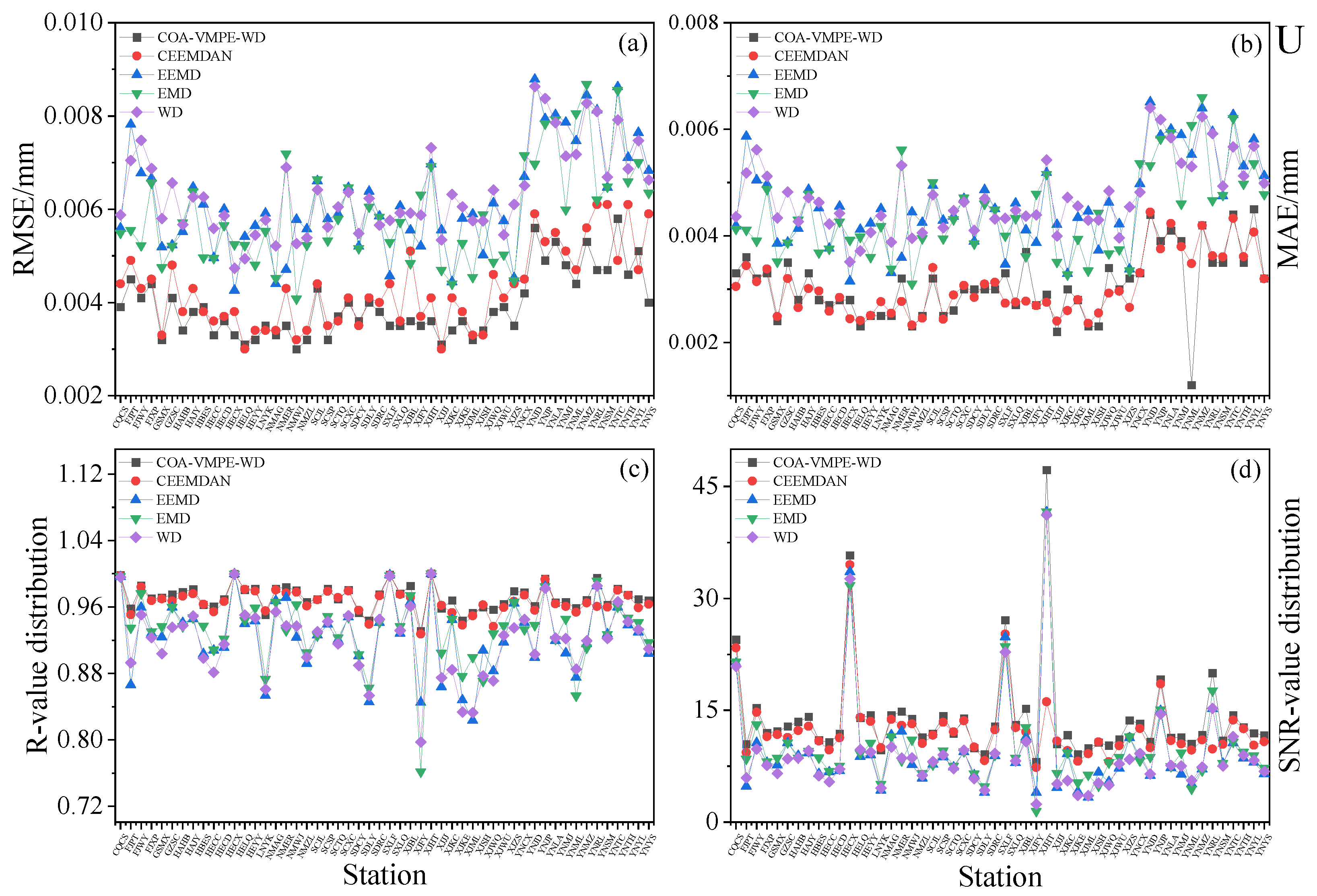
Figure 18.
Amplitude distribution under PLWN noise model for E, N, and U components.
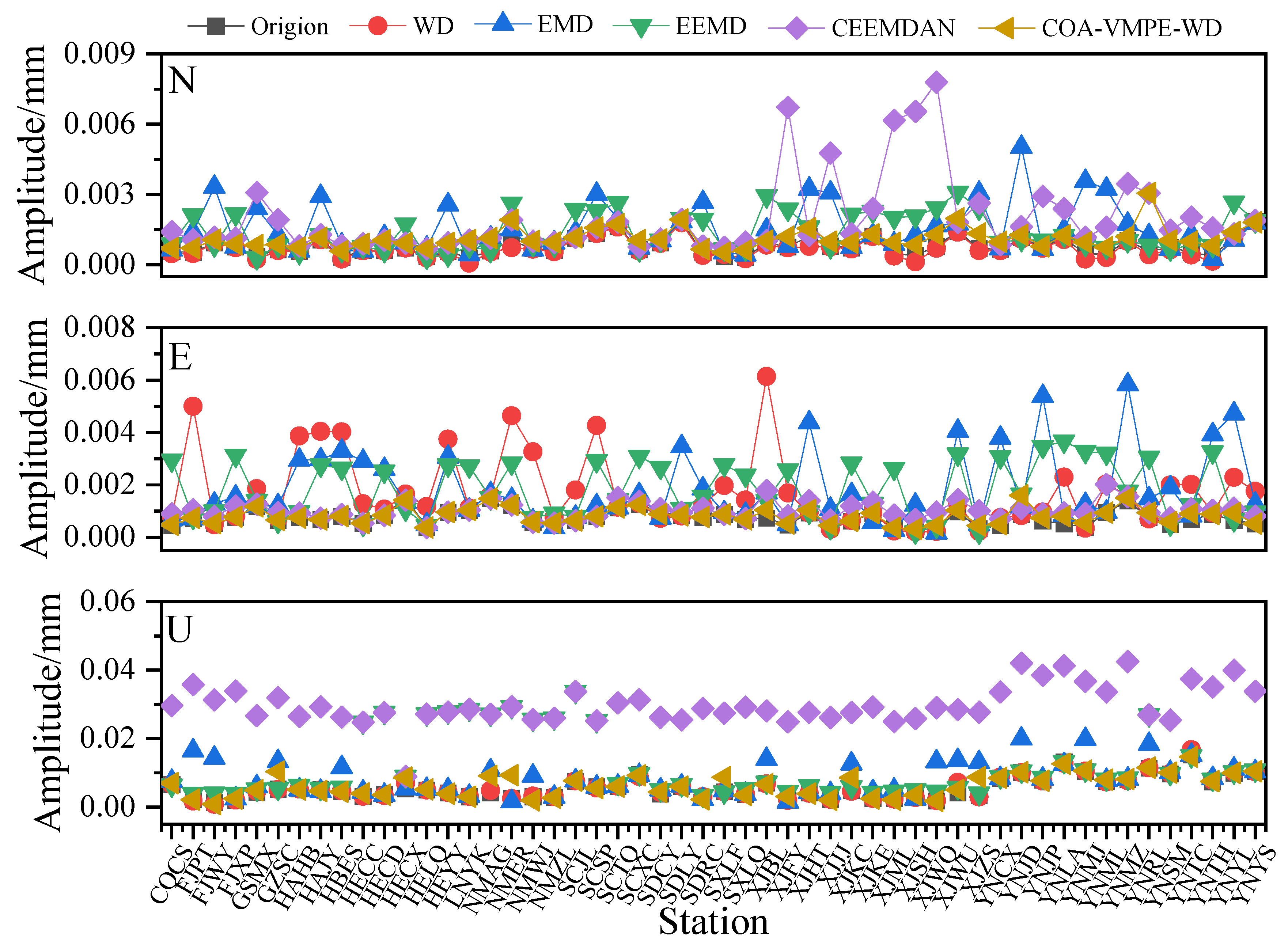
Figure 19.
Distribution of reference station velocity and station velocity uncertainty after denoising using different method.
Figure 19.
Distribution of reference station velocity and station velocity uncertainty after denoising using different method.
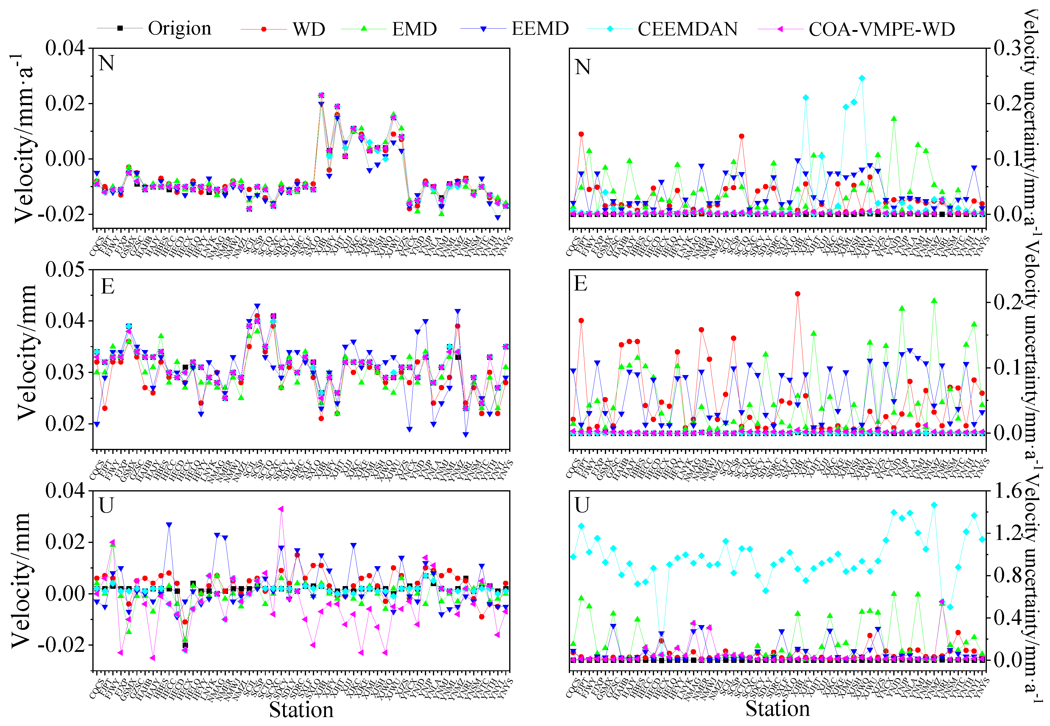

Table 1.
Mean MPE of each IMF component after COA-VMD decomposition.
| Modal component | IMF1 | IMF2 | IMF3 | IMF4 | IMF5 | IMF6 | IMF7 | IMF8 |
| MPE | 0.4059 | 0.6033 | 0.7113 | 0.7668 | 0.7955 | 0.8085 | 0.8113 | 0.8229 |
Table 2.
Noise Reduction Evaluation Indicators for four Methods of Simulating Signals.
| Noise reduction methods | Evaluation | |||
| RMSE/mm | SNR/dB | MAE/mm | R | |
| WD | 1.1971 | 12.8760 | 0.9734 | 0.8777 |
| EMD | 1.3119 | 25.1553 | 0.2329 | 0.9722 |
| EEMD | 1.2384 | 12.8041 | 0.9913 | 0.9300 |
| CEEMDAN | 1.2136 | 13.1049 | 1.0139 | 0.9145 |
| COA-VMPE-WD | 0.2291 | 27.8397 | 0.1780 | 0.9757 |
Table 3.
Optimal Noise Models for E, N, and U Components of 52 GNSS Stations.
| Station | N | E | U | Station | N | E | U |
| CQCS | PLWN | FNRWWN | FNWN | SXLF | FNWN | PLWN | FNWN |
| FJPT | PLWN | FNRWWN | FNRWWN | SXLQ | FNWN | PLWN | FNWN |
| FJWY | PLWN | FNRWWN | FNRWWN | XJBL | PLWN | PLWN | PLWN |
| FJXP | PLWN | FNWN | FNRWWN | XJFY | PLWN | FNWN | FNWN |
| GSMX | FNRWWN | FNRWWN | FNRWWN | XJHT | PLWN | FNWN | PLWN |
| GZSC | PLWN | FNWN | FNRWWN | XJJJ | PLWN | FNWN | FNWN |
| HAHB | FNWN | PLWN | FNRWWN | XJKC | PLWN | FNWN | FNRWWN |
| HAJY | FNWN | FNWN | FNWN | XJKE | PLWN | FNWN | FNWN |
| HBES | PLWN | PLWN | FNRWWN | XJML | PLWN | FNWN | FNWN |
| HECC | PLWN | PLWN | FNWN | XJSH | PLWN | FNWN | FNWN |
| HECD | PLWN | PLWN | FNWN | XJWQ | PLWN | FNWN | FNWN |
| HECX | PLWN | PLWN | FNRWWN | XJWU | PLWN | PLWN | PLWN |
| HELQ | PLWN | PLWN | FNWN | XJZS | PLWN | FNWN | FNWN |
| HEYY | PLWN | FNRWWN | FNWN | YNCX | PLWN | FNWN | FNRWWN |
| LNYK | FNWN | PLWN | FNWN | YNJD | PLWN | FNWN | FNRWWN |
| NMAG | PLWN | PLWN | FNWN | YNJP | PLWN | PLWN | FNRWWN |
| NMER | PLWN | PLWN | FNWN | YNLA | PLWN | PLWN | FNRWWN |
| NMWJ | PLWN | PLWN | FNWN | YNMJ | PLWN | FNWN | PLWN |
| NMZL | FNWN | PLWN | FNWN | YNML | PLWN | PLWN | FNRWWN |
| SCJL | FNRWWN | FNRWWN | PLWN | YNMZ | FNRWWN | FNWN | FNRWWN |
| SCSP | PLWN | FNRWWN | FNWN | YNRL | PLWN | PLWN | FNRWWN |
| SCTQ | FNRWWN | PLWN | FNWN | YNSM | FNRWWN | PLWN | PLWN |
| SCXC | PLWN | PLWN | PLWN | YNTC | PLWN | PLWN | FNRWWN |
| SDCY | PLWN | FNWN | FNWN | YNTH | FNWN | FNWN | PLWN |
| SDLY | PLWN | PLWN | FNWN | YNYL | PLWN | FNWN | FNRWWN |
| SDRC | PLWN | FNRWWN | FNWN | YNYS | PLWN | FNWN | FNWN |
Table 4.
Optimal Noise Model of GNSS Stations after Different Noise Reduction Methods.
| Component | Orgion | WD | EMD | EEMD | CEEMDAN | COA-VMPE-WD |
| N | PLWN | PLWN | PLWN | PLWN | PLWN FNRW |
PLWN FNRW |
| E | PLWN | PLWN | PLWN | PLWN | PLWN | PLWN |
| FNRWWN | PLWN | PLWN | PLWN | FNRWWN | FNRW | |
| U | FNRWWN | PLWN | PLWN | PLWN | PLWN | PLWN |
| FNWN | PLWN | PLWN | PLWN | PLWN | FNRW |
Table 5.
Absolute values of mean velocities of different components using different methods (mm/a).
| Component | Origin | WD | EMD | EEMD | CEEMDAN | COA-VMPE-WD |
| N | 0.018 | 0.018 | 0.020 | 0.021 | 0.018 | 0.010 |
| E | 0.023 | 0.021 | 0.022 | 0.023 | 0.023 | 0.018 |
| U | 0.022 | 0.018 | 0.022 | 0.011 | 0.025 | 0.009 |
Disclaimer/Publisher’s Note: The statements, opinions and data contained in all publications are solely those of the individual author(s) and contributor(s) and not of MDPI and/or the editor(s). MDPI and/or the editor(s) disclaim responsibility for any injury to people or property resulting from any ideas, methods, instructions or products referred to in the content. |
© 2025 by the authors. Licensee MDPI, Basel, Switzerland. This article is an open access article distributed under the terms and conditions of the Creative Commons Attribution (CC BY) license (http://creativecommons.org/licenses/by/4.0/).
Copyright: This open access article is published under a Creative Commons CC BY 4.0 license, which permit the free download, distribution, and reuse, provided that the author and preprint are cited in any reuse.


