
Submitted:
13 August 2025
Posted:
13 August 2025
You are already at the latest version
Abstract
This research used a 124-year historical record of monthly rainfall col- lected on the Santa Eliza farm at the Instituto Agronômico de Campinas in southeastern Brazil. The methodology employed was to conduct a chi- square test in 30- and 10-year increments and compare the four and twelve periods that comprised the total of the analyzed series from 1890 to 2014. As a result of the chi-square test, there is no statistical evidence that its variability exhibited trends, allowing one to conclude that the frequency variability of maximum rainfall exhibits random variability, falling within the range of natural variability.
Keywords:
long-term time series
; chi-square test
; climate variability
; extreme rainfall
; natural climate variability
1. Introduction
A constant search to analyze and record significant changes in maximum rainfall in southeastern Brazil, due to its strategic importance in the national economy and industry. Therefore, it is important to use long-term time series with high-quality records. However, few institutions maintain such datasets. Relevant long-term data are often available only from large urban centers, where measurements over time have been influenced by the presence of urban heat islands, thereby affecting recent climatological averages. The terrestrial planetary system is composed of very complex systems with different temporal scales, different response times, and overlapping physical scales that result in behaviors that modulate multidecadal and intradecadal dynamics. Byshev et al. (2022) showed that a specific feature of the current climate dynamics consists of its multidecadal oscillations with a period of about 20 to 60 years and intradecadal disturbances with time scales of 2 to 8 years. A certain globality and near-synchronism of multidecadal climate changes occur involving planetary thermodynamic structures in the two most important components of the climate system, namely the ocean and the atmosphere. A multidecadal variability signal response at the planetary level is an extremely complex dynamic structure because solar activity acts in the stratosphere and creates circulation patterns that characterize the Brewer-Dobson circulation in the tropical region. Iglesias-Suarez et al. (2021) noted in their result that there is observational and modeling evidence suggesting that the recent acceleration of the Brewer-Dobson stratospheric circulation would be driven by climate change and stratospheric ozone depletion. However, the naturally occurring, slowly varying variability may compromise our ability to detect such forced changes in a relatively short observational record. Using observations and chemical-climatic model simulations, they demonstrated that there is a link between multidecadal variability in Brewer-Dobson circulation alteration and the Pacific Interdecadal Oscillation, with indirect impacts on composition in the stratosphere. In this aspect, it helps influence the behavior of the lower stratosphere by influencing the models of circulation in the troposphere. It could seek to analyze climatic indices and associate them with solar activity in a significant way. Correa et al. (2019) used the R statistical software with the WaveletComp package to generate the Morlet wavelet power spectra and bivariate analysis with cross-wavelet and the biwavelet package. As a result, signals with dominant cycles were obtained, and variability of the order of 32, 64, 128, and 256 months was observed, with 2.66, 5.33, 10.66, and 21.33 years. These are observed in the variability of the period from January 1933 to September 2016, in a total of 993 months (82.75 years), characterized by decadal to multidecadal variations. These observed multidecadal cycles (between 10.66 and 21.33 years) may have some correlation with the variability of solar activity (sunspots) and the cycles of climate variability in the atmospheric/ocean system. Corrêa et al. (2022) used a long historical series (70 years) in southeastern Brazil and observed that the oscillation frequencies of maximum values equal to or greater than 180 and 300 mm of rain did not show changes in the maximum frequencies of rainfall intensity. This implies that the multidecadal variability is within the natural variability of large dynamic systems, showing random variability. It also concludes, in non-parametric statistical tests, that it is within the limits of randomness for at least the last 70 years, without characterizing trends in the analyzed time series. By definition, climate phenomena on the zonal scale have horizontal extension between 1000 and 5000 kilometers and vertically embrace the entire atmosphere. Also, to define a periodicity, the records necessary to understand climates on the zonal scale must be obtained at the level of the climatological norm, with minimum periods of observations of 30 years. Climate variability calculated by the 30-year normal can be interpreted as the true state of background that compensates for the effects of the decadal and long-term trend and the associated annual variability, as well as random fluctuations and systematic errors, assuming a stationary level that is the zonal scale level. Therefore, the use of a 30-year normal series is defined by the World Meteorological Organization (2017). When we use periods under 30 years, we are adding instability because the use of climatological media is variable in conservative synthesis, assuming a degree of stationarity. The use of periods of 10 and 5 years would implicitly induce influences of smaller temporal-scale systems. It is rare to analyze long-time series with technical quality in observation. The purpose of this study is to examine a meteorological station in southeastern Brazil over a long time series (124 years) to see if there was a change in the maximum frequencies of monthly precipitation at statistical significance levels of 5% and 1%, as well as whether rainfall maximums are within natural variability or if intradecadal and multidecadal trends exist.
2. Methodology
2.1. Monthly Climate Time Series
This analysis uses monthly rainfall data collected at the Centro Experimental de Campinas (CEC), located on the Santa Eliza farm of the Instituto Agronômico de Campinas (IAC). One of the problems with analyzing observational data is the lack of long and reliable time series and poor observation quality. The series collected at the IAC is excellent because, in addition to being over 124 years old, it reflects the quality of the work and dedication of its institution, as the meteorological information collection station was located in a farm area. This information is not directly influenced by an increase in observation or a thermal island in large urban centers. Such situations can influence rainfall regimes. Figure 1 shows the dispersion of the monthly rainfall data from the IAC. The data dispersion can be represented by the interquartile range, which is the difference between the third quartile and the first quartile. The interquartile range is the most robust statistic to measure variability since it is not influenced by outliers. The first quartile (Q1) is the base of the rectangular gray box. A demarcation that distinguishes that 25% of the data is below and the other 75% of the data is above this value. Median or second quartile (Q2)—the line is more to the center of the gray rectangular box to demarcate the central value of the database. 50% of the data is higher than this value, and the other 50% of the data is lower. Third Quartile (Q3)—the top of the rectangular box. This line informs the number that is between 75% lower values and 25% higher values. The maximum value of the data set is the circles above the upper horizontal line, but respecting a calculated limit. It is possible to exist above this in the Outliers database.
2.2. Non-Parametric Chi-Squared Test
The chi-square test can be used involving only the observed frequency (Spiegel and Stephens, 2008; Thompson, 1988). To carry out this frequency estimate, the maximum values obtained by the cluster analysis technique of the monthly precipitation time series are used; for southeastern Brazil, whose maximum value was used as a reference, the most frequent value in the series was 180 mm (Correa et al., 2022). The occurrence of rainfall for frequency values equal to or greater than 180 mm and greater than 300 mm will be calculated. It is considered that the frequencies of maximum precipitation are exclusive and independent. Contingency tables of 2 x 2 will be used (Table 1). The series will be divided into periods of 30 and 10 years each and will analyze the chi-square test over 124 years to compare the periods between 1890 and 2014.
Where , , , , , and , this becomes:
The values obtained will be tested at 1 degree of freedom at a 5% level and a 1% level of significance with the following hypotheses: critical values for the test for a degree of freedom correspond to 6.63 (1%) and 3.84 (5%), Sheskin (2004):
- = It is true if the variables are random; the monthly maximum values of precipitation have random variability.
- = It is true if the variables are not random and the monthly maximum values of precipitation will have trends.
2.3. Statistical Methods
To evaluate the uniformity and independence of precipitation events across time intervals, we applied a non-parametric permutation test, which is particularly suitable for count data and does not rely on large-sample or distributional assumptions.
The test statistic used was the classical Pearson’s chi-square, calculated for the observed frequency distribution of monthly events with precipitation mm across the 12 decadal periods. To assess the significance of the observed statistic, we generated 10,000 randomized datasets under the null hypothesis of a uniform distribution, using multinomial sampling with equal probabilities for each period. For each permutation, the chi-square statistic was recalculated.
The empirical p-value was estimated as the proportion of permuted statistics greater than or equal to the observed value. This approach ensures a robust assessment of randomness and allows us to evaluate whether the observed deviations could plausibly arise by chance alone.
3. Result
Table 2 shows the maximum rainfall frequencies in 30-year periods in an interval of 120 years from 1890 to 2009. The 30-year periods varied in frequency from 300 mm with variability from 17 to 23 times and from 180 mm between 61 and 70 times, with 70 times in the period from 1980 to 2009 being the last period.
It is important to clarify that the intermediate precipitation class, denoted as mm, refers to the interval , which represents the maximum monthly precipitation observed within this range.
Table 3 presents the results of the chi-square test calculated at the 5% and 1% significance levels, compared to the tabulated chi-square values. In none of the comparisons was the calculated value greater than the critical threshold, indicating that there is no statistical evidence to reject the null hypothesis . Therefore, the data are compatible with the hypothesis of randomness, and the observed frequencies fall within the range of natural climatic variability, without evidence of a trend.
The values in Table 4 confirm that there is no statistical indication of a trend across the 30-year periods. This leads us to accept the null hypothesis , implying that the time series of monthly precipitation recorded at the IAC over the past 120 years does not show significant changes in the frequency of maximum precipitation events exceeding 180 mm and 300 mm.
In Table 5, there were six instances in which the calculated chi-square values exceeded the 5% significance threshold. However, at the more stringent 1% level, none of the values surpassed the critical chi-square value of 6.63.
It is worth noting that, a priori, the largest differences in maximum monthly precipitation frequencies appeared in the earlier decades of the dataset, particularly in the 1900s and 1920s. The distribution of monthly events with precipitation mm over the 12 decadal periods did not exhibit any statistically significant deviation from a uniform distribution (, ), as confirmed by the theoretical chi-square test using scipy.stats.chisquare ().
This finding was corroborated by both the parametric chi-square test and a randomization procedure with 10,000 permutations. This suggests that the observed variations in frequency can be attributed to chance, and that the statistical test supports the assumption of randomness in the occurrence of extreme precipitation events.
4. Conclusions
The use of the chi-square test allowed us to verify, with statistical reliability, that the maximum precipitation frequencies do not change, which characterizes that the maxima are within the natural climatic variability, which were observed in the agricultural region of Santa Eliza, in the IAC, Campinas, Southeast of Brazil. Complementary analyses were performed over 5 years, which maintained the same randomness results. The results show the consistency of the scale analyses (10 and 30 years), which strengthens the conclusion of random variability in the analyzed period. The frequency values in maximum events in 30 and 10 years in a total series of 124 years are within the statistical variation of randomness without presenting trends. Based on the analysis of the chi-square test, we cannot affirm that there is a trend in the time series of monthly maximum precipitation. This allows us to conclude that the maximum precipitation frequencies are associated with random global dynamic mechanisms. The series is qualified and continuous. Currently, there are few series that can be used for this type of analysis because they present metadata records or observation history for the time series.
References
- ANGEL, J. R., EASTERLING, W. E., & KIRSCH, S. W. (1993). Towards defining appropriate averaging periods for climate normals. Climatological Bulletin, 27(2), 29–44.
- ARGUEZ, A., & VOSE, R. S. (2011). The definition of the standard WMO climate normal: The key to deriving alternative climate normals. Bulletin of the American Meteorological Society, 92(6), 699–704. [CrossRef]
- BARROS, H. R., & LOMBARDO, M. A. (2016). A ilha de calor urbana e o uso e cobertura do solo no município de São Paulo-SP. GEOUSP Espaço e Tempo (Online), 20(1), 160–177.
- BYSHEV, V., GUSEV, A., NEIMAN, V., & SIDOROVA, A. (2022). Interdecadal Oscillation of the Ocean Heat Content. Journal of Marine Science and Engineering, 10(8), 1064. [CrossRef]
- BUTCHART, N. (2014). The Brewer-Dobson circulation. Reviews of Geophysics, 52(2), 157–184. [CrossRef]
- CORRÊA, C. S., GUEDES, R. L., CORRÊA, K. A. B., & PILAU, F. G. (2019). Multidecadal cycles in climate indexes using wavelet analysis. Anuário do Instituto de Geociências, 42(1), 66–73.
- CORRÊA, C. S., de QUEIROZ, A. P., CORRÊA, K. A. B., & MARTIN, I. M. (2022). Monthly Precipitation in Southeast Brazil. Latin American Journal of Development, 4(5), 1670–1683. [CrossRef]
- HARDIMAN, S. C., LIN, P., SCAIFE, A. A., DUNSTONE, N. J., & REN, H. L. (2017). Dynamical variability and the Brewer-Dobson trend. Geophysical Research Letters, 44(6), 2885–2892.
- IGLESIAS-SUAREZ, F., et al. (2021). Tropical Stratospheric Circulation and Pacific Multi-Decadal Variability. Geophysical Research Letters, 48(11), e2020GL092162. [CrossRef]
- MARCHI, M., et al. (2020). Climate EU: climate normals and projections. Scientific Data, 7(1), 428. [CrossRef]
- NAIKOO, M. W., et al. (2022). Land cover change and urban heat islands. Urban Climate, 41, 101052. [CrossRef]
- PLOEGERL, F., & GARNY, H. (2022). Asymmetries in stratospheric circulation. Atmospheric Chemistry and Physics, 22(8), 5559–5576. [CrossRef]
- RIBEIRO, A. G. (1993). As escalas do clima. Boletim de Geografia Teorética, 23(45-46), 288–294.
- ROMERO, M. A. B., et al. (2019). Mudanças climáticas e ilhas de calor urbanas.
- SHESKIN, D. (2004). Handbook of parametric and nonparametric statistical procedures. Chapman & Hall CRC.
- SPIGEL, M. R., & STEPHENS, L. J. (2008). Statistics – Schaum’s Outlines. McGraw-Hill.
- THOMPSON, B. (1988). Misuse of chi-square statistics. Educational and Psychological Research, 8(1), 39–49.
- WEBER, M., et al. (2011). The Brewer-Dobson circulation and ozone. Atmospheric Chemistry and Physics, 11(21), 11221–11235. [CrossRef]
- WON, S. J., WANG, X. H., & WARREN, H. E. (2016). Climate normals for utility regulation. Energy Economics, 54, 405–416. [CrossRef]
- WORLD METEOROLOGICAL ORGANIZATION. (2017). WMO guidelines on the calculation of climate normals.
Figure 1.
Boxplot of monthly rainfall (mm) time series (1890-2009) from the IAC station in Campinas, SP.
Figure 1.
Boxplot of monthly rainfall (mm) time series (1890-2009) from the IAC station in Campinas, SP.
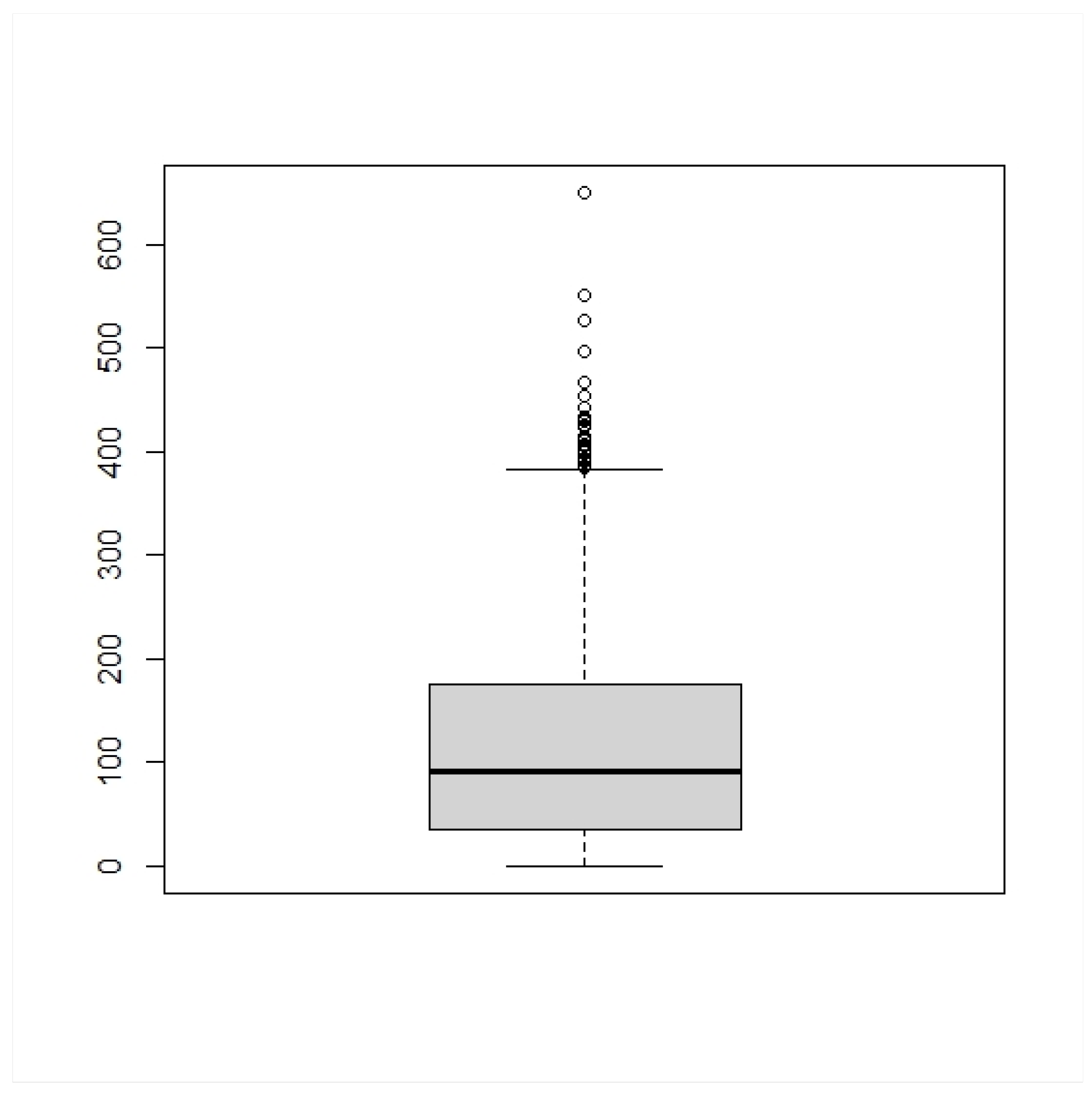

Table 1.
Contingency tables of 2 x 2.
| ≥ 300 mm | ≥ 180 mm | TOTAL | |
|---|---|---|---|
| 30 years of rainfall period | |||
| 30 years of rainfall period | |||
| TOTAL | N |
Table 2.
Frequency of monthly precipitation maximums in 124 years, divided into 4, 12 e 25 periods for calculating the chi-square test, from 1890 to 2014.
Table 2.
Frequency of monthly precipitation maximums in 124 years, divided into 4, 12 e 25 periods for calculating the chi-square test, from 1890 to 2014.
| 30 years | ≥ 300 mm | ≥ 180 mm | 10 years | ≥ 300 mm | ≥ 180 mm |
|---|---|---|---|---|---|
| 1º | 21 | 66 | 1º | 12 | 23 |
| 2º | 23 | 63 | 2º | 7 | 19 |
| 3º | 17 | 61 | 3º | 2 | 24 |
| 4º | 20 | 70 | 4º | 8 | 25 |
| 5º | 10 | 20 | |||
| 6º | 5 | 18 | |||
| 7º | 4 | 21 | |||
| 8º | 7 | 24 | |||
| 9º | 6 | 16 | |||
| 10º | 3 | 28 | |||
| 11º | 10 | 19 | |||
| 12º | 7 | 23 |
Table 3.
The monthly rainfall occurrence of the frequency values is equal to or greater than 180 and 300 mm.
Table 3.
The monthly rainfall occurrence of the frequency values is equal to or greater than 180 and 300 mm.
| 1º x 2º | ≥300 mm | ≥180mm | total | 2º x 3º | ≥300 mm | ≥180mm | total |
|---|---|---|---|---|---|---|---|
| 1890-1919 | 21 | 66 | 87 | 1920-1949 | 23 | 63 | 86 |
| 1920-1949 | 23 | 63 | 86 | 1950-1979 | 17 | 61 | 78 |
| total | 44 | 129 | 173 | total | 40 | 124 | 164 |
| 3º x 4º | ≥300 mm | ≥180mm | total | 1º x 3º | ≥300 mm | ≥180mm | total |
| 1950-1979 | 17 | 61 | 78 | 1890-1919 | 21 | 66 | 87 |
| 1980-2009 | 20 | 70 | 90 | 1950-1979 | 17 | 61 | 78 |
| total | 37 | 131 | 168 | total | 38 | 127 | 165 |
| 1º x 4º | ≥300 mm | ≥180mm | total | 2º x 4º | ≥300 mm | ≥180mm | total |
| 1890-1919 | 21 | 66 | 87 | 1920-1949 | 23 | 63 | 86 |
| 1980-2009 | 20 | 70 | 90 | 1980-2009 | 20 | 70 | 90 |
| total | 41 | 136 | 177 | total | 43 | 133 | 176 |
Table 4.
Chi-squared test results for a degree of freedom corresponding to 1% and 5%, in periods of 30 years.
Table 4.
Chi-squared test results for a degree of freedom corresponding to 1% and 5%, in periods of 30 years.
| 1º x 2º | Tabulated | Calculated value | 2º x 3º | Tabulated | Calculated value |
|---|---|---|---|---|---|
| 5% | 3.84 | 0.1549 | 5% | 3.84 | 0.5433 |
| 1% | 6.63 | 1% | 6.63 | ||
| 3º x 4º | Tabulated | Calculated value | 1º x 3º | Tabulated | Calculated value |
| 5% | 3.84 | 0.0044 | 5% | 3.84 | 0.1273 |
| 1% | 6.63 | 1% | 6.63 | ||
| 1º x 4º | Tabulated | Calculated value | 2º x 4º | Tabulated | Calculated value |
| 5% | 3.84 | 0.0912 | 5% | 3.84 | 0.4870 |
| 1% | 6.63 | 1% | 6.63 |
Table 5.
Chi-squared test result for a degree of freedom, in periods of 10 years, calculated values. Tabulated Chi-squared 5% level (3.84) and 1% level (6.63).
Table 5.
Chi-squared test result for a degree of freedom, in periods of 10 years, calculated values. Tabulated Chi-squared 5% level (3.84) and 1% level (6.63).
| 1º x 2º | 0.3770 | ||||||
|---|---|---|---|---|---|---|---|
| 1º x 3º | 5.9661 | 2º x 3º | 3.3591 | ||||
| 1º x 4º | 0.8252 | 2º x 4º | 0.0551 | 3º x 4º | 2.8297 | ||
| 1º x 5º | 0.0065 | 2º x 5º | 0.2707 | 3º x 5º | 5.4390 | 4º x 5º | 0.6363 |
| 1º x 6º | 1.0544 | 2º x 6º | 0.1773 | 3º x 6º | 1.9665 | 4º x 6º | 0.0476 |
| 1º x 7º | 2.4935 | 2º x 7º | 0.8989 | 3º x 7º | 0.8473 | 4º x 7º | 0.5889 |
| 1º x 8º | 1.0986 | 2º x 8º | 0.1439 | 3º x 8º | 2.3573 | 4º x 8º | 0.0245 |
| 1º x 9º | 0.3074 | 2º x 9º | 0.0010 | 3º x 9º | 3.2895 | 4º x 9º | 0.0638 |
| 1º x 10º | 5.6685 | 2º x 10º | 2.9071 | 3º x 10º | 0.0696 | 4º x 10º | 2.3823 |
| 1º x 11º | 0.0002 | 2º x 11º | 0.3668 | 3º x 11º | 5.7682 | 4º x 11º | 0.7856 |
| 1º x 12º | 0.9367 | 2º x 12º | 0.0957 | 3º x 12º | 2.5262 | 4º x 12º | 0.0075 |
| 5º x 6º | 0.8624 | ||||||
| 5º x 7º | 2.1591 | 6º x 7º | 0.2589 | ||||
| 5º x 8º | 0.8768 | 6º x 8º | 0.0054 | 7º x 8º | 0.3796 | ||
| 5º x 9º | 0.2188 | 6º x 9º | 0.1864 | 7º x 9º | 0.8878 | 8º x 9º | 0.1530 |
| 5º x 10º | 5.0875 | 6º x 10º | 1.5221 | 7º x 10º | 0.5058 | 8º x 10º | 1.9076 |
| 5º x 11º | 0.0086 | 6º x 11º | 1.0148 | 7º x 11º | 2.3882 | 8º x 11º | 1.0453 |
| 5º x 12º | 0.7387 | 6º x 12º | 0.0188 | 7º x 12º | 0.4583 | 8º x 12º | 0.0574 |
| 9º x 10º | 2.8259 | ||||||
| 9º x 11º | 0.3020 | 10º x 11º | 5.4320 | ||||
| 9º x 12º | 0.1050 | 10º x 12º | 2.0743 | 11º x 12º | 0.8936 |
Disclaimer/Publisher’s Note: The statements, opinions and data contained in all publications are solely those of the individual author(s) and contributor(s) and not of MDPI and/or the editor(s). MDPI and/or the editor(s) disclaim responsibility for any injury to people or property resulting from any ideas, methods, instructions or products referred to in the content. |
© 2025 by the authors. Licensee MDPI, Basel, Switzerland. This article is an open access article distributed under the terms and conditions of the Creative Commons Attribution (CC BY) license (http://creativecommons.org/licenses/by/4.0/).
Copyright: This open access article is published under a Creative Commons CC BY 4.0 license, which permit the free download, distribution, and reuse, provided that the author and preprint are cited in any reuse.


