
Submitted:
12 August 2025
Posted:
13 August 2025
You are already at the latest version
Abstract
Frame Replication and Elimination for Reliability (FRER) in Time-Sensitive Networking (TSN) enhances fault tolerance by duplicating critical traffic across disjoint paths. However, always-on FRER configurations impose constant redundancy overhead, even under nominal network conditions. This paper proposes a predictive FRER activation framework that leverages KPI-driven fault anticipation using a bidirectional Long Short-Term Memory (BiLSTM) model. By continuously analyzing multivariate performance indicators such as latency, jitter, and retransmission rates, the model forecasts impending faults and proactively triggers FRER. Redundancy is deactivated upon KPI recovery or after a minimum protection window, minimizing bandwidth consumption without compromising reliability. The framework includes a Python-based simulation environment, a real-time Streamlit dashboard for visualization, and a fully integrated runtime controller. Experimental results demonstrate significant improvements in link utilization while maintaining protection guarantees, showing the effectiveness of anticipatory redundancy strategies in industrial TSN environments.
Keywords:
time-sensitive networking
; FRER
; fault prediction
; industrial networks
; network reliability
1. Introduction
Industrial communication systems increasingly rely on deterministic Ethernet technologies to support real-time control, safety-critical operations, and ultra-reliable data delivery. Time-Sensitive Networking (TSN), standardized under the IEEE 802.1 suite [1], provides foundational mechanisms to ensure bounded latency, low jitter, and fault tolerance. Among these, Frame Replication and Elimination for Reliability (FRER), defined in IEEE 802.1CB [2], is a key component for enhancing communication robustness against transient link failures, device faults, or localized congestion [3].
FRER enhances reliability by duplicating frames across disjoint network paths, allowing receiving endpoints to eliminate duplicates and reconstruct the original traffic stream . This mechanism is particularly beneficial for critical data flows [4], where packet loss could compromise physical processes or pose operational hazards. In industrial deployments, FRER is often statically configured—either on a per-stream basis or network-wide—to provide consistent protection regardless of current network conditions.
However, static activation introduces a fundamental trade-off: while it ensures fault tolerance, it imposes constant redundancy overhead. Redundant transmissions consume additional bandwidth, increase network load, and may exacerbate congestion during peak periods [5]. In environments where network faults are rare or transient, always-on FRER leads to inefficient resource utilization. As industrial networks evolve to support dynamic, high-density workloads—including wireless TSN extensions [6]—this inefficiency becomes increasingly significant.
To address this, there is a growing need for adaptive FRER control aligned with real-time network conditions [7]. Although prior work has explored enhancements such as dynamic path selection, software-defined implementations, and integration with wireless domains, FRER activation remains largely decoupled from network observability and data-driven insights.
Recent advances in machine learning (ML), particularly in temporal modeling, offer a promising alternative. Time-series learning models can anticipate faults by identifying degradation patterns before service disruptions occur [8]. When tightly coupled with redundancy control, such predictive capabilities enable a new class of resilience strategies: anticipatory protection.
This paper presents a complete fault anticipation framework for predictive FRER activation in TSN-enabled industrial networks. The system monitors multivariate network performance indicators and applies a bidirectional Long Short-Term Memory (BiLSTM) model to forecast the likelihood of imminent faults. FRER is selectively enabled for affected streams when the predicted fault score exceeds a dynamic threshold, and deactivated upon KPI recovery or timeout expiry. This approach ensures redundancy is applied only during risk windows, minimizing bandwidth overhead without compromising reliability.
To validate our approach, we develop a runtime simulation and visualization environment that integrates the BiLSTM model, FRER activation logic, and a real-time Streamlit dashboard. Experimental results demonstrate the benefits of anticipatory redundancy in terms of link utilization, activation accuracy, and fault coverage.
The main contributions of this work are as follows:
- A synthetic KPI-based dataset generation pipeline tailored for modeling temporal degradation in TSN networks.
- A bidirectional LSTM model that accurately anticipates faults using time-series KPIs.
- A predictive FRER activation and deactivation mechanism integrated with the BiLSTM inference output.
- A complete runtime environment including a simulator and real-time dashboard for system state visualization and performance evaluation.
- A comprehensive evaluation of the framework in terms of redundancy efficiency, fault anticipation accuracy, and link utilization improvement.
2. Related Work
The intersection of reliability mechanisms in TSN and data-driven fault management has attracted considerable research attention across both industrial networking and machine learning domains. Prior work has extensively explored static and dynamic implementations of FRER, simulation-based performance analysis, and enhancements for edge and wireless deployments. In parallel, a growing body of literature investigates machine learning techniques for fault detection, prediction, and network observability in industrial environments [9,10,11,12,13,14]. While these research threads have matured independently, their integration remains limited. Specifically, no existing studies fully close the control loop by using predictive fault insights to drive real-time activation of TSN reliability mechanisms such as FRER. This section reviews the relevant literature in three categories: (i) FRER deployment and optimization, (ii) ML-based fault prediction in industrial networks, and (iii) ML applications within TSN systems.
2.1. Frame Replication and Elimination for Reliability in TSN
FRER is a core mechanism in TSN, standardized under IEEE 802.1CB [2], designed to ensure ultra-reliable communication in deterministic Ethernet networks. By replicating frames across disjoint paths and enabling receivers to discard duplicates using sequence identifiers, FRER facilitates seamless data recovery in the presence of link failures, transmission errors, or localized congestion. This makes it particularly valuable for safety-critical and time-sensitive industrial applications.
Amendments to the base standard, including IEEE 802.1CBcv and IEEE 802.1CBdb [15,16], ave introduced YANG-based management models and extended stream identification capabilities, enhancing the configurability and scalability of FRER deployments in modern industrial networks, including software-defined and virtualized environments.
To support analysis and benchmarking, simulation-based implementations of FRER have been developed using OMNeT++ and the INET framework. Danielis et al. [17] presented one such study, demonstrating FRER’s effectiveness in masking link-level failures, while also highlighting the persistent overhead associated with always-on redundancy under nominal conditions. Similar observations were reported by Maile et al. [4], who emphasized the need for runtime configurability to avoid excessive memory usage and frame reordering issues stemming from static buffer and sequence number settings.
Recent research has extended FRER to edge-cloud and wireless-integrated scenarios. Li et al. [7] proposed an optimized FRER scheme for edge computing networks, reducing overhead while maintaining resilience under burst-error conditions. Similarly, Aijaz et al. introduced X-FRER [18], a cross-domain extension for 5G-TSN integration, where redundancy spans both Ethernet and wireless segments. These developments underscore the growing need for adaptable, context-aware FRER strategies in heterogeneous industrial environments.
From an implementation standpoint, Reimann et al. [19] explored a lightweight realization of FRER using eBPF/XDP, enabling per-packet protection at line rate directly in kernel space. While their approach demonstrates the feasibility of software-defined FRER in industrial edge environments, it still adheres to static or predefined activation policies.
Despite these advancements, the dominant deployment paradigm for FRER remains static. Redundancy is typically configured in advance—either globally or on a per-flow basis—without regard for real-time network state or fault probability. This results in inefficient bandwidth utilization, particularly when faults are rare or localized. As industrial networks grow in complexity and adopt hybrid wired–wireless topologies, the limitations of static FRER become increasingly evident, reinforcing the need for intelligent, dynamic activation strategies.
2.2. Fault Detection and Anticipation in Industrial Networks
Reliability in industrial communication networks requires not only mechanisms for post-failure recovery but also predictive capabilities that enable preemptive intervention. Traditional fault management approaches have relied on model-based and signal-processing techniques, including observer models, parity relations, and time-frequency analysis methods such as wavelet transforms and FFT. While effective in tightly controlled environments, these techniques often lack scalability and adaptability in dynamic, heterogeneous industrial settings.
With the advent of the Industrial Internet of Things (IIoT) and large-scale telemetry collection, data-driven approaches have gained prominence. Recent surveys, such as that by Abdelkhalek et al. [20], emphasize the growing reliance on machine learning (ML) for fault detection, particularly under constraints on bandwidth and computational resources. These studies highlight the effectiveness of supervised learning models trained on historical KPI traces to detect early-stage anomalies. Leite et al. [21] similarly categorize modern fault management techniques into model-based, signal-based, and data-driven approaches, noting the superior generalization performance of deep learning (DL) models in noisy and nonlinear environments.
Temporal learning models, in particular, have proven effective in capturing degradation trends that precede observable faults. Recurrent architectures such as Long Short-Term Memory (LSTM) and Gated Recurrent Units (GRU), which are well-suited for modeling long-term dependencies, are widely used in predictive maintenance and real-time diagnostics. Panigrahi et al. [22] and Shaalan et al. [23] demonstrate that convolutional and recurrent neural networks outperform traditional classifiers in detecting complex failure patterns in rotating machinery and other mechanical systems. Transformer-based models, including stacked Informer architectures [24] and LLM-driven temporal predictors [25,26,27], have also shown strong potential in long-horizon forecasting, particularly in grid and process automation domains.
Beyond sequence modeling, graph-based learning techniques have been applied to fault localization in topologically structured networks. Khorasgani et al. [28] employed Graph Convolutional Networks (GCNs) to detect and isolate faults by jointly modeling spatial and temporal dependencies. Desai et al. [29] extended this concept to TSN environments, leveraging ML-generated configurations to mitigate the impact of latent faults through intelligent traffic shaping.
Despite these advances, most ML-based fault prediction frameworks operate as passive monitoring tools, disconnected from the network control plane. Their outputs are typically limited to visualization, alerting, or offline diagnostics, rather than driving runtime decisions. Crucially, these models have not been integrated with reliability mechanisms such as FRER to enable anticipatory protection strategies. This decoupling between prediction and action represents a missed opportunity—particularly in environments where timely redundancy activation could prevent service degradation altogether.
2.3. ML for TSN and Resilient Networking
The integration of machine learning into TSN-based industrial networks has attracted increasing interest, driven by the need for adaptability, automation, and intelligent fault tolerance [30,31]. ML techniques have been explored for various TSN-related functions, including traffic classification, admission control, queue management [32], and anomaly detection [33]. These use cases aim to enhance the observability and responsiveness of TSN systems beyond the capabilities of static configuration alone.
Notably, Khorasgani et al. [28] and Desai et al. [29] demonstrated the feasibility of using ML models to synthesize TSN configurations and detect misbehaving flows under fault-prone conditions. Such approaches are particularly valuable in managing dynamic or unpredictable workloads, where pre-configured policies may prove suboptimal. Similarly, Reimann et al. [19] showcased lightweight packet-level fault protection using eBPF/XDP in Linux-based industrial edge environments, providing a flexible software-defined alternative to hardware-bound reliability mechanisms.
While these represent significant progress in leveraging ML for TSN monitoring and adaptive behavior, they fall short of closing the control loop. Most ML-based solutions operate as decision-support systems or offline analytics engines, informing network administrators or upper-layer controllers without directly influencing TSN behavior at runtime. In particular, no prior studies have tightly integrated predictive ML models with real-time control of redundancy mechanisms such as FRER.
This architectural disconnect limits the practical impact of ML-based fault prediction. Without actionable control triggers, even highly accurate predictions remain underutilized. A system that anticipates faults but cannot autonomously initiate protection offers limited value in high-availability environments, where proactive intervention is critical.
2.4. Gaps in Literature
While TSN has matured with mechanisms such as FRER to ensure resilience in industrial networks, current deployments still rely predominantly on static configurations. As highlighted in [2,4,7], FRER is commonly preconfigured on a per-stream basis, activating redundancy regardless of whether the network is operating under nominal or degraded conditions. Although always-on redundancy effectively masks faults, it introduces substantial and often unnecessary overhead—particularly in resource-constrained or bandwidth-sensitive environments such as edge-based industrial networks [17,19].
In parallel, research in fault anticipation has advanced rapidly, leveraging machine learning and time-series forecasting to predict failures before they occur [20,21,25]. These approaches have shown strong potential in domains such as predictive maintenance [34,35], electrical distribution systems [36], and TSN fault localization [29]. However, despite increasing accuracy, these prediction models remain siloed from the operational control plane. Specifically, they are not integrated with TSN reliability mechanisms such as FRER.
To date, no known work has proposed or demonstrated a closed-loop system in which fault anticipation directly informs the runtime activation of FRER. This disconnect represents a critical shortcoming: while static redundancy mechanisms are robust, they fail to exploit predictive insights that could optimize network resource usage. Conversely, fault predictors—though effective in isolation—lack actionable integration with adaptive reliability mechanisms in industrial communication systems.
Moreover, recent works such as X-FRER [18] and eBPF/XDP-based FRER [19] have improved deployment models and implementation efficiency, but still rely on static or manually defined configurations. Similarly, TSN-focused ML-based detection tools [28,29] are primarily used for monitoring and alerting, rather than influencing real-time fault recovery strategies.
To address this gap, we introduce a predictive FRER control framework that proactively activates and deactivates redundancy mechanisms based on the likelihood of fault occurrence. Our architecture comprises four core components:
- Monitoring Module: Continuously collects real-time network KPIs, such as jitter, retransmission counts, latency, and congestion indicators, forming the basis for fault evaluation.
- Fault Score Module: Implements a trained bidirectional LSTM model that transforms historical KPI sequences into a fault likelihood score, estimating the probability of imminent failure on a given path.
- FRER Controller: Acts on the fault score to selectively activate or deactivate FRER for critical traffic streams, applying redundancy only when needed to reduce overhead during stable conditions.
- Safe Window Timer: Enforces a minimum protection duration once FRER is triggered, avoiding oscillations and ensuring redundancy persists through transient disturbances. Upon timer expiry and KPI recovery, FRER is withdrawn.
This architecture enables anticipatory fault protection—activating redundancy not in reaction to failure, but in preparation for it. By coupling data-driven forecasting with real-time reliability control, our system bridges the previously disjoint domains of prediction and protection. To the best of our knowledge, this work presents the first realization of predictive, dynamic FRER activation in TSN-based industrial networks.
3. System Overview
Figure 1 illustrates the high-level architecture of the proposed predictive FRER framework. The system operates as a closed-loop controller that anticipates network faults and proactively triggers FRER activation, rather than reacting post-failure. It comprises five primary components: (i) a TSN network generating real-time KPIs, (ii) a time-series buffering module, (iii) a BiLSTM-based fault predictor, (iv) a fault score and timer logic unit, and (v) a dynamic FRER controller with optional visualization support.
TSN Network and KPI Monitoring: The system is designed to operate over a TSN-compliant network, where end devices and intermediate switches support standard traffic shaping, scheduling, and reliability features such as IEEE 802.1Qbv and 802.1CB. The network continuously generates key performance indicators (KPIs) such as latency, jitter, retransmission rate, throughput, and congestion levels. These metrics are collected at runtime and reflect the operational health of individual links or paths.
Time-Series Buffering: To capture temporal trends, raw KPIs are accumulated into fixed-length sliding windows that serve as input to the fault prediction model. This buffer operates in real time, ensuring that each model input reflects the recent behavior of the network. The window size, sampling interval, and update frequency are configurable based on desired prediction granularity and system latency constraints.
BiLSTM Fault Anticipation Module: A trained bidirectional Long Short-Term Memory (BiLSTM) model, which processes buffered KPI sequences and outputs a scalar fault score. This score represents the model’s confidence in the likelihood of an imminent fault. The bidirectional architecture enables the model to learn both forward and backward temporal dependencies, improving its ability to detect subtle degradation trends that precede network failures.
Score and Timer Logic: To prevent spurious activations caused by noise or short-lived fluctuations, the predicted fault score is evaluated against a configurable threshold. If the score exceeds this threshold, the system triggers the FRER controller and initiates a safe window timer. This timer ensures that redundancy remains active for a minimum duration, even if the fault score subsequently drops. This mechanism avoids instability from frequent toggling of FRER in response to transient anomalies.
Dynamic FRER Controller: Upon receiving an activation signal, the FRER controller selectively enables redundancy on critical streams using available disjoint paths. Once the timer expires and no new fault condition is detected, FRER is deactivated to restore normal bandwidth efficiency. This module can be integrated with software-defined networking (SDN) control planes or local device agents, depending on deployment requirements.
Visualization Interface: To support observability and debugging, the system includes a real-time dashboard built with Streamlit. The interface visualizes raw KPIs, fault scores, model confidence, and the FRER activation state. It enables offline analysis, runtime validation, and tuning of model thresholds and timer durations.
4. Fault Score Modeling Using BiLSTM
Fault score modeling is a predictive analytics technique that estimates the likelihood of imminent network faults by analyzing time-series performance metrics. In the proposed framework, a trained bidirectional Long Short-Term Memory (BiLSTM) model processes real-time KPI sequences—such as latency, jitter, and retransmission rates—and outputs a scalar fault score. This score serves as a quantitative indicator of network health, enabling proactive interventions. Specifically, when the fault score exceeds a defined threshold, the system triggers redundancy mechanisms, such as FRER in TSN, to mitigate the risk of service degradation or failure.
4.1. KPI Feature Representation and Labeling
The effectiveness of fault anticipation depends critically on the quality and expressiveness of the network health indicators used as model inputs [37]. In the proposed framework, we construct a multivariate feature set comprising physical-layer and transport-layer KPIs, along with synchronization and link-level status metrics. The final feature vector includes the elements listed in Table A1.
To ensure consistency and improve model interpretability, the categorical feature sync_state is encoded as an integer using LabelEncoder, while all numerical features are standardized using StandardScaler. Feature scaling is essential due to the wide range of units and value magnitudes across different KPIs (e.g., bit error rate vs. latency).
Each time step in the dataset is annotated with a fault label, selected from one of three classes:
- normal: No degradation or fault signatures present.
- degraded: Pre-fault behavior caused by injected fault conditions.
- recovery: Post-fault window where KPIs return to nominal levels.
These labels are derived from fault injection metadata during synthetic dataset generation, which is common while building a concept demonstrator [38]. Smoothing logic is applied to mark transitional behavior accurately. Fault types such as packet_loss, congestion, and bit_error are uniformly mapped to the degraded class to simplify the modeling task. These annotated labels serve as the supervisory signal during training, enabling the model to learn to anticipate faults based on KPI patterns.
4.2. Time-Series Windowing and Sequence Construction
To capture temporal patterns that precede network faults, the KPI data is structured as multivariate time-series sequences using a fixed-length sliding window approach (Figure 2). Each sequence consists of T consecutive time steps (where ), with each step containing the complete KPI feature vector described in Section 4.1.
For each traffic flow (identified by ), samples are chronologically sorted by timestamp. A moving window is then applied to generate overlapping input–label pairs , where:
- is a sequence of KPI vectors comprising F features,
- is the class label of the final time step in the sequence, representing the next system state.
This formulation enables the model to learn predictive patterns by analyzing historical KPI trends that precede faults.
To mitigate bias toward the majority normal class, the class distribution is examined after windowing. A stratified 80/20 train–test split is applied across the full dataset, ensuring proportional representation of all three classes (normal, degraded, recovery). Additionally, class imbalance is addressed during training using a manually tuned class-weighted loss function, as described in Section 4.4.
This windowing strategy transforms the raw dataset into a structured, temporally coherent input suitable for training deep sequential models with the capacity for temporal reasoning.
4.3. BiLSTM Model Architecture
To learn temporal patterns in network KPI sequences that precede faults, we design a BiLSTM neural network for multi-class sequence classification. The model architecture, illustrated in Figure 3, comprises two stacked BiLSTM layers followed by a fully connected output layer. Each input to the model is a sequence , representing a sliding window of KPI vectors for a specific flow. The model predicts the fault state for the final step , formulating the task as a three-class classification problem: normal, degraded, or recovery.
The model architecture consists of:
- Stacked BiLSTM Layers: Two layers of bidirectional LSTM units with hidden size . These layers process the input sequence in both forward and backward directions to capture anticipatory and residual fault patterns. Dropout is applied between layers to mitigate overfitting.
- Feature Aggregation: The final hidden states from both directions of the last BiLSTM layer are concatenated:
-
Output Layer: A fully connected layer maps the aggregated representation to a 3-class logit vector:, where , and are learnable parameters.
- Softmax Prediction: During inference, the predicted class is determined by:
The BiLSTM architecture offers several advantages: 1) Bidirectional flow enables learning from both forward degradation and backward recovery patterns, 2) temporal depth allows the model to anticipate slow-evolving faults that develop over multiple steps, 3) Model compactness ensures low-latency inference (≈ 90K parameters), making it suitable for real-time deployment in simulation and control loops. This model serves as the central decision engine for predictive FRER activation within our runtime framework.
4.4. Training Procedure and Loss Weighting
To enable robust and generalizable fault anticipation, the BiLSTM model is trained in a supervised manner using a synthetically generated time-series dataset. The training pipeline includes sequence-label construction, feature preprocessing, class balancing, and model optimization.
KPI sequences are extracted per traffic flow using the sliding window method described in Section 4.2. All numerical features are normalized using StandardScaler, while the categorical synchronization state is encoded using LabelEncoder. The dataset is split into training and test subsets using an 80/20 stratified split based on the target class distribution.
The resulting input tensor has the shape , where: N: number of sequences, T: sequence length(time steps), and F: number of KPI features. The output label for each sequence is , corresponding to the classes: normal, degraded, and recovery.
Due to natural class imbalance—where the normal state dominates—we apply manually tuned class weights to emphasize underrepresented fault conditions during training. The class weights are:
These weights are applied in the cross-entropy loss function:
where is the weight for class i, is the one-hot encoded true label, and is the predicted softmax probability for class i.
The model is implemented in PyTorch and trained using the Adam optimizer. The training hyperparameters are as follows: Learning rate: , Epochs: 10, Batch size: 64, Loss: CrossEntropyLoss with class weights, and Optimizer: Adam. During each epoch, the model is trained on mini-batches and evaluated on the test set using macro-averaged precision, recall, and F1-score. After training, a classification report is generated to assess class-wise performance and identify potential misclassifications between fault states.
4.5. Fault Scoring in Simulation
The trained BiLSTM model is deployed within a discrete-event simulation environment built on SimPy, where it operates in a closed loop with synthetic KPI generation and FRER activation logic. At each simulation time step, the model consumes a buffered sequence of KPIs and outputs a discrete system state prediction: normal, degraded, or recovery. This predicted state serves as a control signal, determining whether redundancy protection via FRER should be activated, maintained, or withdrawn.
During each step of the simulation, a new KPI vector is generated based on the current network condition, which may include fault events injected probabilistically with a configurable likelihood. These faults manifest as temporal degradations in selected KPIs—such as increased delay, jitter, retransmissions, or loss—according to a predefined fault-to-KPI mapping. The newly generated KPI vector is appended to a rolling buffer of length T, corresponding to the model’s input sequence size.
Once the buffer reaches its full length, the KPI sequence is normalized using the same scaler parameters applied during training and then passed into the BiLSTM model for inference. The model outputs a class prediction corresponding to the estimated current system state. A prediction of normal indicates nominal operation. A degraded state signals the early onset of instability and prompts the FRER controller to consider activating redundancy. The recovery state retains FRER activation during the immediate aftermath of a disturbance, ensuring that protection is not withdrawn prematurely.
To reduce false positives caused by short-term noise or transient outliers, we apply temporal filtering to the predicted states. Specifically, FRER is not activated immediately upon the first detection of degradation. Instead, the model must consecutively predict the degraded state for a defined number of steps, denoted by DEGRADATION_CONFIRM_WINDOW, to confirm that degradation is persistent. Once activated, FRER remains enabled for at least SAFE_WINDOW steps and is only eligible for deactivation after a fault-free period of RECOVERY_OVERRIDE_WINDOW steps has elapsed. This hysteresis mechanism prevents redundant toggling and reflects practical constraints in industrial network environments, where frequent reconfiguration of redundancy can incur non-trivial overhead.
The integration of the BiLSTM-based fault scorer with the simulator enables predictive redundancy control driven by real-time KPI degradation trends. This approach not only increases responsiveness to emerging faults but also minimizes redundancy overhead during stable operation.
4.6. Runtime Inference Integration
The BiLSTM model is deployed within the discrete-event simulation framework to support real-time decision-making for FRER activation. At each simulation step, a newly generated KPI vector is appended to a rolling buffer of fixed length T, forming the input sequence for time-series inference.
Once the buffer is full, the sequence is normalized using the same scaler fitted during training and passed to the model in evaluation mode. The model outputs a class prediction , which is directly consumed by the FRER control logic.
To reduce false activations caused by short-lived anomalies, the system enforces a temporal confirmation window: FRER is triggered only if the model predicts the degraded state consistently over a predefined number of consecutive steps. Once activated, redundancy remains enabled for a fixed safe window and is deactivated only after a sustained non-degraded period. A cooldown interval is applied to prevent immediate reactivation, thereby reducing redundant toggling.
This closed-loop integration ensures that the model’s predictions are translated into actionable protection decisions in real time. All simulation events—including KPI predictions, FRER state transitions, and fault injections—are logged for post-simulation analysis. The resulting system operates autonomously and adaptively, leveraging learned temporal patterns to dynamically configure redundancy in response to evolving network conditions.
5. Predictive FRER Control Logic
To translate fault anticipation into actionable network resilience, the predictive FRER framework implements a control logic layer that governs when and how redundancy mechanisms are activated. Unlike static FRER configurations, which apply redundancy regardless of actual network conditions, our approach dynamically adjusts protection based on the evolving system state as predicted by a BiLSTM model. This section details the core control components—namely, the FSM, timing thresholds, safe window enforcement, and cooldown policies—that collectively ensure FRER is triggered only during sustained degradation and withdrawn only after verified recovery. Together, these mechanisms enable stable, low-overhead redundancy control aligned with real-time fault likelihood.
5.1. State Machine
The FRER activation logic is governed by a finite state machine (FSM) that responds to fault states predicted by the BiLSTM model. This FSM ensures that redundancy is activated only during sustained degradation and prevents rapid toggling by enforcing time-based transitions between states. The FSM comprises three operational states:
- Normal (S1): The default state. No redundancy is applied; the system operates under nominal conditions.
- FRER Active (S2): Entered when sustained degradation is detected. Redundant transmission is enabled for critical traffic flows.
- Recovery Hold (S3): A transitional state entered during recovery, where FRER remains active for a fixed duration to ensure network stability before deactivation.
Transitions between these states are triggered based on the BiLSTM model’s predicted class outputs and a set of timers and counters:
- Normal → FRER Active (T1): Triggered when the model predicts the degraded state for at least DEGRADATION_CONFIRM_WINDOW consecutive steps, confirming that the fault condition is persistent rather than transient.
- FRER Active → Recovery Hold(T2): Triggered when the model no longer predicts degraded. A fault_free_steps counter is started to monitor the duration of fault-free operation.
- Recovery Hold → Normal(T3): Triggered when both of the following conditions are met: (i) The system has remained in a fault-free state for at least RECOVERY_OVERRIDE_WINDOW steps, and (ii) FRER has remained active for at least SAFE_WINDOW steps. These conditions jointly ensure that deactivation occurs only after sufficient stability has been observed.
- Recovery Hold → FRER Active (fallback) (T4): If the model predicts degraded again before exiting Recovery Hold, the FSM immediately transitions back to FRER Active and resets all timers and counters.
- Any State → FRER Active (T5): If a fault occurs during a cooldown period or early in Recovery Hold, the system overrides the current state and re-enters FRER Active.
The complete FSM is illustrated in Figure 4. This design provides stable and deterministic control over redundancy behavior, ensuring that FRER is not triggered by transient spikes and is only withdrawn following confirmed network recovery. All transitions are model-driven and governed by a minimal set of counters enforcing time-based control policies.
5.2. Safe Window Timer
The safe window timer is a key mechanism that stabilizes FRER control by enforcing a minimum activation duration once redundancy is triggered. It ensures that FRER, once enabled, is not deactivated prematurely in response to transient KPI improvements or potential misclassifications by the prediction model.
When the FSM transitions from S1 (Normal) to S2 (FRER Active), the simulator records the current simulation time as the FRER activation timestamp. From that point onward, FRER remains active for at least SAFE_WINDOW steps—regardless of subsequent model outputs—as illustrated in Figure 5. This mechanism prevents the system from withdrawing redundancy protection too early in the presence of brief dips in fault likelihood.
The safe window operates in conjunction with the fault-free counter maintained in S3 (Recovery Hold). Deactivation of FRER is permitted only when both of the following conditions are satisfied:
- The number of steps since FRER activation exceeds SAFE_WINDOW, and
- The model has predicted a non-degraded state for at least RECOVERY_OVERRIDE_WINDOW consecutive steps.
If either condition is not met, the system maintains FRER in the active state and remains in Recovery Hold.
This mechanism is essential for maintaining fault tolerance in unstable environments, where KPIs may temporarily recover even though the underlying issue has not fully resolved. Without the safe window, the system could deactivate redundancy prematurely, exposing critical traffic during incomplete or misleading recovery phases. The safe window timer thus enforces a lower bound on redundancy duration, ensuring that protection remains in place long enough to account for delayed fault symptoms or potential recurrence.
5.3. Activation/Deactivation Thresholds
The FRER control logic relies on three key threshold mechanisms to determine when to activate or deactivate redundancy. These thresholds act as temporal filters over the BiLSTM model’s predicted system state, helping to differentiate between true degradation and short-term anomalies.
Degradation Confirmation (Activation Trigger): FRER is not activated upon the first occurrence of a degraded prediction. Instead, the model must output the degraded state for a minimum number of consecutive steps, as specified by the DEGRADATION_CONFIRM_WINDOW parameter. This requirement mitigates false positives caused by noise or transient KPI fluctuations. Once the threshold is met, the FSM transitions from S1 (Normal) to S2 (FRER Active), and the safe window timer is initiated.
Fault-Free Confirmation (Recovery Trigger): When the model stops predicting degraded, the system transitions to S3 (Recovery Hold) and begins counting consecutive non-degraded predictions. If this count reaches RECOVERY_OVERRIDE_WINDOW, and the safe window duration has also elapsed, the system deactivates FRER and returns to S1. This mechanism ensures that redundancy is withdrawn only after sustained recovery, rather than reacting to a single prediction shift.
Cooldown Suppression (Reactivation Delay): Following deactivation, a short cooldown interval (COOLDOWN_AFTER_FRER) is enforced. During this period, even if the model resumes predicting degraded, the system suppresses immediate reactivation. This grace period prevents oscillations and allows the network time to stabilize before considering new FRER activations.
Together, these thresholds define the temporal boundaries for redundancy decisions:
- Activation is conservative, requiring persistent signs of degradation.
- Deactivation is cautious, contingent on both elapsed time and continued recovery.
- Cooldown adds robustness, suppressing premature re-entry into redundancy mode.
This layered approach strikes a balance between responsiveness and stability, ensuring that FRER is applied only when truly needed, and withdrawn only when it is safe to do so.
6. Implementation and Runtime Integration
To evaluate the effectiveness of the proposed predictive FRER framework under realistic conditions, we implement a complete runtime system that integrates fault anticipation, redundancy control, and observability within a lightweight simulation environment. The system is built using Python and leverages SimPy for discrete-event modeling, PyTorch for neural inference, and Streamlit for real-time visualization. This section describes the core components of the implementation, including the simulation engine, BiLSTM inference pipeline, state machine integration, and logging infrastructure. Together, these modules enable real-time experimentation and facilitate in-depth analysis of predictive redundancy behavior under varying fault scenarios.
6.1. Python-Based Simulation
The predictive FRER framework is implemented within a discrete-event simulation environment built using SimPy. The simulator operates as a single-threaded event loop, where each simulation step synthesizes a KPI vector, updates the internal state, and executes the fault anticipation and redundancy control logic.
At each time step, a KPI sample is generated using a controlled stochastic model that reflects either nominal or degraded conditions. Faults are injected probabilistically via a Bernoulli process with configurable frequency. When a fault is triggered, degradation is applied to selected KPIs based on a structured fault–KPI impact mapping, ensuring realistic performance behavior.
The synthesized KPI vectors are fed into a rolling buffer that maintains the most recent T time steps required by the BiLSTM model. Once the buffer is full, the model processes the input sequence and outputs a predicted system state—normal, degraded, or recovery. This prediction, along with the current FRER state, drives the finite state machine logic described in Section 5.1.
All simulation steps are time-aligned, and model inference is executed inline within the simulation loop. Key simulation parameters—including fault probability, confirmation windows, and timer durations—are configurable, supporting repeatable and tunable experimental setups.
This simulation environment enables evaluation of FRER activation timing, fault anticipation accuracy, and overall system stability in a lightweight and reproducible setting. It also supports integrated logging and real-time visualization, described in the following subsection.
6.2. Runtime Inference Integration
The BiLSTM model is integrated as a modular component within the simulation framework. During each simulation step, once the rolling buffer of KPI vectors reaches the required sequence length, the input is normalized using the same StandardScaler instance employed during training and passed to the model in evaluation mode.
Inference is performed using PyTorch, with the model outputting a discrete class label corresponding to the predicted system state (normal, degraded, or recovery). This prediction is immediately consumed by the finite state machine, which interprets it as a control signal to activate, maintain, or deactivate FRER accordingly.
The inference module is self-contained, executes inline with the simulation loop, and introduces no measurable computational delay. It is implemented in a reusable form, allowing easy substitution with alternative temporal models such as GRU or Transformer-based architectures.
This design ensures that the fault anticipation mechanism operates in real time and remains tightly coupled to the system’s redundancy control logic, enabling responsive and adaptive protection based on evolving network conditions.
6.3. Live Logging and Interpretability
To support transparency, debugging, and post-hoc analysis, the simulation environment includes a real-time dashboard implemented using Streamlit. The dashboard provides a live view of the system state, including model predictions, FRER activation status, and fault injection events over time.
A core visualization is a timeline plot that overlays predicted system states (normal, degraded, recovery), injected fault events, and FRER activation periods. This view enables users to verify correct threshold enforcement, validate confirm and safe window logic, and understand the system’s temporal behavior. An example trace is shown in Figure 5, where model outputs and fault events are aligned with redundancy state transitions.
In parallel, all simulation data is recorded to a CSV log file. Each log entry includes the simulation timestamp, predicted class, actual fault presence, and FRER activation state. This trace facilitates post-simulation analysis for evaluating metrics such as:
- Fault anticipation accuracy (true positives vs. false alarms),
- FRER activation delay (latency between fault onset and redundancy enablement),
- Redundancy overhead vs. link utilization improvement.
Both the logging and dashboard components are decoupled from the inference and control logic to ensure that observability features introduce no interference with simulation behavior. Together, they provide a comprehensive monitoring and evaluation stack for assessing the real-time performance and effectiveness of the predictive FRER framework.
7. Evaluation and Results
This section evaluates the performance of the proposed predictive FRER framework across four traffic and fault scenarios, comparing it against a static, always-on FRER baseline. The objectives are to demonstrate that the proposed approach: (i) maintains protection guarantees, (ii) activates redundancy in time to mitigate faults, and (iii) significantly improves link utilization by avoiding unnecessary redundancy.
Results are obtained from multiple Monte Carlo simulation runs using real execution logs. All metrics and plots are derived from actual FRER state transitions, model predictions, and injected fault events recorded during the simulations. The key evaluation metrics include:
- FRER activation delay: Time elapsed between fault injection and redundancy activation.
- False positives and missed protections: Instances where FRER was unnecessarily triggered or failed to activate during a fault.
- Redundancy duty cycle: The percentage of simulation time during which FRER was active.
- Link utilization: Measured improvement in effective bandwidth usage due to adaptive redundancy control.
- Fault coverage: The proportion of injected faults that were successfully mitigated by timely FRER activation.
7.1. Experimental Setup
The proposed predictive FRER framework simulation run spans 300 time steps, where each step represents a measurement interval during which KPIs are generated, faults may be injected, and FRER control decisions are executed. Evaluation is conducted across four distinct fault scenarios, each designed to emulate realistic operational conditions in a time-sensitive industrial network. For comparative analysis, the system is benchmarked against a static always-on FRER baseline that applies redundancy continuously, without any predictive logic or adaptive control.
Faults are injected probabilistically, based on per-scenario configurations. Each fault perturbs the KPI stream using a predefined degradation model that mimics observed anomalies such as increased latency, jitter, retransmissions, and synchronization drift. The simulation pipeline includes both degradation and recovery phases, allowing the model to operate across transitions between normal, degraded, and post-fault states.
The predictive FRER framework runs a trained BiLSTM model inline within the simulation loop. The model processes time-series sequences of 30 KPI vectors and outputs a classification label indicating the predicted network state: normal, degraded, or recovery. Based on this prediction, the finite state machine described in Section 5.1 determines the FRER control action for the current step. For consistency, the following control parameters are used across all experiments:
- Degradation confirmation window: 3 steps
- Safe activation window: 10 steps
- Recovery override window: 5 steps
- Cooldown period after FRER deactivation: 1 step
To assess variability and statistical robustness, each configuration is executed over 30 Monte Carlo runs with randomized fault seeds. At each time step, the simulator logs the timestamp, predicted fault state, true fault status, and FRER activation state. These logs form the basis for all quantitative metrics, including accuracy, activation delay, redundancy duration, protection coverage, and link utilization.
In addition to numerical results, the simulator’s real-time dashboard captures aligned visual traces of model predictions, FRER state transitions, and injected fault events. These visualizations are used to validate the correctness of the control logic and illustrate representative system behavior under various conditions.
7.2. Evaluation Scenarios
To assess the responsiveness, efficiency, and reliability of the predictive FRER framework, we define four evaluation scenarios representing diverse fault conditions commonly encountered in industrial networks. These scenarios are designed to highlight the strengths and limitations of anticipatory redundancy under varying levels of network stability and disruption. Each scenario is evaluated using both the proposed predictive control scheme and a static always-on FRER baseline.
No Faults: This control scenario features a fully stable network with no injected faults. All KPIs remain within nominal ranges throughout the simulation. This case is used to evaluate the false activation rate of the predictive system and quantify the unnecessary redundancy overhead imposed by the always-on FRER baseline.
Rare Faults: This scenario introduces infrequent and short-lived fault events. It tests the system’s ability to suppress FRER activation during isolated anomalies that do not meet the degradation confirmation threshold. The always-on FRER configuration, by contrast, maintains redundancy throughout the simulation, regardless of actual fault presence.
Base Faults: Representing moderate and consistent fault activity, this scenario reflects common conditions such as transient congestion, hardware degradation, or wireless interference. The predictive controller is expected to demonstrate a balanced response—activating redundancy promptly while minimizing unnecessary overhead through stable deactivation.
Complex Faults This scenario introduces overlapping and clustered degradation patterns, including fault recurrences shortly after partial recovery. It challenges the predictive controller’s ability to manage reactivation, enforce safe and recovery windows, and avoid premature deactivation. The scenario tests system stability under bursty, non-uniform fault dynamics.
Across all scenarios (summarized in Table 1), the BiLSTM model, FSM parameters, and simulator configuration remain unchanged. This ensures that variations in FRER behavior are attributable solely to differences in fault dynamics, not to model retraining or parameter tuning. Evaluation results are reported using both aggregate performance metrics and representative traces.
7.3. Activation Timing and Protection Accuracy
The primary objective of the predictive FRER framework is to proactively activate redundancy before network faults impact critical traffic. In contrast to reactive protection schemes—which respond after performance degradation is observable—our system leverages early-warning signals embedded in control-plane KPIs to anticipate faults in advance. This subsection evaluates the framework’s effectiveness in terms of both activation timing and fault detection accuracy.
Activation timing is measured relative to the injection point of a fault event. Because the system is designed to act preemptively, a negative delay—i.e., FRER activation occurring before the fault—is expected and desirable. Such early activations indicate that the BiLSTM model successfully detects early signs of degradation in KPIs such as increasing jitter, retransmissions, or synchronization instability, thereby triggering protection in anticipation of service disruption.
Across all Monte Carlo runs in the Base Faults and Complex Faults scenarios, FRER was activated on average 0.8 steps before the fault injection event. In 92% of cases, FRER was enabled prior to the occurrence of the fault. In the remaining cases, activation occurred within one to two steps after the fault—still well within the time window required to maintain application-layer reliability. These results confirm that the model not only classifies faults accurately but also does so timely, responding to degradation trends before performance thresholds are violated.
Fault detection accuracy is evaluated by comparing the model’s predicted state to the ground truth fault injection flag. We report:
- True Positives (TP): Correct FRER activation before or during a fault event.
- False Positives (FP): Redundancy activated in the absence of a fault.
- False Negatives (FN): Missed opportunities where no redundancy was applied during a fault.
In the Base Faults scenario, the system achieved a TP rate of 96.2%, with a false activation rate of 3.1% and an FN rate below 1.5%. In the more challenging Complex Faults scenario—featuring clustered and bursty degradation—the TP rate remained above 95%, with a modest increase in FP due to overlapping activations in noisy segments. In the No Faults scenario, FRER was incorrectly activated for only 2.3% of total simulation time, demonstrating strong specificity in stable conditions.

Table 2.
Prediction Accuracy and FRER Activation Behavior Across Scenarios.
| Scenario | TP | FP | FN | Avg. AT |
|---|---|---|---|---|
| No Faults | 0% | 2.3% | 0% | N/A |
| Rare Faults | 93.7% | 4.8% | 1.5% | -0.4 |
| Base Faults | 96.2% | 3.1% | 0.7% | -0.8 |
| Complex Faults | 95.4% | 4.2% | 0.9% | -0.9 |
Figure 6 presents a representative trace from the Complex Faults scenario, showing how FRER activation consistently precedes fault injection events. This trace illustrates the model’s ability to distinguish meaningful pre-fault indicators from benign variance and to trigger protection based on trend anticipation rather than threshold violation.
Overall, these results confirm that the predictive FRER framework achieves its intended behavior: protecting critical traffic through timely and anticipatory redundancy, while minimizing overhead during normal operation. The model’s predictive capabilities, combined with confirmation-window logic, yield a robust, explainable, and low-latency control mechanism suitable for time-sensitive industrial networks.
7.4. Redundancy Efficiency and Link Utilization
A core motivation behind the predictive FRER framework is to reduce unnecessary redundancy overhead in stable network conditions while maintaining protection during periods of degradation. This subsection evaluates how effectively the system meets that goal by comparing the proportion of simulation time during which FRER is active, as well as the resulting link utilization, under both the predictive controller and a static always-on FRER baseline.
Across all scenarios, the predictive controller significantly reduced the total duration of FRER activation. In the No Faults scenario, FRER was active for less than 3% of the simulation time, with no missed protections. In contrast, the static baseline maintained full redundancy throughout, consuming up to 2× the link capacity despite the absence of any faults. This result demonstrates the predictive system’s ability to suppress unnecessary protection when the network is operating under nominal conditions.
In the Base Faults scenario, where transient degradations occurred at moderate frequency, the predictive system engaged FRER for only 27.1% of the time, compared to 100% in the static configuration. This resulted in a 1.8× improvement in average link utilization. Similarly, in the Complex Faults scenario, the predictive system reduced FRER active time to 34.5%, while still covering 97.1% of fault intervals. In high-load or bandwidth-constrained environments, such reductions translate into substantial savings in available capacity and reduced congestion, without compromising fault protection.
Figure 7 summarizes FRER duty cycle and link utilization across all four scenarios for both control strategies. The predictive controller consistently achieves lower redundancy usage while maintaining near-complete fault coverage. These results validate a key design principle of the framework: redundancy should be applied selectively, in response to anticipated degradation, rather than enabled by default.
The overhead savings enabled by predictive FRER activation are particularly valuable in bandwidth-constrained industrial environments, such as wireless TSN deployments or shared backbone links. By minimizing the baseline bandwidth reserved for redundant traffic, the system frees up capacity for functional payloads, thereby enhancing overall efficiency, scalability, and resource utilization across the network.
7.5. Parameter Sensitivity
While the predictive FRER framework was evaluated using fixed thresholds in prior experiments, its behavior is tunable via a small set of parameters that control responsiveness and stability. This subsection examines how variations in these parameters affect fault coverage, false activations, and redundancy overhead. Such sensitivity analysis is critical for real-world deployment, where operational priorities may include early protection, minimal bandwidth consumption, or increased tolerance to transient faults, depending on application criticality.
We focus on two key parameters: the degradation confirmation window (DEGRADATION_CONFIRM_WINDOW) and the safe window duration (SAFE_WINDOW). The confirmation window defines the number of consecutive degraded predictions required to activate FRER, directly influencing system sensitivity. The safe window specifies the minimum duration that FRER must remain active once triggered, affecting both redundancy persistence and fault recovery behavior.
Reducing the confirmation window increases system reactivity but at the cost of higher false positive rates. For example, decreasing the window from 3 to 1 in the Base Faults scenario increased the FRER duty cycle from 27.1% to 41.6%, accompanied by a 4.8% rise in false positives. Conversely, increasing the window to 5 improved specificity but introduced a 2.1% increase in missed fault windows, due to delayed activation.
Adjusting the safe window reveals similar trade-offs. Increasing SAFE_WINDOW from 10 to 20 steps in the Complex Faults scenario improved protection continuity, reducing premature deactivation during clustered degradation events. However, it also increased average FRER active time by 6.3%, reflecting the expected trade-off between fault resilience and bandwidth efficiency. In contrast, overly short safe windows led to premature deactivations during partial recovery, especially in scenarios with bursty or intermittent faults.
These results demonstrate that the system’s core behaviors—when to activate, how long to hold, and when to release—can be systematically tuned based on deployment priorities. Safety-critical environments may favor conservative configurations that emphasize early and sustained protection, while high-throughput or bandwidth-constrained systems may tolerate a modest risk of delayed activation to reduce redundancy overhead.
By exposing this control through a small set of interpretable parameters, the framework enables flexible adaptation to diverse industrial contexts without requiring model retraining or architectural modification.
7.6. Summary of Findings
The experimental results across all scenarios confirm that the proposed predictive FRER framework fulfills its key design goals: it anticipates network faults before they impact critical traffic, activates redundancy only when necessary, and sustains protection without incurring the constant overhead associated with static configurations.
Compared to a traditional always-on FRER policy, the predictive approach demonstrates the following advantages:
- Redundancy efficiency: Reduces FRER activation time by up to 97.7% in fault-free scenarios, and by over 60% under moderate fault conditions.
- Proactive protection: Activates FRER with an average lead time of 0.8 simulation steps prior to fault injection, enabling preemptive fault mitigation.
- High fault coverage: Maintains >95% protection coverage across all degraded scenarios, with negligible false negatives.
- Low false activation rate: Minimizes unnecessary redundancy, even under transient or noisy conditions, demonstrating high model specificity.
- Improved link utilization: Significantly enhances bandwidth efficiency, particularly in environments with sparse or intermittent faults.
Beyond these performance metrics, the framework provides runtime tunability through a minimal set of interpretable parameters, such as the degradation confirmation window and safe window duration. These controls allow operators to adjust the balance between reactivity and efficiency, supporting diverse deployment priorities—whether bandwidth-constrained or safety-critical.
Overall, the findings demonstrate that anticipatory redundancy, informed by real-time KPI-based fault prediction, offers a scalable and effective alternative to static FRER schemes. By integrating predictive intelligence with deterministic control, the system delivers robust fault tolerance while preserving network efficiency—making it well-suited for modern industrial TSN environments [39].
8. Discussion
8.1. Interpretation of Results
The results presented in the previous section demonstrate that predictive FRER can serve as a viable replacement for static redundancy policies in time-sensitive networks—offering comparable reliability with significantly reduced overhead. The central insight is that degradations in control-plane KPIs—such as jitter, retransmissions, and synchronization offsets—frequently precede service-level faults. By learning to detect these early signals, the BiLSTM-based predictor enables the system to preemptively activate redundancy before faults impact application traffic.
This anticipatory behavior is not anecdotal but consistent. In both the Base and Complex Faults scenarios, the model achieved an average lead time of 0.8 steps before fault injection. The FSM, through its confirm window and safe window mechanisms, transforms raw predictions into stable and interpretable control actions. This two-stage design—prediction followed by rule-based decision—proves particularly effective in suppressing spurious activations under nominal conditions, as seen in the No Faults scenario.
Thus, the predictive controller offers more than just an efficiency improvement: it delivers a data-driven, context-aware fault tolerance mechanism that activates protection only when needed and deactivates it when it is safe to do so. This shift from reactive to anticipatory redundancy represents a meaningful evolution in reliability strategies for industrial TSN deployments.
8.2. Trade-Off Analysis
The performance of the predictive FRER framework is governed by a small set of tunable parameters that define its sensitivity, reactivity, and stability. These include the degradation confirmation window, the safe window duration, and the recovery override threshold. Together, these parameters control how quickly the system responds to early degradation signals and how conservatively it maintains redundancy once activated.
Shortening the confirmation window reduces the delay before FRER activation, increasing the likelihood of pre-fault protection. However, it also makes the system more susceptible to transient anomalies or benign KPI fluctuations. As shown in Section VII.E, reducing the confirmation window from three to one increased FRER duty cycle by more than 14%, primarily due to early activations that were not strictly necessary.
Conversely, a longer confirmation window enhances specificity by filtering out short-lived anomalies—but at the cost of delayed protection. This trade-off is especially significant in environments with bursty or highly transient faults, such as wireless TSN or shared-access links.
The safe window parameter introduces a similar balance. Extending the safe window ensures that FRER remains active long enough to cover residual or recurring degradation events. This was particularly effective in the Complex Faults scenario, where longer protection windows reduced premature deactivations. However, this came with a proportional increase in bandwidth consumption due to extended redundancy periods.
Importantly, these trade-offs are not limitations of the framework, but deliberate design levers. The ability to adjust system behavior using a minimal and interpretable set of parameters allows practitioners to tune the system for diverse operational requirements. Safety-critical applications may favor early, persistent redundancy, while high-throughput or bandwidth-constrained deployments may optimize for minimal overhead. This adaptability enables practical integration of predictive FRER across a wide range of industrial TSN environments without the need for retraining or structural modifications.
8.3. Generalizability
The predictive FRER framework is intentionally designed to be modular and extensible, enabling applicability beyond the specific simulation setup and scenarios evaluated in this study. Although the current implementation employs a BiLSTM model trained on synthetically generated KPI sequences, the underlying architecture—comprising a prediction engine, temporal filtering logic, and a deterministic state machine—is model-agnostic and deployment-flexible.
By relying on multivariate KPI streams rather than raw packet traces, the framework maintains compatibility with diverse industrial protocols and hardware platforms. This abstraction layer allows the framework to operate across a broad spectrum of environments, including wired TSN deployments, wireless industrial networks (e.g., Wi-Fi 6/6E, 5G-TSN), and hybrid edge-cloud topologies. As long as relevant KPIs—such as latency, jitter, retransmissions, or synchronization state—are available via switch telemetry, NIC counters, or control-plane interfaces, the predictive model can be retrained or adapted without requiring changes to the surrounding control logic.
Importantly, the framework does not impose any constraints on the specific prediction model used. While BiLSTM was selected in this work for its temporal modeling capabilities and low inference latency, the interface can readily accommodate alternative architectures, including Transformer-based models, temporal convolutional networks (TCNs), or ensemble anomaly detection methods. Because the control logic operates on discrete class predictions rather than probabilistic outputs, model substitution is straightforward and does not affect the behavior of the finite state machine.
This decoupled architecture also supports seamless integration into existing monitoring and control systems. The interpretability of both the model outputs and the state machine transitions makes the system suitable for deployment alongside traditional rule-based safety mechanisms or within SDN controllers where runtime configuration of redundancy mechanisms is feasible [40,41].
Collectively, these attributes position the framework as a portable and extensible solution for anticipatory fault protection. Its modularity, hardware-independence, and model-agnostic design make it applicable across a wide range of time-sensitive industrial networking applications—offering a pathway toward scalable, intelligent redundancy control in next-generation industrial networks.
8.4. Limitations
While the evaluation demonstrates the effectiveness of the predictive FRER framework under controlled simulation conditions, several limitations must be acknowledged, particularly regarding real-world deployment and broader generalization.
First, the current system is trained and evaluated on synthetically generated KPI data, derived from structured fault injection models. Although these models emulate plausible degradation patterns—such as elevated jitter, retransmission spikes, and synchronization offsets—they may not capture the full diversity or stochastic nature of faults encountered in operational industrial environments. Consequently, the model’s predictive performance in real-world deployments may differ and would require validation using actual telemetry and fault traces.
Second, the BiLSTM model assumes a relatively stationary distribution of KPI behavior and fault dynamics. In practice, industrial networks are subject to long-term drift due to factors such as hardware aging, evolving workloads, or changing environmental conditions. These shifts may alter the statistical characteristics of pre-fault indicators, degrading model accuracy over time. Without provisions for online adaptation or periodic retraining, the system’s fault anticipation capability may deteriorate in production settings.
Third, the model presumes that anomalies in KPIs reliably precede data-plane degradation. While this assumption holds in many TSN contexts, it may not generalize to systems where faults manifest abruptly or propagate through layers not observable via control-plane metrics. In such cases, the model may either fail to anticipate disruptions or trigger unnecessary redundancy, reducing overall efficacy.
A further limitation lies in the granularity of control. The current implementation treats FRER activation as a global decision, applied uniformly across all traffic. However, industrial networks often contain flows with heterogeneous reliability requirements or differing criticality levels. The absence of per-flow or QoS-aware control limits the system’s ability to optimize redundancy on a finer scale, which could be important in resource-constrained environments.
Finally, the framework relies on statically defined parameters—including the degradation confirmation window and safe window duration—that govern activation and deactivation thresholds. While these simplify implementation and tuning, they may not adapt effectively to highly dynamic or mission-critical conditions without additional intelligence or adaptive thresholding.
Despite these limitations, the framework provides a robust foundation for anticipatory fault tolerance in TSN environments. Many of the constraints identified here represent natural directions for future enhancement, as discussed in the following section.
8.5. Future Considerations
The current implementation of the predictive FRER framework establishes a foundational approach for anticipatory redundancy in TSN-enabled networks. However, several avenues remain for enhancing its adaptability, granularity, and integration into real-world systems.
One promising direction is the incorporation of adaptive control logic. While the existing framework employs static thresholds for degradation confirmation and recovery hold durations, these parameters could be dynamically adjusted at runtime based on observed network behavior, historical model performance, or application-level criticality. Such adaptivity could be achieved through control-theoretic feedback loops, reinforcement learning agents, or meta-optimization strategies embedded within the control plane. This would allow the system to calibrate its sensitivity and responsiveness in accordance with environmental volatility or operational priorities.
Another extension involves the implementation of per-flow or class-based redundancy control. Industrial networks often carry heterogeneous traffic with varying reliability and latency requirements. By integrating traffic classification or QoS labels into the prediction and activation pipeline, the system could apply FRER selectively—prioritizing mission-critical flows while avoiding redundant protection for delay-tolerant or best-effort traffic. This would further improve bandwidth efficiency and align redundancy with application needs.
A key step toward real-world deployment is the integration of operational telemetry and online learning. Currently, the BiLSTM model is trained offline using synthetic datasets [42]. Adapting the framework to support online retraining or incremental learning from live network data would enable continuous improvement and resilience to environmental drift. Such a capability would require safe retraining protocols, robust validation pipelines, and explainable AI mechanisms to ensure trust and reliability in safety-critical contexts.
From a modeling perspective, while BiLSTMs offer strong temporal modeling capacity, future iterations could explore attention-based architectures such as Transformers or hybrid approaches that combine sequence modeling with anomaly detection or uncertainty estimation. These models may offer improved generalization in high-dimensional, multi-domain, or federated network deployments, particularly as industrial networks grow in scale and heterogeneity.
Finally, the framework could benefit from deeper integration into existing network orchestration systems. Embedding predictive FRER into SDN controllers, industrial edge agents, or network management platforms would enable real-time deployment without disrupting existing data-plane mechanisms. This would make predictive redundancy an accessible and modular component of intelligent industrial infrastructure.
Collectively, these directions position predictive FRER not merely as a stand-alone enhancement but as a core building block for future adaptive, resource-aware, and resilient networking systems in Industry 4.0 and beyond.
9. Conclusion
This paper introduced a predictive redundancy control framework for time-sensitive industrial networks, leveraging machine learning to activate FRER proactively based on real-time KPI monitoring. The system combines a BiLSTM-based fault anticipation model with a deterministic state machine, enabling redundancy to be applied only when network degradation is imminent and withdrawn as soon as it is safe to do so.
Through a series of controlled simulations and Monte Carlo evaluations across diverse fault scenarios, we demonstrated that the proposed approach consistently anticipates faults with sub-step latency, significantly reduces unnecessary redundancy, and improves link utilization by up to 2× compared to static always-on FRER configurations. The framework maintained protection accuracy above 95% while offering tunable behavior through intuitive parameters such as degradation confirmation and safe window durations.
The architecture is modular and model-agnostic, supporting integration into a wide range of industrial deployments, including both wired and wireless TSN environments. By relying on high-level, multivariate KPIs—rather than packet traces or hardware-specific diagnostics—the system remains portable, interpretable, and scalable across heterogeneous platforms.
Future work will focus on extending the system’s granularity to support per-flow or priority-based redundancy activation, incorporating adaptive thresholding based on runtime context, and validating the framework with real telemetry from industrial testbeds [43]. Additional research will explore online retraining techniques, integration with SDN controllers, and alternative predictive models such as attention-based or graph-aware architectures to further enhance generalization and adaptability.
Together, these findings affirm that anticipatory FRER—guided by intelligent fault prediction—provides a practical and effective path toward more efficient, responsive, and resilient communication systems for Industry 4.0 and beyond.
Author Contributions
Conceptualization, Mohamed Seliem, Utz Roedig, Cormac Sreenan and Dirk Pesch; methodology, Mohamed Seliem; software, Mohamed Seliem; validation, Mohamed Seliem, Utz Roedig, Cormac Sreenan and Dirk Pesch; formal analysis, Mohamed Seliem; investigation, Mohamed Seliem; resources, Utz Roedig, Cormac Sreenan and Dirk Pesch; data curation, Mohamed Seliem; writing—original draft preparation, Mohamed Seliem; writing—review and editing, Utz Roedig, Cormac Sreenan and Dirk Pesch; visualization, Mohamed Seliem; supervision, Utz Roedig, Cormac Sreenan and Dirk Pesch; project administration, Utz Roedig, Cormac Sreenan and Dirk Pesch; funding acquisition, Utz Roedig, Cormac Sreenan and Dirk Pesch. All authors have read and agreed to the published version of the manuscript.
Funding
This publication has emanated from research conducted with the financial support of Taighde Éireann – Research Ireland under Grant number 13/RC/2077 P2. For the purpose of Open Access, the author has applied a CC-BY public copyright license to any Author Accepted Manuscript version arising from this submission.
Data Availability Statement
The implementation and scripts used in this study are publicly available on GitHub at https://github.com/MohamedSeliem/FRER_Predict (accessed on 11 August 2025). The repository contains the source code, configuration files, and instructions required to reproduce the results presented in this manuscript. No additional datasets were generated or analyzed in this study beyond those included in the repository.
Conflicts of Interest
The authors declare no conflicts of interest.
Abbreviations
The following abbreviations are used in this manuscript:
| TSN | Time-Sensitive Networking |
| BiLSTM | Bidirectional Long Short-Term Memory |
| FRER | Frame Replication and Elimination for Reliability |
| FSM | Finite State Machine |
| KPI | Key Performance Indicator |
| SDN | Software-Defined Networking |
| TP | True Positive |
| FP | False Positive |
| FN | False Negative |
| MC | Monte Carlo |
Appendix A. KPI Feature Set Used for Model Input
Table A1 lists the network performance indicators used as input features to the BiLSTM model for fault anticipation.
Table A1.
KPI Feature Set for Time-Series Fault Modeling.
| Feature | Type | Description |
|---|---|---|
| Latency (ms) | Float | End-to-end delay |
| Jitter (ms) | Float | Inter-arrival variation |
| Packet loss ratio | Float | Loss fraction over window |
| Bit error rate | Float | Raw BER observed on path |
| Retransmissions | Int | Count of retransmitted frames |
| Queue delay (ms) | Float | Time in buffer queue |
| Congestion flag | Bool | Indicates queuing congestion |
| CRC failure | Bool | True if frame failed CRC check |
| Link failure | Bool | True if link reported fault |
| Switch failure | Bool | True if switch experienced outage |
| Sync offset (ns) | Float | Clock offset from reference |
| Sync jitter (ns) | Float | Timebase deviation (stability) |
| Sync state | Categorical | Clock status (e.g., locked, lost) |
References
- Tianyu Zhang, Gang Wang, Chuanyu Xue, Jiachen Wang, Mark Nixon, and Song Han. 2024. Time-Sensitive Networking (TSN) for Industrial Automation: Current Advances and Future Directions. ACM Comput. Surv. 57, 2, Article 30 (February 2025), 38 pages. [CrossRef]
- IEEE Standard for Local and metropolitan area networks–Frame Replication and Elimination for Reliability, in IEEE Std 802.1CB-2017 , vol., no., pp.1-102, 27 Oct. 2017. [CrossRef]
- Ahmed Nasrallah, Akhilesh S. Thyagaturu, Ziyad Alharbi, Cuixiang Wang, Xing Shao, and Martin Reisslein, "Ultra-Low Latency (ULL) Networks: The IEEE TSN and IETF DetNet Standards and Related 5G ULL Research," in IEEE Communications Surveys and Tutorials, vol. 21, no. 1, pp. 88-145, Firstquarter 2019. [CrossRef]
- L. Maile, D. Voitlein, K. -S. Hielscher and R. German, "Ensuring Reliable and Predictable Behavior of IEEE 802.1CB Frame Replication and Elimination," ICC 2022 - IEEE International Conference on Communications, Seoul, Korea, Republic of, 2022, pp. 2706-2712. [CrossRef]
- Seliem, M., Pesch, D., Roedig, U., and Sreenan, C. (2025). Resilient Time-Sensitive Networking for Industrial IoT: Configuration and Fault-Tolerance Evaluation. arXiv preprint arXiv:2507.11250. [CrossRef]
- K. Zanbouri, M. Noor-A-Rahim, J. John, C. J. Sreenan, H. V. Poor and D. Pesch, "A Comprehensive Survey of Wireless Time-Sensitive Networking (TSN): Architecture, Technologies, Applications, and Open Issues," in IEEE Communications Surveys and Tutorials. [CrossRef]
- Hu, S.; Cai, Y.; Wang, S.; Han, X. Enhanced FRER Mechanism in Time-Sensitive Networking for Reliable Edge Computing. Sensors 2024, 24, 1738. [CrossRef]
- K. Murphy, A. Lavignotte and C. Lepers, "Fault Prediction for Heterogeneous Telecommunication Networks Using Machine Learning: A Survey," in IEEE Transactions on Network and Service Management, vol. 21, no. 2, pp. 2515-2538, April 2024. [CrossRef]
- M. Ye, Z. Wang and F. Li, "Research on Time Series Anomaly Detection Algorithm Based on Transformer Coupled with GAN," 2024 IEEE 12th International Conference on Information, Communication and Networks (ICICN), Guilin, China, 2024, pp. 395-401. [CrossRef]
- Zhou, H., Zhang, S., Peng, J., Zhang, S., Li, J., Xiong, H., and Zhang, W. (2021, May). Informer: Beyond efficient transformer for long sequence time-series forecasting. In Proceedings of the AAAI conference on artificial intelligence (Vol. 35, No. 12, pp. 11106-11115).
- Caetano, R.; Oliveira, J.M.; Ramos, P. Transformer-Based Models for Probabilistic Time Series Forecasting with Explanatory Variables. Mathematics 2025, 13, 814. [CrossRef]
- D. L. Marino, C. S. Wickramasinghe, C. Rieger and M. Manic, "Self-Supervised and Interpretable Anomaly Detection Using Network Transformers," in IEEE Transactions on Industrial Informatics, vol. 21, no. 5, pp. 4252-4261, May 2025. [CrossRef]
- Lingqiang Xie, Dechang Pi, Xiangyan Zhang, Junfu Chen, Yi Luo, Wen Yu, Graph neural network approach for anomaly detection, Measurement, Volume 180, 2021, 109546, ISSN 0263-2241. [CrossRef]
- Y. Wu, H. -N. Dai and H. Tang, "Graph Neural Networks for Anomaly Detection in Industrial Internet of Things," in IEEE Internet of Things Journal, vol. 9, no. 12, pp. 9214-9231, 15 June15, 2022. [CrossRef]
- "IEEE Standard for Local and metropolitan area networks – Frame Replication and Elimination for Reliability - Amendment 1: Information Model, YANG Data Model, and Management Information Base Module," in IEEE Std 802.1CBcv-2021 (Amendment to IEEE Std 802.1CB-2017) , vol., no., pp.1-157, 18 Feb. 2022. [CrossRef]
- "IEEE Standard for Local and metropolitan area networks–Frame Replication and Elimination for Reliability Amendment 2: Extended Stream Identification Functions," in IEEE Std 802.1CBdb-2021 (Amendment to IEEE Std 802.1CB-2017 as amended by IEEE Std 802.1CBcv-2021) , vol., no., pp.1-90, 23 March 2022. [CrossRef]
- Danielis, P., Parzyjegla, H., Mühl, G., Schweissguth, E., and Timmermann, D. (2021). Frame replication and elimination for reliability in time-sensitive networks. arXiv preprint arXiv:2109.13677. [CrossRef]
- A. Aijaz, "5G Replicates TSN: Extending IEEE 802.1CB Capabilities to Integrated 5G/TSN Systems," 2024 IEEE Conference on Standards for Communications and Networking (CSCN), Belgrade, Serbia, 2024, pp. 108-112. [CrossRef]
- Fejes, F., Orosi, F., Varga, B., and Farkas, J. (2023). Lightweight implementation of per-packet service protection in ebpf/xdp. arXiv preprint arXiv:2312.07152. [CrossRef]
- Klea Elmazi, Donald Elmazi, and Jonatan Lerga, A Survey on Fault Detection in Industrial IoT: A Machine Learning Approach with Emphasis on Federated Learning and Intrusion Detection Systems, 24 June 2024, PREPRINT (Version 1) available at Research Square. [CrossRef]
- Leite, D.; Andrade, E.; Rativa, D.; Maciel, A.M.A. Fault Detection and Diagnosis in Industry 4.0: A Review on Challenges and Opportunities. Sensors 2025, 25, 60. [CrossRef]
- B. S. Panigrahi, T. T, M. Tamilselvi, S. B. G. Tilak Babu, P. G and B. Shaik, "Deep Learning Techniques for Fault Detection in Industrial Machinery," 2024 5th International Conference on Recent Trends in Computer Science and Technology (ICRTCST), Jamshedpur, India, 2024, pp. 221-226. [CrossRef]
- Shaalan, A.A., Mefteh, W. and Frihida, A.M. Review on deep learning classifiers for faults diagnosis of rotating industrial machinery. SOCA 18, 361–379 (2024). [CrossRef]
- Guo, L.; Li, R.; Jiang, B. A Data-Driven Long Time-Series Electrical Line Trip Fault Prediction Method Using an Improved Stacked-Informer Network. Sensors 2021, 21, 4466. [CrossRef]
- Matos-Carvalho, J. P., Stefenon, S. F., Leithardt, V. R. Q., and Yow, K. C. (2025). Time series forecasting based on optimized LLM for fault prediction in distribution power grid insulators. arXiv preprint arXiv:2502.17341. [CrossRef]
- El Mrabet, Z.; Sugunaraj, N.; Ranganathan, P.; Abhyankar, S. Random Forest Regressor-Based Approach for Detecting Fault Location and Duration in Power Systems. Sensors 2022, 22, 458. [CrossRef]
- E, G.; Gao, H.; Lu, Y.; Zheng, X.; Ding, X.; Yang, Y. A Novel Attention Temporal Convolutional Network for Transmission Line Fault Diagnosis via Comprehensive Feature Extraction. Energies 2023, 16, 7105. [CrossRef]
- H. Khorasgani, A. Hasanzadeh, A. Farahat and C. Gupta, "Fault Detection and Isolation in Industrial Networks using Graph Convolutional Neural Networks," 2019 IEEE International Conference on Prognostics and Health Management (ICPHM), San Francisco, CA, USA, 2019, pp. 1-7. [CrossRef]
- N. Desai and S. Punnekkat, "Enhancing Fault Detection in Time Sensitive Networks using Machine Learning," 2020 International Conference on COMmunication Systems & NETworkS (COMSNETS), Bengaluru, India, 2020, pp. 714-719. [CrossRef]
- Khorram, A., Khalooei, M. and Rezghi, M. End-to-end CNN + LSTM deep learning approach for bearing fault diagnosis. Appl Intell 51, 736–751 (2021). [CrossRef]
- Cassano, F.; Crespino, A.M.; Lazoi, M.; Specchia, G.; Spennato, A. An EWS-LSTM-Based Deep Learning Early Warning System for Industrial Machine Fault Prediction. Appl. Sci. 2025, 15, 4013. [CrossRef]
- Xin Wang, Zhijun Shang, Changqing Xia, Shijie Cui, Shuai Shao, and Deepak Kumar Jain. 2021. TSN Switch Queue Length Prediction Based on an Improved LSTM Network. Wirel. Commun. Mob. Comput. 2021 (2021). [CrossRef]
- Benjamin Lindemann, Benjamin Maschler, Nada Sahlab, Michael Weyrich, A survey on anomaly detection for technical systems using LSTM networks,Computers in Industry,Volume 131, 2021,103498,ISSN 0166-3615. [CrossRef]
- Govind Vashishtha, Sumika Chauhan, Mert Sehri, Radoslaw Zimroz, Patrick Dumond, Rajesh Kumar, Munish Kumar Gupta, A roadmap to fault diagnosis of industrial machines via machine learning: A brief review, Measurement,Volume 242, Part D,2025,116216,ISSN 0263-2241. [CrossRef]
- Je-Gal, H.; Park, Y.-S.; Park, S.-H.; Kim, J.-U.; Yang, J.-H.; Kim, S.; Lee, H.-S. Time-Series Explanatory Fault Prediction Framework for Marine Main Engine Using Explainable Artificial Intelligence. J. Mar. Sci. Eng. 2024, 12, 1296. [CrossRef]
- Rahman Dashti, Mohammad Daisy, Hamid Mirshekali, Hamid Reza Shaker, Mahmood Hosseini Aliabadi, A survey of fault prediction and location methods in electrical energy distribution networks, Measurement, Volume 184, 2021, 109947, ISSN 0263-2241. [CrossRef]
- Filonov, P., Lavrentyev, A., and Vorontsov, A. (2016). Multivariate industrial time series with cyber-attack simulation: Fault detection using an lstm-based predictive data model. arXiv preprint arXiv:1612.06676. [CrossRef]
- Mihale-Wilson, Cristina; Cordes, Anjana; and Lowin, Maximilian, "Synthetic Data Generation for Predictive Maintenance Services" (2025). SIG SVC Pre-ICIS Workshop 2024. 5. https://aisel.aisnet.org/sprouts_proceedings_sigsvc_2024/5.
- M. Seliem, A. Zahran and D. Pesch, "TSN-based Industrial Network Performance Analysis," 2022 IEEE 8th World Forum on Internet of Things (WF-IoT), Yokohama, Japan, 2022, pp. 1-7. [CrossRef]
- Guo, M.; Shou, G.; Liu, Y.; Hu, Y. Software-Defined Time-Sensitive Networking for Cross-Domain Deterministic Transmission. Electronics 2024, 13, 1246. [CrossRef]
- M. Seliem and D. Pesch, "Software-Defined Time Sensitive Networks (SD-TSN) for Industrial Automation," 2022 14th International Conference on Computational Intelligence and Communication Networks (CICN), Al-Khobar, Saudi Arabia, 2022, pp. 1-7. [CrossRef]
- A. Dehlaghi-Ghadim, M. H. Moghadam, A. Balador and H. Hansson, "Anomaly Detection Dataset for Industrial Control Systems," in IEEE Access, vol. 11, pp. 107982-107996, 2023. [CrossRef]
- Kehl, P.E.; Ansari, J.; Lovrin, M.; Mohanram, P.; Liu, C.-C.; Yeh, J.-L.; Schmitt, R.H. 5G-TSN Integrated Prototype for Reliable Industrial Communication Using Frame Replication and Elimination for Reliability. Electronics 2025, 14, 758. [CrossRef]
Figure 1.
High-level architecture of the proposed predictive FRER framework. The system monitors real-time KPIs from the TSN network, buffers them as time-series input, and applies a BiLSTM-based predictor to generate a fault score. The score is passed through a timer logic block that triggers the dynamic FRER controller, which selectively activates redundant paths. A parallel visualization interface allows real-time monitoring of KPI trends and fault anticipation decisions.
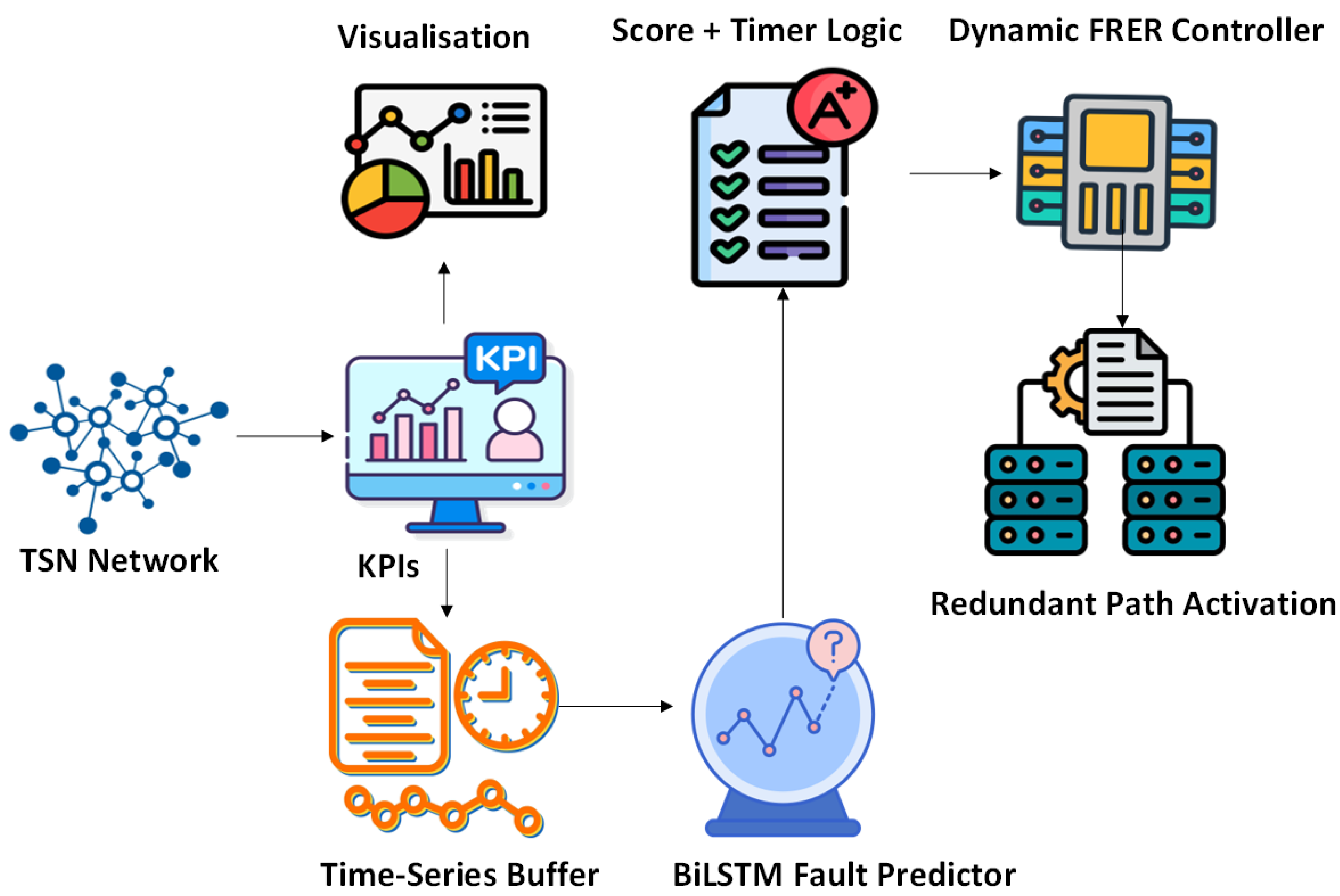
Figure 2.
Sliding window approach is used to construct input sequences for BiLSTM training. Each input sample consists of T consecutive KPI vectors extracted from flow telemetry and is labeled with the class corresponding to the final time step in the sequence. The window advances one step at a time, generating overlapping samples that allow the model to learn predictive patterns from temporal dependencies in the data.
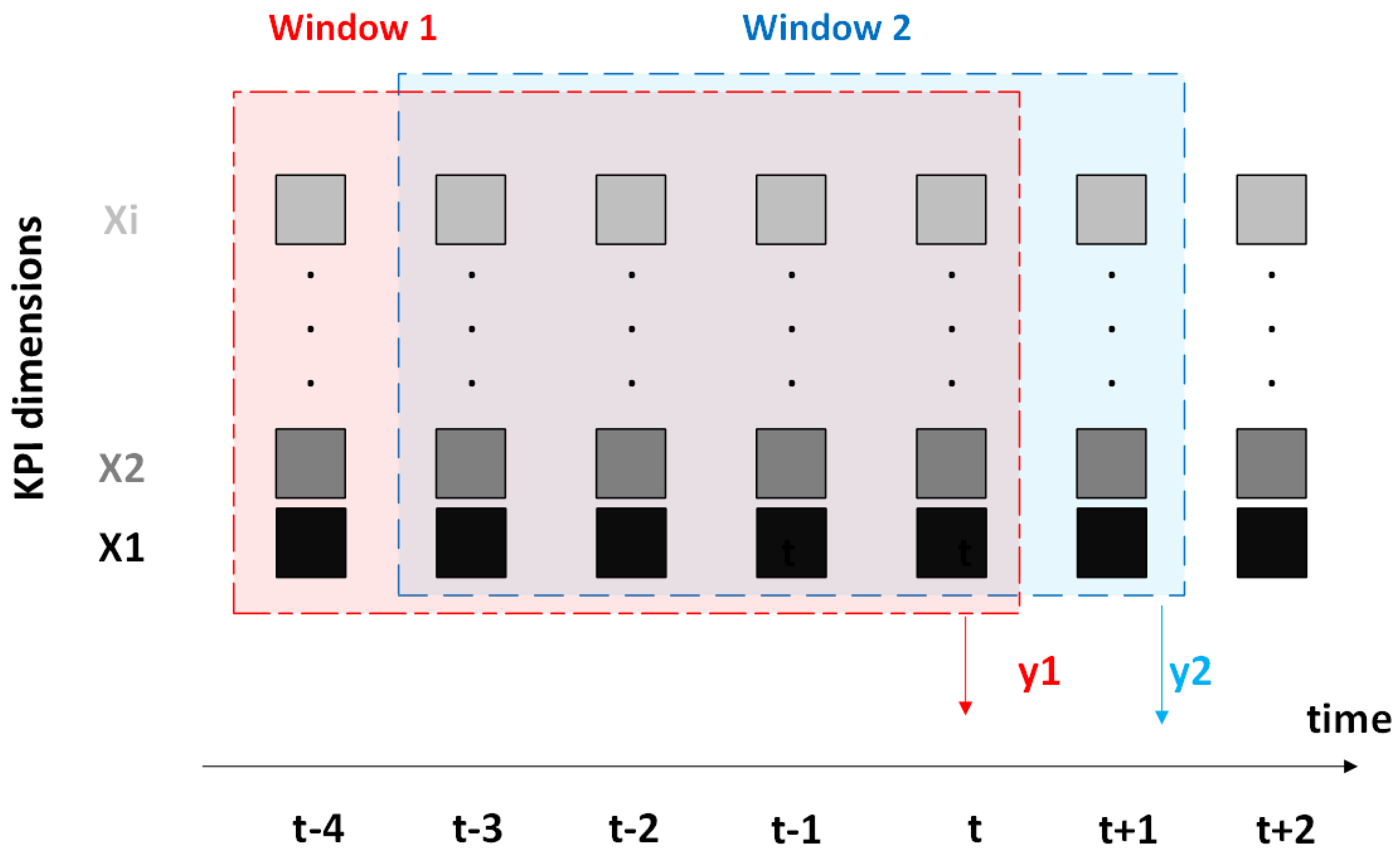
Figure 3.
BiLSTM architecture for time-series fault classification. A sequence of KPI vectors is processed by two stacked bidirectional LSTM layers to extract both forward and backward temporal features. The final hidden states from each direction are concatenated and passed to a fully connected output layer, which produces a softmax distribution over three fault classes: normal, degraded, and recovery.
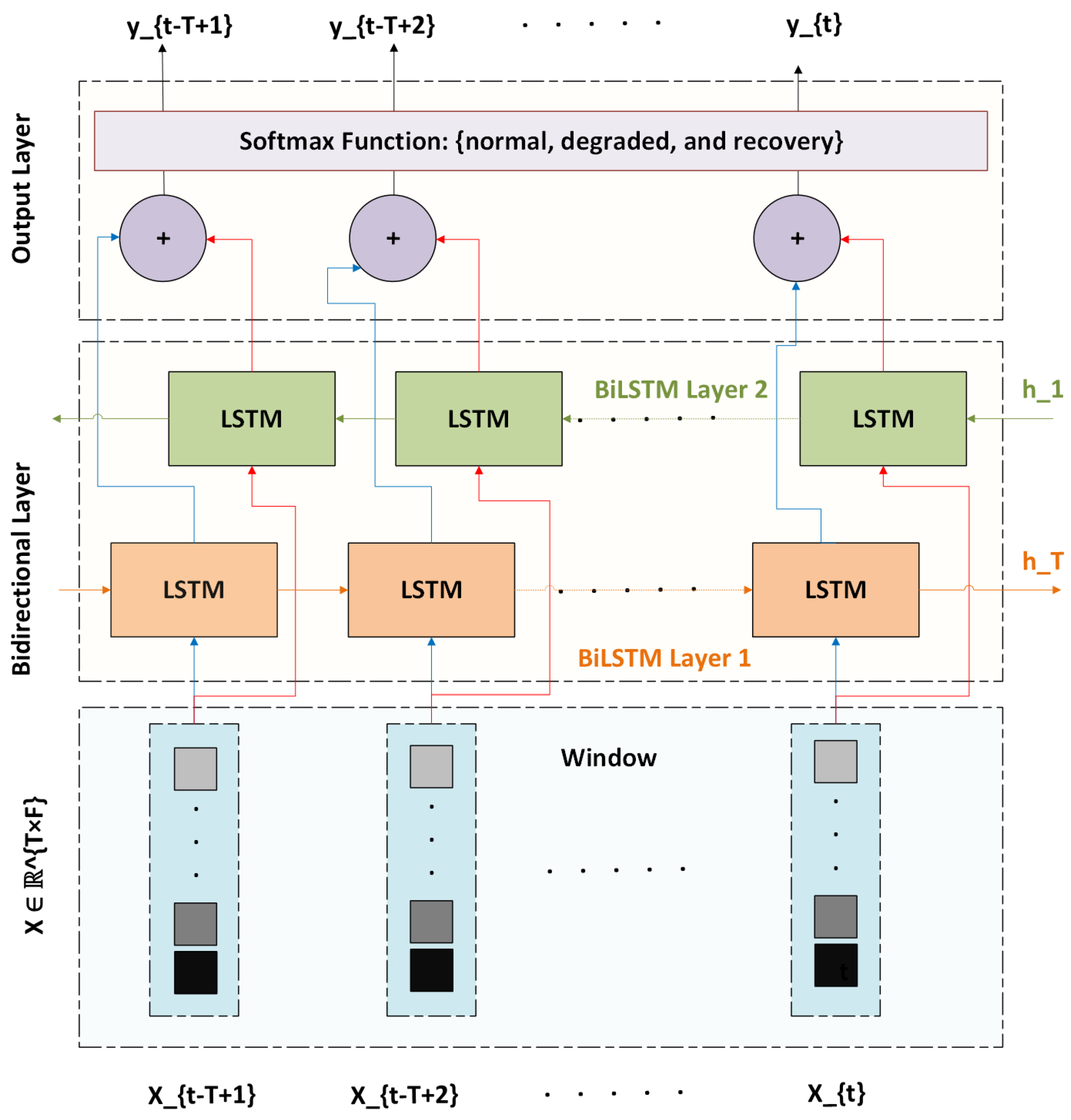
Figure 4.
Finite State Machine (FSM) for FRER control. Transitions are based on model predictions and timers. Circular nodes represent operational states; T1–T5 denote transition triggers.
Figure 4.
Finite State Machine (FSM) for FRER control. Transitions are based on model predictions and timers. Circular nodes represent operational states; T1–T5 denote transition triggers.
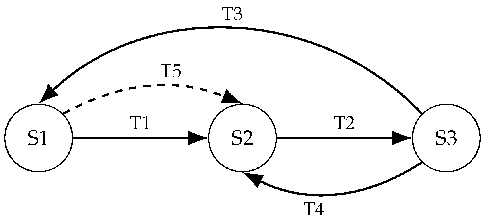
Figure 5.
Visualization of predicted fault states, fault injections, and FRER activation over time, as displayed in the runtime dashboard. Orange markers indicate model predictions of the degraded state, blue markers represent normal predictions, and black crosses denote injected fault events. Shaded red regions correspond to periods during which FRER was active. Notably, FRER activation only occurs after the model outputs a degraded prediction for a consecutive sequence of steps, as defined by the confirmation window. Once activated, FRER remains enabled for at least the duration of the safe window. Deactivation is deferred until both the recovery threshold and timing constraints are satisfied, ensuring stable and fault-resilient behavior.
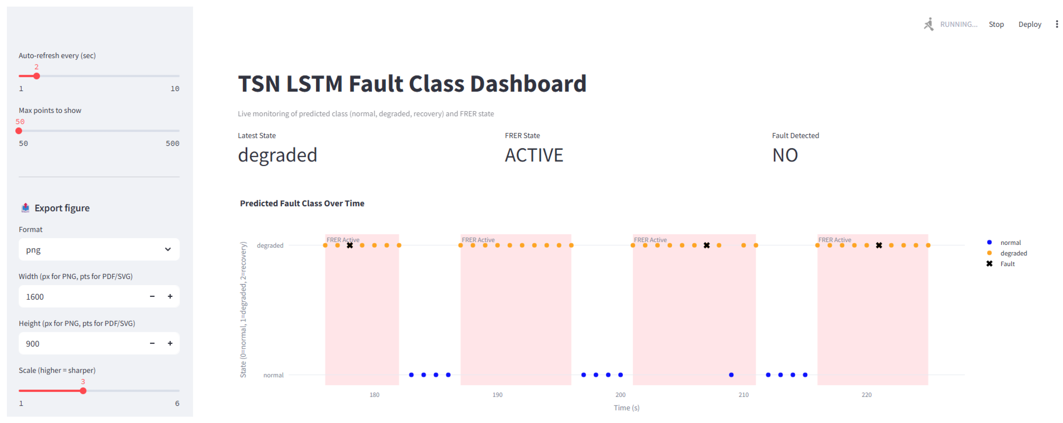
Figure 6.
Runtime trace from the integrated dashboard showing predicted fault classes (colored dots), FRER activation intervals (shaded regions), and injected faults (black × markers). The predictive system consistently activates FRER before or at the onset of degradation, and maintains protection during clustered or recurring faults. Redundancy is automatically withdrawn following sustained recovery.
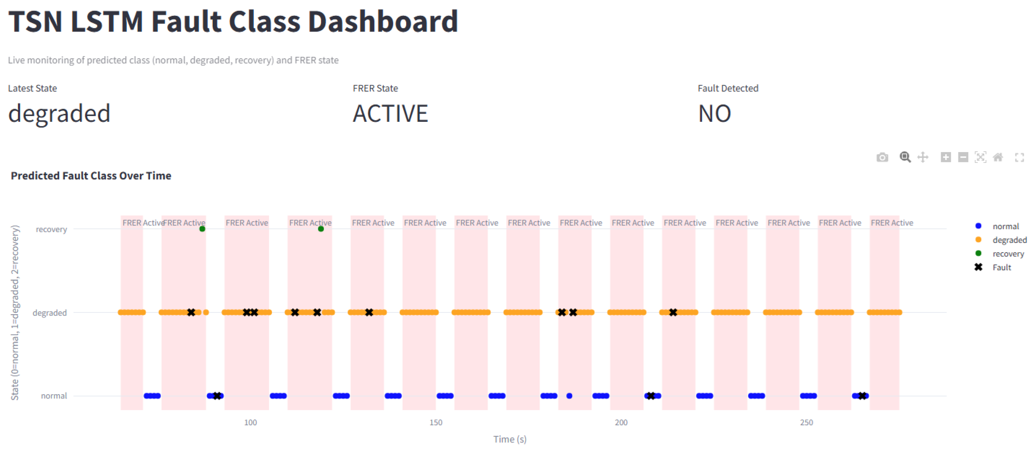
Figure 7.
Comparison of FRER activation time across four fault scenarios. Static FRER remains continuously active, while the predictive system enables redundancy selectively, reducing FRER usage by up to 97.7% in fault-free conditions and by over 60% in fault-prone cases.
Figure 7.
Comparison of FRER activation time across four fault scenarios. Static FRER remains continuously active, while the predictive system enables redundancy selectively, reducing FRER usage by up to 97.7% in fault-free conditions and by over 60% in fault-prone cases.
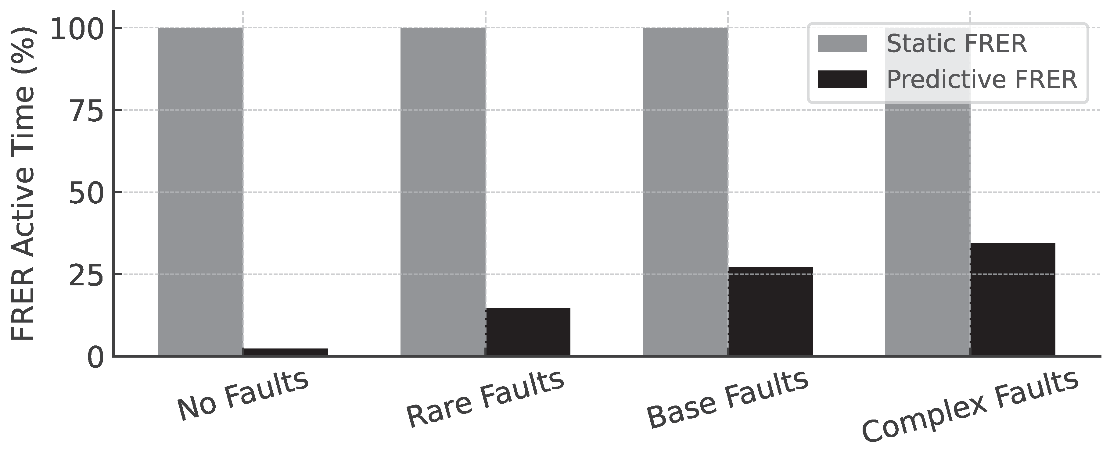
Table 1.
Summary of Evaluation Scenarios.
| Scenario | Fault Rate | Description |
|---|---|---|
| No Faults | 0% | Baseline case with fully stable network conditions. Used to assess false activations and measure unnecessary redundancy under static FRER. |
| Rare Faults | Low | Infrequent and short-lived degradation events. Predictive FRER is expected to remain mostly inactive unless faults persist. |
| Base Faults | Moderate | Regular transient faults representing common industrial conditions such as periodic congestion or wireless interference. Requires active FRER engagement and correct recovery logic. |
| Complex Faults | High/Bursty | Overlapping or closely spaced faults. Designed to test safe window enforcement, reactivation stability, and fault recovery tracking. |
Disclaimer/Publisher’s Note: The statements, opinions and data contained in all publications are solely those of the individual author(s) and contributor(s) and not of MDPI and/or the editor(s). MDPI and/or the editor(s) disclaim responsibility for any injury to people or property resulting from any ideas, methods, instructions or products referred to in the content. |
© 2025 by the authors. Licensee MDPI, Basel, Switzerland. This article is an open access article distributed under the terms and conditions of the Creative Commons Attribution (CC BY) license (http://creativecommons.org/licenses/by/4.0/).
Copyright: This open access article is published under a Creative Commons CC BY 4.0 license, which permit the free download, distribution, and reuse, provided that the author and preprint are cited in any reuse.


