Gamma Regression Model for Insurance Claims Analysis: A Comparative Study on Link Functions and Their Influence on Cost Predictions

1. Introduction

Among these is the Gamma Regression Model. It is a form of Generalized Linear Model (GLM), a framework for estimating dependent variables that have various forms of distribution, particularly when the normal distribution is not appropriate [1,2,3]. The Gamma regression model has been widely used to analyze continuous data when the response variable is positively skewed and is appropriate for data in which variables are strictly positive and tend to be large.

Generalized linear models or GLMs were introduced by Nelder and Wedderburn in 1972 [4] as an extension of the classical linear model in which the response variable is not restricted to being normally distributed. This extension provides flexibility in the statistics being used, making Generalized Linear Model (GLM) statistics more user-friendly than conventional models. GLM enables the testing of all hypotheses that can be tested under GLM, but it has more flexibility in the assumptions that can be made about the distribution of the underlying errors. The main difference is that while the errors in GLM are assumed to be homogenous and normally distributed, GLM has less restrictive assumptions regarding the errors [5,6,7].

The Gamma Regression Model is frequently used in insurance and finance to model costs associated with positively skewed claims or losses, such as environmental claims or costs in insurance [8]. From this model, it can be established the effect of each independent variable, for example, age, vehicle type, etc., on the overall cost of the claims [9].

2. Literature Review

GLM generalizes classical linear models, allowing the outcome to follow a distribution other than the normal, such as logistic, Poisson, or Gamma. This characteristic of GLM renders it applicable in models where data are distributed in various ways and represents a robust means by which to conduct hypothesis testing in a variety of contexts.

The Gamma Regression Model gives a specific definition to the association between the independent variables and the mean of the dependent variable through the link function. The log or the inverse link function is frequently employed. These link functions modify the predicted mean and enable the model to effectively accommodate positively skewed data [10].

The model has a large application scope and is especially common in insurance for claims data analysis. The Gamma distribution is appropriate for modeling strictly positive continuous random variables such as the cost of claims or costs associated with losses from damages [11]. This model gives us insight into how varying each one of these factors, for example, the vehicle’s age or model, impacts the claims cost.

The Gamma distribution’s characteristics and uses are discussed in this paper, which serves to introduce the Gamma distribution in statistical modeling [12].

In addition to introducing generalized linear models with a discussion of link functions (e.g., the Gamma distribution), this book represents an excellent resource on binary and other kinds of dependent variables [13].

Generalized linear models, of which the Gamma regression model is an example, are covered throughout this textbook, as theoretical developments and presentations of GLMs with examples are found throughout [14].

Despite being centered on Bayesian methods, this work contains information on the Gamma distribution, general linear models, and their applications in the real world (among others, insurance and economics), [15].

In this paper, we investigate the application of count data models that are generalized, specifically, generalized linear models that can be used to model over-dispersed count data, thereby providing a broader perspective on the application of GLMs in econometrics [16].

A foundational textbook on the theory and application of generalized linear models, including Gamma regression, with a focus on model fitting, diagnostics, and interpretation of results [17].

A seminal work that introduced the GLM framework, covering various link functions and distributions, including the Gamma distribution, which is integral to this research [18].

This textbook offers extensive coverage of econometric techniques, including generalized linear models for various data types, with applications to the analysis of insurance and economic data [19].

This paper discusses the extension of generalized linear models to include random effects, which may be relevant when modeling more complex data structures, including insurance claims.

This book explores the generalization of logistic regression to other types of data, including the use of the Gamma distribution in regression models, and provides examples of applications in insurance and risk management.

3. Regression Model

Assume that the dependent variable y follows a Gamma distribution with parameters (θ) and$\left(\mu \right)$, where θ represents the shape parameter and $\mu$ is the expected mean of the dependent variable [20]. The regression model is mathematically represented as follows [21,22,23]:

$$f\left(y\right)={\displaystyle \frac{{\lambda }^r}{\mathsf{\Gamma }\left(r\right)}}{y}^{r-1}{e}^{-\lambda y},y>0$$

(1)

The mean $\mu$ is linked to the independent variables$x$ through a link function $g\left(\mu \right)$as:

$$y_i=Exp(x_i^T{\beta }_j+{\epsilon }_i)$$

(2)

In the Gamma Regression Model, common link functions include the logarithmic or inverse link functions, which help connect the independent variables with the dependent variable [24,25,26]. For example, in insurance claim data, the model may use a log link to estimate the average claims cost based on several factors like vehicle age, vehicle type, and number of claims [27,28].

4. Research Methodology

A gamma regression analysis was conducted using SPSS to evaluate data obtained from insurance firms [29]. This approach employed a log link function to explore how factors such as vehicle age, model type, and frequency of claims influence claim costs, which served as the response variable [30,31]. The procedure involved several key steps:

• In SPSS, the gamma distribution was selected, along with a power link function.
• The analysis included the input of both the dependent and independent variables, with the number of claims assigned as the weighting factor.
• Output tables were reviewed to interpret how each independent variable affected claim expenses.
• Model adequacy was assessed through statistical measures, including deviance and Pearson Chi-Square tests.

5. Application

The use of a generalized linear model of the suitability of gamma regression for the analysis of non-negative (positive) data [32]. The data set relates to the cost of compensation for damage to insured vehicles. The average compensation amount follows a gamma distribution (as the dependent variable), where the inverse link function is used to connect the expected value of the dependent variable, y, to a linear combination of independent variables [33].$\left(x_1\right)$ insurance age, $x_2$ vehicle class and $x_3$ vehicle model, i.e., its age). Because we have a different number of claims used to calculate the average claim amounts, you can specify the number of claims as the measurement weight $w$, To build a Kama regression model is as follows [34,35,36,37,38]:

The Pearson chi-square method is selected from the set of parameter estimation using the Scale Parameter Method, which is the method used by McCullagh and Nelder to obtain the same results. The rest of the options remain constant, typical of the product [39,40].

Predicted value of linear predictors and the standard deviation of residential are selected to be stored in the data window, which can help us to check any problem in the fit of the model [41]. Then, clicking on OK, we get the following results:

Table 1. Model Information.

Dependent Variable	Average amount of billing
Probability Distribution	Gamma
Link Function	Power (-1)
Scale Weight Variable	Number of Bills

Table 1. Model Information.

Dependent Variable	Average amount of billing
Probability Distribution	Gamma
Link Function	Power (-1)
Scale Weight Variable	Number of Bills

The model information table shows the name of the dependent variable, the probability distribution is Gamma, the correlation function is the inverse function, and the measurement weight variable is represented by the number of requests [42,43,44].

Table 2. Processing Summary of Cases.

	N	Percent
Included	123	96.1%
Excluded	5	3.9%
Total	128	100.0%

Table 2. Processing Summary of Cases.

	N	Percent
Included	123	96.1%
Excluded	5	3.9%
Total	128	100.0%

The summary Table 2 of the case Operations shows that there are (123) views included in the Model (effective) and (5) missing values, and their total is equal to (128).

The information Table 3 for the categorical variable (consisting of three factors) displays the frequency distribution of each category included in the model, showing both the count and the proportion for each.

Table 3. Categorical Variable Information.

			N	Percent
Factor	Policyholder age	60+	16	13.0%
		50-59	16	13.0%
		40-49	16	13.0%
		35-39	15	12.2%
		30-34	16	13.0%
		25-29	16	13.0%
		21-24	15	12.2%
		17-20	13	10.6%
		Total	123	100.0%
	Vehicle group	D	28	22.2%
		C	31	25.2%
		B	32	26.0%
		A	32	26.0%
		Total	123	100.0%
	Vehicle age	10+	28	22.8%
		8-9	31	25.2%
		4-7	32	26.0%
		0-3	32	26.0%
		Total	123	100.0%

Table 3. Categorical Variable Information.

			N	Percent
Factor	Policyholder age	60+	16	13.0%
		50-59	16	13.0%
		40-49	16	13.0%
		35-39	15	12.2%
		30-34	16	13.0%
		25-29	16	13.0%
		21-24	15	12.2%
		17-20	13	10.6%
		Total	123	100.0%
	Vehicle group	D	28	22.2%
		C	31	25.2%
		B	32	26.0%
		A	32	26.0%
		Total	123	100.0%
	Vehicle age	10+	28	22.8%
		8-9	31	25.2%
		4-7	32	26.0%
		0-3	32	26.0%
		Total	123	100.0%

Table 4. Information on Continuous Variables.

		N	Minimum	Maximun	Mean	Std.Deviation
Dependent Variable	Average amount of billing	123	11	850	231.14	117.048
Scale Weight	Number of bills	123	1	434	72.70	92.598

Table 4. Information on Continuous Variables.

		N	Minimum	Maximun	Mean	Std.Deviation
Dependent Variable	Average amount of billing	123	11	850	231.14	117.048
Scale Weight	Number of bills	123	1	434	72.70	92.598

The continuous variable information table shows that we have only two quantitative variables, the dependent variable representing the average compensation value, and the weight representing the number of requests, and provides descriptive statistic for them.

Table 5, he fit quality table provides two Tests for the null hypothesis that the model fits the data exactly. The deviation and chi-square statistics of Pearson Chi-Square are equal to (124.783 and 131.786), which is less than its Tabular value under the level of (0.05) and degrees of freedom equal to (109), which is equal to (134.085), which indicates the suitability of the data for the estimated model and so on for measuring (Scaled) the two Tests. The smaller the information, the more accurate the model is, and it is compared with other estimated models for other distributions to show preference.

Table 5. Goodness of Fit.

	Value	df	Value|df
Deviance	124.783	109	1.145
Scaled Deviance	103.207	109
Pearson Chi-Square	131.786	109	1.209
Scaled Pearson Chi-Square	109.000	109
Log Likelihood	-622.754
Adjusted Log Likelihood	-623.873
Akaike Information Criterion (AIC)	1273.509
Finite Sample Corrected AIC (AICC)	1277.398
Bayesian Information Criterion (BIC)	1312.879
Consistent AIC(CAIC)	1326.879

Table 5. Goodness of Fit.

	Value	df	Value|df
Deviance	124.783	109	1.145
Scaled Deviance	103.207	109
Pearson Chi-Square	131.786	109	1.209
Scaled Pearson Chi-Square	109.000	109
Log Likelihood	-622.754
Adjusted Log Likelihood	-623.873
Akaike Information Criterion (AIC)	1273.509
Finite Sample Corrected AIC (AICC)	1277.398
Bayesian Information Criterion (BIC)	1312.879
Consistent AIC(CAIC)	1326.879

Table 6. Omnibus Test^a.

Likelihood Ratio Chi-Square	df	Sig.
434.299	13	0.000

Table 6. Omnibus Test^a.

Likelihood Ratio Chi-Square	df	Sig.
434.299	13	0.000

Dependent Variable: Average amount of billing

Mode: (Intercept), Policyholder age, Vehicle group, Vehicle age

• Compares the fitted model against the intercept-only model.

The omnibus test table or weighting ratio tests show the contribution of the influence of variables to the model. (-2 log weighting) is calculated for the reduced model (the model without the influence of these variables, that is, for the constant value only) with the effect of the full model and the value of-p is to test the difference between the two models to indicate the significance of the parameters of the variables as a whole; the value of-p is equal to zero (less than 0.05) the independent variables contribute to the interpretation of the model [46].

Table 7. Tests of Model Effects.

Type III
Source	Wald Chi-Square	df	Sig.
(Intercept)	1440.320	1	0.000
Policyholder age	57.613	7	0.000
Vehicle group	136.430	3	0.000
Vehicle age	136.016	3	0.000

Table 7. Tests of Model Effects.

Type III
Source	Wald Chi-Square	df	Sig.
(Intercept)	1440.320	1	0.000
Policyholder age	57.613	7	0.000
Vehicle group	136.430	3	0.000
Vehicle age	136.016	3	0.000

Dependent Variable: Average amount of billing

Model: (Intercept), Policyholder age, Vehicle group, Vehicle age

Table 7 of the model effects tests shows the significance of all the parameters of the independent variables in the model because all the values of p are equal to zero and are less than the significance level (0.05), as observed by the statistic of the father (Kai quadrature), which were all greater than their Tabular values [47,48].

Comprehensive testing and model effects tests (not shown) indicate that the overall model is superior to the empty model and that each of the main effects contributes to the model. The table of parameter estimates shows the same values obtained by Makula and Nelder for the factor levels and the scale parameter [49,50]. Look at the estimated marginal or marginal circles to explain the relationships between factor levels.

The parameter estimation table summarizes the effect of each factor at each level (category). Squaring the ratio of the coefficient to its standard error is equal to Wald’s statistic. If the values of p for the parent statistic are small (less than 0.05), then the parameter differs from zero, and there is a significant influence of that factor at that level.

Table 8. Parameter Estimates.

			95% Wald Confidence Interval		Hypothesis Test
Parameter	B	Std. Error	Lower	Upper	Wald Chi-Square	df	Sig
(Intercept)	0.003	0.0004	0.003	0.004	66.593	1	0.000
[Policyholder age=8]	0.001	0.0004	0.000	0.002	4.898	1	0.027
[Policyholder age=7]	0.001	0.0004	0.000	0.002	5.046	1	0.025
[Policyholder age=6]	0.001	0.0004	0.000	0.002	5.740	1	0.017
[Policyholder age=5]	0.001	0.0004	0.001	0.002	10.682	1	0.001
[Policyholder age=4]	0.000	0.0004	0.000	0.001	1.268	1	0.260
[Policyholder age=3]	0.000	0.0004	0.000	0.001	0.720	1	0.396
[Policyholder age=2]	0.000	0.0004	-0.001	0.001	0.054	1	0.816
[Policyholder age=1]	0a						.
[Vehicle group=4]	-0.001	0.0002	-0.002	0.001	61.883	1	0.000
[Vehicle group=3]	-0.001	0.0002	-0.001	0.000	13.039	1	0.000
[Vehicle group=2]	3.765E-5	0.0002	0.000	0.000	0.050	1	0.823
[Vehicle group=1]	0a						.
[Vehicle age=4]	0.004	0.0004	0.003	0.005	88.175	1	0.000
[Vehicle age=13	0.002	0.0002	0.001	0.002	53.013	1	0.000
[Vehicle age=2]	0.000	0.0001	0.000	0.001	13.191	1	0.000
[Vehicle age=1]	0a						.
Scale	1.209b

Table 8. Parameter Estimates.

			95% Wald Confidence Interval		Hypothesis Test
Parameter	B	Std. Error	Lower	Upper	Wald Chi-Square	df	Sig
(Intercept)	0.003	0.0004	0.003	0.004	66.593	1	0.000
[Policyholder age=8]	0.001	0.0004	0.000	0.002	4.898	1	0.027
[Policyholder age=7]	0.001	0.0004	0.000	0.002	5.046	1	0.025
[Policyholder age=6]	0.001	0.0004	0.000	0.002	5.740	1	0.017
[Policyholder age=5]	0.001	0.0004	0.001	0.002	10.682	1	0.001
[Policyholder age=4]	0.000	0.0004	0.000	0.001	1.268	1	0.260
[Policyholder age=3]	0.000	0.0004	0.000	0.001	0.720	1	0.396
[Policyholder age=2]	0.000	0.0004	-0.001	0.001	0.054	1	0.816
[Policyholder age=1]	0a						.
[Vehicle group=4]	-0.001	0.0002	-0.002	0.001	61.883	1	0.000
[Vehicle group=3]	-0.001	0.0002	-0.001	0.000	13.039	1	0.000
[Vehicle group=2]	3.765E-5	0.0002	0.000	0.000	0.050	1	0.823
[Vehicle group=1]	0a						.
[Vehicle age=4]	0.004	0.0004	0.003	0.005	88.175	1	0.000
[Vehicle age=13	0.002	0.0002	0.001	0.002	53.013	1	0.000
[Vehicle age=2]	0.000	0.0001	0.000	0.001	13.191	1	0.000
[Vehicle age=1]	0a						.
Scale	1.209b

Dependent Variable: Average amount of billing.

Model: (Intercept), Policyholder age, Vehicle group, Vehicle age.

• Set to zero because this parameter is redundant.
• Computed based on the Pearson chi-square.

Table 9. Estimated Marginal Means 1: Policyholder age.

		Estimates
			95% Wald Confidence Interval
Policyholder age	Mean	Std. Error	Lower	Upper
60+	186.08	6.084	174.87	198.82
50-59	186.20	5.551	175.92	197.75
40-49	184.38	5.155	174.80	195.07
35-39	171.70	5.516	161.53	183.24
30-34	203.40	6.930	190.67	217.95
25-29	208.15	7.482	194.46	223.93
21-24	219.52	10.824	200.17	243.00
17-20	224.51	20.690	190.16	274.00

Table 9. Estimated Marginal Means 1: Policyholder age.

		Estimates
			95% Wald Confidence Interval
Policyholder age	Mean	Std. Error	Lower	Upper
60+	186.08	6.084	174.87	198.82
50-59	186.20	5.551	175.92	197.75
40-49	184.38	5.155	174.80	195.07
35-39	171.70	5.516	161.53	183.24
30-34	203.40	6.930	190.67	217.95
25-29	208.15	7.482	194.46	223.93
21-24	219.52	10.824	200.17	243.00
17-20	224.51	20.690	190.16	274.00

The insurance age table presents the model-derived marginal means, along with their corresponding standard errors and confidence intervals, for the average claim cost — which serves as the dependent variable. This information helps in examining how the average claim cost varies across different age categories. In the given case, these marginal means span from 171.70 in the 35–39 age group to 224.51 in the 17–20 age group. To determine whether these observed differences are statistically meaningful or merely the result of random variation, one should refer to the associated test statistics [51,52].

Table 10. Individual Test Results.

Policyholder age Repeated Contrast	Contrast Estimate	Std. Error	Wald Chi-Square	df	Sequential Sidak Sig.
Level 60+vs. Level 50-59	-0.13	6.093	0.000	1	0.984
Level 50-59 vs. Level 40-49	1.82	5.068	0.129	1	0.978
Level 35-39 vs. Level 35-39	12.68	5.458	5.397	1	0.115
Level 30-34 vs. Level 30-34	-31.70	6.705	22.351	1	0.000
Level 25-29 vs. Level 25-29	-4.75	7.359	0.417	1	0.946
Level 21-24 vs. Level 21-24	-11.36	10.709	1.125	1	0.818
Level 17-20 vs. Level 17-20	-5.00	21.812	0.052	1	0.978

Table 10. Individual Test Results.

Policyholder age Repeated Contrast	Contrast Estimate	Std. Error	Wald Chi-Square	df	Sequential Sidak Sig.
Level 60+vs. Level 50-59	-0.13	6.093	0.000	1	0.984
Level 50-59 vs. Level 40-49	1.82	5.068	0.129	1	0.978
Level 35-39 vs. Level 35-39	12.68	5.458	5.397	1	0.115
Level 30-34 vs. Level 30-34	-31.70	6.705	22.351	1	0.000
Level 25-29 vs. Level 25-29	-4.75	7.359	0.417	1	0.946
Level 21-24 vs. Level 21-24	-11.36	10.709	1.125	1	0.818
Level 17-20 vs. Level 17-20	-5.00	21.812	0.052	1	0.978

Table 10 of individual test results compares consecutive insurance age groups and determines whether the differences observed are statistically significant or due to chance. Only one significant difference was found between the 30-34 and 35-39 age groups (p-value = 0.000). This suggests that these two groups are distinct, with younger insurance policies showing higher compensation costs. There is also some indication, though not statistically significant, that the number of claims first decreases and then increases as the insurance age progresses.

Table 11. Summary of Test Results.

Wald Chi-Square	df	Sig.
47.925	7	0.000

Table 11. Summary of Test Results.

Wald Chi-Square	df	Sig.
47.925	7	0.000

The Comprehensive Test table presents the results for all comparisons listed in the individual test results table. A p-value of zero indicates a significant difference in insurance compensation costs across the different categories or levels of insurance age. It is important to note that this test is not the same as the model effects test for insurance duration, as the latter is conducted on a transformed scale, whereas the estimated marginal means are calculated on the original scale.

Table 12. Estimates.

			95% Wald Confidence Interval
Vehicle group	Mean	Std.Error	Lower	Upper
D	239.87	9.513	222.57	260.08
C	200.98	6.168	189.58	213.84
B	177.71	4.668	169.02	187.34
A	178.91	5.871	168.09	191.20

Table 12. Estimates.

			95% Wald Confidence Interval
Vehicle group	Mean	Std.Error	Lower	Upper
D	239.87	9.513	222.57	260.08
C	200.98	6.168	189.58	213.84
B	177.71	4.668	169.02	187.34
A	178.91	5.871	168.09	191.20

Table 12 shows the estimated marginal averages for the vehicle class (type or model), standard errors, and confidence intervals of the average cost of insurance compensation at the levels of the vehicle type factor. This table is useful for exploring the differences between the levels of this factor. In this example, the marginal averages range from 177.71 for the Type B vehicle to the highest 239.87 for the Type D vehicle. To find out if the values in this table represent real differences or are likely due to chance, look at the test results.

Table 13. Pairwise Comparisons.

						95% Wald Confidence Interval Differencea
(I)Vehicle group	(J)Vehicle group	Mean Difference (I-J)	Std. Error	df	Sequential Sidak Sig.	Lower	Upper
D	C	38.89a	6.953	1	0.000	21.57	56.21
	B	62.16a	7.338	1	0.000	42.85	81.47
	A	60.96a	8.527	1	0.000	39.06	82.87
C	D	-38.89a	6.953	1	0.000	-56.21	-21.57
	B	23.27a	4.406	1	0.000	12.75	33.79
	A	22.07a	6.020	1	0.000	8.61	35.54
B	D	-62.16a	7.338	1	0.000	-81.47	-42.85
	C	-23.27a	4.406	1	0.000	-33.79	-12.75
	A	-1.20	5.378	1	0.824	-11.74	9.34
A	D	-60.96a	8.527	1	0.000	-82.87	-39.06
	C	-22.07a	6.020	1	0.000	-35.54	-8.61
	B	1.20	5.378	1	0.824	-9.34	11.74

Table 13. Pairwise Comparisons.

						95% Wald Confidence Interval Differencea
(I)Vehicle group	(J)Vehicle group	Mean Difference (I-J)	Std. Error	df	Sequential Sidak Sig.	Lower	Upper
D	C	38.89a	6.953	1	0.000	21.57	56.21
	B	62.16a	7.338	1	0.000	42.85	81.47
	A	60.96a	8.527	1	0.000	39.06	82.87
C	D	-38.89a	6.953	1	0.000	-56.21	-21.57
	B	23.27a	4.406	1	0.000	12.75	33.79
	A	22.07a	6.020	1	0.000	8.61	35.54
B	D	-62.16a	7.338	1	0.000	-81.47	-42.85
	C	-23.27a	4.406	1	0.000	-33.79	-12.75
	A	-1.20	5.378	1	0.824	-11.74	9.34
A	D	-60.96a	8.527	1	0.000	-82.87	-39.06
	C	-22.07a	6.020	1	0.000	-35.54	-8.61
	B	1.20	5.378	1	0.824	-9.34	11.74

Pairwise comparisons of estimated marginal means based on the original scale of the dependent variable, Average amount of billing:

• The mean difference is significant at the 0.05 level.
• Confidence interval bounds are approximate.

The pairwise comparison table shows the differences between each pair of vehicle types and tests whether each difference is due to a coincidence difference. Comparison of only types of compounds A and B is not statistically significant (the value of p is equal to 0.824). These two groups are associated with the lowest claims (the cost of insurance compensation), followed by Type C, and then Type D, with the highest number of claims.

Table 14. Overall Test Results.

Wald Chi-Square	df	Sig.
78.468	3	0.000

Table 14. Overall Test Results.

Wald Chi-Square	df	Sig.
78.468	3	0.000

The Wald chi-square tests the effect of the Vehicle group. This test is based on the linearly independent pairwise comparisons among the estimated marginal means

The table shows the results of the Comprehensive Test of all antagonists in the pairwise comparisons table, and a value of p equal to zero indicates a significant difference between the cost of insurance compensation depending on the categories or levels of the vehicle class. This test is not equivalent to the model effects test for the vehicle class because the model effects test is performed on the converted scale, while these estimated limit averages were calculated on the original scale.

Table 15. Estimates.

			95% Wald Confidence Interval
Vehicle age	Mean	Std. Error	Lower	Upper
10+	129.85	7.404	116.80	146.19
8-9	192.35	8.227	177.48	209.95
4-7	255.50	5.976	244.30	267.78
0-3	281.89	6.620	269.48	295.49

Table 15. Estimates.

			95% Wald Confidence Interval
Vehicle age	Mean	Std. Error	Lower	Upper
10+	129.85	7.404	116.80	146.19
8-9	192.35	8.227	177.48	209.95
4-7	255.50	5.976	244.30	267.78
0-3	281.89	6.620	269.48	295.49

This table displays the model-estimated marginal means, along with the associated standard errors and confidence intervals, for the average cost of insurance compensation across different levels of the vehicle age factor. It serves as a useful tool for examining variations among these levels. In this case, the independent variable ranges from a low of 129.85 for vehicles older than 10 years to a high of 281.89 for vehicles aged between 0 and 3 years. To assess whether these observed differences are statistically significant or potentially due to random variation, one should consult the corresponding test results.

Table 16. Individual Test Results.

Vehicle age Repeated Contrast	Contrast Estimate	Std. Error	Wald Chi-Square	df	Sequential Sidak Sig.
Level 10+vs. Level 8-9	-62.50	10.889	32.947	1	0.000
Level 8-9 vs. Level 4-7	-63.15	9.544	43.783	1	0.000
Level 4-7 vs. Level 0-3	-26.38	7.268	13.175	1	0.000

Table 16. Individual Test Results.

Vehicle age Repeated Contrast	Contrast Estimate	Std. Error	Wald Chi-Square	df	Sequential Sidak Sig.
Level 10+vs. Level 8-9	-62.50	10.889	32.947	1	0.000
Level 8-9 vs. Level 4-7	-63.15	9.544	43.783	1	0.000
Level 4-7 vs. Level 0-3	-26.38	7.268	13.175	1	0.000

Table 16 of the results of individual tests shows the differences between the successive age groups of the vehicle and tests whether each difference is due to chance. All antagonists are statistically significant because all values of p are equal to zero, which is strong evidence that the volume of claims (the cost of insurance compensation) decreases as the vehicle ages.

Table 17. Overall Test Results.

Wald Chi-Square	df	Sig.
282.315	3	0.000

Table 17. Overall Test Results.

Wald Chi-Square	df	Sig.
282.315	3	0.000

The Comprehensive Test table shows the test results for all antagonists in the pairwise comparisons table, and a p-value equal to zero indicates a significant difference between the cost of insurance compensation depending on the categories or age levels of vehicles. This test is not equivalent to the model effects test for the age of the vehicle because the model effects test is performed on the converted scale, while these estimated limit averages were calculated on the original scale.

To verify the formulation of the model, look at the drawing of the standard deviation residuals against the estimated linear independent variables. The spread plot of the standard deviation residuals against the expected values of the linear forecast was performed as follows:

Figure 1. Simple Scatter Standardized Residual.

Figure 1. Simple Scatter Standardized Residual.

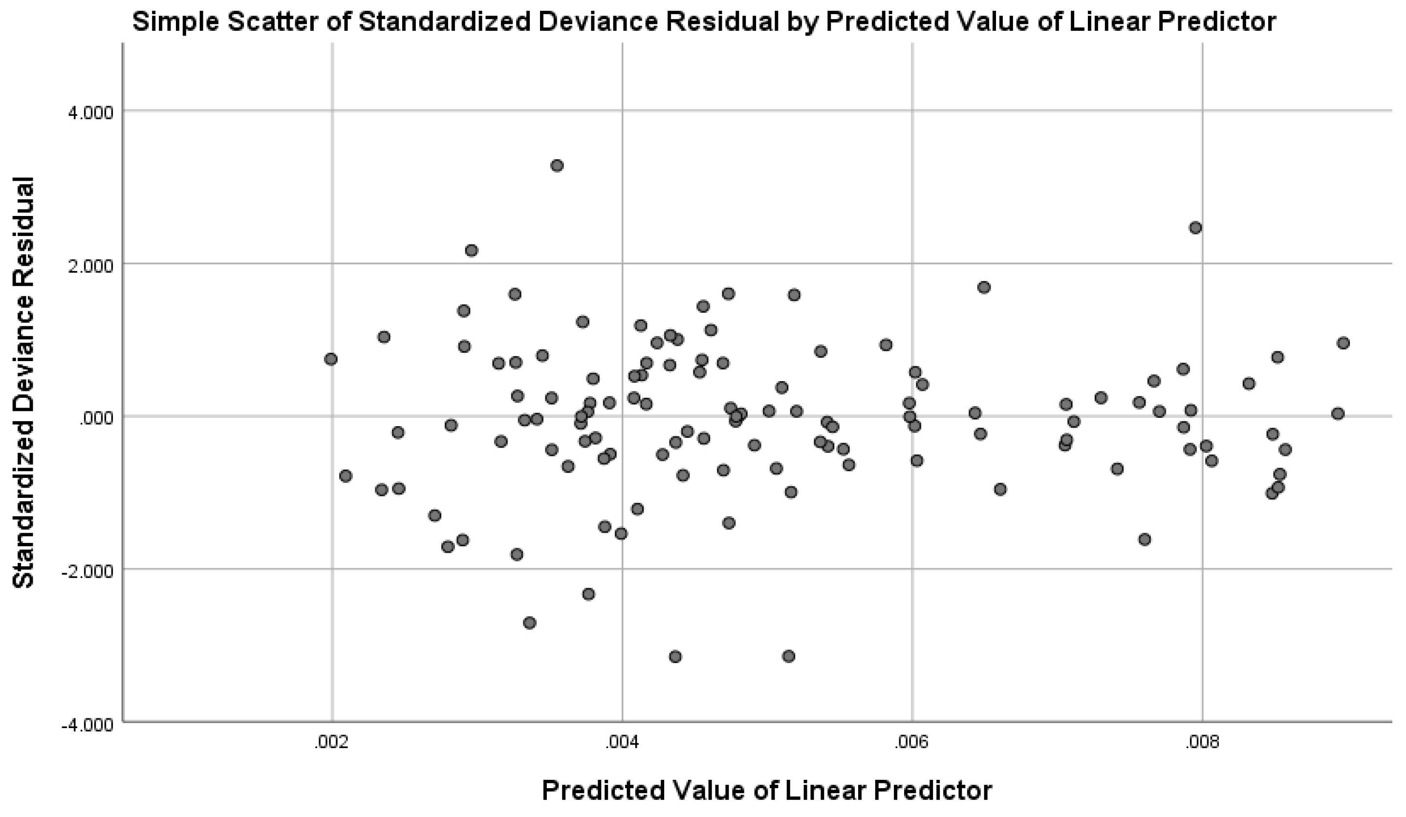
Some points are outside the General Group and can be investigated further, but otherwise, there is nothing suspicious in the drawing.

6. Results

After fitting the model, detailed results were obtained, including parameter estimates and hypothesis testing. The results indicated that the independent variables, such as vehicle age and vehicle type, have a significant impact on the cost of claims. The p-values for all independent variables were less than 0.05, indicating that there is a statistically significant relationship between these factors and the dependent variable.

Comparison of Link Functions:

The results were compared using logarithmic link and inverse link functions. It was found that the logarithmic link function provided a better fit, as it resulted in lower deviance statistics and Pearson Chi-Square values compared to the inverse link function.

7. Conclusions

The Gamma Regression Model is a powerful tool for analyzing data that follows a Gamma distribution. The use of the logarithmic link function proved to be more effective in modeling the cost of insurance claims compared to the inverse link function. By applying this model, insurance companies can better understand the factors influencing claims costs, leading to more informed decisions and improved risk management strategies.

The Gamma Regression Model offers a robust and flexible framework for modeling positive continuous data, particularly when the data exhibit a skewed distribution. This model, part of the Generalized Linear Models (GLM) family, is especially useful in cases where traditional assumptions of normality do not hold, such as in the analysis of insurance claims, environmental damage costs, or other economic applications.

In this study, the application of the Gamma Regression Model using SPSS has demonstrated its effectiveness in analyzing the cost of insurance claims. By applying various link functions, specifically the logarithmic link function, the study found that it provides the best fit compared to the inverse link function, as evidenced by lower deviance statistics and Pearson Chi-Square values. This highlights the importance of selecting the appropriate link function for better model accuracy.

The results from this study also emphasize the significance of independent variables such as vehicle age and vehicle type in determining the cost of claims. The statistical significance of these variables provides valuable insights into the factors that drive insurance costs, allowing insurance companies to make more informed decisions in terms of risk management and pricing strategies.

Overall, the Gamma Regression Model proves to be an essential tool in analyzing non-negative, skewed data, and its flexibility in handling various types of data distributions makes it a highly valuable technique in multiple fields, including finance, insurance, and environmental economics.

References

- Ali, T. H. (2022). Modification of the adaptive Nadaraya-Watson kernel method for nonparametric regression (simulation study). Commun. Stat.—Simul. Comput., 51(2), 391–403. [CrossRef]
- Mustafa, Qais, and Ali, Taha Hussein. “Comparing the Box Jenkins models before and after the wavelet filtering in terms of reducing the orders with application.” Journal of Concrete and Applicable Mathematics 11 (2013): 190-198.
- Ali, Taha Hussein, Heyam Abd Al-Majeed Hayawi, and Delshad Shaker Ismael Botani. “Estimation of the bandwidth parameter in Nadaraya-Watson kernel non-parametric regression based on universal threshold level.” Communications in Statistics-Simulation and Computation 52.4 (2023): 1476-1489. [CrossRef]
- Nelder, J.A., & Wedderburn, R.W.M. (1972). Generalized linear models. Journal of the Royal Statistical Society, Series A (General), 135(3), 370-384.
- Heyam A. Hayawi, (2022) Using wavelet in identification state space models. Int. J. Nonlinear Ann. Appl. 1 (13), 2573-2578.
- Ahmed K. Husein, Heyam A. Hayawi,(2022),”Diagnostic and Prediction For the Models of state spaces and transfer function model-A Contrastive Study”, AL-Anbar University journal of Economic and Administration Sciences,11(25),514-530.
- Heyam A. Hayawi, Najlaa Saad Ibrahim Alsharabi,(2022),”Analysis of multivariate time series for some linear models by using multi-dimensional wavelet shrinkage”,Periodicals of Engineering and Natural Sciences 10 (4), 120-129.
- Ali, Taha Hussein, and Jwana Rostam Qadir. “Using Wavelet Shrinkage in the Cox Proportional Hazards Regression model (simulation study)”, Iraqi Journal of Statistical Sciences, 19, 1, 2022, 17-29. https://stats.uomosul.edu.iq/article_174328.html. [CrossRef]
- Ali, Taha Hussein, and Dlshad Mahmood Saleh. “COMPARISON BETWEEN WAVELET BAYESIAN AND BAYESIAN ESTIMATORS TO REMEDY CONTAMINATION IN LINEAR REGRESSION MODEL” PalArch’s Journal of Archaeology of Egypt/Egyptology 18.10 (2021): 3388-3409. https://www.archives.palarch.nl/index.php/jae/ article/view/10382/9524.
- Heyam A. Hayawi, Ibrahim, Najlaa Saad, (2022),” Comparison of prediction using Matching Pattern and state space models”, IRAQI JOURNAL OF STATISTICAL SCIENCES 19 (1), 30-37. [CrossRef]
- Ali, Taha Hussien, (2017), “Using Proposed Nonparametric Regression Models for Clustered Data (A simulation study).” ZANCO Journal of Pure and Applied Sciences, 29.2: 78-87. https://www.researchgate.net/publication/343626707_Using_Proposed_Nonparametric_Regression_Models_for_Clustered_Data_A_simulation_studypdf.
- McCullagh, P., & Nelder, J.A. (1989). Generalized Linear Models. Chapman and Hall.
- Dobson, A.J. (2002). An Introduction to Generalized Linear Models. Chapman and Hall.
- Aitchison, J., & Ho, C. (1989). The Gamma Distribution: A Review and Some Applications. Journal of the Royal Statistical Society, Series B (Methodological), 51(3), 336-355.
- Cox, D.R., & Snell, E.J. (1989). Analysis of Binary Data. Chapman & Hall.
- Hardin, J.W., & Hilbe, J.M. (2007). Generalized Linear Models and Extensions. Stata Press.
- Jackman, S. (2009). Bayesian Analysis for the Social Sciences. Wiley.
- Papke, L.E., & Wooldridge, J.M. (1996). Econometric Methods for Count Data Analysis. Journal of Applied Econometrics, 11(6), 573-604.
- Agresti, A. (2015). Foundations of Linear and Generalized Linear Models. Wiley.
- Nelder, J.A., & McCullagh, P. (1989). Generalized Linear Models. Chapman & Hall.
- Greene, W.H. (2012). Econometric Analysis. Pearson Education.
- Breslow, N.E., & Clayton, D.G. (1993). Approximate Inference in Generalized Linear Models with Random Effects. Journal of the American Statistical Association, 88(421), 9-25.
- Collett, D. (2003). Modelling Binary Data. CRC Press.
- Ali, Taha Hussein, Saman Hussein Mahmood, and Awat Sirdar Wahdi. “Using Proposed Hybrid method for neural networks and wavelet to estimate time series model.” Tikrit Journal of Administration and Economics Sciences 18.57 part 3 (2022). https://www.tjaes.org/index.php/tjaes/article/view/324.
- Thafer Ramathan Muttar ,Heyam A. Hayawi, (2011), ”The Recursive Identification of Stochastic Linear Dynamical Systems Simulation Study”,Iraqi Journal of Statistical Sciences 11 (1),21-54. [CrossRef]
- Ahmed S.Altaee, Heyam A. Hayawi,(2012), ”Employment of the Factor Analysis Approach to Predict the Transfer Function Models”,Iraqi Journal Of Statistical Sciences 12 (1),97-118. [CrossRef]
- Shereen Turky, Heyam A. Hayawi, (2012), ”Prediction Comparison by using Transfer Function Models”, Iraqi Journal of Statistical Sciences 22, 98-120. [CrossRef]
- Ali, Taha Hussien, and Mohammad, Awaz Shahab (2021), Data de-noise for Discriminant Analysis by using Multivariate Wavelets (Simulation with practical application), Journal of Arab Statisticians Union (JASU), 5.3: 78-87. https://search.emarefa.net/detail/BIM-1555851.
- Omar, C., Ali, T. H., & Hassn, K. (2020). Using Bayes weights to remedy the heterogeneity problem of random error variance in linear models. Iraqi Journal of Statistical Sciences, 17(2), 58–67. https://stats.uomosul.edu.iq/article_167391_002eac088c04564fa24970cc53dc749d.pdf. [CrossRef]
- Qais Mustafa Abd alqader and Taha Hussien Ali, (2020), Monthly Forecasting of Water Consumption in Erbil City Using a Proposed Method, Al-Atroha journal, 5.3:47-67. https://www.researchgate.net/publication/353033062_Monthly_Forecasting_of_Water_Consumption_in_Erbil_City_Using_a_Proposed_Method.
- Ali, Taha Hussein, Avan Al-Saffar, and Sarbast Saeed Ismael. “Using Bayes weights to estimate parameters of a Gamma Regression model.” Iraqi Journal of Statistical Sciences 20.1 (2023): 43-54. https://stats.uomosul.edu.iq/article_178687.html. [CrossRef]
- Raza, Mahdi Saber, Taha Hussein Ali, and Tara Ahmed Hassan. “Using Mixed Distribution for Gamma and Exponential to Estimate of Survival Function (Brain Stroke).” Polytechnic Journal 8.1 (2018). [CrossRef]
- Kareem, Nazeera Sedeek, and Taha Hussein Ali. “Awaz Shahab M, (2020),” De-noise data by using Multivariate Wavelets in the Path analysis with application”, Kirkuk University Journal of Administrative and Economic Sciences 10.1: 268-294. https://iasj.rdd.edu.iq/journals/uploads/2024/12/07/f733e78c937d1be5a7bd0cfabd6c1a7e.pdf.
- Ali, Taha Hussein, “Estimation of Multiple Logistic Model by Using Empirical Bayes Weights and Comparing it with the Classical Method with Application” Iraqi Journal of Statistical Sciences 20 (2011): 348-331.
- Ali, Taha Hussein & Mardin Samir Ali. “Analysis of Some Linear Dynamic Systems with Bivariate Wavelets” Iraqi Journal of Statistical Sciences 16.3 (2019): 85-109. https://stats.uomosul.edu.iq/article_164176.html.
- Samad Sedeeq, B., Muhammad, Z. A., Ali, I. M., & Ali, T. H. (2024). Construction Robust -Chart and Compare it with Hotelling’s T2-Chart. Zanco Journal of Human Sciences, 28(1), 140–157. [CrossRef]
- Ali, Taha Hussein; Saleh, Dlshad Mahmood; Rahim, Alan Ghafur. “Comparison between the median and average charts using applied data representing pressing power of ceramic tiles and power of pipe concrete”, Journal of Humanity Sciences 21.3 (2017): 141-149.
- Ali, Taha Hussein; Tara Ahmed Hassan. “Estimating of Logistic Model by using Sequential Bayes Weights”, Journal of Economics and Administrative Sciences, 13.46 (2007): 217-235. [CrossRef]
- Heyam A. Hayawi, Edrees Mohamad Nori, (2009), ”Using maximum distances from unit line to the Embedding vectors to estimate the delay time with an application”, Iraqi Journal of Statistical Sciences 9 (1), 43-62. [CrossRef]
- Heyam A. Hayawi, (2010),” Estimation of State Space Models by using Ridge Regression Technique with Application”, Iraqi Journal of Statistical Sciences 10 (2), 155-176.
- Ali, Taha Hussein; Shaymaa Mohammed Shakir. “Using Bayesian Weighted Method to Estimate the Parameters of Qualitative Regression Depending on Poisson distribution “A comparative Study”, ZANCO Journal of Pure and Applied Sciences, 28.5 (2016): 41-52. [CrossRef]
- Ali, T. H., Sedeeq, B. S., Saleh, D. M., & Rahim, A. G. (2024). Robust multivariate quality control charts for enhanced variability monitoring. Quality and Reliability Engineering International, 40(3), 1369-1381. [CrossRef]
- Haydier, Esraa Awni, Nasradeen Haj Salih Albarwari, and Ali, Taha Hussein. “The Comparison Between VAR and ARIMAX Time Series Models in Forecasting.” Iraqi Journal of Statistical Sciences 20.2 (2023): 249- 262. https://stats.uomosul.edu.iq/article_181260_ff0164e286f9 9f8046e2ee21368235b4.pdf.
- Ali, Taha Hussein, Haider, Israa Awni, and Rasoul, Fatima Othman Hama. “Create a Bayesian panel for the number of weighted defects and compare it with the Shewart panel”. Journal of Business Economics for Applied Research, 5.5 (2023): 305-320. https://iasj.rdd.edu.iq/journals/uploads/2024/12/07/a2d11f761ef87ac4b48e1eb942d6049a.pdf.
- Omer, A. W., Sedeeq, B. S., & Ali, T. H. (2024). A proposed hybrid method for Multivariate Linear Regression Model and Multivariate Wavelets (Simulation study). Polytechnic Journal of Humanities and Social Sciences, 5(1), 112-124. https://journals.epu.edu.iq/index.php /Mitanni/article/view/1452.
- Sakar Ali Jalal; Dlshad Mahmood Saleh; Bekhal Samad Sedeeq; Taha Hussein Ali. “Construction of the Daubechies Wavelet Chart for Quality Control of the Single Value”. IRAQI JOURNAL OF STATISTICAL SCIENCES, 21, 1, 2024, 160-169. [CrossRef]
- Ali, T. H., Raza, M. S., & Abdulqader, Q. M. (2024). VAR TIME SERIES ANALYSIS USING WAVELET SHRINKAGE WITH APPLICATION. Science Journal of University of Zakho, 12(3), 345–355. [CrossRef]
- Duaa Faiz Abdullah Faiz Abdullah; Jwana Rostom Qadir; Diyar Lazgeen Ramadhan; Taha Hussein Ali. “CUSUM Control Chart for Symlets Wavelet to Monitor Production Process Quality.”. IRAQI JOURNAL OF STATISTICAL SCIENCES, 21, 2, 2024, 54-63. https://iasj.rdd.edu.iq/journals/uploads/2024/12/08/f3592dd1129053cfe9fc12136e50cab2.pdf.
- Ali, T. H., Saleh, D., Mustafa Abdulqader, Q., & Omer Ahmed, A. (2025). Comparing Methods for Estimating Gamma Distribution Parameters with Outliers Observation. Journal of Economics and Administrative Sciences, 31(145), 163-174. [CrossRef]
- Omer, A. W., & Ali, T. H. (2025). Dealing with the Outlier Problem in Multivariate Linear Regression Analysis Using the Hampel Filter. Kurdistan Journal of Applied Research, 10(1). [CrossRef]
- Elias, I. I., & Ali, T. H. (2025). Optimal level and order of the Coiflets wavelet in the VAR time series denoise analysis. Frontiers in Applied Mathematics and Statistics, 11, 1526540. [CrossRef]
- Elias, Intisar and Hussein Ali, T. (2025) “Choosing an Appropriate Wavelet for VARX Time Series Model Analysis”, Journal of Economics and Administrative Sciences, 31(146), pp. 174–196. https://jeasiq.uobaghdad.edu.iq/index.php/JEASIQ/article/view/3609. [CrossRef]
Disclaimer/Publisher’s Note: The statements, opinions and data contained in all publications are solely those of the individual author(s) and contributor(s) and not of MDPI and/or the editor(s). MDPI and/or the editor(s) disclaim responsibility for any injury to people or property resulting from any ideas, methods, instructions or products referred to in the content. |
© 2025 by the authors. Licensee MDPI, Basel, Switzerland. This article is an open access article distributed under the terms and conditions of the Creative Commons Attribution (CC BY) license (http://creativecommons.org/licenses/by/4.0/).
Copyright: This open access article is published under a Creative Commons CC BY 4.0 license, which permit the free download, distribution, and reuse, provided that the author and preprint are cited in any reuse.