Submitted:
12 August 2025
Posted:
14 August 2025
You are already at the latest version
Abstract
Detailed paleomagnetic and rock magnetic investigations of the Paks loess (Hungary) were conducted to determine the stratigraphic position of the Matuyama-Brunhes Transi-tion (MBT) and to attempt to reveal the sign of any possible influence of geomagnetic field change on climate during the geomagnetic polarity reversal. Progressive thermal and al-ternating field demagnetizations of samples showed that the reverse polarity field begins to fluctuate in a stratigraphic position of the well-developed, so-called Paks Double 2 (PD2) paleosol (formed in Marine Isotope Stage 19 - MIS19), and continues up to the mid-dle to upper part of the overlying paleosol-to-loess transition layer (MIS19 to 18). Consid-ering the relative paleointensity variation from Paks, it is consistent with various global records. Along with the weakening of the geomagnetic field, changes in environmental proxies were also recognized. Magnetic proxies indicate cooling during the MIS19 inter-glacial period. Theoretically, it may be connected to the weakening of the geomagnetic field. Still, there are alternatives to be considered, which may form the same features thought to be the result of the Umbrella effect.
Keywords:
European Loess Belt
; magnetostriagraphy
; environmental magnetism
; Matuyama-Brunhes Transition
; MIS 19
1. Introduction
The influence and identification of various extraterrestrial influences on (some components of) the Earth’s climate is one of the oldest but still progressively developing fields of Earth and planetary science. At the beginning, studying the extraterrestrial influence on climate cycles overlapped with the increasing knowledge about the ice ages and the appearance of the poliglacial theory. The orbital forcing of climate (i.e., the influence of axial tilt, eccentricity, and precession, and the Milanković cycles) represented the best and working hypothesis about the periodic change in glacials and interglacials during the Pleistocene. The appearance of Milanković cycles in various (Pleistocene) sediment records was verified by multiple studies [1], and has become one of the most commonly used dating techniques recently.
Along with the orbital forcing on global climate, other processes, e.g., related to solar activity, can be mentioned as well [2]. Beyond the well-known Schwabe, or sunspot cycles [3], a slightly longer, so-called Gleissberg cycle, consisting of a low frequency (50-80 years) and high frequency (90-140 years) band signal, could be verified by various measurements [4]. Longer, solar activity-related cycles, including DeVries or Suess cycles (~205 years) [5], the 500-550 year solar cyclicity, the ~1000 year cycle [6] and the Hallstatt cycle (~2400 years) [7] could be identified only indirectly e.g., by the measurements of atmospheric isotopes (14C and 10Be), whose formation can be directly linked to incoming cosmic rays and solar activity [8].
Along with the various astronomical and solar cycles influencing specific components of the terrestrial environment, there are nonperiodic events, which’s influence on climate may be identifiable in sedimentary records as well. Among the ideas (theories, often no more than speculations), the effect of galactic cosmic rays (GCR) is one of the most commonly appearing in the literature. Such a theories, for instance, suggest a relationship between a nearby supernovae and terrestrial atmosphere and biota [9], a spiral arm crossing as a trigger of the effect of cosmic rays [10], and the so-called Svensmark hypothesis, suggesting the increasing effect of GCR, allowed by the weakening geomagnetic field, resulting in global cooling via low-level cloud formation, and increasing albedo [11,12]. The relevance of the theory has been questioned by various studies many times [13,14]. Although the described physical mechanism behind the cloud formation seems plausible [15,16], it has not yet been established [17,18], and the results of model experiments that aimed to arbitrate the pertinence of the theory are still inconclusive [19,20].
The study of various sedimentary sequences from the Quaternary, may provide a good opportunity to identify the influence of the GCR on paleoclimate due to the weakening geomagnetic field, appearing around the geomagnetic polarity change, such as the Matuyama/Jaramillo and Matuyama/Brunhes geomagnetic polarity reversals [21].
It has been theorized that during the Matuyama-Brunhes geomagnetic reversal (Matuyama-Brunhes Transition, MBT), the weakening of the geomagnetic field led to an increase in the GCR flux. The growing GCR may increase low-level clouds (Svensmark hypothesis), which increases albedo and decreases temperature. This effect is called the Umbrella effect, and its climatic influence, i.e., ∼6 to 9 °C cooling of the global climate [21] Such a cooling tendency has already been identified in various records [22]. Possible signs of global cooling have also been found in some loess profiles of the Chinese Loess Plateau (CLP), functioning as commonly used terrestrial climate archives. The marks of cooling and the intensification of the East Asian winter monsoon was observed during MIS19 around the MBT and linked to the appearance of the Umbrella effect [23]. However, no indication of a similar cooling event has been identified in any profile in the European Loess Belt (ELB) yet.

Table 1.
The litho- and chronostratigraphic position of the MBT in various key loess sequences from the ELB.
Table 1.
The litho- and chronostratigraphic position of the MBT in various key loess sequences from the ELB.
| ELB | Site | Lithostratigraphical position | Chronostrat. | Ref. |
|---|---|---|---|---|
| Bulgaria | Viatovo (Bulgaria) | L7 loess (MBT: S6 forest-like paleosol, L7 loess and underlying Red clay) | MIS20 | [24] |
| Czech Republic | Červený Kopec (Red Hill, Brno) | PC10 paleosol complex | MIS19 | [25] |
| Hungary | Paks | Underlying loess of Paks Double 2 paleosol | MIS20 | [26] |
| Upper transient horizon of Paks Double 2 (PD2), a red, clayey, homogeneous, well-developed paleosol | MIS19 | [27] | ||
| Serbia | Stari Slankamen | Lower part of loess unit V-L9 | MIS22 | [28,29] |
| Ukraine | Korolevo | Bt horizon of S7 well-developed paleosol; | MIS19 | [30] |
| Roxolany | Loess layer between the PK6.2-PK7 soil horizon of the PK5-PK7 paleosol complex (’Roxolany soil suite’) | MIS19 | [31] | |
| Novaya Etuliya | PK7 paleosol horizon of the PK5-PK7 paleosol complex (’Roxolany soil suite’) | |||
| Zahvizdja | Accumulation horizon of S7, a well-developed, gleyey interglacial soil | MIS19 | [32] | |
| Dolynske | D-S7S3 and D-S8S1 luvisol, and chromic luvisol-type palaeosol units | MIS19 | [33] |
In the search for the possible signs of the Umbrella-effect during the weakening geomagnetic field, it is essential to establish the stratigraphic location of the MBT in the studied loess profile(s). The results of the extensive paleomagnetic study in the CLP are summarized in detail by Liu et al. [34]. In this study, the presented chart (Table 1) focuses on some of the key sections from the ELB and the studies aim to determine the stratigraphic position of the MBT since the late 1990th.
The Paks profile, the target of this study, is one of the key sections in loess stratigraphy of Europe as well as of Hungary (e.g., [29,35]; Figure 1a,b). In the last decade, numerous studies, including litho-, magneto-, and climato-stratigraphic investigations, have been elaborated on this succession [35]. Unfortunately, there is still no consensus on the stratigraphical position of the MBT [26,27], which makes the correlation with other Pleistocene loess sequences from ELB and CLP and deep-sea sediments (e.g., marine isotope stratigraphy) difficult. In light of the recent development of connecting theories, such as the introduced Umbrella-effect, it feels necessary to restudy the paleomagnetism of the section, along with the high-resolution environmental magnetic studies.
The goal of this study is to verify the stratigraphic position of the MBT and characterize the paleoclimate through the geomagnetic polarity change by high-resolution sampling in a key section of the European Loess Belt (ELB) at Paks, Hungary, which may help to verify or deny the existence of the signs of the weakening paleomagnetic field and its possible paleoenvironmental influence.
2. Site and Sampling
The studied loess profile is located in the Middle Danube Basin on the right bank of the River Danube, at the northern edge of the City of Paks (Figure 1a,b). A 16-m thick loess/paleosol succession is the target for sampling, which includes an approximately 3.5-m thick succession containing the expected lithostratigraphic position of the MBT based on Márton [26] and Sartori et al. [27], at the north wall of the brickyard (Figure 1c,d). A preliminary sampling of every 10 cm was made in 2015 in the north and west walls of the quarry, followed by the main sampling at 2-5 cm intervals in 2016 on the same profile in the north wall of the brickyard.
The lowest part of the profile consists of a red-colored paleosol layer of approximately 105 cm thick named PD2 (Paks Double 2) (Figure 1d). The PD2 paleosol is divided into the following sections. The lowermost part is a secondary carbonate-rich pedogenic horizon with accumulation of CaCO3. The unit is overlain by the red (moist: 7.5YR5/4; dry: 7.5YR6/4 Munsell color) clayey lower pedogenic horizon with a massive angular blocky soil structure. The PD2.2 is overlain by a red, clayey upper pedogenic horizon. This part of the paleosol is less developed compared to the lower part of the section and shows more sedimentary character. The PD2 paleosol is connected to the overlying loess layer, approximately 190 cm thick. The loess layer is characterized by a grayish yellow (lower part) and a yellow (upper part) (10YR6/4; 10YR8/2) layer, containing homogeneous silty materials with limonite and Mn spots and patches, as well as carbonate infiltration. A red-colored (7.5YR3/4; 7.5YR5/4), clayey paleosol named PD1 (Paks Double 1) with moderately developed, granular pedogenic structure is identified above the loess. A secondary carbonate horizon is observed in the lower part of PD1, characterized by cm-sized loess concretions (so-called ‘loess dolls’) and various secondary carbonate infiltrations and carbonate coatings (Figure 1d).
Please note that the goal of this sampling session was not to reveal the complete magnetostratigraphic subdivision of the whole section, but to provide the highest resolution sampling possible and a detailed paleomagnetic study at the expected location(s) of the MBT.
Oriented block samples of approximately 7×7×7 cm were collected at every 10-cm depth interval in the preliminary sampling. From the 3.5-m thick section, presumably consisting of MBT, cubic samples of 10 cm3 in volume were collected at 2-5-cm depth spacing using titanium tubes and guides and placed in cubic capsules in the field.
3. Methods
Low-field magnetic susceptibility (κlf) was measured in the field using a portable Kappameter KT-5 instrument (Agico, Czech), at depth intervals of 5 cm.
An SM-100 ZH-Instrument portable magnetic susceptibility meter (Brno, Czech Republic) was used to determine the low- (500 Hz; ꭓlf) and high-frequency (17 kHz, ꭓlf) susceptibility of the samples. The different rates of frequency dependence of magnetic susceptibility, measured at low (ꭓlf) and at high (ꭓhf) frequencies, such as absolute (ꭓfd = ꭓlf – ꭓhf) and relative (ꭓfd% = (ꭓlf - ꭓhf)/ ꭓlf×100) frequency dependence, are indicative of nanosized superparamagnetic (SP) minerals. In loess sequences, the origin of SP nanoparticles is related to various processes strongly connected to pedogenesis. Therefore, it is a commonly used magnetic proxy to indicate relatively warm and humid periods during the Pleistocene [36,37].
The thermomagnetic analysis was performed by Natsuhara-Giken NMB-89 magnetic balance instrument (Kochi University, Japan) in a vacuum (1–10 Pa) from room temperatures (~20-25°C) up to 700°C and then cooled to 50°C, with constant application of a field of 300 mT and average heat rate of ~ 10 °C/min.
All cubic specimens, including those collected in the field, were subjected to alternating field demagnetization (AFD) or thermal demagnetization (ThD). AFD was applied to specimens at depth intervals ≤5 cm, while THD was applied to specimens at intervals of approximately 10 cm. Remanent magnetizations were measured using a 2G cryogenic magnetometer. Characteristic remanent magnetization (ChRM) components were calculated using principal component analysis [38], with the lowest possible maximum angular deviation (MAD ≤ 15°). Relative paleointensity (RPI) was calculated by the use of anhysteretic remanent magnetization data (ARM) (2G cryogenic magnetometer) following the study of Tauxe [39].
4. Results
The PD2 paleosol horizon is characterized by relatively high κlf (Figure 2 and Figure 3), ꭓlf (Figure 2 and Figure 3), and ꭓfd (Figure 2 and Figure 3) compared to the overlaying loess. A characteristic step can be recognized in the κlf curve, which separates the paleosol into a lower PD2.2 (highest κlf) and an upper PD2.1 section, yielded by a slightly lower κlf. The change in the κlf toward the overlaying loess unit from the paleosol is gradual and smooth. The tendency in the ꭓfd of the samples completes the observation about the step in the upper part of the PD2 paleosol. The lower PD2.2 part of the paleosol is characterized by the highest ꭓfd, which decreases abruptly in the upper PD2.1 and then changes gradually toward the overlaying sediment (Figure 2 and Figure 3). Among the various units, PD2.1 and the loess unit are characterized by the less-scattering ꭓlf and ꭓfd (Figure 3).
Typical temperature changes in magnetization for the loess and paleosol samples are shown in Figure 4. The heating curve for loess and paleosol samples shows a sharp decrease at approximately 580 ºC, which is the Curie temperature of magnetite, followed by the gradual decrease until approximately 680 ºC, which is the Curie temperature of hematite (Figure 4). A peak approximately 125-150 ºC can be identified in every sample (Figure 4). A gradual increase from 250 ºC (Figure 4a) and a drop approximately 320 ºC (Figure 4b) can also be observed. A characteristic peak can be observed in loess samples at 640-650 ºC (Figure 4a). The peak at approximately 125-150 ºC (Figure 4) suggests the transformation of goethite at 120 ± 2 ºC [41]. The recognized increase and drop at 250-320 ºC most likely represent the thermal decomposition of maghemite and neoformation of magnetite, respectively, as is often observed in Chinese loess sediments [42]. At 640-650 ºC, the so-called Hopkinson peak indicates hematite. This result, which is in agreement with that of previous studies from the same profile [43,44], suggests that magnetite, hematite, and maghemite are the potential carriers of magnetization. In all samples, the recovered magnetization was much higher than the original (Figure 4). This phenomenon may be related to the neoformation of magnetite (or maghemite) from clay minerals during the heating treatment [45].
The natural remanent magnetization (NRM) of specimens shows a vector decay toward the origin above levels of 15-25 mT in AFD and 350 °C in THD (Figure 5). From THD data of approximately 75 % of specimens, a ChRM was calculated using principal component analysis, with a maximum angular deviation (MAD) < 20°. The remaining THD data show erratic vector decays, most of which are from the lowermost part of the loess layer. From AFD data of approximately 50 % of the specimens, a ChRM was obtained with MAD < 20°. A ChRM could not be isolated from the remaining AFD data, most of which show moving remanent directions from northerly downward to southerly upward directions, with a few erratic exceptions (Figure 5e). Such data cluster in the lower part of the section (Figure 6). At some horizons, the ChRM by AFD shows a normal polarity direction, while that of THD shows a reverse polarity (Figure 6). Such data are from the PD2 paleosol layer.
Low RPI was observed in the lower part of the section (Figure 7). The lowest RPI was identified during the precursor phase and began increasing gradually in the PD2.1 horizon (Figure 7). Following the transit phase of the MBT, the RPI increased sharply.
The representative AFD and ThD diagrams (Figure 5) showed almost the same characteristics along the whole section. The AFD was effective in the determination of the paleomagnetic polarity in the case of the samples originating from the upper and middle part of the investigated section (Figure 6). The secondary magnetization component was removed at 15-25 mT, and the primary component decays toward the origin. The ChRM component indicates normal polarity and a strong, stable magnetic field (Figure 5 and Figure 6). The character of the secondary component possibly indicates viscous remanent magnetization (VRM) of the geomagnetic field after the primary magnetization. Additionally, two magnetization components were isolated by ThD (Figure 5). The low-temperature component (LTC) was removed by 250 – 300 °C. After removing the LTC, the primary, high-temperature component (HTC) was identified as a ChRM between 350 and 600 °C (Figure 5). The low-temperature components, possibly related to goethite and maghemite, were removed entirely over 350 °C (Figure 4 and Figure 5). The carrier of the HTC components was magnetite and, in some cases, hematite. Normal polarity and a relatively stable magnetic field (low MAD) were defined by both the AFD and ThD experiments (Figure 5 and Figure 6).
The ThD demagnetization diagram of the middle part of the profile (loess horizon) showed a similar demagnetization pattern as described above. However, the ThD results defined a relatively shallow downward inclination and unstable directions during demagnetization compared to the AFD inclinations and MAD from the same loess horizon (Figure 6).
The AFD and ThD diagrams of the lowermost part of the succession showed similar tendencies compared to the upper part of the section (Figure 6). After the removal of the secondary component, the samples showed relative stability (decreasing MAD) upward inclination, and reversal polarity (Figure 6).
In some samples from the lower part of the profile, the removal of the VRM component by AFD was problematic. The move of the vertical component of the demagnetization diagrams indicated ‘unfinished’ demagnetization (Figure 5) or normal, (secondary) magnetization. Compared to the AFD, thermal treatment was effective in isolating both LTC and HTC (Figure 5). Flipping downward/upward and unstable upward inclinations (highest MAD) were defined by the ChRM of the AFD and ThD samples (Figure 5 and Figure 6).
Based on the inclination of the samples in the stratigraphic plots (Figure 6), the lithostratigraphic position of the MBT is between the PD2.1 and the lower part of the overlaying loess. The precursor phase, i.e., fluctuation in the magnetic field [48], was detected in the PD2.2/ the PD2.1 horizons, which was followed by a reverse to normal transit phase in the lowermost part of the loess. The rebound phase was indicated by relatively shallow downward inclination (Figure 6).
Both the 300 mT and 350 °C NRM intensity curves (Figure 7) decreased during the precursor phase, indicated minimum intensity during the transit phase and increased after the rebound phase of the magnetic field during the MBT. Due to the low NRM intensity, it is not possible to separate the primary magnetization from the secondary component properly in some samples mentioned above.
Low RPI was observed in the lower part of the section (Figure 7). The lowest RPI was identified during the precursor phase and started to increase gradually in the PD2.1 horizon (Figure 7). Following the transit phase of the MBT, the RPI increased sharply. The low RPI and the high MAD values (Figure 6 and Figure 7) during the MBT possibly indicate weak and unstable behavior of the magnetic field or superposition of the normal and reversed magnetization direction [49] and are observed in various sediment successions [50].
5. Discussion
5.1. Identification and Description of the Putative MIS19 Cooling Event
The results of paleomagnetic investigation verified and specified the position of MBT, suggested by Sartori et al. [27], in which the precursor phase of geomagnetic reversal is located in the upper half of PD2 and the switch occurred in the upper transition horizon between the PD2 paleosol and the overlying loess. The rebound phase of the transition is located in the overlying loess of PD2 (Figure 6 and Figure 7). The paleomagnetic results also verified the stratigraphic position of PD2, which was dated back to MIS19 [35].
Based on the pedogenic character of the studied PD2 paleosol horizon and its rock magnetic and paleomagnetic properties, a colder period can be recognized during the MIS19 interglacial period (Figure 8). The unusual cooling during the interglacial may represent the influence of the weakening magnetic field on the paleoclimate. Although it may sound like speculation, it is worth discussing some of the phenomena that may indicate the impact of the Umbrella effect on paleoclimate.
The PD2 paleosol is known as a well-developed paleosol characterized by massive, clayey pedogenic structure without any pedogenic subhorizon, except a strong Bk, a CaCO3 accumulation horizon [35]. During the last (2014-2016) sampling session of the sequence, the study revealed an additional horizon in the upper half of the paleosol (PD2.1), between the lower half (PD2.2) and the upper transition toward the overlaying loess. As it was described above (Section 2; Site and Sampling), the pedogenic character of the upper half of PD2 is less developed (less-developed ped structure) and less clayey (no clay coatings) than the lower part. Compared to the upper transition horizon, its pedogenic character is constant, which separates it from the upper transition, in which the pedogenic character gradually changes to sedimentary. The continuous or permanent character of PD2.1 indicates a stable period, which existed for a more extended period during the second part of the PD2 paleosol formation (Figure 8b–d). The less developed and less clayey character possibly indicates a cooler and less humid period, which prevents intense weathering during this part of the interglacial (Figure 8b–d). This observation is supported by the estimated annual precipitation calculated by the frequency dependence of magnetic susceptibility data, following the method described by Panaiotu et al. [51]. Approximately 515 mm/year precipitation was calculated during the formation of the lower, PD2.2, which decreased to 410 mm/year during PD2.1 (Figure 8; Supplementary Material 1). In addition, the increasing amount of coarser components (silt) may also indicate the growing dust input and sedimentation. The appearance of pedogenesis and dust sedimentation occurs during the same period (leading the phenomenon of cumulative paleosol). These processes mean that the soil can maintain its formation speed in balance with the sediment input, (when the erosion is insignificant, and the sedimentation is steady along with pedogenesis) [52] (Figure 8d). Recently, a similar phenomenon was observed at a Late Pleistocene paleosol, in the Dunaszekcső loess succession, where the trigger of the aggradation and the forming of a cumulative/compound paleosol complex was the increasing sediment input during the cooler period of the MIS5 interglacial [53].
Significantly higher low field magnetic susceptibility (κlf in the field and ꭓlf in the laboratory) and ꭓfd values were identified in paleosol samples than in loess (Figure 2 and Figure 3). It fits the general observation about magnetic susceptibility in loess successions (with a few exceptions): sediments are generally indicated by low ꭓlf and paleosols by high ꭓlf and ꭓfd [54]. The high ꭓlf and ꭓfd of paleosols is the result of mineral neoformation during pedogenesis, such as magnetic nanoparticles formed by weathering and biogenic processes [37,55]. Applying the pedogenic model (the magnetic enhancement of loess by pedogenesis; [37]) to the description of the formation of the PD2 paleosol, the step on the susceptibility curve, identified in the upper half of the paleosol (PD2.1), possibly indicates weaker pedogenesis during the later period of paleosol formation. Weaker pedogenesis suggests the weakening of the interglacial at its second half with less precipitation and cooler climate compared to the first half (Figure 8). The ꭓfd of PD2.1 indicates the stability of the cooler and less humid period. Its ꭓfd is yielded by the thinnest box plot (Figure 3), which means less scattering of the data. The reasonably uniform data shows balanced magnetic mineral neoformation, and therefore stabilized climate during the formation of the PD2.1 subhorizon.
Based on the results of paleomagnetic measurements, the cooling event took place during the time of MBT (Figure 7). The possible role of geomagnetic polarity change in forming the paleoclimate highlights the Umbrella effect as a potential trigger of the change in the MIS 19 interglacial characteristics. The behavior of the geomagnetic field can be described by the RPI curve, representative of the studied section (Figures 7b,c and Figure 8a). Decreasing RPI indicates the weakening of the magnetic field, which allows the increase of GCR flux arriving at Earth. Overlapping between RPI minima and other proxies indicating cooling (paleopedological field observation and characteristics of magnetic susceptibility curves; Figure 2, Figure 7 and Figure 8) can be the sign of the Umbrella effect, which is presumed to be the possible cause of the decrease in annual temperature by ∼9 °C to 6 °C during geomagnetic polarity change [21].
5.2. Potential Marks of the Cooling Event in Loess Successions from Eurasia
Although the marks of cooling event presumably linked to the weakening geomagnetic field and the Umbrella effect were identified in various successions [21], the results are still not convincing enough from loess profiles, due to e.g., the lack of signs of cooling in the majority of sections consisting the MBT (Table 2).
More than a dozen loess profiles (across Eurasia) found in the literature were reviewed with the focus on specific patterns of susceptibility curves indicating cooling or climate around the MBT and MIS19 (Table 2).
Step-like features, similar to those observed in the Paks succession, can be found on the susceptibility curve of Dolynske [33] and Zimnicea [57] from ELB, Darai Kalon [58] and Karamaidan [59] from Central Asia, and the Lingtai [62] and Zhaojiachuan [63] sections in the CLP (Table 2).
A thicker upper transition horizon of the MIS19 paleosol may indicate the intensification of cooling during the MIS19 interglacial, strengthened by the cooling triggered by the weakening geomagnetic field (Umbrella effect), appearing partly as a precursor event to the MIS19 to MIS18 transition. The cooling might lead to increasing sediment deposition, and the formation of compound paleosol horizons [52]. The weakly developed compound paleosol horizon may overlap with the transition horizon, and appears as a thick transition and gentle, very calm slope on the susceptibility curve as seen in the Chanwu [61] and Luochuan [63] successions (Table 2).
Climate fluctuation during pedogenesis may be identified by susceptibility peaks that are separated by cooler periods (appearing as depressions) during the MIS19 interglacial. Such peaks appear, for instance, in the Stari-Slankamen [29], Koriten and Viatovo sections from the ELB [56] and the succession in Chaona [60] and Xifeng [62] from the CLP, and may be linked to climate fluctuations, e.g. during the MIS19a sub-stage of the interglacial.
5.3. Concerns
Along with the possible signs of a cooling event during the geomagnetic polarity change and MIS19 interglacial, potential concerns and alternative explanations about the applied methods and the suggested indicators need to be addressed.
Pedogenic horizons or cooling events. An alternative explanation of the less developed upper part of the MIS19 paleosol is connected to pedogenic processes, triggering vertical downward migration of minerals and the differences between the upper and lower pedogenic horizons. Higher precipitation during the interglacial may results in intense water infiltration and vertical move (percolation), which can be responsible for the downward material transport. The appearance of clay coatings on the peds of the lower paleosol horizon and he strong, lowermost calcium carbonate horizon supports the appearance of intense leaching during the MIS19 interglacial. The appearance of the step-like feature on the susceptibility curve of the paleosol may fit this explanation as well. Instead of a change in paleoclimate (cooling event), the lower magnetic mineral content in the upper section and greater amount in the lower part of the paleosol is the result of the downward migration and accumulation (at the lower region of the MIS19 soil) of magnetic contributors, along with other minerals.
Such an alternative may explain well the observed features, but some concerns may arise considering the scattered geographical location of the step-like pattern of the susceptibility curves. The same pattern was observed in paleosols, most likely developed in different paleoenvironments, thus they may differ in soil types. For instance, the studied MIS19 paleosol at Paks is identified as chromic luvisol-like soil (“terra rossa”). In contrast, the MIS19 paleosol at Luochuan (CLP) is defined as cambisol or luvisol-like paleosol (“forest soil”) [63]. Despite their differences, if certain processes, such as water percolation, triggered vertical mineral migration, appear in them, it would result in a similar susceptibility pattern.
Climate cycle- or Umbrella effect-related cooling. Although the transition from a warmer period to a cooler, more arid one often appears gradual and smooth regarding the transition horizon between the paleosol and the overlying loess, and the magnetic susceptibility curves, representing the magnetic components in those layers. Any features that differ from such a smooth, gradual transition from the local maxima of the MIS19 paleosol to the overlying loess, represented by low susceptibility, are considered as a result of some unusual event, e.g., the step-like feature and its interpretation as a colder period during MIS19, related to the weakening geomagnetic field. The influence of the MIS19b stadial on pedogenesis may result in similar step-like features in the magnetic susceptibility curve, such as the cooling, triggered by the putative Umbrella effect. The cooling during MIS19b (increasing sedimentation) and the continuously fluctuating climate during MIS19a (weaker pedogenesis) may support the formation of equilibrium in sedimentation and pedogenesis (steady sedimentation, insignificant erosion), which might lead the development of cumulative paleosol [52] (Kraus, 1999), indicated by the quasi-constant value of magnetic susceptibility at the second part of MIS19.
About the use of RPI. It is established that the magnetization of the sediments reflects the characteristics of the magnetic field (linear relationship between the two). Still, magnetization is also influenced by various factors such as the quantity and type of magnetized minerals [39]. To remove such a bias, NRM of the sediments has to be normalized by various magnetic parameters, representing e.g. the concentration, grain size, and type of magnetic contributors (magnetic susceptibility, ARM, and IRM). Still, there are some conditions the sediment needs to fulfill to obtain an unbiased RPI record [39]. Loess and paleosol sequences may not entirely fit for RPI analysis, due to i) the high variation of magnetic contributors as potential carriers of magnetization, ii) the concentration variation of magnetic mineral components more than about an order of magnitude comparing loess and paleosol units, and iii) the RPI record seems to be coherent with e.g. the magnetic susceptibility record.
5. Conclusions
Based on the study of Paks succession, three potential signs of a putatively magnetic field influenced MIS19 cooling event were recognized: i) a pedogenic mark, identified by paleopedological observations on the field, in agreement with the ii) characteristic step-like feature following the local maxima on the susceptibility curve of MIS19 paleosol, and iii) the RPI curve indicating weak geomagnetic field during the MBT and MIS19.
Despite the effort put into the identification of the MIS19 cooling episode, triggered by the weakening geomagnetic field and the related Umbrella effect, loess and paleosol successions seem not to be the ideal candidates to verify the theory. Cooling episodes of the paleoclimate, regardless of their origin, result in very similar marks in paleosols and similar patterns of a magnetic susceptibility curve.
In addition, in the case of paleosols, the cooling phase(s) of MIS19 (MIS19b and the climate fluctuations of MIS19a) triggered by e.g. orbital forcing, and the putative cooling following the changing of the geomagnetic field may overlap and work together.
Supplementary Materials
The following supporting information can be downloaded at the website of this paper posted on Preprints.org, Table S1: Results of magnetic measurements.
Author Contributions
Conceptualization, B.B. and M.H.; methodology, B.B. and M.H.; formal analysis, B.B.; investigation, B.B. and M.H.; writing—original draft preparation, B.B.; writing—review and editing, B.B.; M.H. and E.H.; visualization, B.B.; All authors have read and agreed to the published version of the manuscript.
Funding
B. Bradák acknowledges the financial support of project BU235P18 (Junta de Castilla y Leon, Spain) and the European Regional Development Fund (ERD). B. Bradák’s fellowship at the Research Center for Inland Seas, Kobe University, Japan, was supported by the Japan Society for the Promotion of Science (JSPS; P15328). A portion of this study was performed under the cooperative research program of CMCR (Center for Marine Core Research), Kochi University (16B001).
Data Availability Statement
Data is available upon request by email.
Acknowledgments
We are thankful to Tanaka, I., Kiss, K., and Ueno, Y. for helping us during the sampling process. We also thank the anonymous reviewers for the time and energy they invested while reviewing this study.
Conflicts of Interest
The authors declare no conflicts of interest.
Abbreviations
The following abbreviations are used in this manuscript:
| AFD | Alternating field demagnetization |
| ARM | Anhysteretic remanent magnetization |
| CLP | Chinese Loess Plateau |
| ChRM | Characteristic remanent magnetization |
| EEP | Eastern European Plain |
| ELB | European Loess Belt |
| GCR | Galactic cosmic ray |
| HTC | High-temperature component |
| LDB | Lower Danube Basin |
| LTC | Low-temperature component |
| MAD | Maximum angular deviation |
| MBT | Matuyama-Brunhes Transition |
| MDB | Middle Danube Basin |
| MIS19 | Marine Isotope Stage 19 |
| NRM | Natural remanent magnetization |
| PD1 | Paks Double 1 paleosol |
| PD2 | Paks Double 2 paleosol |
| RPI | Relative paleointensity |
| ThD | Thermal demagnetization |
| κlf | Low-field volumetric magnetic susceptibility |
| ꭓlf | Low-frequency susceptibility |
| ꭓhf | High-frequency susceptibility |
| ꭓfd% | Relative frequency dependence of magnetic susceptibility |
References
- Hays, J.D.; Imbrie, J.; Shackleton, N.J. Variations in the Earth’s orbit: pacemaker of the ice ages. Science, 1976, 194, 1121–1132. [Google Scholar] [CrossRef]
- Friis-Christensen, E.; Lassen, K. Length of the solar Cycles: an indicator of solar activity closely associated with climate. Science, 1991, 254, 698–700. [Google Scholar] [CrossRef]
- Schwabe, H. , Sonnen-Beobachtungen im Jahre 1843. Astronomische Nachrichten, 1844, 495, 233–236. [Google Scholar] [CrossRef]
- Ogurtsov, M.G.; Nagovitsyn, Y.A.; Kocharov, G.E.; Jungner, H. ; Long-period cycles of the sun’s activity recorded in direct solar data and proxies. Solar Physics, 2002, 211, 371–394. [Google Scholar] [CrossRef]
- Wagner, G.; Beer, J.; Masarik, J.; Muscheler, R.; Kubik, P.W.; Mende, W.; Laj, C.; Raisbeck, G.M.; Yiou, F. ; Presence of the solar de Vries cycle (205 years) during the last ice age. Geophysical Research Letters, 2001, 28, 303–306. [Google Scholar] [CrossRef]
- Chapman, M.R.; Shackleton, N.J. ; Evidence of 550-year and 1000-year cyclicities in North Atlantic circulation patterns during the Holocene. The Holocene, 2000, 10, 287–291. [Google Scholar] [CrossRef]
- Nederbragt, A.J.; Thurow, J. ; Geographic coherence of millenial-scale climate cycles during the Holocene. Palaeogeography, Palaeoclimatology, Palaeoecology, 2005, 221, 313–324. [Google Scholar] [CrossRef]
- Tiwari, M.; Ramesh, R. ; Solar variability in the past and palaeoclimate data pertaining to the southwest monsoon. Current Science, 2007, 93, 477–487. [Google Scholar]
- Thomas, B. C.; Engler, E.E.; Kachelrieß, M.; Mellott, A. L.; Overholt, A.C.; Semikoz, D. V. Terrestrial effect of nearby supernovae in the early Pleistocene. The Astrophysical Journal Letters, 2016, 826, L3–6pp. [Google Scholar] [CrossRef]
- Overholt, A.C.; Melott, A.L.; Pohl, M. ; Testing the link between terrestrial climate change and galactic spiral arm transit. Astrophys J, 2009, 705, https. [Google Scholar] [CrossRef]
- Svensmark, H.; Friis-Christensen, E. ; Variation of cosmic ray flux and global cloud coverage—a missing link in solar-climate relationships. Journal of Atmospheric and Solar-Terrestrial Physics, 1997, 59, 1225–1232. [Google Scholar] [CrossRef]
- Marsh, N.; Svensmark, H. ; Cosmic rays, clouds, and climate. Space Sci Rev, 2000, 94, 215–230. [Google Scholar] [CrossRef]
- Sloan, T.; Wolfendale, A.W. , Testing the proposed causal link between cosmic rays and cloud cover. Environ Res Lett, 2008, 3. Available online: https://iopscience.iop.org/article/10.1088/1748-9326/3/2/024001/pdf. [CrossRef]
- Erlykin, A.D.; Wolfendale, A.W. ; Cosmic ray effects on cloud cover and their relevance to climate change. Journal of Atmospheric and Solar-Terrestrial Physics, 2011, 73, 1681–1686. [Google Scholar] [CrossRef]
- Tinsley, B.A. Influence of solar wind on the global electric circuit, and inferred effects on cloud microphysics, temperature, and dynamics in the troposphere. Space Sci Rev, 2000, 94, 231–258. [Google Scholar] [CrossRef]
- Svensmark, H.; Bondo, T.; Svensmark, J. Cosmic ray decreases affect atmospheric aerosols and clouds. Geophys Res Lett, 2009, 36. [Google Scholar] [CrossRef]
- Wagner, G.; Livingstone, D.M.; Masarik, J.; Muscheler, R.; Beer, J. Some results relevant to the discussion of a possible link between cosmic rays and Earth’s climate. J Geophys Res, 2001, 106, 3381–3387. [Google Scholar] [CrossRef]
- Pierce, J.R.; Adams, P.J. Can cosmic rays affect cloud condensation nuclei by altering new particle formation rates? Geophys Res Lett, 2009, 36, L09820. [Google Scholar] [CrossRef]
- Duplissy, J.; Enghoff, M.B.; Aplin, K.L.; et al. Results from the CERN pilot CLOUD experiment. Atmos Chem Phys, 2010, 10, 1635–1647. [Google Scholar] [CrossRef]
- Kirkby, J.; Curtius, J.; Almeida, J.; et al. Role of sulphuric acid, ammonia and galactic cosmic rays in atmospheric aerosol nucleation. Nature, 2011, 476, 429–433. [Google Scholar] [CrossRef]
- Kitaba, I.; Hyodo, M.; Katoh, S.; Dettman, D.L.; Sato, H. ; Midlatitude cooling caused by geomagnetic field minimum during polarity reversal. PNAS, 2013, 110, 1215–1220. [Google Scholar] [CrossRef] [PubMed]
- Kitaba, I.; Hyodo, M.; Nakagawa, T.; Katoh, S.; Dettman, D.L.; Sato, H. Geological support for the Umbrella Effect as a link between geomagnetic field and climate. Scientific Reports, 2017, 7, 40682. [Google Scholar] [CrossRef]
- Ueno,Y. , Hyodo, M.,Yang, T., Katoh, S. Intensified East Asian winter monsoon during the last geomagnetic reversal transition. Scientific Reports, 2019, 9, 9389. [Google Scholar] [CrossRef]
- Jordanova, D.; Hus, J.; Evlogiev, J.; Geeraerts, R. Palaeomagnetism of the loess/palaeosol sequence in Viatovo (NE Bulgaria) in the Danube basin. Physics of the Earth and Planetary Interiors, 2008, 167, 71–83. [Google Scholar] [CrossRef]
- Forster, Th.; Heller, F.; Evans, M. E.; Havliček, P. Loess in the Czech Republic: magnetic properties and paleoclimate. Studia Geoph, et Geod, 1996, 40, 243–261. [Google Scholar] [CrossRef]
- Márton, P. Paleomagnetism of the Paks brickyard exposures. Acta Geologica Academiae Scientiarum Hungaricae, 1979, 22, 443–449. [Google Scholar]
- Sartori, M.; Heller, F.; Forster, T.; Borkovec, M.; Hammann, J.; Vincent, E. Magnetic properties of loess grain size fractions from the section at Paks, Hungary/. Physics of the Earth and Planetary Interiors, 1999, 116, 53–64. [Google Scholar] [CrossRef]
- Marković, S.B.; Hambach, U.; Stevens, T.; Kukla, G.J.; Heller, F.; McCoy, W.D.; Oches, E.A.; Buggle, B.; Zöller, L. The last million years recorded at the Stari Slankamen (Northern Serbia) loess-palaeosol sequence: revised chronostratigraphy and long-term environmental trends. Quaternary Science Reviews, 2011, 30, 1142–1154. [Google Scholar] [CrossRef]
- Marković, S.B; Stevens, T.; Kukla, G.J.; et al. 2015. Danube loess stratigraphy — Towards a pan-European loess stratigraphic model. Earth-Science Rewievs, 2015, 148, 228–258. [Google Scholar] [CrossRef]
- Nawrocki, J.; Łanczont, M.; Rosowiecka, O.; Bogucki, C. Magnetostratigraphy of the loess-palaeosol key Palaeolithic section at Korolevo (Transcarpathia, W Ukraine). Quaternary International, 2016, 399, 72–85. [Google Scholar] [CrossRef]
- Gendler, T. S.; Heller, F.; Tsatskin, A.; Spassov, S.; Pasquier, J. D.; Faustov, S.S. Roxolany and Novaya Etuliya—key sections in the western Black Sea loess area: Magnetostratigraphy, rock magnetism, and paleopedology. Quaternary International, 2006, 152–153, 78–93. [Google Scholar] [CrossRef]
- Nawrocki, J.; Bogucki, A.; Łanczont, M.; Nowaczyk, N.R. The Matuyama–Brunhes boundary and the nature of magnetic remanence acquisition in the loess–palaeosol sequence from the western part of the East European loess province. Palaeogeography, Palaeoclimatology, Palaeoecology, 2002, 188, 39–50. [Google Scholar] [CrossRef]
- Hlavatskyi, D.; Bakhmutov, V. Early–Middle Pleistocene Magnetostratigraphic and Rock Magnetic Records of the Dolynske Section (Lower Danube, Ukraine) and Their Application to the Correlation of Loess–Palaeosol Sequences in Eastern and South-Eastern Europe. Quaternary, 2021, 4, 43. [Google Scholar] [CrossRef]
- Liu, Q.; Jin, C.; Hu, P.; Jiang, Z.; Ge, K.; Roberts, A. P. Magnetostratigraphy of Chinese loess–paleosol sequences. Earth-Science Reviews, 2015, 150, 139–167. [Google Scholar] [CrossRef]
- Újvári, G.; Varga, A.; Raucsik, B.; Kovács, J. The Paks loess-paleosol sequence: A record of chemical weathering and provenance for the last 800 ka in the mid-Carpathian Basin, Quaternary International, 2014, 319, 22-37. [CrossRef]
- Maher, B.A.; Taylor, R.M. Formation of ultrafine-grained magnetite in soils’ Nature, 1988, 336, 368–370. [CrossRef]
- Evans, M. E. Magnetoclimatology of aeolian sediments. Geophys. J. Int., 2001, 144, 495–497. [Google Scholar] [CrossRef]
- Kirschvink, J. The least-squares line and plane and the analysis of palaeomagnetic data. Geophysical Journal International, 1980, 62, 699–718. [Google Scholar] [CrossRef]
- Tauxe, L. Sedimentary records of relative paleointensity of the geomagnetic field: theory and practice. Reviews of Geophysics, 1993, 31, 319–354. [Google Scholar] [CrossRef]
- Norušis, M.J. SPSS for Windows Professional Statistic Release 6.0. SPSS Inc., 1993, 385 p.
- Özdemir, Ö.; Dunlop, D.J. Thermoremanence and Néel temperature of Goethite. Geophys. Res. Lett., 1996, 23, 921–924. [Google Scholar] [CrossRef]
- Liu, Q.; Deng, C.; Yu, Y.; Torrent, J.; Jackson, M., J.; Banerjee, S., K.; Zhu, R. Temperature dependence of magnetic susceptibility in an argon environment: implications for pedogenesis of Chinese loess/palaeosols. Geophys. J. Int., 2005, 161, 102–112. [Google Scholar] [CrossRef]
- Bradák, B.; Újvári, G.; Seto, Y.; Hyodo, M.; Végh, T. A conceptual magnetic fabric development model for the Paks loess in Hungary. Aeolian Research, 2018, 30, 20–31. [Google Scholar] [CrossRef]
- Bradák, B.; Seto, Y.; Hyodo, M.; Szeberényi, J. Significance of ultrafine grains in the magnetic fabric of paleosols. Geoderma, 2018, 330, 125–135. [Google Scholar] [CrossRef]
- Ao, H.; Dekkers, M.J.; Deng, C.; Zhu, R. Palaeoclimatic significance of the Xiantai fluvio-lacustrine sequence in the Nihewan Basin (North China), based on rock magnetic properties and claymineralogy. Geophys. J. Int., 2009, 177, 913–924. [Google Scholar] [CrossRef]
- Maegakiuchi, K.; Hyodo, M.; Kitaba, I.; Hirose, K.; Katoh, S.; Sato, H. Brief sea-level fall event and centennial to millennial sea-level variations during Marine Isotope Stage 19 in Osaka Bay, Japan. J. Quaternary Sci., 2016, 31, 809–822. [Google Scholar] [CrossRef]
- Guyodo, Y. , Valet, J.-P. Global changes in geomagnetic intensity during the past 800 thousand years. Nature, 1999, 399, 249–252. [Google Scholar] [CrossRef]
- Valet, J.P.; Fournier, A.; Courtillot, V.; Herrero-Bervera, E. Dynamical similarity of geomagnetic field reversals. Nature, 2012, 490, 89–93. [Google Scholar] [CrossRef] [PubMed]
- Channell, J.E.T.; Mazaud, A.; Sullivan, P.; Turner, S.; Raymo, M.E. Geomagnetic excursions and paleointensities in the Matuyama Chron at Ocean Drilling Program Sites 983 and 984 (Iceland Basin). J. Geophys. Res.: Solid Earth, 2002, 107, 2114–2127. [Google Scholar] [CrossRef]
- Guyodo, Y.; Acton, G. D.; Brachfeld, S.; Channell, J. E. T. A sedimentary paleomagnetic record of the Matuyama Chron from the Western Antarctic margin (ODP Site 1101). Earth and Planetary Science Letters, 2001, 191, 61–74. [Google Scholar] [CrossRef]
- Panaiotu, C.G.; Panaiotu, E.C.; Grama, A.; Necula, C. Paleoclimatic record from a loess-paleosol profile in southeastern Romania. Physics and Chemistry of the Earth, Part A, 2001, 26, 893–898. [Google Scholar] [CrossRef]
- Kraus, M. J. Paleosols in clastic sedimentary rocks: their geologic applications. Earth Science Reviews, 1999, 47, 41–70. [Google Scholar] [CrossRef]
- Újvári, G.; Kele, S.; Bernasconi, S. M.; Haszpra, L.; Novothny, Á.; Bradák, B. Clumped isotope paleotemperatures from MIS 5 stage soil carbonates in southern Hungary. Palaeogeography, Palaeoclimatology, Palaeoecology, 2019, 518, 72–81. [Google Scholar] [CrossRef]
- Forster, T.; Evans, M.E.; Heller, F. The frequency dependence of low field susceptibility in loess sediments. Geophys. J. Int., 1994, 118, 636–642. [Google Scholar] [CrossRef]
- Bradák, B.; Seto, Y.; Stevens, T.; Újvári, G.; Feher, K.; Költringer, C. Magnetic susceptibility in the European Loess Belt: New and existing models of magnetic enhancement in loess. Palaeogeography, Palaeoclimatology, Palaeoecology 2021 569, p.110329. [CrossRef]
- Balescu, S.; Jordanova, D.; Brisson, L.F.; Hardy, F.; Huot, S.; Lamothe, M. , Luminescence chronology of the northeastern Bulgarian loess-paleosol sequences (Viatovo and Kaolinovo). Quaternary International, 2020, 552, 15–24. [Google Scholar] [CrossRef]
- Rădan, S.C. Towards a historical synopsis of dating the loess from the Romanian Plain and Dobrogea: authors and methods through time. GeoEcoMar, 2012, 18, 153–172. [Google Scholar]
- Jia, J.; Lu, H.; Wang, Y.; Xia, D. Variations in the iron mineralogy of a loess section in Tajikistan during the mid-Pleistocene and late Pleistocene: Implications for the climatic evolution in Central Asia. Geochemistry, Geophysics, Geosystems, 2018, 19, 1244–1258. [Google Scholar] [CrossRef]
- Forster, Th. , Heller, F. Loess deposits from the Tajik depression (Central Asia): Magnetic properties and paleoclimate. Earth and Planetary Science Letters, 1994, 128, 501–512. [Google Scholar] [CrossRef]
- Song, Y.; Fang, X.; Torii, M.; Ishikawa, N.; Li, J.; An, Z. Late Neogene rock magnetic record of climatic variation from Chinese eolian sediments related to uplift of the Tibetan Plateau. Journal of Asian Earth Sciences, 2007, 30, 324–332. [Google Scholar] [CrossRef]
- Guo, Z. T.; Berger, A.; Yin, Q. Z.; Qin, L. Strong asymmetry of hemispheric climates during MIS-13 inferred from correlating China loess and Antarctica ice records. Clim. Past, 2009, 5, 21–31. [Google Scholar] [CrossRef]
- Ueno,Y. ; Hyodo, M.; Yang, T.; Katoh, S. Intensified East Asian winter monsoon during the last geomagnetic reversal transition. Scientific Reports, 2019, 9, 9389. [Google Scholar] [CrossRef] [PubMed]
- Bronger, A.; Heinkele, T. Micromorphology and genesis of paleosols in the Luochuan loess section, China: pedostratigraphic and environmental implications. Geoderma, 1989, 45, 123–143. [Google Scholar] [CrossRef]
Figure 1.
The locality of the Paks succession (a) and the stratigraphic position of the studied profile section (b, and c).
Figure 1.
The locality of the Paks succession (a) and the stratigraphic position of the studied profile section (b, and c).
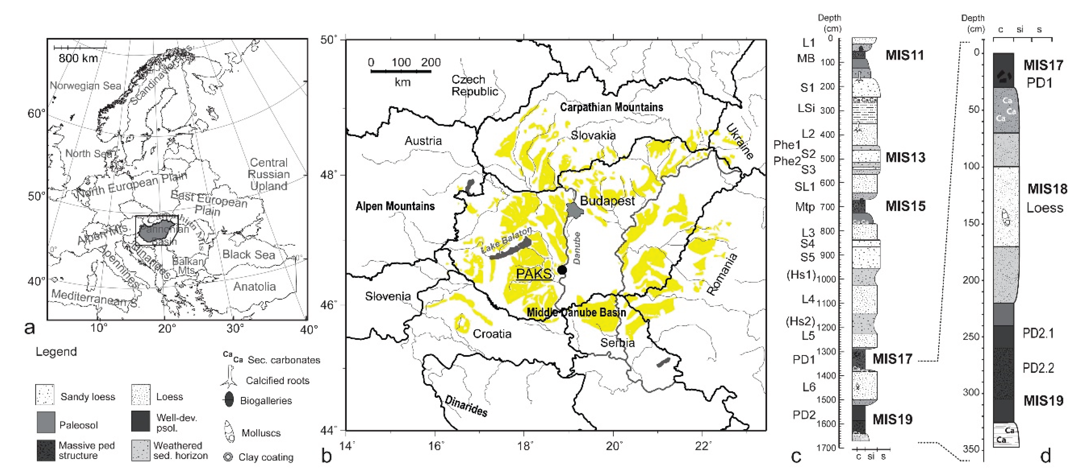
Figure 2.
The stratigraphy of the studied part of the Paks succession and related susceptibility curves, such as a.) low field magnetic susceptibility measured in the field (5-cm measuring interval), b.) low field mass susceptibility measured in the laboratory with a 5-member running average curve (~2 cm sampling interval), and c.) absolute frequency dependence measured in the laboratory. The legend of the stratigraphic graphic log of the section follows Figure 1.
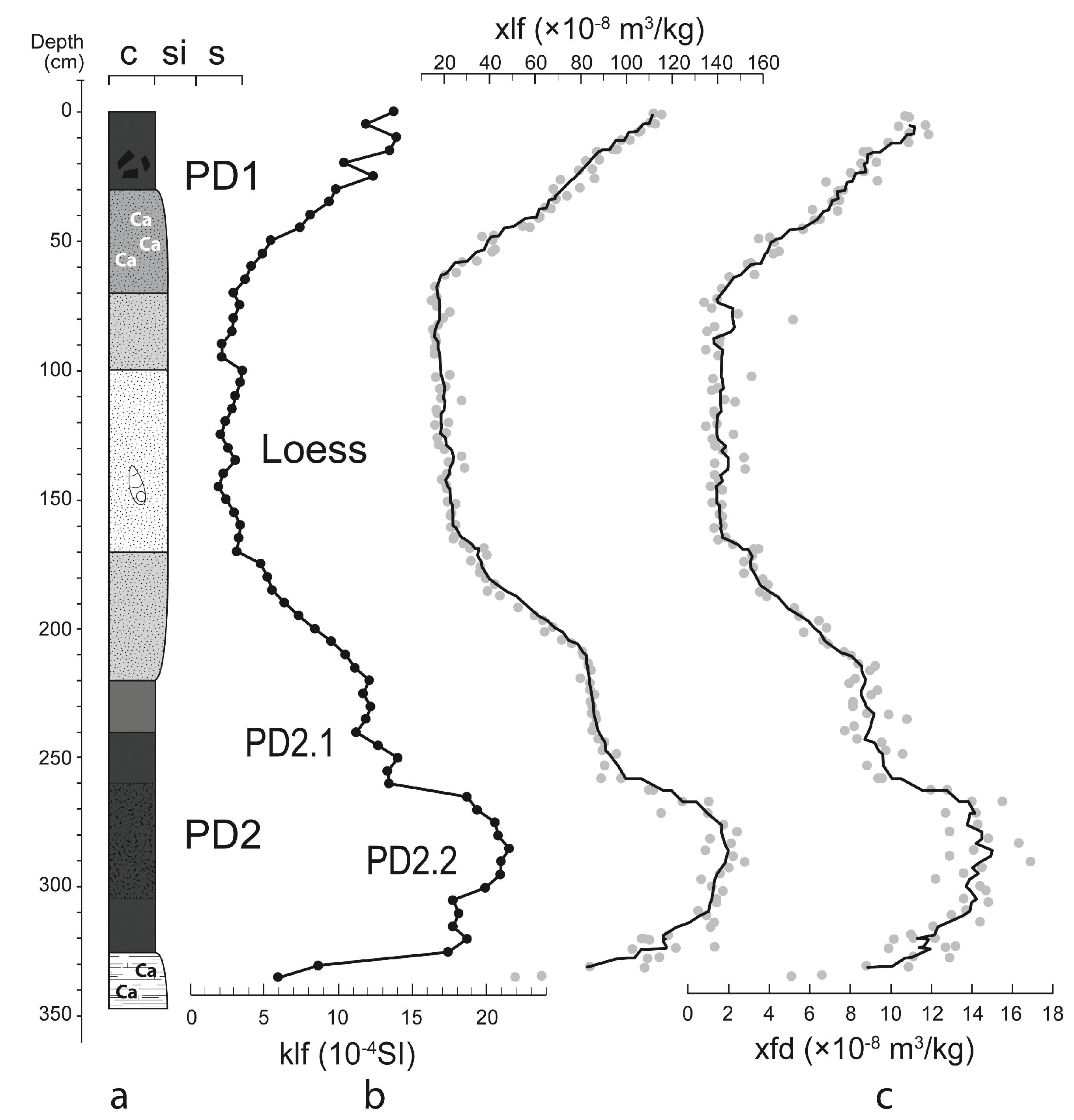
Figure 3.
The summary of various magnetic susceptibility measurements. The box and whisker plot of the basic anisotropy parameters (a, b, and c). The boxes denote the interquartile range, whereas data falling within 1.5 times the value of the interquartile range are represented by the two T-bars (the lower and upper whiskers). Asterisks mark the average, and the black line within the box shows the median [40]. ꭓlf to ꭓfd plot (d) indicates the pedogenic origin of the superparamagnetic components, increasing with the degree of pedogenesis.
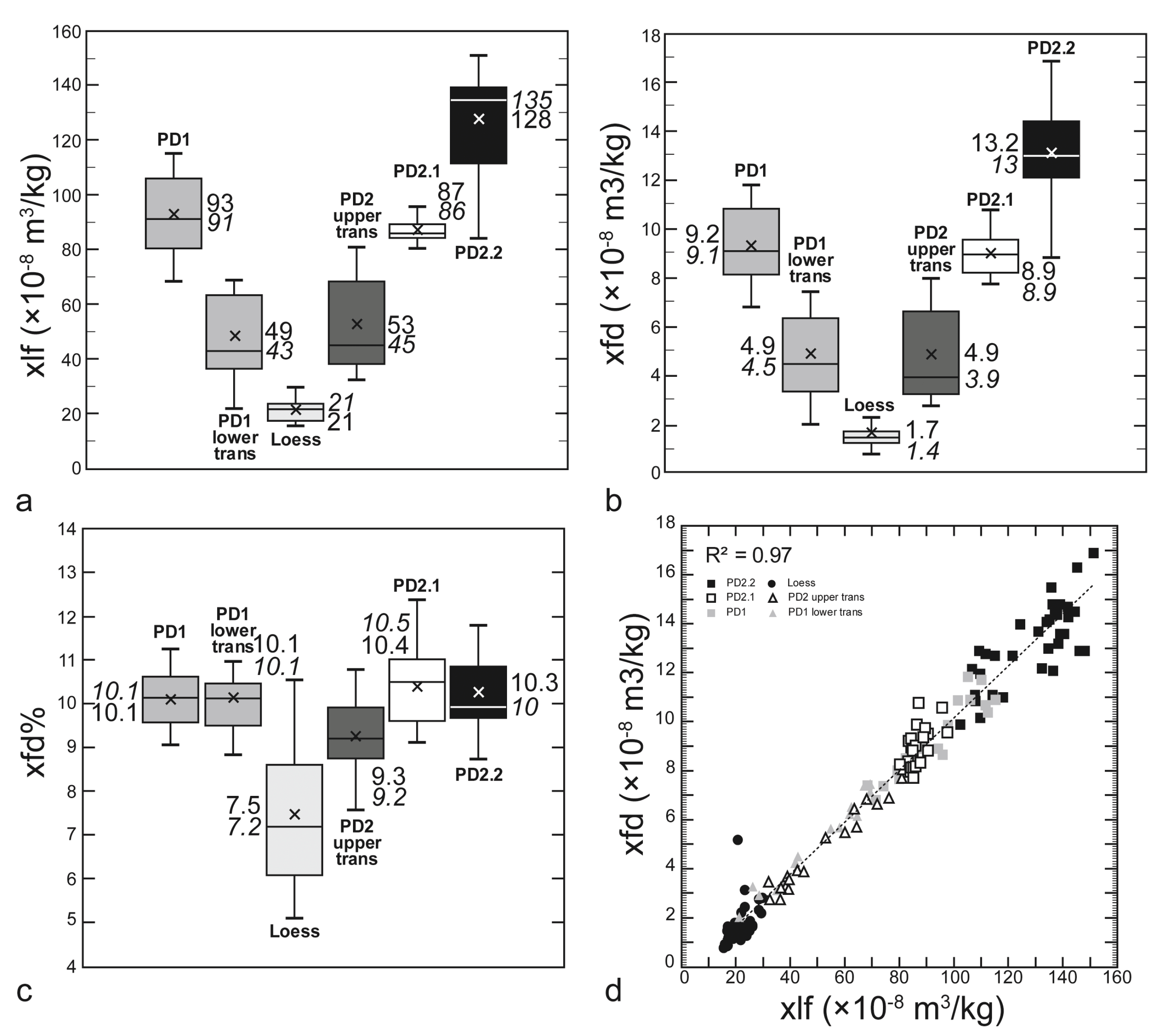
Figure 4.
Temperature variation in magnetization identified by normalized heating (solid) and cooling curve (dotted) of samples from the overlaying loess (a) of the PD2.1 (b) and PD2.2 (c and d) paleosol units. The colored curves represent the running average (5-member) of the original data (gray curves). Red curves and arrows indicate the heating cycles, and red curves and dotted arrows represent the magnetization change during cooling.
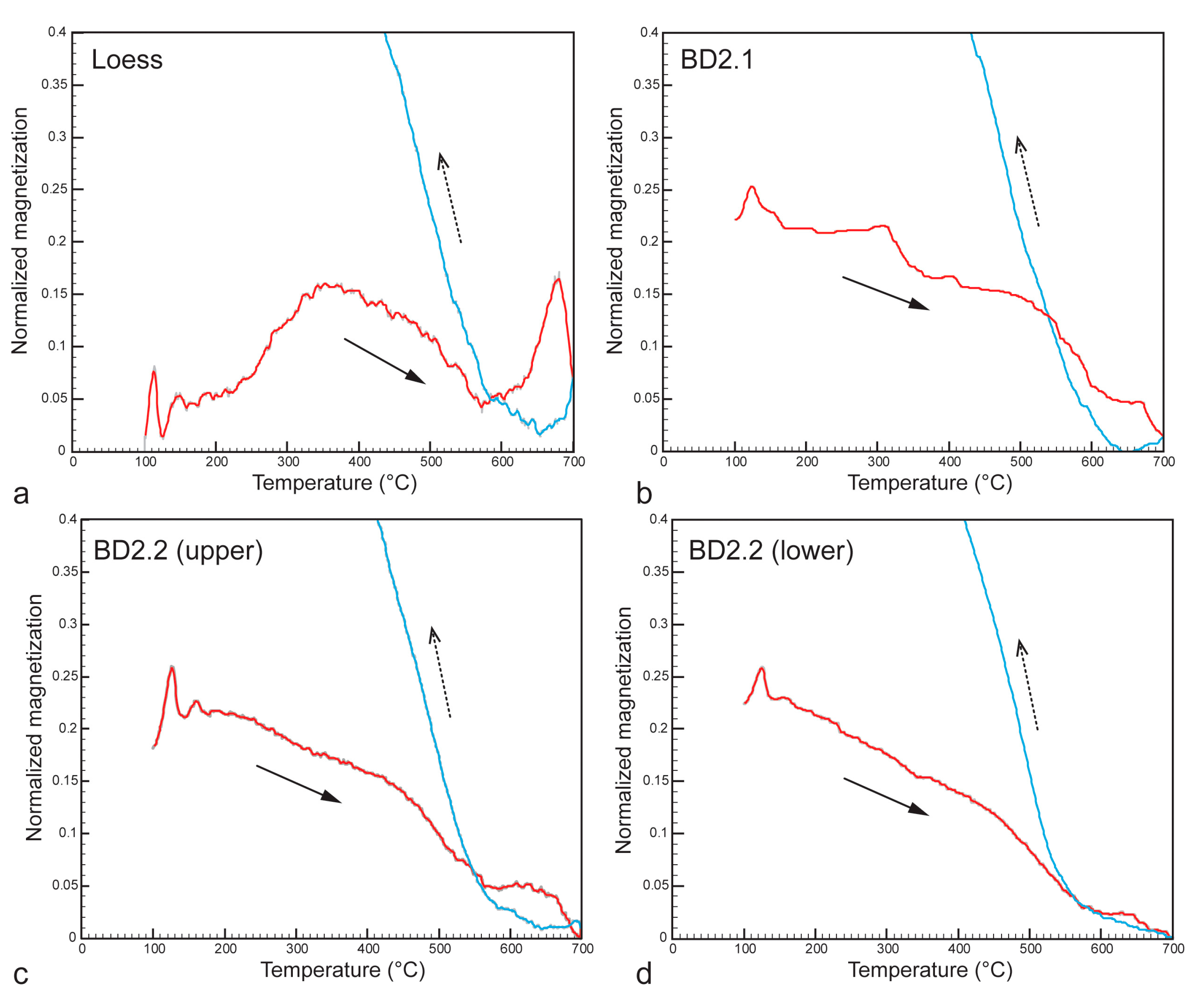
Figure 5.
Representative AFD and ThD (Zijderveld) diagrams from the normal polarity (a, b), reversal polarity (c, d), and transition zone (e) in the Paks profile.
Figure 5.
Representative AFD and ThD (Zijderveld) diagrams from the normal polarity (a, b), reversal polarity (c, d), and transition zone (e) in the Paks profile.
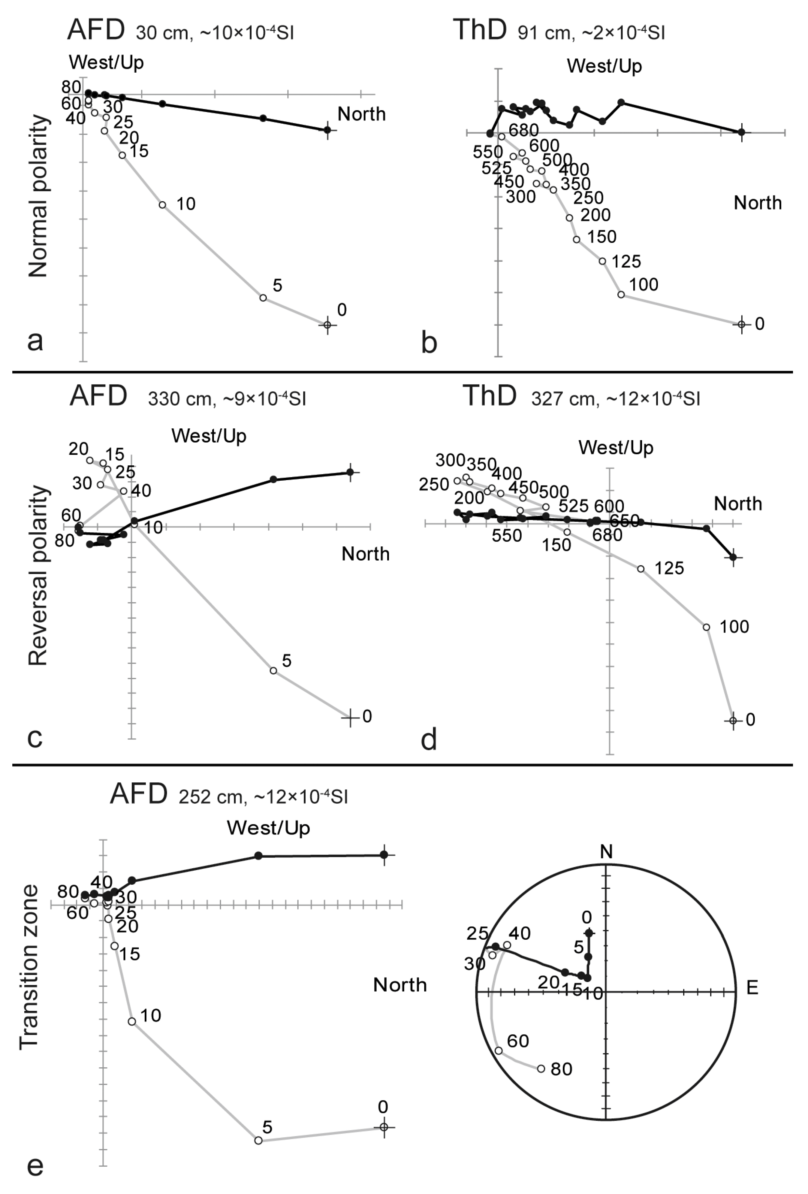
Figure 6.
Stratigraphic plots of the magnetic results: a.) the low field magnetic susceptibility; b.) the inclination of ChRM separated by AFD and ThD; c.) the declinations (AFD-gray; ThD-black); d.) the latitude and e.) longitude of VGP (virtual geomagnetic pole); and f.) maximum angular deviation (MAD) values. The results of AFD are represented by gray and black curves, which represent the results from ThD. The small dots (gray-AFD, black-ThD) represent the samples that did not show ChRM during the analysis.
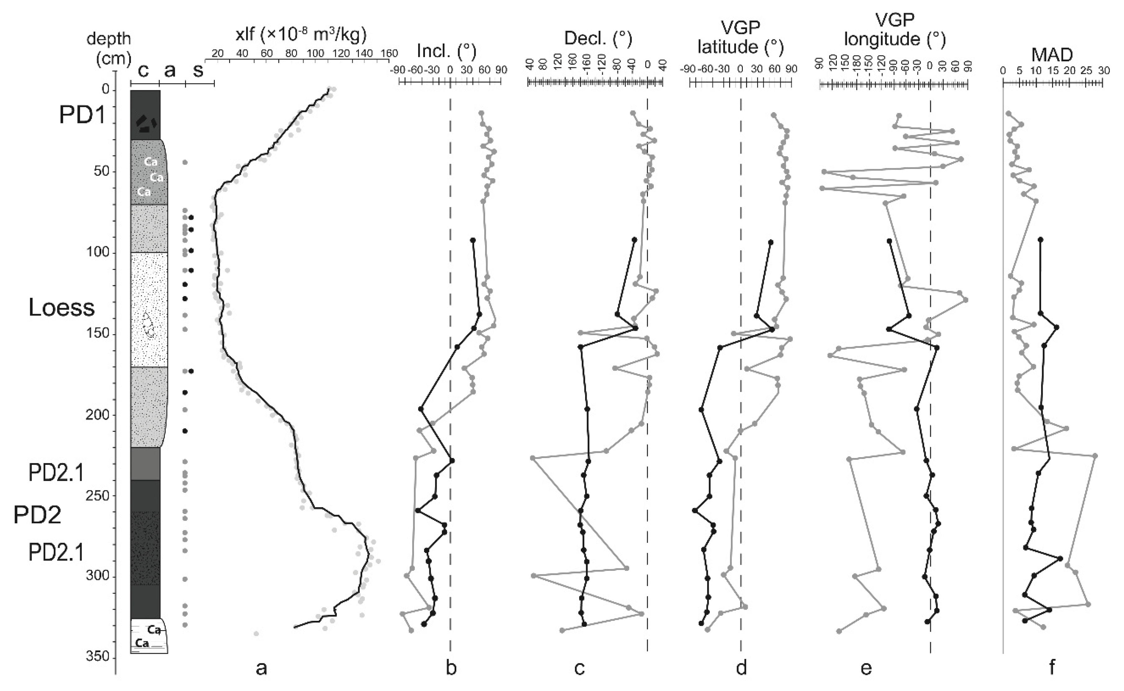
Figure 7.
The stratigraphic position of the Matuyama-Brunhes Transition (MBT) in the Paks succession (a). The comparison of the behavior of the geomagnetic field, characterized by RPI records of the section (a, c) to the RPI of the Osaka Bay sequence [46] (d) and to the Virtual Axial Dipole Moment (VADM) by Guyodo & Valet [47] (e). The gray curves indicate the calculated RPI based on the NRM measured at 30 mT demagnetization field normalized by the ꭓlf (b) and the anhysteretic remanent magnetization (ARM) at 30 mT.
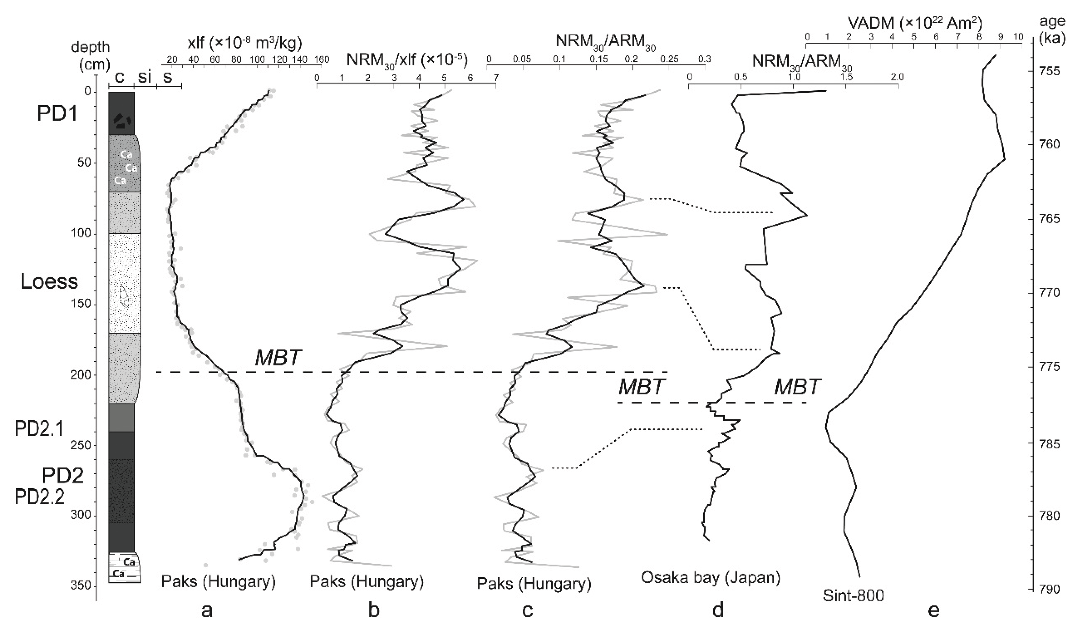
Figure 8.
Describing potential paleoclimatic and paleoenvironmental drivers and their effects on the formation of paleosols and sedimentation of loess around the MBT. A.) the strength of the geomagnetic field, b.) the relation between the putative unusual cooling event (triggered by e.g. the Umbrella-effect) and the influence of ‘regular’ rhythm of the interglacials and glacials, c.) the changing intensity of pedogenesis (indicated by magnetic susceptibility) and d.) the changing relationship between pedogenesis and sedimentation. The arrows with dashed lines indicate a weak and weakening geomagnetic field, and the black arrow indicates strengthening (Figure 8a). The grey arrows indicate pedogenesis, and the arrows with ‘loess’ texture indicate sedimentation. The size of these arrows indicates the degree of the process and the balance between pedogenesis and sedimentation (Figure 8d).
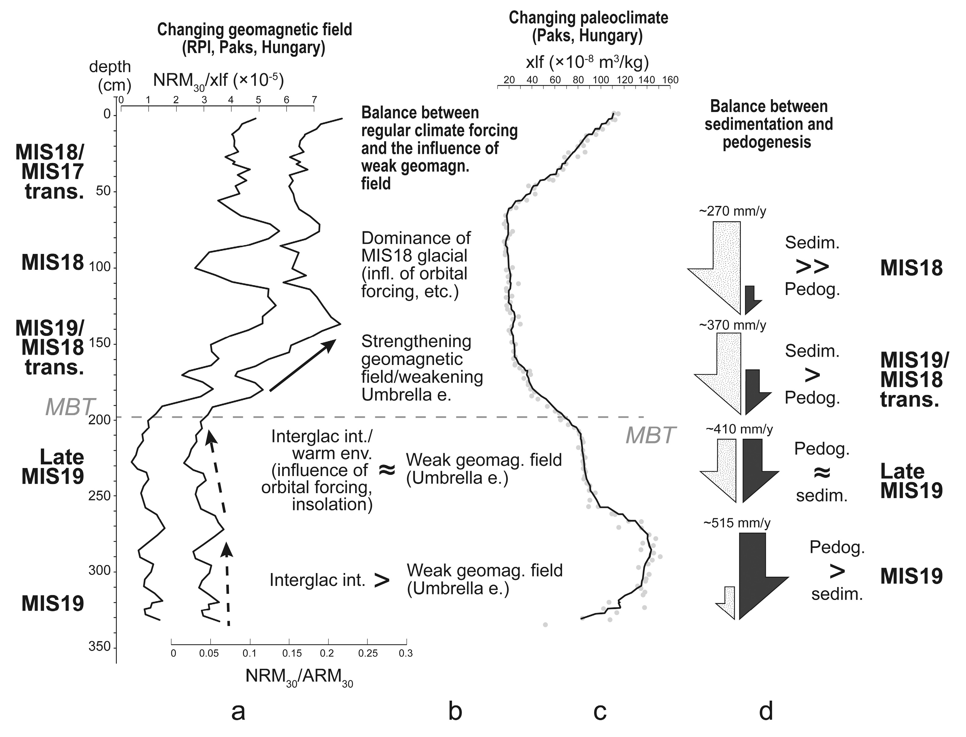
Table 2.
Possible marks of the cooling event on the susceptibility curves representing the MBT and MIS 19 at some loess profiles from Eurasia (literature review). Abbreviations: European Loess Belt – ELB; including the Middle Danube Basin – MDB; Lower Danube Basin – LDB; Eastern European Plain – EEP; and Chinese Loess Plateau – CLP.
| Site | Characteristics of the MBT/MIS19 units (mag. sus. curve) | Ref. | ||
|---|---|---|---|---|
| European Loess Belt | Červený Kopec | No clear marks of the cooling event | [25] | |
| NW of EEP | Koriten | No clear marks of the cooling event (small peaks representing the MIS19 paleosol) | [56] | |
| Viatovo | Smaller peaks on the local maxima of MIS19 paleosol (similar to Xifeng, CLP) | [56] | ||
| Central Danube Basin | Paks | A step-like feature on the local maxima of MIS19 paleosol | ||
| Novaya Etuliya | No clear marks of the cooling event | [31] | ||
| Stari Slankamen | Smaller peaks and a thick upper transition horizon on the local maxima of the MIS19 paleosol (similar to Chaona and Chanwu). | [29] | ||
| LDB | Zimnicea | A step-like feature on the local maxima of the MIS19 paleosol | [57] | |
| Korolevo | No clear marks of the cooling event (narrow peak representing the MIS19 paleosol) | [30] | ||
| SW of EEP | Roxolany | Sharp boundary between the MIS19 paleosol and the overlaying loess (abrupt change in the climate or hiatus) | [31] | |
| Zahvizdja | No clear marks of the cooling event | [30] | ||
| Dolynske | A step-like feature on the local maxima of the MIS19 paleosol | [33] | ||
| Central Asia | Darai Kalon | A step-like feature on the local maxima of MIS19 paleosol | [58] | |
| Karamaidan | A step-like feature on the local maxima of MIS19 paleosol (not a characteristic appearance) | [59] | ||
| East Asia (CLP) | Chaona | Smaller peaks and a thick upper transition horizon on the local maxima of MIS19 paleosol (similar to Stari-Slankamen and Chanwu) | [60] | |
| Chanwu | Smaller peaks and a thick upper transition horizon on the local maxima of MIS19 paleosol (similar to Stari-Slankamen and Chaona) | [61] | ||
| Lingtai | A step-like feature on the local maxima of the MIS19 paleosol | [62] | ||
| Luochuan | Thick upper transition horizon (similar to Chanwu) | [34] | ||
| Xifeng | Smaller peaks and a thick upper transition horizon on the local maxima of the MIS19 paleosol (similar to Chanwu and Luochuan). | [62] | ||
| Zhaojiachuan | A step-like feature on the local maxima of the MIS19 paleosol | [34] | ||
Disclaimer/Publisher’s Note: The statements, opinions and data contained in all publications are solely those of the individual author(s) and contributor(s) and not of MDPI and/or the editor(s). MDPI and/or the editor(s) disclaim responsibility for any injury to people or property resulting from any ideas, methods, instructions or products referred to in the content. |
© 2025 by the authors. Licensee MDPI, Basel, Switzerland. This article is an open access article distributed under the terms and conditions of the Creative Commons Attribution (CC BY) license (http://creativecommons.org/licenses/by/4.0/).
Copyright: This open access article is published under a Creative Commons CC BY 4.0 license, which permit the free download, distribution, and reuse, provided that the author and preprint are cited in any reuse.


