

Submitted:
06 August 2025
Posted:
11 August 2025
You are already at the latest version
Abstract
This article explores the impact of weather and environment on shared bicycles. Using a random forest model combined with explanatory machine learning methods, the relationship, threshold effect, and interaction effect between weather factors and the transfer volume of shared bicycles at subway stations are analyzed; Based on the spatial Durbin model, analyze the relationship between the transfer volume of shared bicycles and factors such as the built environment. Research has shown that there is a significant non-linear relationship between various weather factors and the transfer volume of shared bicycles; Temperature, humidity, and rainfall have specific activation and threshold effects on the number of shared bicycle transfers. Population statistics, socio-economic factors, building environment, road environment and other characteristic variables have a significant impact on the shared bicycle transfer volume in each study area and adjacent study areas under adverse weather conditions, indicating that factors such as built environment have a spatial spillover effect on the shared bicycle transfer volume.
Keywords:
green mobility
; shared bikes
; transfer volume
; interaction effect
; interpretable random forest model
1. Introduction
With the increasing urban population and the escalating issue of traffic congestion, shared bikes have emerged as a crucial solution to enhance travel efficiency and alleviate traffic pressure [1]. Shared bikes not only reduce the travel volume of private cars and enhance the attractiveness of public transportation but also effectively decrease motor vehicle emissions and energy consumption, playing a positive role in improving urban environmental quality and addressing climate change [2]. Additionally, as a flexible and convenient mode of short-distance travel, shared bikes serve as an important choice for transferring to the subway. The combined use of shared bikes and subways has become a significant mode of transportation for commuters. Typically, individuals opt for shared bike rides to reach subway stations in close proximity, followed by subway rides to stations near their destinations. During this journey, shared bikes play the role of the starting point for travel activities. When commuters arrive near their destinations from subway stations, shared bikes serve as the “last mile” solution, providing quick and convenient transfer services [3,4], acting as the endpoint for travel activities. Presently, the combined use of shared bikes and subways is widely adopted in densely populated major cities. For instance, in the total shared bike travel volume in Shanghai, China, 51% of shared bike travel occurs near subway stations [5].
However, shared bike travel is exposed to external environmental conditions and is susceptible to factors such as temperature, rainfall, and air pollution [6,7]. The external environment has become a key influencing factor for travelers in choosing the combined use of shared bikes and subways. Despite the increased flexibility of shared bikes compared to private bikes, for example, allowing on-the-spot parking in rainy weather [8], the use of shared bikes still faces certain obstacles. There exists a complex relationship between shared bike travel and weather factors, making shared bike users more vulnerable to the effects of weather changes. Previous studies indicate that, compared to driving and using public transportation, shared bike travel is more sensitive to weather variations. Therefore, gaining a deeper understanding of the impact of weather conditions on shared bike travel and the extent of this impact is crucial for grasping the usage patterns of shared bikes under different weather conditions, promoting the combined use of shared bikes and subways, alleviating urban traffic congestion, and reducing carbon emissions.
While existing studies have explored the impact of weather on bike travel [9,10,11], research on the influence of weather on shared bike travel is relatively limited, with even fewer studies focusing on the impact of weather on shared bike transfer volume. In this study, a buffer zone is established centered around subway stations, treating the buffer zone as an area for parking shared bikes when transferring to the subway. The number of shared bike orders ending their journeys within the boundary of this buffer zone is defined as the shared bike transfer volume, serving as the subject of investigation in this study. By integrating data from multiple sources, including subway route information, station geographic data, meteorological data, and air quality index, we conduct a comprehensive study on the impact of weather on the combined use of shared bikes and subways. This extends the scope of previous research on shared bike travel behavior.
It is noteworthy that many studies on the impact of weather on shared bike transfers commonly employ traditional parameter models and linear assumptions. Although these studies can indicate the influence of weather on shared bike transfers, the traditional parameter models and linear models often generate biased estimates and inaccurate interpretations due to the neglect of nonlinear effects and interactions among relevant weather factors [12]. For instance, there may be an interaction between humidity and temperature, where changes in humidity can enhance or diminish the impact of temperature. Additionally, the relationship between temperature and shared bike transfer volume may exhibit nonlinear characteristics with certain thresholds [13]. In order to comprehensively explore the nonlinear effects of weather on shared bike transfers, this study adopts a random forest model and interpretable machine learning methods. This approach expands the nonlinear analysis methods for shared bike transfer volume, providing robust support for the interpretation of the nonlinear effects of weather factors on shared bike transfer volume. At the same time, based on the spatial Durbin model, the relationship between the change rate of shared bicycle transfer volume and factors such as the built environment is analyzed, and the spatial correlation of the change rate of shared bicycle transfer volume and the influence of factors such as the built environment are explored to determine whether there is a spatial spillover effect.
2. Literature
2.1. Combined Travel Between Shared Bikes and Subway
Shared bikes, serving as a short-distance travel solution for addressing the “last mile” problem in urban transportation, naturally complement long-distance commuting modes such as the subway. Consequently, numerous studies have explored the integrated use of shared bikes and subway systems. Noland et al. found that shared bike stations near subway stations have higher utilization rates, emphasizing the comprehensive use of shared bikes and subways [14]. Guo et al. using subway daily passenger volume as the independent variable and employing negative binomial regression, identified a positive correlation between subway passenger volume and the volume of shared bike travel [15]. Some literature has constructed a fusion evaluation index for subways and shared bikes, utilizing a generalized additive model to investigate the correlation between this index and land use, social demographics, road design, and transportation facilities [16]. Zhan et al. extracted shared bike data near subway stations and employed local cumulative effect maps to analyze factors related to the integrated use of shared bikes and subways, identifying subway passenger flow and bike density around the service area as the most crucial factors promoting shared bike use near subway stations [17]. Yan et al. extracted data on dockless shared bikes near Shanghai Metro Line 9, visually analyzing the differences in usage patterns of dockless shared bikes around subways on weekdays and weekends, revealing characteristics of dockless shared bike service areas around subways [18]. Data from the Nanjing Metro in China indicated that the coverage area of subway stations determines the demand for the integrated use of shared bikes and subways. Subway stations with higher density reduce the potential for integrated use since shared bikes can be replaced by walking as a connection to the subway [19]. In summary, over the past few years, the combined use of shared bikes and subways has experienced significant growth in many regions, representing one of the most important future directions for the development of shared bikes. Therefore, it is necessary to explore the factors influencing commuters’ choices in adopting the combined use of shared bikes and subways.
2.2. The Impact of Weather on the Use of Shared Bikes
Previous research has revealed that weather factors significantly impact the use of shared bikes, leading to several scenarios: commuters opting for alternative transportation modes to avoid the effects of weather, delaying their departure until unfavorable weather conditions pass, or choosing not to travel to avoid weather impacts [20]. Therefore, it is crucial to incorporate weather factors into the impact system of shared bike travel. This can be achieved by collecting shared bike road count or order data, along with meteorological data, and conducting modeling and analysis from both temporal and spatial perspectives [21,22], to explore the impact of weather factors on shared bike travel behavior. El-Assi constructed an autoregressive moving average model to estimate shared bike travel volume, finding that warmer weather leads to higher shared bike utilization rates, while rainfall, low temperatures, and humidity decrease utilization rates [23]. Additionally, Wessel studied the influence of predicted weather conditions on cycling volume, revealing that even during rainless periods, predicted rainfall reduces cycling volume by 3.6% [24].Gebhart analyzed shared bike data and discovered that shared bike travelers embarking on journeys farther from subway stations are more susceptible to the impact of rain and low temperatures compared to those starting journeys closer to subway stations [25]. Currently, the combined use of shared bikes and subways constitutes a significant proportion of overall shared bike travel. However, research on the impact of weather on the combined use of shared bikes and subways is relatively scarce. This study explores the influence of weather on the transfer volume between shared bikes and subways, aiming to identify explanatory methods for the impact of weather on shared bike and subway transfer volume. This research holds guiding significance for the study of the combined use of shared bikes and subways.
3. Research Area and Data
3.1. Study Area
The selected study area for this research is Washington, D.C., located in the Mid-Atlantic region on the East Coast of the United States, at the border between the states of Maryland and Virginia. Washington, D.C. stands as one of the earliest cities in the United States to introduce shared bikes, with a system operational for over 14 years. Capital Bikeshare (CaBi) operates the shared bike system in this region, boasting over 6,000 shared bikes and more than 700 bike docking stations in Washington, D.C. as of December 2023. Additionally, the region is well-served by an extensive rail transit system, with Washington Metro ranking second only to the New York City subway in terms of passenger volume. As of December 2023, Washington Metro operates six subway lines and 97 stations. Under the planning and development initiatives of the transportation management authorities in the region, the urban shared bike system in Washington, D.C. has gradually emerged as a significant mode for transferring to the city’s rail transit system. The study area, locations of shared bike docking points, and subway routes used in this research are illustrated in Figure 1.
3.2. Data Source and Description
This study explores the influence of weather factors on the number of shared bike transfers, using a dataset that contains the following categories: (1) numerical air pollutant data for Washington, D.C., U.S.A., for the year 2022, published on the World Air Quality Index (WAQI) website, with a representative air pollutant selected as PM2.5, and the raw data structure of PM2.5 concentration contains the monitored in a day’s minimum, maximum, median, standard deviation, and number of measurements; (2) historical data on the UV index for the region published on the National Oceanic and Atmospheric Administration (NOAA) website, where the UV index is a converted grade and the UV index grade is in the range of 0 -11; (3) data on the air pollutant values for Washington, D.C., U.S.A., for the year 2012 published on www. rp5.ru website published the historical weather data of the Ronald Reagan Washington National Airport weather station in Washington, D.C., mainly including temperature, visibility, humidity, wind speed, rainfall, etc., which were recorded every three hours; (4) OpenStreetMap (OSM) platform published map information data collected in this study mainly includes city administrative area data, rail transit line network and station data; (5) the bike sharing order data published by Capital Bikeshare after hiding users’ personal information, the data structure contains user number, station name and its latitude and longitude, latitude and longitude of the starting point and the ending point, departure time and ending time, user type and bike type, etc. The time span of the above original datasets is from January 2022 to December 2022, and the sources and descriptions of the datasets are shown in Table 1.
3.3. Study Variables
3.3.1. Extraction of Bike-Sharing Order Data near Subway Stations
In order to extract shared bike order data near subway stations, this study utilized ArcGIS geographic processing software. Washington, D.C. subway station location information was imported, and buffer zones were set to extract shared bike order data that matched the locations within these buffers. However, there is no unified standard for determining the radius of the buffer zone, which may be related to factors such as the distance of subway stations from the city center, subway service capacity, population density, and the composition of surrounding users [26]。Referencing previous scholars’ research [2,3,4,5], this study introduced the method of spatial network density to determine the range of buffer zones around subway stations. Firstly, the method assumed that subway stations have a certain attractiveness to nearby shared bikes, forming a buffer zone. As the radius of the buffer zone increases, the density of shared bike orders within this range would initially increase and then decrease.
Therefore, based on this fundamental assumption, the study needs to establish a function for the variation in shared bike order density near subway stations. Given that Washington, D.C. has a dock-based shared bike system where bikes must be parked at designated stations, for simplification, this study substituted shared bike station density for shared bike order density. The calculation formulas are shown in Equations (1) and (2):
In the equations, represents the spatial density change function of public bike stations near subway station k,with a buffer zone radius of . is the minimum search step, set to 100m in this study. is the number of shared bike stations within the maximum buffer zone R, where R is set to 1000m in this case. is the Euclidean distance from shared bike stations to subway station k, is an indicator function. The distribution of values for various subway stations under different buffer zone radii is shown in Figure 2(a) as a boxplot, with point data representing the spatial density of stations for each subway station. Due to the relatively large minimum search step, the phenomenon of increasing and then decreasing spatial density of public bike stations was not observed. However, it can be observed that when the buffer zone radius expands to 500m, the mean and variance converge. Therefore, this study sets the buffer zone distance for subway stations to 500m. Figure 2(b) displays the kernel density analysis results for shared bike orders near McPherson Square subway station, confirming the 500m buffer zone as it effectively covers the hotspots of shared bike station distribution.
3.3.2. Dependent Variable
Based on the analysis in Section 3.3.1, this study has successfully extracted all the stations from the Washington Metro rail lines and established a buffer zone with a radius of 500m. This buffer zone serves as the area where users of shared bikes choose to park their bikes when combining shared bikes with subway travel. In this study, the quantity of shared bike orders that conclude their trips within this buffer zone is defined as the shared bike transfer volume. This variable is set as the dependent variable for the study of combined travel using shared bikes and the subway.
Through the batch processing function of the ArcGIS model builder, 1.04 million shared bike orders in the buffer were extracted, and these shared bike interchanges accounted for one-third of the total shared bike trips. After data cleaning, the spatial and temporal distribution characteristics of the shared bike interchanges are obtained, as shown in Figure 3.
Figure 3a shows the trend of shared bike interchange and total shared bike trips for the whole year of 2022. As can be seen from Figure 3a, the year-round trend of shared bike interchange is more gently distributed than total trips, which indicates that shared bike interchange has formed a stable demand at metro stations and has become one of the main modes of interchanging to the metro. Figure 3b shows the trend of shared bike transfer volume in 24 hours a day, and there is an obvious phenomenon of morning and evening peaks in shared bike transfer volume. Figure 3c shows the hotspot distribution area of the shared bike transfer volume, and it can be clearly seen that the density of shared bike transfer hotspots in downtown metro stations is much higher than that in suburban areas.
3.3.3. Independent Variables
In order to deeply explore the influence of weather factors on the amount of bike-sharing interchange, this study integrates five data sources and K-Means cluster analysis methods to build a three-category weather variable framework to study the role of weather factors on the combination of bike-sharing and subway trips. The input variables are mainly three categories: basic weather variables, virtual weather variables, and weather forecast variables, and the statistical descriptions of these input variables are shown in Table 2.
(1) Basic weather variables
In previous studies, numerous scholars have found that environmental factors such as temperature and rainfall have a significant impact on bike travel [15,30,31]。Therefore, in this study, temperature, humidity, visibility, wind speed, rainfall, and values of UV index and air pollutants from January 2022 to December 2022 were included in the study, and they were considered as the underlying weather variables. Since some of the original environmental statistics are minute-by-minute, hour-by-hour, and day-by-day data with inconsistent data statistical intervals, the base weather variables were homogenized in this study.
(2) Dummy weather variable
In order to investigate the influence of unfavorable weather on bike-sharing interchange, this study constructs a virtual weather variable based on the basic weather variable, which contains six kinds of dry, humid, low temperature, strong wind, rainfall and strong ultraviolet rays. The virtual weather variables are dichotomous variables with values of 0 and 1. Due to the selection method of the virtual weather variables, there are mainly two kinds of definitions, absolute value definition and relative value definition, absolute value definition refers to the method of taking a fixed value, e.g., defining the temperature lower than 0℃ in a day as low temperature weather; relative value definition is to take a percentile method, e.g., arranging the temperature values according to the size and taking the value in the lowest 20% of the values. portion is defined as cold weather [32,33,34,35]. These two selection methods of virtual weather variables have their own advantages. However, they still cannot accurately reflect the specific nodes of the changes in the characteristics of the virtual weather variable observations. In this study, the basic weather variable data were divided into five categories, and the K-Means clustering algorithm shown in Equations (3) and (4) was introduced to solve the clustering centers by minimizing the variance within the same cluster, maximizing the cluster distances of different clusters, and solving the cluster center values, and then, the highest or lowest cluster center value is selected as the boundary center value for dividing the virtual weather variables.
Where k denotes the number of clusters, is the average value of observation x in class , also called the cluster center value. E is the sum of error squares, the smaller the value means that the observation x is closer to the cluster center, the better the clustering effect. After the iterative calculation of K-Means clustering algorithm, the clustering results of virtual weather variables shown in Table 3 are obtained. Among them, the observed values of rainfall are clustered into 3 major categories, and the rest of the virtual weather variables are clustered into 5 major categories. Based on the K-Means clustering results shown in Table 3, this study defines the Type I and Type V samples of humidity as dry weather and wet weather, respectively; the Type I samples of temperature as cold weather; the Type V samples of wind speed as wind weather; the Type III samples of rainfall as rainy weather; and the Type V samples of UV intensity as strong UV weather.
(3) Weather forecast variables
Most of the previous studies only consider the effects of historical weather or real-time weather on bike sharing ridesharing, but in real life, travelers often also refer to the weather forecast when planning their trips and deciding on their future travel modes. [36]. Since unfavorable weather events such as low temperatures, strong UV rays and rainfall can have a prospective impact on bike-sharing interchange, it is necessary to include low temperature forecasts, UV warnings and rainfall forecasts as weather forecast variables in this study.
4. Research Methods
4.1. Random Forest Model
Random Forest (RF) algorithm is a classical ensemble learning method and an extension of Bagging. It further introduces random attribute selection into the training process of decision trees, building on the foundation of constructing a Bagging ensemble with decision trees. Compared to traditional regression models, RF has several advantages. Firstly, RF exhibits a certain degree of robustness as it imposes no restrictions on the type of input variables, they can be numerical, categorical, continuous, or discrete. Moreover, RF is insensitive to skewed distributions, outliers, and noisy data. Secondly, RF requires relatively fewer hyperparameter tuning. The main hyperparameters include the number of decision trees, the maximum number of features to consider when constructing a decision tree, and the maximum depth of the decision tree. These hyperparameters are not very sensitive to their values. Importantly, RF, as a tree-based ensemble learning algorithm, possesses strong nonlinear fitting capabilities due to its flexible modeling structure. It can automatically learn the correlation and weight distribution among input features, model complex nonlinear relationships between input variables and response variables, and capture high-order interactions between variables.
In recent years, some progress has been made with the Interpretable Machine Learning (IML) [37], the combination of IML and Random Forest (IML+RF) has found widespread applications in the field of transportation, serving various purposes such as predictions and data interpretation. For instance, RF has been employed for short-term forecasting of bus passenger volumes, and IML has been utilized to assess the influencing factors on bus travel speeds [38,39]. Additionally, RF has been used to establish regression models between pollutant concentrations, while IML has been applied to analyze the relative importance of variables such as meteorological conditions, time factors, and traffic flow [40]. This suggests that employing IML+RF for the analysis of shared bike transfer volumes is feasible. Therefore, this study first utilizes RF to establish a regression model for shared bike transfer volumes based on comprehensive weather variables. Subsequently, employing IML algorithms for feature interactions, feature importance ranking, and cumulative local effect plots, the study interprets the results of the regression model.
4.2. Model Interpretability
4.2.1. Feature Interaction
There may be interactions between weather factors, and when exploring the effect of weather on bike-sharing to subway, it is not possible to consider only the sum of the effects of each part of the weather variables, this is due to the fact that the effect of the influence of one weather variable is often also dependent on the value of another weather variable. Therefore, this study will explore the interaction effects between weather variables using Feature Interaction from the IML package. Feature Interaction was proposed by Friedman and Popescu [41] and is based on H-statistic. The H-statistic value is based on the underlying theory of decomposition of the partial correlation function, which is defined as function that depends only on the characteristics of and as well as the interaction between the and characteristics, and when the two characteristics do not interact with each other, the partial correlation function can be decomposed into the form of Equation (5):
When there is an interaction between two features, the H-statistic value for assessing the strength of the interaction is calculated by Equation (6):
where is the bi-directional partial correlation function of the two features J and K,and are the partial correlation functions of the individual features.
4.2.2. Importance of Features
To elucidate the impact of weather factors on shared bike transfer volumes, this study introduces the parameter of feature importance, utilizing it to assess the significance of weather factors. Feature importance is gauged by calculating the variation in model prediction errors based on changes in feature values. If altering a particular feature value leads to an increase in the model’s prediction error, the feature is deemed “important” [42,43]. conversely, if the error decreases, the feature is considered “unimportant.” In contrast to linear regression models, which only reflect the significance levels of variables, feature importance comprehensively considers both main effects and interaction effects of feature variables. It ranks the importance of feature variables, providing policymakers with deeper insights when seeking intervention measures.
4.2.3. Accumulated Local Effects Plot
The Accumulated Local Effects plot (ALE) is commonly used to illustrate how explanatory variables influence the predictions of a machine learning model. In comparison to Partial Dependence Plots (PDP), ALE plots serve as a faster and unbiased alternative. PDP assumes that all explanatory variables are independent, making it unsuitable when strong correlations exist among explanatory variables. In this study, since weather factors are the explanatory variables and there is substantial correlation among most weather factors, PDP is not suitable. Therefore, ALE plots are considered a feasible explanatory tool for weather variables in this research.
4.3. Spatial Durbin Model
The spatial Durbin model [20] is a type of spatial econometric model; The spatial econometric model is developed on the basis of non spatial linear regression models, expanding into models with spatial interaction effects by adding spatial lag and random error terms. The spatial model composed of this extension method separates the impact of spatial interactions on research data, which can more accurately describe the spatial effects between data. In spatial econometric models, the spatial lag term is used to represent the interaction between the variables of a geographic unit and the variables of its adjacent geographic units. This spatial effect includes spatial autocorrelation, spatial spillover, and so on. By introducing spatial lag terms, we can better explore the mutual influence between adjacent geographic units, thereby gaining a more comprehensive understanding of the spatial structure of the data. At the same time, the spatial econometric model also takes into account the spatial error term, which is used to capture the impact of unobserved spatial factors on the dependent variable in the model. These unobserved spatial factors may lead to spatial correlation between the residuals of the model. Therefore, introducing a spatial error term can better control this spatial correlation, improve the fitting degree and predictive ability of the model.
The non spatial linear regression model between environmental factors and the rate of change in shared bicycle transfer in this chapter can be expressed as:
Y=α+X β+ε
In the formula, Y represents the change rate of shared bicycle transfer volume under adverse weather conditions in a certain area; α is a constant, which is an N × 1 order vector; X is an independent variable such as the built environment, which is an N × K order matrix, where K is the number of variables such as the built environment; β is the regression coefficient corresponding to the independent variable, which is a K × 1st order vector; ε is the standard error term, which is an N × 1 order vector and ε~N (0, σ 2).
The spatial lag and spatial error models have their own limitations, as both models limit the degree of spatial effects; In addition, both did not consider local and global spillover effects, which may seriously interfere with the interpretation of model results. To solve this interference problem, this article introduces the spatial Durbin model for analysis, which is expressed as:
Y=α+ρWY+Xβ+WXθ+ε
In the formula, W is the spatial weight matrix. This chapter establishes the spatial weight matrix of each geographical unit based on whether the research areas are adjacent or not; ρ and θ are unknown parameters that need to be estimated, commonly referred to as spatial autoregressive coefficients; WY can be understood as the endogenous interaction effect between the change rates of shared bicycle transfers in different regions, while WX is the exogenous interaction effect between variables such as the built environment in each region.
The above spatial Durbin model considers the combination of exogenous and endogenous interaction effects of the change rate of shared bicycle transfer volume in different regions under adverse weather conditions by adding spatial lag terms for the dependent variable Y and the independent variable X. Due to the fact that spatial Durbin models do not limit the size of spatial interaction effects, they generate unbiased coefficient estimates and do not result in misclassification of spatial effects. From indicators such as maximum likelihood estimation and Akashi information criterion, the fitting effect of spatial econometric models is significantly better than that of non spatial models. Excluding the influence of model complexity, the maximum likelihood estimation value of the spatial Durbin model and the Akechi information criterion value perform the best. Therefore, this article will analyze the influencing factors of the change rate of shared bicycle transfer volume in different regions under adverse weather conditions based on the spatial Durbin model.
4.4. Model Evaluation
Typically, metrics such as Root Mean Square Error (RMSE), Mean Absolute Error (MAE), and Coefficient of Determination (R²) are commonly used to evaluate model performance. While both RMSE and MAE can be employed to measure model error, RMSE is more sensitive to larger prediction errors compared to MAE, as RMSE’s errors are squared before averaging. The R² value ranges from 0 to 1, reflecting the variation in the response variable explained by the model. When a model exhibits the lowest RMSE and MAE, as well as the highest R², it indicates that the model minimizes the difference between predicted values and actual values, achieving optimal training results. The formulas for calculating R², MSE, and RMAE are provided in Equations (9)–(11):
Where represents the predicted count of shared bike transfers, represents the actual count of shared bike transfers, and denotes the mean count of actual shared bike transfers.
5. Results Analysis
5.1. Comparative Analysis of Results Based on Different Models
To assess the performance of the Random Forest model, this study divided the original data of bike-sharing transfer volume into a 70% training set and a 30% testing set. Subsequently, model parameter tuning was conducted using grid search, and the RF model was trained on the training set. Figure 4 illustrates the performance of the Random Forest model. By comparing the predicted values with the observed values for both the training and testing sets, it can be observed that the predicted bike-sharing transfer volume is relatively close to the observed values in the original dataset. The obtained R2 and RMSE for the training set are 0.81 and 525.50, respectively, indicating that the Random Forest model can effectively predict bike-sharing transfer volume under the influence of weather conditions.
5.2. Interaction Effects of Weather Factors
Figure 5 displays the global interaction effect strength rankings for all weather variables and a heatmap illustrating the second-order interaction effect strengths between weather variables. In terms of global interaction effect strength values, except for temperature, the interaction effect strengths of other weather variables are relatively weak, with H-statistic values generally below 10%. The H-statistic can be understood as the proportion of weather variable interaction effects in the overall effect. The interaction effect of temperature is more pronounced than that of other weather variables, indicating that the impact of temperature on bike-sharing transfer volume is relatively unstable. Changes in the values of other weather variables may alter the magnitude and direction of temperature’s impact on bike-sharing transfer volume.
Categorically, the interaction effects of basic weather variables are most evident, while virtual weather variables and weather forecast variables exhibit weaker interaction effects. This is because virtual weather and weather forecast variables have strong main effects, and the impact of these two variable types on bike-sharing transfer volume is consistently negative and relatively stable. Regarding the second-order interaction effects of weather variables, there is a significant interaction between visibility and air quality, as well as between visibility and rainfall. This phenomenon aligns with real-life experiences, where heavy rainfall and poor air quality can both reduce visibility. Thus, when low visibility coincides with heavy rainfall or high air pollution, the overall effect cannot be represented as the additive impact of multiple weather factors due to the existence of interaction effects. Additionally, there are noticeable second-order interaction effects between wind speed and temperature difference, humidity and UV intensity, temperature and UV intensity, severe wind weather and dry weather, and temperature difference and rainfall-related weather variables.
5.3. Ranking the Importance of Weather Factors
Figure 6 illustrates the Relative Importance (RI) rankings of all weather variables. This figure provides a clear reflection of the impact of each weather variable on the prediction of bike-sharing transfer volume. Higher RI values indicate that the corresponding weather factors are more crucial for accurately predicting bike-sharing transfer volume. The results indicate that the most important basic weather variables affecting bike-sharing transfer volume are temperature, UV intensity, humidity, rainfall, visibility, wind speed, temperature difference, and air quality. Temperature-related variables play a crucial role in bike-sharing transfer volume, with temperature, low-temperature weather, and low-temperature forecasts contributing to 35% of the prediction. Clearly, rising temperatures in summer attract more people to use bike-sharing for subway transfers in comfortable weather, while in winter, the usage of transportation modes directly exposed to the external environment significantly decreases.
Investigating the impact of adverse weather from the virtual weather category, contrary to previous perceptions, low-temperature weather (RI=9.7) has a much greater impact on predictions than rainy weather (RI=3.7), indicating that the adverse effects of low temperatures on bike-sharing transfer volume are much greater than those of rainy weather. The adverse impact of rainy weather on bike-sharing transfer volume is close to that of strong wind weather (RI=3.1), while the impact of strong UV weather is the weakest (RI=1.6).
In the weather forecast category, the importance ranking shows that rainfall forecasts (RI=1.1) have the lowest contribution rate to predictions. This may be due, in part, to the lower accuracy of rainfall forecasts compared to low-temperature forecasts and UV warnings, and, on the other hand, the overall weaker impact of non-real-time weather on bike-sharing transfer volume. Humidity, visibility, wind speed, and air quality also have a significant impact on bike-sharing transfer volume because they determine the safety and comfort of the bike-sharing riding environment.
5.4. Impact of Weather Factors on Bike-Sharing Transfer Volume
This study utilizes Accumulated Local Effects (ALE) plots to interpret the complex non-linear relationships between the predicted values of bike-sharing transfer volume and weather variables, as well as the interactions among weather variables. For simplification purposes, this research focuses on analyzing the main effects of some fundamental weather variables and their additional interaction effects.
(1) Temperature and Humidity
As shown in Figure 7a,b, temperature exhibits a positive correlation, while humidity shows a negative correlation with the bike-sharing transfer volume. An increase in temperature significantly promotes the combined use of bike-sharing and subway transportation. When the temperature rises from 0°C to 17°C, there is an almost linear correlation between temperature and bike-sharing transfer volume, resulting in an increase of over 1500 predicted bike-sharing transfers. However, when the temperature exceeds 17°C, its impact effect approaches saturation. In contrast, the comprehensive impact effect of humidity is opposite to temperature. When humidity increases from 10% to 60%, the change in bike-sharing transfer volume is relatively gradual. Beyond 60%, bike-sharing transfer volume sharply decreases.
Additionally, there is a strong additional interaction effect between temperature and humidity. According to the second-order interaction effect ALE plot of humidity and temperature on the predicted bike-sharing transfer volume shown in Figure 7c, the darker shaded ALE values above 0 indicate additional positive effects, while lighter shaded ALE values below 0 indicate additional negative effects. This reveals the interaction between temperature and humidity: in cold and humid weather, the predicted bike-sharing transfer volume is subject to additional positive effects.
(2) Rainfall and Wind velocity
In addition to temperature and humidity, both rainfall and wind speed also have significant impacts on the bike-sharing transfer volume, jointly influencing the safety and convenience of the riding environment. Figure 8(a) and 8(b) illustrate the relationships between rainfall and wind speed with the bike-sharing transfer volume, showing negative correlations in both cases. The adverse impact of increasing rainfall on bike-sharing transfer to the subway is pronounced, with an approximate reduction of 20 transfers for every 1mm increase in rainfall. When the rainfall reaches around 20mm (meteorologically defined as moderate rain), its adverse effects approach a threshold. In comparison to rainfall, the influence of wind speed on bike-sharing transfer volume exhibits a stepped decline. In the stage where wind speed is less than 5m/s (meteorologically defined as a breeze), there is a weak facilitating effect on bike-sharing transfer to the subway.
Figure 8c,d respectively depict the second-order interaction effects between rainfall and wind speed with temperature. It is noteworthy that at a temperature of -10℃, regardless of the numerical value of rainfall, there is an additional facilitating effect on the prediction of bike-sharing transfer volume. This phenomenon is due to the fact that rainfall statistics also include snowfall when the temperature is below 0℃, essentially making rainfall equivalent to snowfall in cold weather. Therefore, snowfall in cold weather mitigates the adverse impact of low temperatures on bike-sharing transfer volume. The interaction effect between wind speed and temperature is divided into upper and lower regions based on wind speed values. When the wind speed is below 7m/s (meteorologically defined as a light breeze), an increase in temperature is associated with an increase in the predicted bike-sharing transfer volume. However, when the wind speed exceeds 10m/s, the real data in this region is sparse, rendering ALE estimates in these areas less reliable.
(3) Temperature differences, visibility and air quality
Temperature difference, visibility, and air quality also influence the integrated use of bike-sharing and subway. As shown in Figure 9a, there is a nonlinear effect between temperature difference and the predicted bike-sharing transfer volume. When the temperature difference is less than 10°C, it exhibits a positive correlation with the bike-sharing transfer volume; however, when the temperature difference exceeds 10°C, it shows a negative correlation with the bike-sharing transfer volume. Figure 9b illustrates a positive correlation between visibility and the predicted bike-sharing transfer volume, indicating a close-to-linear effect between the two. Regarding air quality, as the air pollution index increases, the predicted bike-sharing transfer volume shows a linear decreasing trend.
Figure 10b,c respectively present the second-order interaction effects between air quality and (b) temperature and (c) humidity. When the temperature is in the range of 0-10°C and a high pollution index is present, the predicted bike-sharing transfer volume experiences an additional negative impact. On the other hand, when air quality is good and the environment is humid, the predicted bike-sharing transfer volume receives an additional positive impact.
5.5. Analysis of the Impact of Built Environment on the Change Rate of Shared Bicycle Transfer Volume Under Adverse Weather Conditions
Based on census data from Washington D.C., shared bicycle order data, and map information data from open map platforms, the change rate of shared bicycle transfer volume in each study area under rainy weather and low temperature weather was used as the dependent variable of the model. Four spatial distribution factors, namely population geographic characteristics, socio-economic characteristics, building environment characteristics, and road environment characteristics, were selected as independent variables. The spatial Durbin model was used to analyze the relationship between the change rate of shared bicycle transfer volume in each region and factors such as the built environment, and explore the significance of each factor’s impact on the change rate of shared bicycle transfer volume. The spatial Durbin model considers the combination of exogenous and endogenous interaction effects on the change rate of shared bicycle transfer in different regions under adverse weather conditions. The analysis results show that factors such as the built environment of adjacent areas in a certain research area can also affect the change rate of shared bicycle transfer in that area, verifying the spatial indirect effect of the independent variable.
1) Demographic characteristic variables
From the results of the spatial Durbin model, the variables of demographic characteristics such as population density, proportion of male population, proportion of population with bachelor’s degree or above, and proportion of commuting population have a significant impact on the change rate of shared bicycle transfer volume in each study area at the 5% level. Among them, population density has a negative correlation with the change rate of shared bicycle transfer in different regions under adverse weather conditions, while the proportion of male population, the proportion of population with a bachelor’s degree or above, and the commuting population have a positive correlation with the change rate of shared bicycle transfer in different regions under adverse weather conditions. In addition, the lagged term Wx of the spatial Durbin model represents the influence of independent variables from other regions on the dependent variable of that region. The model analysis results show that there is a spatial spillover effect on variables such as population density and the proportion of commuting population; The variables of population density and the proportion of undergraduate education population have spatial spillover effects, and the proportion of commuting population is significant at the 10% level.
2) Socio economic characteristic variables
From the perspective of socio-economic characteristic variables, the analysis results indicate that the impact of average commuting time, median household income, proportion of poverty income, and regional average rent on the change rate of shared bicycle transfer volume in each study area is significant at the 10% level. The impact of average commuting time, median household income, proportion of poverty income, and regional average rent on the rate of change in shared bicycle transfers in different regions under adverse weather conditions shows a negative correlation. The model estimation results of the change rate of shared bicycle transfer volume in different regions under low temperature weather are not significantly different from those under rainy weather. Overall, the spatial spillover effect of socio-economic characteristic variables is not significant.
3) Building environmental characteristic variables
From the perspective of building environment characteristic variables, the analysis results show that the density of public services, leisure places, commercial places, and public facilities has a significant impact on the change rate of shared bicycle transfer in each study area at the 5% level, while the density of accommodation services and tourist attractions has a significant impact on the change rate of shared bicycle transfer in each study area at the 10% level. The density of public services, leisure places, commercial places, public facilities, accommodation services, and tourist attractions have a positive correlation with the change rate of shared bicycle transfer volume in different regions under adverse weather conditions. The model estimation results of the change rate of shared bicycle transfer volume in different regions under rainy weather are somewhat different from those under low temperature weather. The impact of tourist attractions and accommodation service variables on the change rate of shared bicycle transfer volume in different regions under rainy weather is not significant, while the spatial spillover effects of catering venue density, leisure venue density, and commercial venue density are significant.
4) Road environmental characteristic variables
From the perspective of road environmental characteristic variables, the analysis results show that the impact of intersection density on the change rate of shared bicycle transfer in each study area is significant at the 5% level, while the impact of main road density on the change rate of shared bicycle transfer in each study area is significant at the 10% level. Moreover, the spatial spillover effect of the two on the change rate of shared bicycle transfer volume in each region is significant. It is worth noting that the spatial spillover effect of the Wx lagged variable non motorized lane density in the spatial Durbin model model is also significant, but its direct effect is not significant.
6. Conclusions
This study comprehensively analyzed the impact of weather factors on the transfer volume of shared bicycles near a subway station by studying the order data and meteorological data of shared bicycles near a certain city’s subway station; By using random forest models and interpretive machine learning methods, the important determining factors of shared bicycle transfer volume were ranked, revealing various nonlinear, threshold effects, and interaction effects among them. Using the city’s population census information data, shared bicycle order data, and open platform map data, a spatial weight matrix was constructed for each region based on adjacency relationships. A spatial lag model, spatial error model, and spatial Durbin model were established to study the impact of factors such as built environment on the change rate of shared bicycle transfer in each study area under adverse weather conditions such as rainfall and low temperatures. The spatial correlation of the change rate of shared bicycle transfer and the spatial spillover effect of factors such as built environment were discussed. The main conclusions are as follows:
(1) The random forest model has shown high accuracy in predicting the impact of weather changes on shared bicycle transfers. Machine learning algorithms can clearly explain the relationship between weather factors and shared bicycle transfers. It is feasible to use the RF+IML method to study the impact of weather variables on shared bicycle transfers.
(2) Construct non spatial linear regression models, spatial lag models, spatial error models, and spatial Durbin models for the relationship between factors such as built environment and the change rate of shared bicycle transfer volume. Based on the evaluation indicators R2, InLmax, AIC, and BIC, compare the performance of different models and find that the spatial Durbin model performs the best in fitting the above problems in terms of model error.
(3) The interaction effect mainly occurs between basic weather variables, especially between temperature, humidity, rainfall, and wind speed. Temperature is the most important factor affecting the prediction of shared bicycle transfer volume, with temperature, low temperature weather, and low temperature forecasts contributing over 35% of the total effect; The interaction effect between temperature and other weather factors accounts for 22% of the overall effect.
(4) The relationship between temperature, humidity, and rainfall and the number of shared bicycle transfers often has specific activation and threshold effects. When the humidity is less than 60%, the change in the transfer volume of shared bicycles is relatively gentle. After exceeding 60%, the transfer volume of shared bicycles sharply decreases; Once the temperature exceeds 17 ℃, its effect approaches saturation; When the rainfall reaches about 20mm, its adverse effects approach the threshold.
(5) Demographic, socio-economic, building environment, road environment and other characteristic variables have a significant impact on the change rate of shared bicycle transfer volume in each study area under adverse weather conditions, and also have a significant impact on the change rate of shared bicycle transfer volume in adjacent study areas; This indicates that there is a spatial spillover effect of factors such as the built environment on the change rate of shared bicycle transfer volume.
References
- Qian, X.; Jaller, M.; Circella, G. Exploring the Potential Role of Bikeshare to Complement Public Transit: The Case of San Francisco amid the Coronavirus Crisis. Cities 2023, 137, 104290. [Google Scholar] [CrossRef]
- Zhao, C.; Tang, J.; Gao, W.; Zeng, Y.; Li, Z. Many-Objective Optimization of Multi-Mode Public Transportation under Carbon Emission Reduction. Energy 2024, 286, 129627. [Google Scholar] [CrossRef]
- Cheng, L.; Huang, J.; Jin, T.; Chen, W.; Li, A.; Witlox, F. Comparison of Station-Based and Free-Floating Bikeshare Systems as Feeder Modes to the Metro. J. Transp. Geogr. 2023, 107, 103545. [Google Scholar] [CrossRef]
- Cheng, L.; Jin, T.; Wang, K.; Lee, Y.; Witlox, F. Promoting the Integrated Use of Bikeshare and Metro: A Focus on the Nonlinearity of Built Environment Effects. Multimodal Transp. 2022, 1, 100004. [Google Scholar] [CrossRef]
- 2017年共享单车与城市发展白皮书 . Available online: https://zhuanlan.zhihu.com/p/26443639 (accessed on 18 December 2023).
- Bean, R.; Pojani, D.; Corcoran, J. How Does Weather Affect Bikeshare Use? A Comparative Analysis of Forty Cities across Climate Zones. J. Transp. Geogr. 2021, 95, 103155. [Google Scholar] [CrossRef]
- Morton, C. The Demand for Cycle Sharing: Examining the Links between Weather Conditions, Air Quality Levels, and Cycling Demand for Regular and Casual Users. J. Transp. Geogr. 2020, 88, 102854. [Google Scholar] [CrossRef]
- Zhao, J.; Deng, W.; Song, Y. Ridership and Effectiveness of Bikesharing: The Effects of Urban Features and System Characteristics on Daily Use and Turnover Rate of Public Bikes in China. Transp. Policy 2014, 35, 253–264. [Google Scholar] [CrossRef]
- Zhao, J.; Wang, J.; Xing, Z.; Luan, X.; Jiang, Y. Weather and Cycling: Mining Big Data to Have an in-Depth Understanding of the Association of Weather Variability with Cycling on an off-Road Trail and an on-Road Bike Lane. Transp. Res. Part A: Policy Pract. 2018, 111, 119–135. [Google Scholar] [CrossRef]
- Flynn, B.S.; Dana, G.S.; Sears, J.; Aultman-Hall, L. Weather Factor Impacts on Commuting to Work by Bicycle. Prev. Med. 2012, 54, 122–124. [Google Scholar] [CrossRef]
- Thomas, T.; Jaarsma, C.F.; Tutert, B. Exploring Temporal Fluctuations of Daily Bicycle Demand on Dutch Cycle Paths: The Influence of Weather on Cycling. Transportation 2013, 40, 1–22. [Google Scholar] [CrossRef]
- Ding, C.; Cao, X.; Dong, M.; Zhang, Y.; Yang, J. Non-Linear Relationships between Built Environment Characteristics and Electric-Bike Ownership in Zhongshan, China. Transp. Res. Part D: Transp. Environ. 2019, 75, 286–296. [Google Scholar] [CrossRef]
- Heaney, A.K.; Carrión, D.; Burkart, K.; Lesk, C.; Jack, D. Climate Change and Physical Activity: Estimated Impacts of Ambient Temperatures on Bikeshare Usage in New York City. Env. Health Perspect 2019, 127, 037002. [Google Scholar] [CrossRef]
- Noland, R.B.; Smart, M.J.; Guo, Z. Bikeshare Trip Generation in New York City. Transp. Res. Part A: Policy Pract. 2016, 94, 164–181. [Google Scholar] [CrossRef]
- Guo, Y.; He, S.Y. Built Environment Effects on the Integration of Dockless Bike-Sharing and the Metro. Transp. Res. Part D: Transp. Environ. 2020, 83, 102335. [Google Scholar] [CrossRef]
- Hu, S.; Chen, M.; Jiang, Y.; Sun, W.; Xiong, C. Examining Factors Associated with Bike-and-Ride (BnR) Activities around Metro Stations in Large-Scale Dockless Bikesharing Systems. J. Transp. Geogr. 2022, 98, 103271. [Google Scholar] [CrossRef]
- Zhan, Z.; Guo, Y.; Noland, R.B.; He, S.Y.; Wang, Y. Analysis of Links between Dockless Bikeshare and Metro Trips in Beijing. Transp. Res. Part A: Policy Pract. 2023, 175, 103784. [Google Scholar] [CrossRef]
- Yan, Q.; Gao, K.; Sun, L.; Shao, M. Spatio-Temporal Usage Patterns of Dockless Bike-Sharing Service Linking to a Metro Station: A Case Study in Shanghai, China. Sustainability 2020, 12, 851. [Google Scholar] [CrossRef]
- Ma, X.; Ji, Y.; Jin, Y.; Wang, J.; He, M. Modeling the Factors Influencing the Activity Spaces of Bikeshare around Metro Stations: A Spatial Regression Model. Sustainability 2018, 10, 3949. [Google Scholar] [CrossRef]
- Heinen, E.; van Wee, B.; Maat, K. Commuting by Bicycle: An Overview of the Literature. Transp. Rev. 2010, 30, 59–96. [Google Scholar] [CrossRef]
- Kimpton, A.; Loginova, J.; Pojani, D.; Bean, R.; Sigler, T.; Corcoran, J. Weather to Scoot? How Weather Shapes Shared e-Scooter Ridership Patterns. J. Transp. Geogr. 2022, 104, 103439. [Google Scholar] [CrossRef]
- Kumar, D. Meteorological Barriers to Bike Rental Demands: A Case of Washington D.C. Using NCA Approach. Case Stud. Transp. Policy 2021, 9, 830–841. [Google Scholar] [CrossRef]
- El-Assi, W.; Salah Mahmoud, M.; Nurul Habib, K. Effects of Built Environment and Weather on Bike Sharing Demand: A Station Level Analysis of Commercial Bike Sharing in Toronto. Transportation 2017, 44, 589–613. [Google Scholar] [CrossRef]
- Wessel, J. Using Weather Forecasts to Forecast Whether Bikes Are Used. Transp. Res. Part A: Policy Pract. 2020, 138, 537–559. [Google Scholar] [CrossRef]
- Gebhart, K.; Noland, R.B. The Impact of Weather Conditions on Bikeshare Trips in Washington, DC. Transportation 2014, 41, 1205–1225. [Google Scholar] [CrossRef]
- Li, X.; Du, M.; Yang, J. Factors Influencing the Access Duration of Free-Floating Bike Sharing as a Feeder Mode to the Metro in Shenzhen. J. Clean. Prod. 2020, 277, 123273. [Google Scholar] [CrossRef]
- Wang, Z.; Cheng, L.; Li, Y.; Li, Z. Spatiotemporal Characteristics of Bike-Sharing Usage around Rail Transit Stations: Evidence from Beijing, China. Sustainability 2020, 12, 1299. [Google Scholar] [CrossRef]
- Li, W.; Chen, S.; Dong, J.; Wu, J. Exploring the Spatial Variations of Transfer Distances between Dockless Bike-Sharing Systems and Metros. J. Transp. Geogr. 2021, 92, 103032. [Google Scholar] [CrossRef]
- Li, A.; Zhao, P.; Huang, Y.; Gao, K.; Axhausen, K.W. An Empirical Analysis of Dockless Bike-Sharing Utilization and Its Explanatory Factors: Case Study from Shanghai, China. J. Transp. Geogr. 2020, 88, 102828. [Google Scholar] [CrossRef]
- Kutela, B.; Teng, H. The Influence of Campus Characteristics, Temporal Factors, and Weather Events on Campuses-Related Daily Bike-Share Trips. J. Transp. Geogr. 2019, 78, 160–169. [Google Scholar] [CrossRef]
- Filipe Teixeira, J.; Diogo, V.; Bernát, A.; Lukasiewicz, A.; Vaiciukynaite, E.; Stefania Sanna, V. Barriers to Bike and E-Scooter Sharing Usage: An Analysis of Non-Users from Five European Capital Cities. Case Stud. Transp. Policy 2023, 13, 101045. [Google Scholar] [CrossRef]
- Miao, Q.; Welch, E.W.; Sriraj, P.S. Extreme Weather, Public Transport Ridership and Moderating Effect of Bus Stop Shelters. J. Transp. Geogr. 2019, 74, 125–133. [Google Scholar] [CrossRef]
- Böcker, L.; Dijst, M.; Faber, J. Weather, Transport Mode Choices and Emotional Travel Experiences. Transp. Res. Part A: Policy Pract. 2016, 94, 360–373. [Google Scholar] [CrossRef]
- Wu, J.; Liao, H. Weather, Travel Mode Choice, and Impacts on Subway Ridership in Beijing. Transp. Res. Part A: Policy Pract. 2020, 135, 264–279. [Google Scholar] [CrossRef]
- Singhal, A.; Kamga, C.; Yazici, A. Impact of Weather on Urban Transit Ridership. Transp. Res. Part A: Policy Pract. 2014, 69, 379–391. [Google Scholar] [CrossRef]
- Kilpeläinen, M.; Summala, H. Effects of Weather and Weather Forecasts on Driver Behaviour. Transp. Res. Part F: Traffic Psychol. Behav. 2007, 10, 288–299. [Google Scholar] [CrossRef]
- Molnar, C. Interpretable Machine Learning;
- Kopsacheilis, A.; Politis, I.; Georgiadis, G. Assessment of Bus Speed Influencing Factors through the Exploitation of Machine Learning Techniques. Transp. Res. Procedia 2023, 69, 751–758. [Google Scholar] [CrossRef]
- Wang, Z.; Pel, A.J.; Verma, T.; Krishnakumari, P.; van Brakel, P.; van Oort, N. Effectiveness of Trip Planner Data in Predicting Short-Term Bus Ridership. Transp. Res. Part C: Emerg. Technol. 2022, 142, 103790. [Google Scholar] [CrossRef]
- Kamińska, J.A. The Use of Random Forests in Modelling Short-Term Air Pollution Effects Based on Traffic and Meteorological Conditions: A Case Study in Wrocław. J. Environ. Manag. 2018, 217, 164–174. [Google Scholar] [CrossRef] [PubMed]
- Friedman, J.H.; Popescu, B.E. Predictive Learning via Rule Ensembles. Ann. Appl. Stat. 2008, 2. [Google Scholar] [CrossRef]
- Interpretable Machine Learning. Available online: https://christophm.github.io/interpretable-ml-book/ (accessed on 14 November 2023).
- Breiman, L. Random Forests. Mach. Learn. 2001, 45, 5–32. [Google Scholar] [CrossRef]
Figure 1.
Location distribution of shared bike stations and subway lines in Washington, DC.
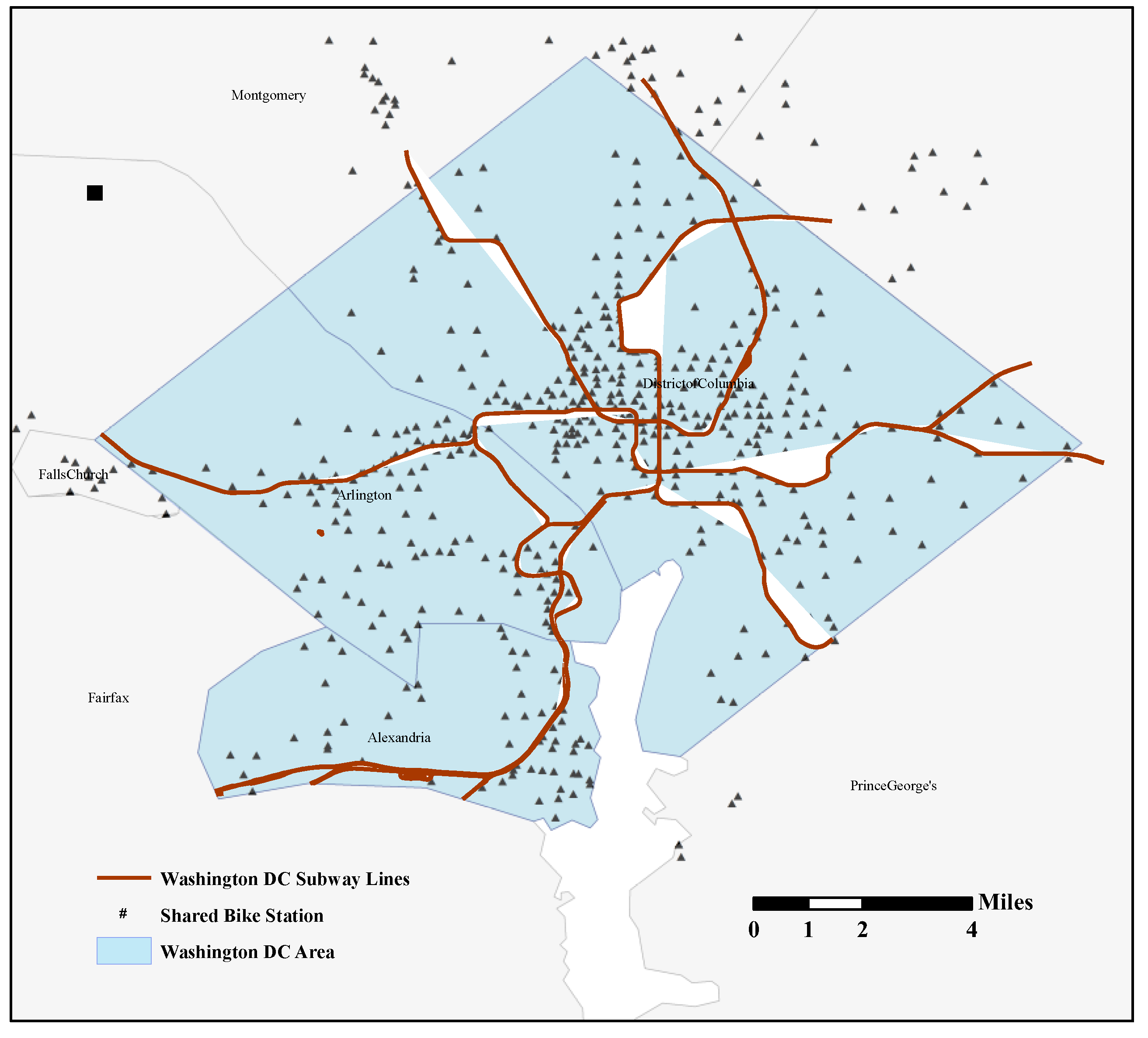
Figure 2.
Changes in the density of shared bike orders near subway stations, (a) Changes in the spatial density of shared bike stations near subway stations with different buffer radius, (b) Kernel density analysis of shared bike orders near McPherson Square subway station.
Figure 2.
Changes in the density of shared bike orders near subway stations, (a) Changes in the spatial density of shared bike stations near subway stations with different buffer radius, (b) Kernel density analysis of shared bike orders near McPherson Square subway station.
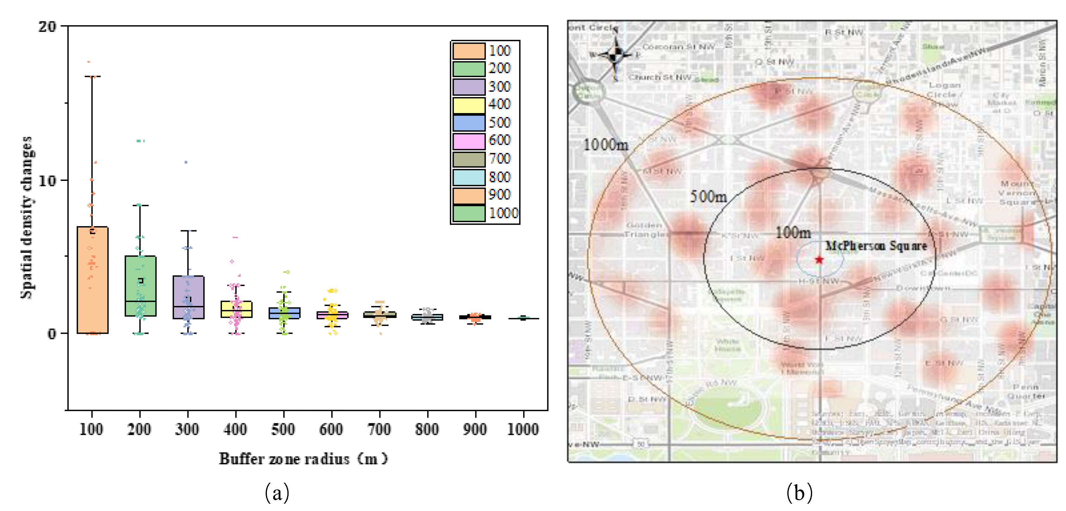
Figure 3.
Characteristics of spatial and temporal distribution of shared bike interchanges, (a) Annual trend of shared bike interchanges and total trips, (b) Hourly distribution of shared bike interchanges, (c) Hotspot distribution area of shared bike interchanges.
Figure 3.
Characteristics of spatial and temporal distribution of shared bike interchanges, (a) Annual trend of shared bike interchanges and total trips, (b) Hourly distribution of shared bike interchanges, (c) Hotspot distribution area of shared bike interchanges.
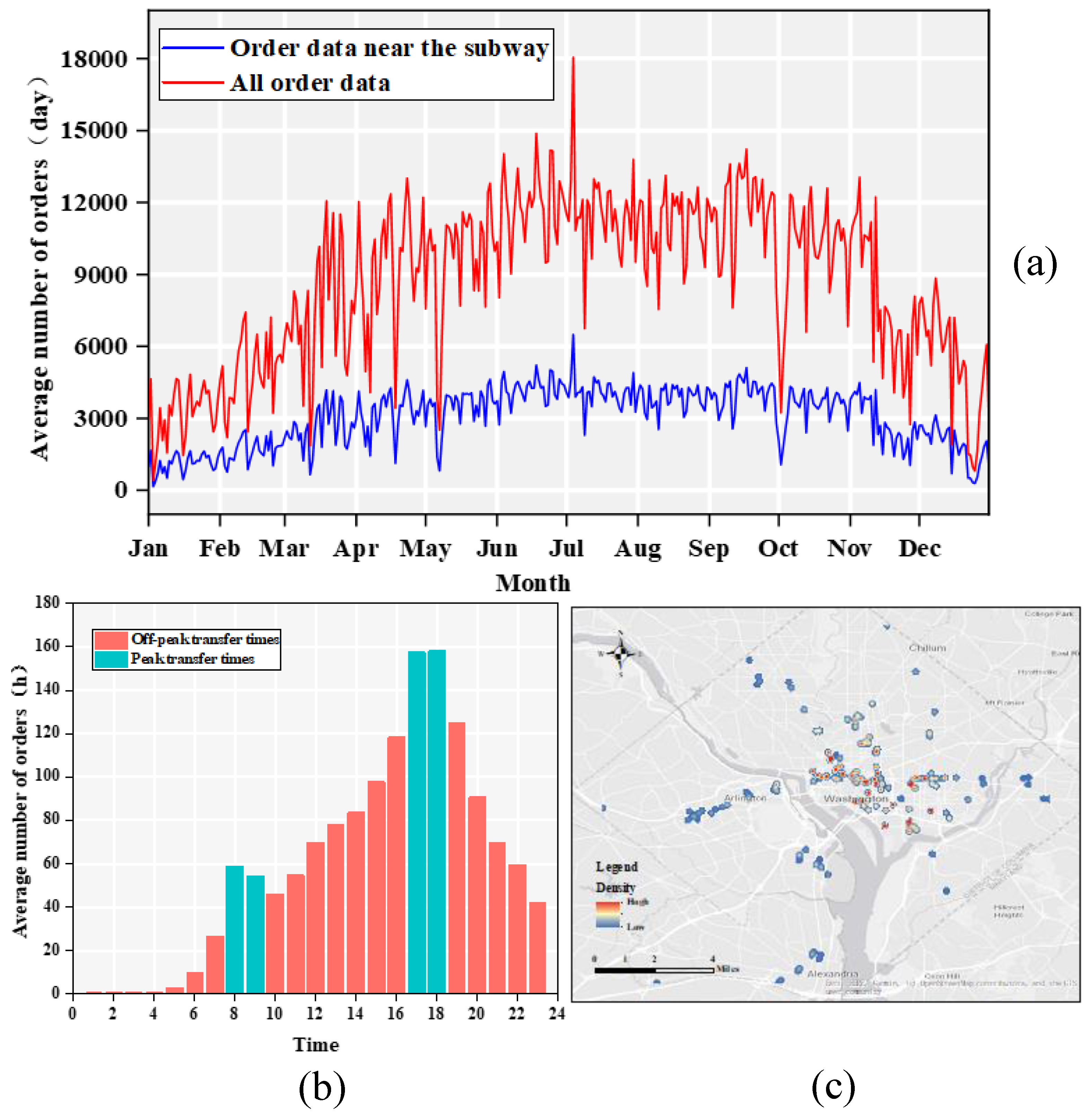
Figure 4.
Comparison plot of random forest model on training and test sets.
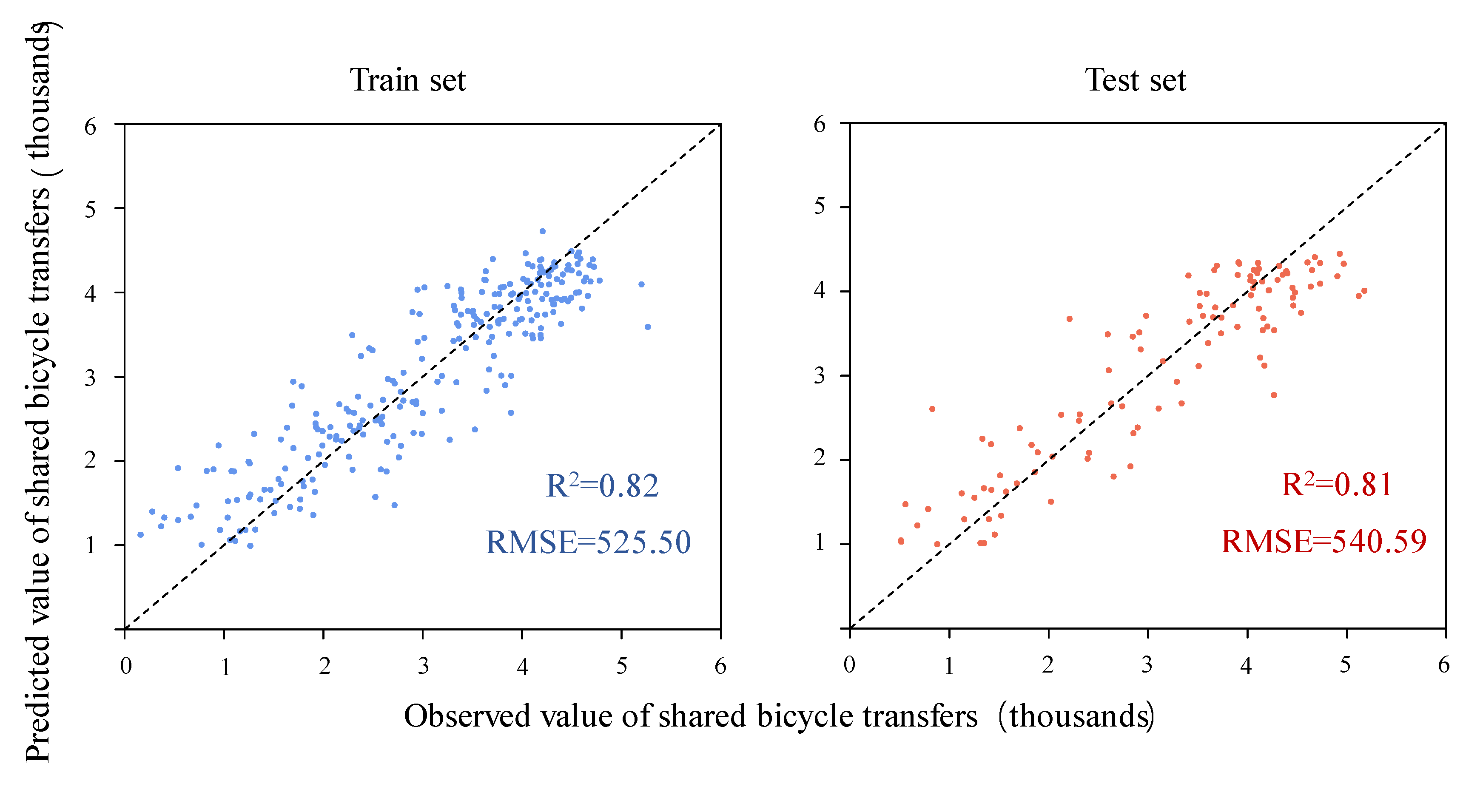
Figure 5.
Heatmap of global interaction effects with second-order interaction effect strengths for weather variables.
Figure 5.
Heatmap of global interaction effects with second-order interaction effect strengths for weather variables.
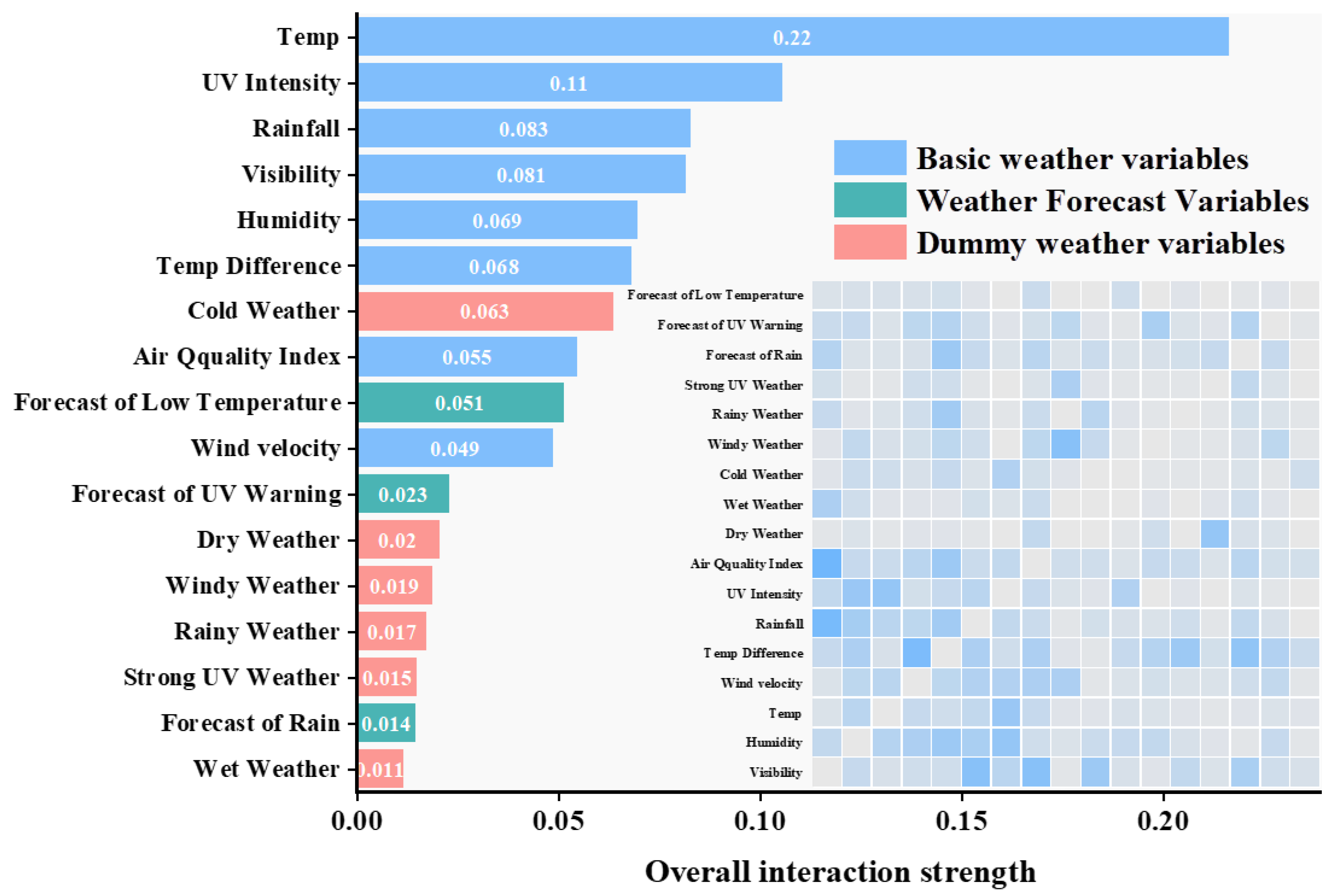
Figure 6.
Relative Importance Ranking of Weather Variables for Random Forest Models.
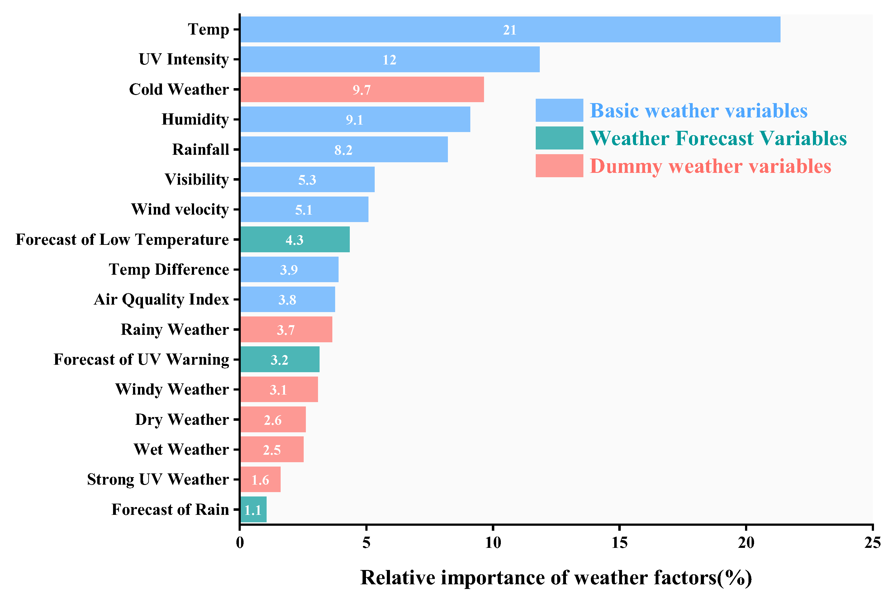
Figure 7.
presents the Accumulated Local Effects (ALE) plots for temperature and humidity: (a) Marginal effects plot of humidity on the bike-sharing transfer volume, (b) Marginal effects plot of temperature on the bike-sharing transfer volume, and (c) Second-order interaction effects plot between temperature and humidity.
Figure 7.
presents the Accumulated Local Effects (ALE) plots for temperature and humidity: (a) Marginal effects plot of humidity on the bike-sharing transfer volume, (b) Marginal effects plot of temperature on the bike-sharing transfer volume, and (c) Second-order interaction effects plot between temperature and humidity.
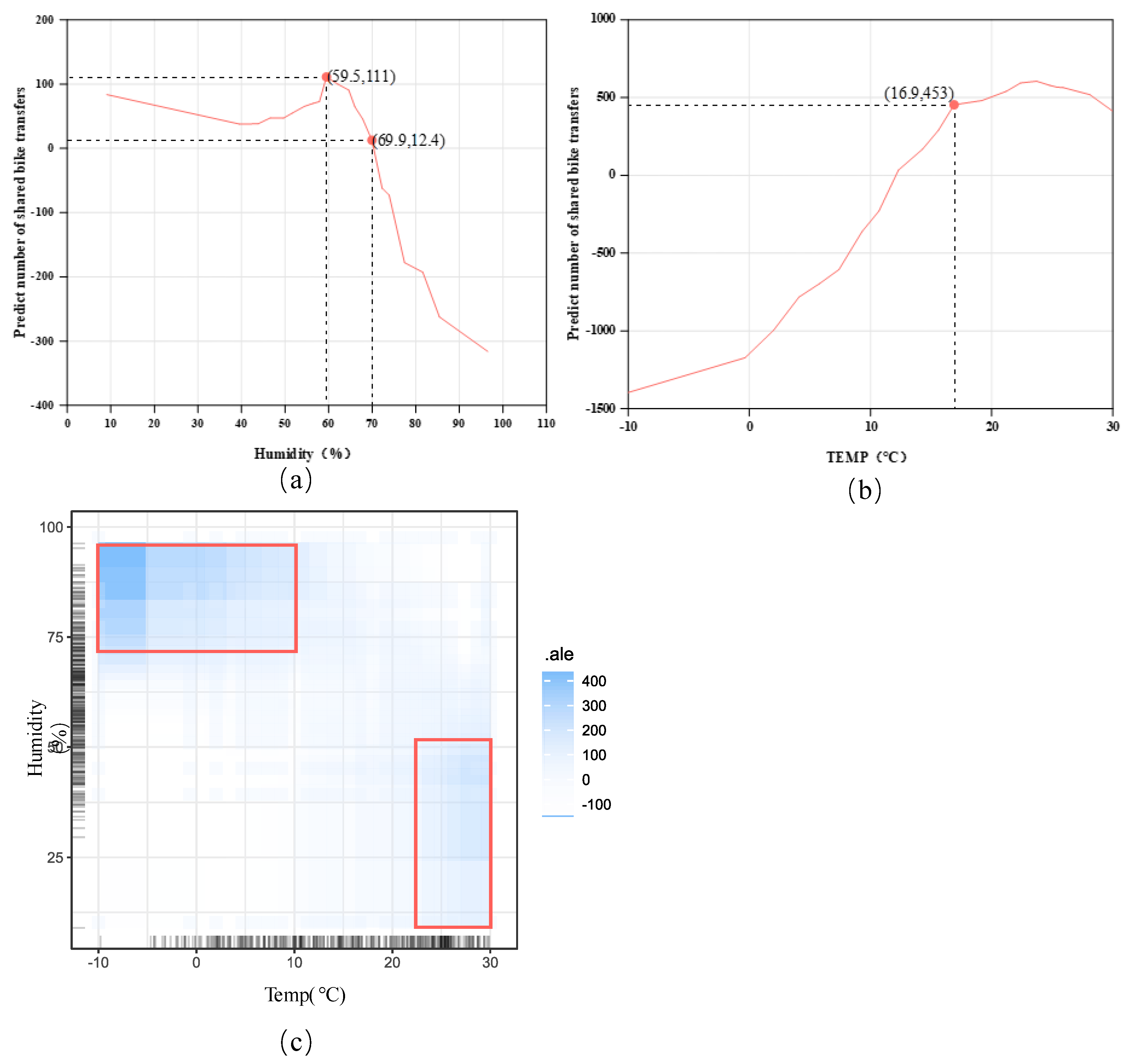
Figure 8.
Cumulative Partial Effects of Rainfall and Wind velocity(a) Marginal effects of rainfall on bike-sharing transfer volume(b) Marginal effects of wind speed on bike-sharing transfer volume(c) Second-order interaction effects between temperature and rainfall(d) Second-order interaction effects between temperature and wind velocity.
Figure 8.
Cumulative Partial Effects of Rainfall and Wind velocity(a) Marginal effects of rainfall on bike-sharing transfer volume(b) Marginal effects of wind speed on bike-sharing transfer volume(c) Second-order interaction effects between temperature and rainfall(d) Second-order interaction effects between temperature and wind velocity.
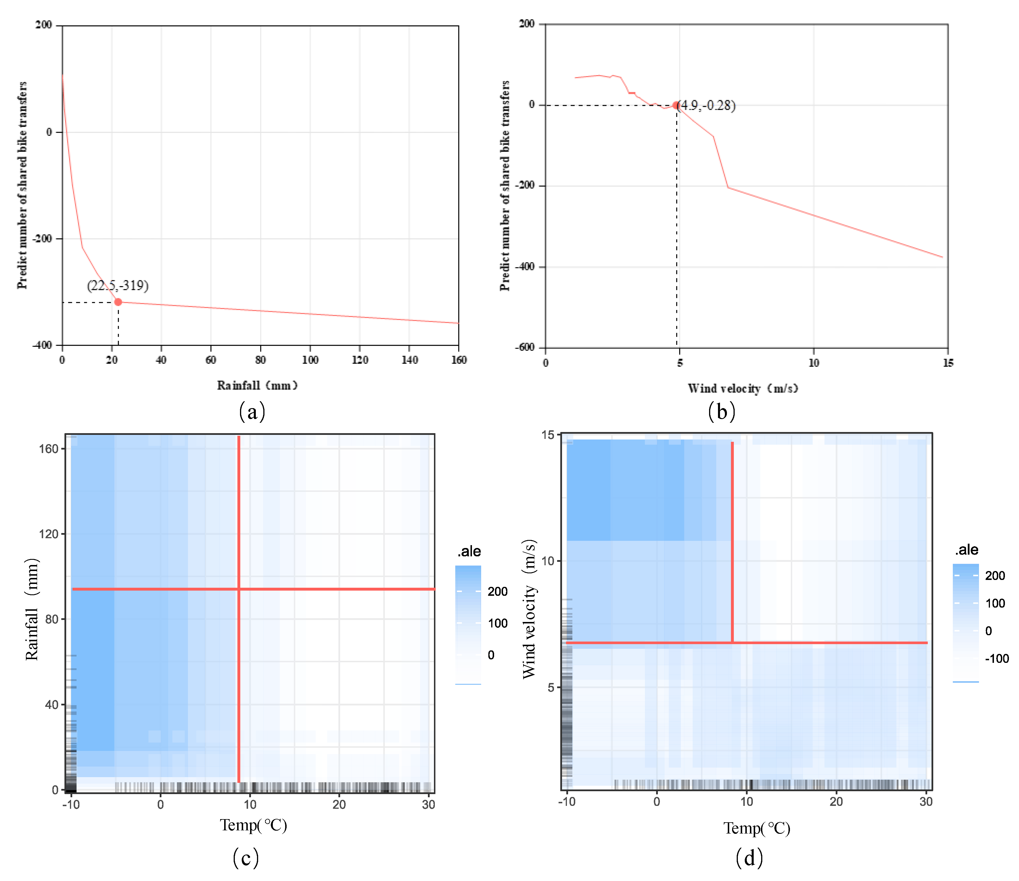
Figure 9.
shows the accumulated local effects of temperature difference and visibility. (a) depicts the marginal effect plot of temperature difference on the predicted bike-sharing transfer volume, while (b) illustrates the marginal effect plot of visibility on the predicted bike-sharing transfer volume.
Figure 9.
shows the accumulated local effects of temperature difference and visibility. (a) depicts the marginal effect plot of temperature difference on the predicted bike-sharing transfer volume, while (b) illustrates the marginal effect plot of visibility on the predicted bike-sharing transfer volume.
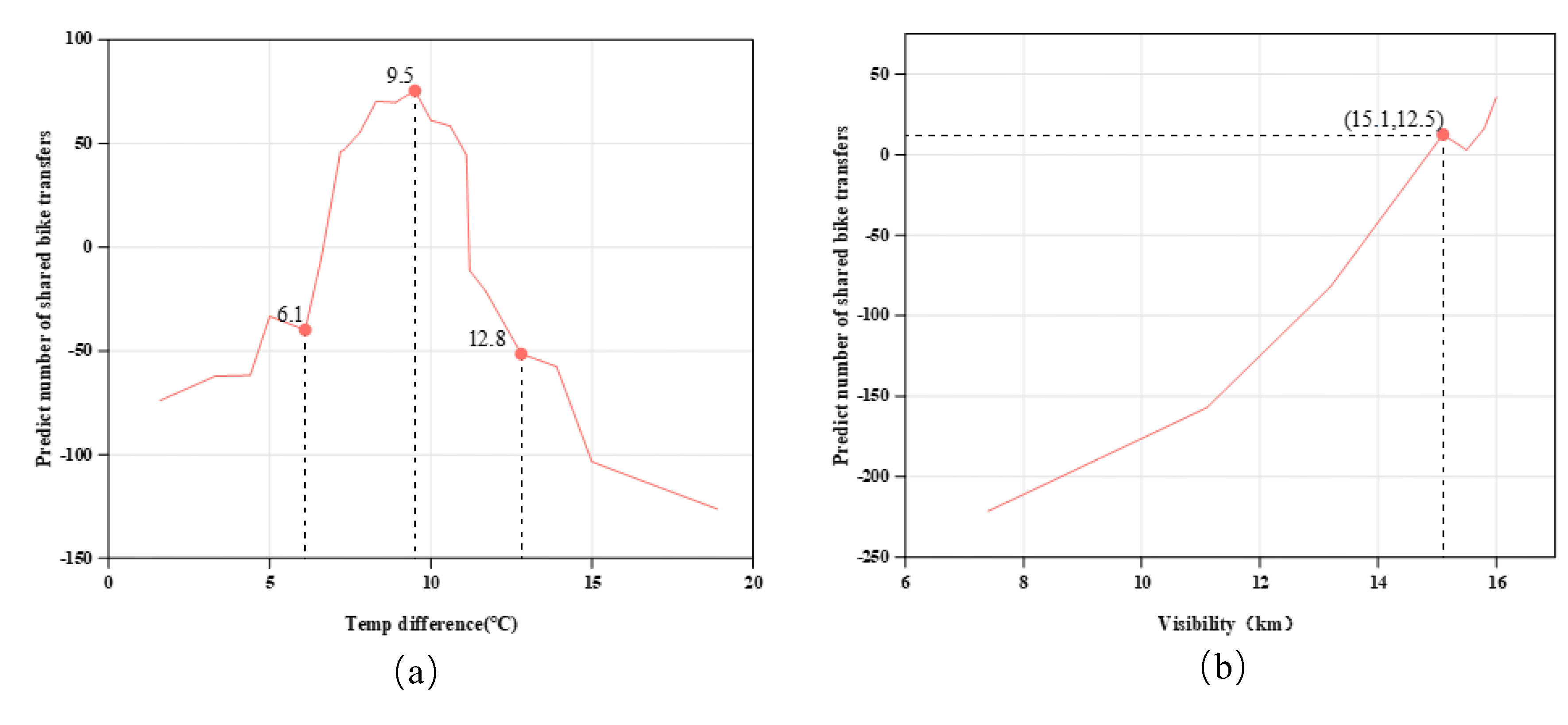
Figure 10.
presents the local cumulative effects of air quality. (a) displays the marginal effect plot of air quality on the predicted bike-sharing transfer volume. (b) and (c) show the second-order interaction effect plots between temperature and air quality, as well as humidity and air quality, respectively.
Figure 10.
presents the local cumulative effects of air quality. (a) displays the marginal effect plot of air quality on the predicted bike-sharing transfer volume. (b) and (c) show the second-order interaction effect plots between temperature and air quality, as well as humidity and air quality, respectively.
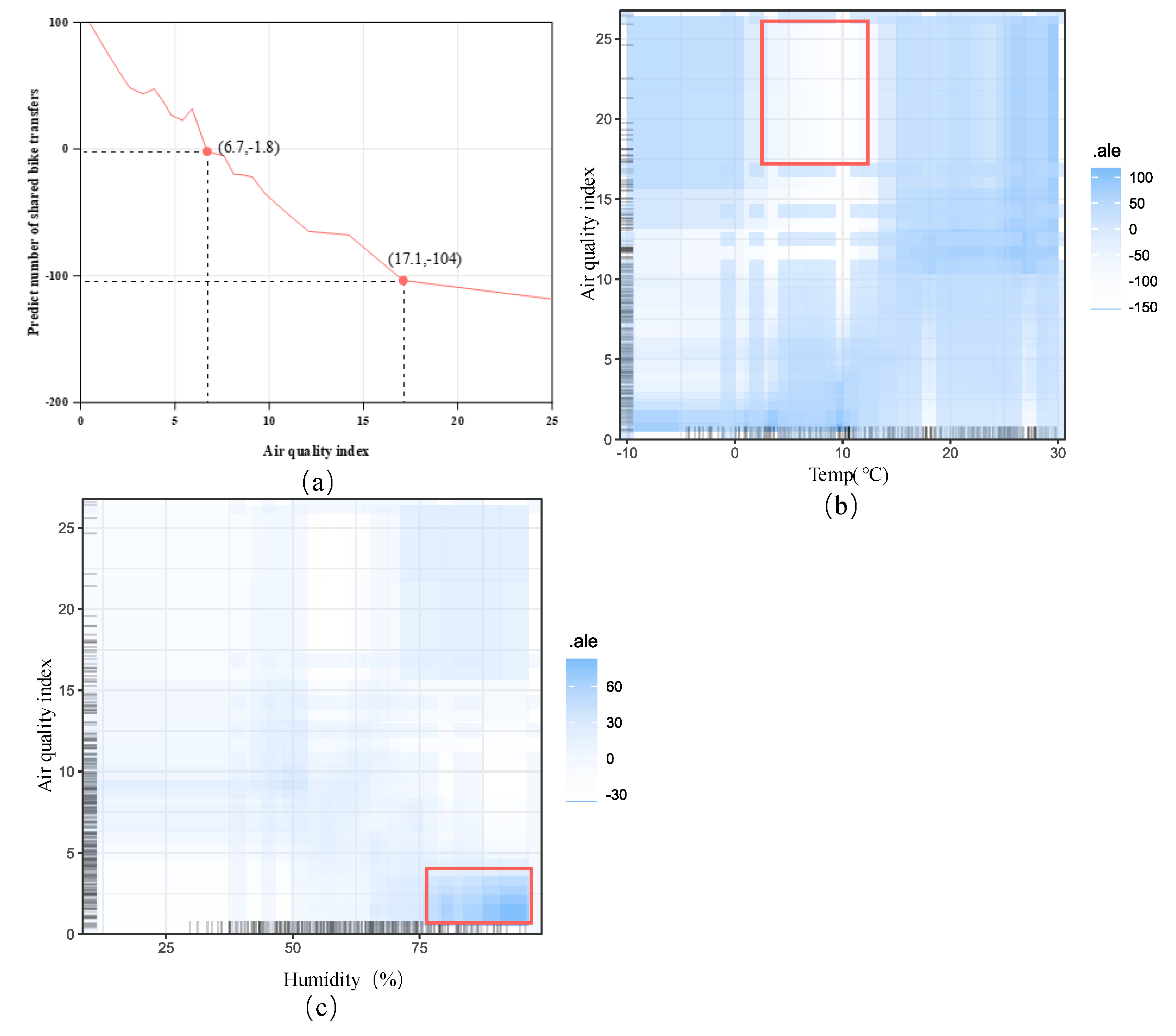

Table 1.
Data set source and description.
| Dataset | Source | Description |
|---|---|---|
| Air pollutant values | World Air Quality Index (WAQI) | Monitoring times, minimum value, maximum value, median, etc. |
| UV index | National Oceanic and Atmospheric Administration (NOAA) | The index range is 0-11 |
| Historical weather data | www.Rp5.ru | Temperature, visibility, humidity, wind speed, rainfall, etc. recorded every three hours |
| Map information data | OpenStreetMap (OSM) | City administrative region data, POI data, rail transit line network and site data |
| Shared bike order data | Capital bikeshare (CaBi) | User number, site name and its latitude and longitude, starting point and destination latitude and longitude, departure time and end time, user type and bike type, etc. |
Table 2.
Statistical description of weather independent variables.
| N | Min | Max | Average | SD | |
| Basic weather variables | |||||
| Visibility | 365 | 7.40 | 16.00 | 15.2759 | 1.62738 |
| Humidity | 365 | 9.10 | 96.50 | 62.0710 | 13.98713 |
| Temperature (Temp) | 365 | -10.00 | 30.01 | 15.0563 | 9.26532 |
| Wind velocity | 365 | 1.10 | 14.80 | 3.9992 | 1.53985 |
| Temp difference | 365 | 1.60 | 18.90 | 9.0345 | 3.54764 |
| Rainfall | 365 | .00 | 166.90 | 4.2077 | 12.53246 |
| UV intensity | 365 | .00 | 10.00 | 4.4521 | 2.85377 |
| Air quality | 365 | .50 | 26.40 | 7.5058 | 4.86157 |
| Dummy weather variable | |||||
| Wet weather | 365 | .00 | 1.00 | .1151 | .31954 |
| Dry weather | 365 | .00 | 1.00 | .1676 | .37401 |
| Cold weather | 365 | .00 | 1.00 | .1319 | .33881 |
| Wind weather | 365 | .00 | 1.00 | .1126 | .31658 |
| Rainy weather | 365 | .00 | 1.00 | .1374 | .34470 |
| Strong UV weather | 365 | .00 | 1.00 | .1154 | .31993 |
| Weather forecast variables | |||||
| Forest of rain | 365 | .00 | 1.00 | .2932 | .45583 |
| Forest of UV warning | 365 | .00 | 1.00 | .2060 | .40502 |
| Forest of low temp | 365 | .00 | 1.00 | .0549 | .22819 |
Table 3.
K-Means clustering results.
| Humidity | |||||
| Cluster center value | 41% | 54% | 65% | 74% | 85% |
| sample size | 63 | 103 | 89 | 68 | 42 |
| Temperature | |||||
| Cluster center value | 0 | 6 | 12 | 18 | 25 |
| sample size | 48 | 55 | 68 | 66 | 116 |
| Wind velocity | |||||
| Cluster center value | 1.7 | 2.6 | 3.5 | 4.8 | 6.9 |
| sample size | 23 | 63 | 114 | 87 | 41 |
| Rainfall | |||||
| Cluster center value | 0 | 2 | 16 | ||
| sample size | 242 | 72 | 51 | ||
| UV intensity | |||||
| Cluster center value | 1 | 2 | 3.5 | 7 | 9.1 |
| sample size | 37 | 69 | 83 | 92 | 42 |
| Ⅰ | Ⅱ | Ⅲ | Ⅳ | Ⅴ | |
Disclaimer/Publisher’s Note: The statements, opinions and data contained in all publications are solely those of the individual author(s) and contributor(s) and not of MDPI and/or the editor(s). MDPI and/or the editor(s) disclaim responsibility for any injury to people or property resulting from any ideas, methods, instructions or products referred to in the content. |
© 2025 by the authors. Licensee MDPI, Basel, Switzerland. This article is an open access article distributed under the terms and conditions of the Creative Commons Attribution (CC BY) license (http://creativecommons.org/licenses/by/4.0/).
Copyright: This open access article is published under a Creative Commons CC BY 4.0 license, which permit the free download, distribution, and reuse, provided that the author and preprint are cited in any reuse.