Submitted:
07 August 2025
Posted:
11 August 2025
You are already at the latest version
Abstract
The inspection of a series of lots from the same producer is a natural field of application of Bayesian approaches. On the one hand, it makes sense to take the posterior of the previous inspection as the prior of the next inspection. On the other hand, such a naive approach can quickly lead to the situation where the prior represents so much accumulated information that new test results from the current lot inspection will hardly have any effect at all on the posterior and, hence, on the calculations of conformance probability, specific consumer risk or expected utility. In other words, a naïve serial implementation of a Bayesian approach could result in such a level of information saturation that any further lot inspection would be meaningless. In effect, such a situation would be similar to having, e.g., complete trust in the producer and accepting all lots on faith. For this reason, it is important to carefully consider exactly how the conformance probability or the utility approach is applied in practice. The present paper describes a fully developed procedure for implementing these two approaches in connection with serial lot inspection. In this approach, a data-ageing procedure is described. The basic principle is to downweight older data in such way as to prevent information saturation in the sense of over-informative priors. Moreover, when the sample size, the expected value for the proportion nonconforming and the inspection frequency are constant, it is possible to derive closed expressions for the expected values of the hyperparameters. These, in turn, allow a pragmatic approach for the specification of inspection frequency or sample size.
Keywords:
acceptance sampling
; serial lot inspection
; Bayesian statistics
; sample size
; sampling frequency
1. Introduction
An approach for designing acceptance sampling plans for the inspection by attributes of isolated lots on the basis of the concept of conformance probability was described in Uhlig et al. (2024) [1]. The calculations involve Bayesian prior and posterior distributions and this approach thus differs considerably from the classical approach described in the ISO 2859 series [4]. In the conformance probability approach, the focus is on risks, and several new definitions of risks are proposed (based in part on JCGM 106 [2]). This focus on risks is shared by the conformance probability and ISO approaches. By contrast, an approach centered on the concept of utility was described in Uhlig et al. (2025) [3]. In this approach, the plans are determined in order to maximize expected utility, which can be broadly defined as benefits minus costs. Both the conformance probability approach and the utility approach are Bayesian approaches to acceptance sampling.
The question naturally arises whether these Bayesian approaches can be implemented when lots from the same producer are inspected one after the other—i.e., in connection with the inspection of a series of lots. On the one hand, it makes sense to take the posterior of the previous inspection as the prior of the next inspection. On the other hand, such a naive approach can quickly lead to the situation where the prior represents so much accumulated information that new test results from the current lot inspection will hardly have any effect at all on the posterior and, hence, on the calculations of conformance probability, specific consumer risk or expected utility. In other words, a naïve serial implementation of a Bayesian approach could result in such a level of information saturation that any further lot inspection would be meaningless. In effect, such a situation would be similar to having, e.g., complete trust in the producer and accepting all lots on faith.
For this reason, it is important to carefully consider exactly how the conformance probability or the utility approach is applied in practice. The present paper describes a fully developed procedure for implementing these two approaches in connection with serial lot inspection.
It should be borne in mind that the procedures presented here are not suitable if the proportion nonconforming varies randomly from lot to lot.
2. Inspection of a Series of lots—Bayesian Updating Mechanism
At the core of Bayesian statistics lies the rule for combining prior information and testing outcomes to obtain a posterior distribution. This fusion of information from different sources constitutes the first aspect of the Bayesian updating mechanism. However, in the context of lot inspection, there is a second aspect: namely, taking the posterior from a previous inspection as the prior for the next inspection. The following notation is introduced in order to conveniently take both aspects into account. In connection with the inspection of a series of lots, the index denotes the current lot inspection and and denote the prior and posterior distributions in lot inspection , respectively. Similarly, denotes the testing outcome in lot inspection .
These two aspects are summarized in the Table 1.
A ‘naïve’ approach to serial lot inspection would consist in an iterative application of these two updating mechanisms, whereby the acceptance sampling plan for each inspection is determined via either the conformance probability (risk-based) approach, see Uhlig et al. (2024) [1] or the utility approach, see Uhlig et al. (2025) [3]. This is illustrated in the following Table 2, which shows acceptance sampling plans obtained by the conformance probability approach for two different scenarios corresponding to different initial priors. The threshold for the conformance region for proportion nonconforming is specified as = 10%. In scenario 1, the initial prior is Beta(1,9), while in scenario 2, the initial prior is Beta(1,19). Measured against the = 10% value, the initial prior for scenario 1 is quite conservative (bordering on pessimistic) while the initial prior for scenario 2 is more optimistic. The threshold for the specific consumer risk SCR() is specified as CRBayes = 5%. For both scenarios and for all inspections, it is assumed that testing outcomes are consistently . For each scenario, acceptance sampling plans for the first three inspections are provided.
As can be seen, for a given inspection , the same posterior—i.e., the same pair —is obtained for both scenarios. After 3 inspections, the posterior is Beta(1,31) for both scenarios and repeated application of the conformance probability approach may result in meaningless lot inspection insofar as testing outcomes for the current lot will have very little impact on the calculation of the posterior.
The following Table 3 shows acceptance sampling plans obtained via a ‘naïve’ serial application of the utility approach for the same two scenarios as in Table 2. For each scenario, the lot size is , the damages parameter is (which is )and the sampling & testing costs parameter is . Moreover, in both scenarios, we assume that testing outcomes are consistently .
3. Data Ageing and Half-Life: Higher Weighting of Recent Information, Lower Weighting of Old Information
As the number of inspections increases, the amount of information encoded in the prior will increase to the point where the posterior will hardly differ from the prior no matter the testing outcome. For this reason, in applying the conformance probability or utility approach in serial lot inspection, it is necessary to transform the posterior from the previous inspection before using it as the prior for the next inspection. This transformation should ensure that lot inspection remains meaningful in the sense that the posterior remains sensitive to the testing outcomes.
The most natural way to achieve this is to develop a procedure whereby information loses currency as time elapses. Such an approach has the considerable advantage of reflecting the common-sense notion that the results from a lot inspection which took place very recently can be considered a far more reliable indicator of lot quality than results from a lot inspection which took place some time ago. In other words: the proposed procedure is articulated around a weighting mechanism which is inversely proportional to the “age” of the data.
Information currency loss as a function of elapsed time can be expressed mathematically in terms of an information half-life time interval (in short: “half-life”), denoted . Suffice it to say here that the basic idea is to adjust the hyperparameters in such a way as to increase the variance of the estimate of the proportion nonconforming as time goes by. The degree to which the variance increases is controlled via the ratio . The increase in variance is taken as the mathematical equivalent of information losing value. The specific value of will depend on the context: the type of manufacturing process, the type of QC performed by the producer, the availability of QC data, the type of product, the property of interest, the frequency of lot inspection, etc. Nonetheless, it can be said that, in many scenarios, a sensible value for will lie somewhere between 6 and 12 months. The procedure for adjusting the hyperparameters in relation with will now be described.
3.1. Procedure
The hyperparameters are adjusted via multiplication with the factor where denotes the time interval between two consecutive lot inspections. If , then and the variance of the beta distribution corresponding to the adjusted hyperparameters is thus increased by a factor which—in the case of a Beta() prior—depends on the sum but tends to as increases, as shown in the Figure 1.
The procedure will now be described in detail. In the following, the beta distribution hyperparameter subscripts have the following meaning:
The same notation is used for .
Preliminary testing (prior to the first inspection)
tests are performed at time point , and nonconforming items are observed.
The preliminary estimate for the proportion nonconforming is thus .
First inspection
Hyperparameters for the prior distribution:
where denotes the factor reflecting the time elapsed between preliminary testing and the first inspection.
The acceptance sampling plan is determined e.g., via the conformance probability or utility approach, yielding the sample size . Accordingly, tests are performed at time point , and nonconforming items are observed.
Posterior distribution:
The estimate for the proportion nonconforming after the first inspection is
We also calculate the cumulative sample size as
We can thus rewrite the posterior hyperparameters as
Inspection
Hyperparameters for the prior distribution:
Where denotes the factor reflecting the time elapsed between inspection and inspection .
The acceptance sampling plan is determined e.g., via the conformance probability or utility approach, yielding the sample size . Accordingly, tests are performed at time point , and nonconforming items are observed.
Posterior distribution:
The estimate for the proportion nonconforming after inspection is .
We also calculate the cumulative sample size as
Via mathematical induction, the following closed expressions for the posterior hyperparameters after inspection are obtained:
where denotes the decrease in information currency between time point and time point
3.2. Example 1: Comparison of Three Scenarios with Constant Sample Size and Acceptance Number Specified in Advance
In order to illustrate how this approach affects the hyperparameters, we consider the simple case that 50%, corresponding to a Beta(1,1) prior (noninformative prior) and that for all inspections we have
where (time interval between consecutive inspections) remains the same from inspection to inspection.
Note: since sample size and acceptance number are specified in advance and held constant, this example can be considered to be ‘blind’ as to how the acceptance sampling plan is calculated (i.e., as to whether the conformance probability approach of the utility approach is applied.)
The following table provides an overview of 3 scenarios.

Table 4.
Overview of the three scenarios with for all 7 lot inspections.
| Scenario 1 | without taking data ageing into account |
| Scenario 2 | for = 350 days and = 50 days |
| Scenario 3 | for = 350 days and = 100 days |
The hyperparameters for 7 consecutive inspections are as follows.
Table 5.
Hyperparameters for three scenarios with constant (7 consecutive lot inspections per scenario).
Table 5.
Hyperparameters for three scenarios with constant (7 consecutive lot inspections per scenario).
| Scenario | Inspection | Prior | Posterior | ||
|---|---|---|---|---|---|
| Scenario 1 without taking data ageing into account |
1 | 1.00 | 1.00 | 1.00 | 11.00 |
| 2 | 1.00 | 11.00 | 1.00 | 21.00 | |
| 3 | 1.00 | 21.00 | 1.00 | 31.00 | |
| 4 | 1.00 | 31.00 | 1.00 | 41.00 | |
| 5 | 1.00 | 41.00 | 1.00 | 51.00 | |
| 6 | 1.00 | 51.00 | 1.00 | 61.00 | |
| 7 | 1.00 | 61.00 | 1.00 | 71.00 | |
| Scenario 2 for = 350 days and = 50 days |
1 | 0.87 | 0.87 | 0.87 | 10.87 |
| 2 | 0.75 | 9.42 | 0.75 | 19.42 | |
| 3 | 0.65 | 16.83 | 0.65 | 26.83 | |
| 4 | 0.56 | 23.26 | 0.56 | 33.26 | |
| 5 | 0.49 | 28.83 | 0.49 | 38.83 | |
| 6 | 0.42 | 33.66 | 0.42 | 43.66 | |
| 7 | 0.37 | 37.85 | 0.37 | 47.85 | |
| Scenario 3 for = 350 days and = 100 days |
1 | 0.75 | 0.75 | 0.75 | 10.75 |
| 2 | 0.56 | 8.08 | 0.56 | 18.08 | |
| 3 | 0.42 | 13.59 | 0.42 | 23.59 | |
| 4 | 0.32 | 17.72 | 0.32 | 27.72 | |
| 5 | 0.24 | 20.83 | 0.24 | 30.83 | |
| 6 | 0.18 | 23.17 | 0.18 | 33.17 | |
| 7 | 0.14 | 24.93 | 0.14 | 34.93 | |
Variances and mean values corresponding to the posterior hyperparameters after the seventh inspection for the three scenarios are as follows.
Table 6.
Variances and mean values corresponding to the hyperparameters after 7 inspections for the three scenarios.
Table 6.
Variances and mean values corresponding to the hyperparameters after 7 inspections for the three scenarios.
| SCENARIO | α | β | MEAN | VARIANCE | SD | RSD |
|---|---|---|---|---|---|---|
| SCENARIO 1 NO DATA AGEING |
1 | 71 | 1.39% | 0.00019 | 0.014 | 98.62% |
| SCENARIO 2 t = 50 |
0.37 | 47.85 | 0.76% | 0.00015 | 0.012 | 162.09% |
| SCENARIO 3 t = 50 |
0.14 | 34.93 | 0.39% | 0.00011 | 0.010 | 263.00% |
As can be seen, across several inspections the variance does not increase (as it does after multiplying the two beta distribution parameters by the same factor , see the discussion above). This is due to the fact that the mean value is not constant across inspections. However, the RSD does increase.
The following table shows the decrease in the sum of the two hyperparameters.
Table 7.
Sum of hyperparameters for the three scenarios.
| SCENARIO | SUM α71 + β71 |
|---|---|
| SCENARIO 1 NO DATA AGEING |
72 |
| SCENARIO 2 t = 50 |
48.22 |
| SCENARIO 3 t = 100 |
35.07 |
3.3. Example 2: Revisiting the Two Scenarios from
In this example, we revisit the two scenarios from Section 2 with = 350 days and = 175 days (i.e., ).
The following table shows the plans obtained via the half-life approach. Plans are calculated with the conformance probability approach. Note the reduction of from 32 (in Table 2) to slightly less than 12.
The following table shows the plans obtained via the half-life approach. Plans are calculated with the utility approach. Note the reduction of from 33 or 34 (in Table 3) to less than 13.
Table 8.
Half-life approach for serial lot inspection. Plans are calculated via the conformance probability approach with = 10% and CRBayes = 5%. In scenario 1, the initial prior is Beta(1,9) whereas, in scenario 2, the initial prior is Beta(1,19). It is assumed that testing outcomes are consistently . Compare with Table 2.
| Scenario | Inspection | ||||||
| 1 | 1 | 0.61 | 5.46 | 16 | 0 | 0.61 | 21.46 |
| 2 | 0.37 | 13.02 | 3 | 0 | 0.37 | 16.02 | |
| 3 | 0.22 | 9.71 | 2 | 0 | 0.22 | 11.71 | |
| 2 | 1 | 0.61 | 11.52 | 10 | 0 | 0.61 | 21.52 |
| 2 | 0.37 | 13.06 | 3 | 0 | 0.37 | 16.06 | |
| 3 | 0.22 | 9.74 | 2 | 0 | 0.22 | 11.74 |
Table 9.
Half-life approach for serial lot inspection via the utility approach for , and . It is assumed that testing outcomes are consistently . Compare with Table 3.
Table 9.
Half-life approach for serial lot inspection via the utility approach for , and . It is assumed that testing outcomes are consistently . Compare with Table 3.
| Scenario | Inspection | ||||||
|---|---|---|---|---|---|---|---|
| 1 | 1 | 0.61 | 5.46 | 14 | 1 | 0.61 | 19.46 |
| 2 | 0.37 | 11.80 | 4 | 0 | 0.37 | 15.80 | |
| 3 | 0.22 | 9.58 | 3 | 0 | 0.22 | 12.58 | |
| 2 | 1 | 0.61 | 11.52 | 8 | 1 | 0.61 | 19.52 |
| 2 | 0.37 | 11.84 | 4 | 0 | 0.37 | 15.84 | |
| 3 | 0.22 | 9.61 | 3 | 0 | 0.22 | 12.61 |
3.4. Closed Expressions for the Hyperparameters for Constant , and
The three scenarios from Section 2 show that a ‘naïve’ application of Bayesian approaches in serial lot inspection may lead to ever increasing values for , and hence meaningless inspection. The half-life approach allows the user to control the values of . Indeed, applying the half-life adjustment to the three scenarios from Section 2 allows the sum to be reduced from over 30 to around 12 or 13 (after 3 inspections). We now explain why this is the case and derive formulas which will prove useful in the choice of the half-life , of the time interval between consecutive inspections and of the initial sample size.
Assume that we have a constant sample size , a constant expected value for the proportion nonconforming and a constant time interval between consecutive lot inspections. In other words, for all inspections
The requirement that the sample size be constant does not constitute a departure from what will typically be observed in serial lot inspection. Indeed, a rigorous application of the half-life approach will typically lead to a steep reduction in sample size until a constant low value is reached. For example, continuing the = 350 days and = 175 days (i.e., ) Scenario 1 example from Table 8 (conformance probability approach) the following plans are obtained for the first 10 inspections.
Table 10.
Half-life approach for serial lot inspection. Plans are calculated via the conformance probability approach with = 10% and CRBayes = 5%. The initial prior is Beta(1,9). It is assumed that testing outcomes are consistently . This table continues the first three rows of Table 8.
Table 10.
Half-life approach for serial lot inspection. Plans are calculated via the conformance probability approach with = 10% and CRBayes = 5%. The initial prior is Beta(1,9). It is assumed that testing outcomes are consistently . This table continues the first three rows of Table 8.
| Inspection | ||||||
|---|---|---|---|---|---|---|
| 1 | 0.61 | 5.46 | 16 | 0 | 0.61 | 21.46 |
| 2 | 0.37 | 13.02 | 3 | 0 | 0.37 | 16.02 |
| 3 | 0.22 | 9.71 | 2 | 0 | 0.22 | 11.71 |
| 4 | 0.14 | 7.10 | 1 | 0 | 0.14 | 8.10 |
| 5 | 0.08 | 4.92 | 1 | 0 | 0.08 | 5.92 |
| 6 | 0.05 | 3.59 | 1 | 0 | 0.05 | 4.59 |
| 7 | 0.03 | 2.78 | 1 | 0 | 0.03 | 3.78 |
| 8 | 0.02 | 2.29 | 1 | 0 | 0.02 | 3.29 |
| 9 | 0.01 | 2.00 | 1 | 0 | 0.01 | 3.00 |
| 10 | 0.01 | 1.82 | 1 | 0 | 0.01 | 2.82 |
As can be seen, the sample size quickly drops to and remains there (as long as testing outcomes remain ).
Under the assumption of constant , and parameters, it is possible to derive1 the following closed expressions for the expected values of the posterior hyperparameters and .
For we obtain
This allows us to define the -adjusted2 sample size . The following table shows the relationship between , and the asymptotic hyperparameter expected values for the simple case and .
Table 11.
r-adjusted sample size and asymptotic hyperparameter expected values for four different values and for and
Table 11.
r-adjusted sample size and asymptotic hyperparameter expected values for four different values and for and
| [days] | [days] | ||||
|---|---|---|---|---|---|
| 50 | 350 | 0.87 | 7.51 | 0 | 7.51 |
| 100 | 350 | 0.75 | 4.02 | 0 | 4.02 |
| 175 | 350 | 0.61 | 2.54 | 0 | 2.54 |
| 350 | 350 | 0.37 | 1.58 | 0 | 1.58 |
As can be seen, for days the limit of the expected value of the parameter is 2.54. This is the value to which the parameters are converging in Table 10.
There are two obvious applications of Equations (1) and Equation (2): deriving the sampling frequency and deriving the sample size.
Deriving the sampling frequency
If the sample size for all inspections is specified in advance and if it is known in advance what value for the serial inspections should converge to (thus capping the level of accumulated information incapsulated in the prior), suitable values for can be derived. For example, say that it is deemed desirable for to converge to 12, that the half-life value should be about one year (i.e., the choice days is appropriate) and that a value for close to zero is expected (i.e., simplifies to ). For , will converge to 12.2 for the choice days.
Table 12.
r-adjusted sample size and limits for the expected value of the hyperparameters for , , and
Table 12.
r-adjusted sample size and limits for the expected value of the hyperparameters for , , and
| 30 | 350 | 0.92 | 12.17 | 0 | 12.17 |
Deriving the sample size
Conversely, if a desired limit for has been specified and the inspection frequency has been prescribed, then it is possible to derive a suitable sample size. Say the time interval between consecutive lot inspections has been specified as days and that should converge to 12, then the choice is appropriate. The following table provides the hyperparameters for such a serial sampling scheme—whereby the sample size values for the first 3 lot inspections are 12, 9 and 6, respectively, before reaching the desired sample size of (this is done in order to build in an initial check regarding ).
Table 13.
Serial sampling scheme with =350 days and =100 days. As can be seen, for the sample size , the posterior parameter tends to 12, as desired.
Table 13.
Serial sampling scheme with =350 days and =100 days. As can be seen, for the sample size , the posterior parameter tends to 12, as desired.
| Inspection | Prior | Posterior | |||
|---|---|---|---|---|---|
| 1 | 12 | 0.75 | 0.75 | 0.75 | 12.75 |
| 2 | 9 | 0.56 | 9.58 | 0.56 | 18.58 |
| 3 | 6 | 0.42 | 13.96 | 0.42 | 19.96 |
| 4 | 3 | 0.32 | 15.00 | 0.32 | 18.00 |
| 5 | 3 | 0.24 | 13.53 | 0.24 | 16.53 |
| (…) | |||||
| 19 | 3 | 0.00 | 9.15 | 0.00 | 12.15 |
| 20 | 3 | 0.00 | 9.13 | 0.00 | 12.13 |
| 21 | 3 | 0.00 | 9.12 | 0.00 | 12.12 |
| 22 | 3 | 0.00 | 9.11 | 0.00 | 12.11 |
| 23 | 3 | 0.00 | 9.10 | 0.00 | 12.10 |
Another possibility to derive the sample size is to start from a range considered acceptable for (say between 20 and 100), and then to calculate the equivalent range for . In order to simplify the calculation, we introduce the notation
= number of lot inspections per half-life =
We thus have
and it follows that
The following table provides an overview of sample size values for different values of .
Table 14.
Range for the sample size as a function of corresponding to the range 20-100 for the r-adjusted sample size
Table 14.
Range for the sample size as a function of corresponding to the range 20-100 for the r-adjusted sample size
|
) |
) |
||
|---|---|---|---|
| 1 | 0.63 | 13 | 63 |
| 2 | 0.39 | 8 | 39 |
| 3 | 0.28 | 6 | 28 |
| 4 | 0.22 | 4 | 22 |
| 5 | 0.18 | 4 | 18 |
| 6 | 0.15 | 3 | 15 |
| 7 | 0.13 | 3 | 13 |
| 8 | 0.12 | 2 | 12 |
| 9 | 0.11 | 2 | 11 |
| 10 | 0.10 | 2 | 10 |
| 11 | 0.09 | 2 | 9 |
| 12 | 0.08 | 2 | 8 |
As can be seen: if only one inspection is performed within a half-life period , the sample size should lie between and . However, if inspections are performed once a month, a sample size lying between and is sufficient.
4. Conclusions
In serial lot inspection, a naïve application of Bayesian methods in acceptance sampling can lead to the situation where the prior represents so much accumulated information that test results from the current lot inspection will hardly have any effect at all on the calculations of conformance probability, specific consumer risk or expected utility. In such a case, lot inspection would be meaningless. In addition, it is common sense that data loses currency as time goes by, and that more recent data should be given more weight than older data. For this reason, a procedure for serial Bayesian lot inspection is proposed with an appropriate weight function of time, where the time is standardized in terms of a reference half-life time interval.
This procedure can be used to ensure that current testing outcomes always have the desired degree of influence on the calculations. Moreover, when the sample size, the expected value for the proportion nonconforming and the inspection frequency are constant, it is possible to derive closed expressions for the expected values of the beta distribution hyperparameters. These, in turn, allow a pragmatic approach for the specification of inspection frequency or sample size.
More generally, the data ageing principle can be applied in many contexts where iterative Bayesian calculations are performed.
| 1 | Via the expression for the
|
| 2 | Recall that
|
References
- Uhlig S, Colson B, Kissling R, Ellis S, Hicks M, Vandenbemden J, Pennecchi F, Göb R, & Gowik P (2024) Acceptance Sampling Plans Based on Conformance Probability—Inspection of Lots and Processes by Attributes. Preprints. [CrossRef]
- JCGM 106:2012 Evaluation of measurement data – The role of measurement uncertainty in conformity assessment.
- Uhlig S, Colson B, Göb R, Pennecchi F, Ellis S, Hicks M, Vandenbemden J, Kissling R, & Gowik P (2025) Acceptance Sampling Plans Based on Utility Functions—Inspection of Lots and Processes by Attributes. Preprints. [CrossRef]
- ISO 2859-1:1999 Sampling procedures for inspection by attributes. Part 1: Sampling schemes indexed by acceptance quality limit (AQL) for lot-by-lot inspection.
- ISO 3951-1:2022 Sampling procedures for inspection by variables. Part 1: Specification for single sampling plans indexed by acceptance quality limit (AQL) for lot-by-lot inspection for a single quality characteristic and a single AQL.
- Brush G (1986) A comparison of classical and Bayes producer’s risk. Technometrics, February 1986, Vol. 28, No. 1.
- Chun Y H & Rinks D B (1998) Three Types of Producer’s and Consumer’s Risks in the Single Sampling Plan, Journal of Quality Technology, 30:3, 254-268. [CrossRef]
Figure 1.
Factor by which the variance of a beta distribution is increased by multiplying both hyperparameters by for the case , displayed as a function of the sum . Note: the factor by which the variance is increased tends to as .
Figure 1.
Factor by which the variance of a beta distribution is increased by multiplying both hyperparameters by for the case , displayed as a function of the sum . Note: the factor by which the variance is increased tends to as .
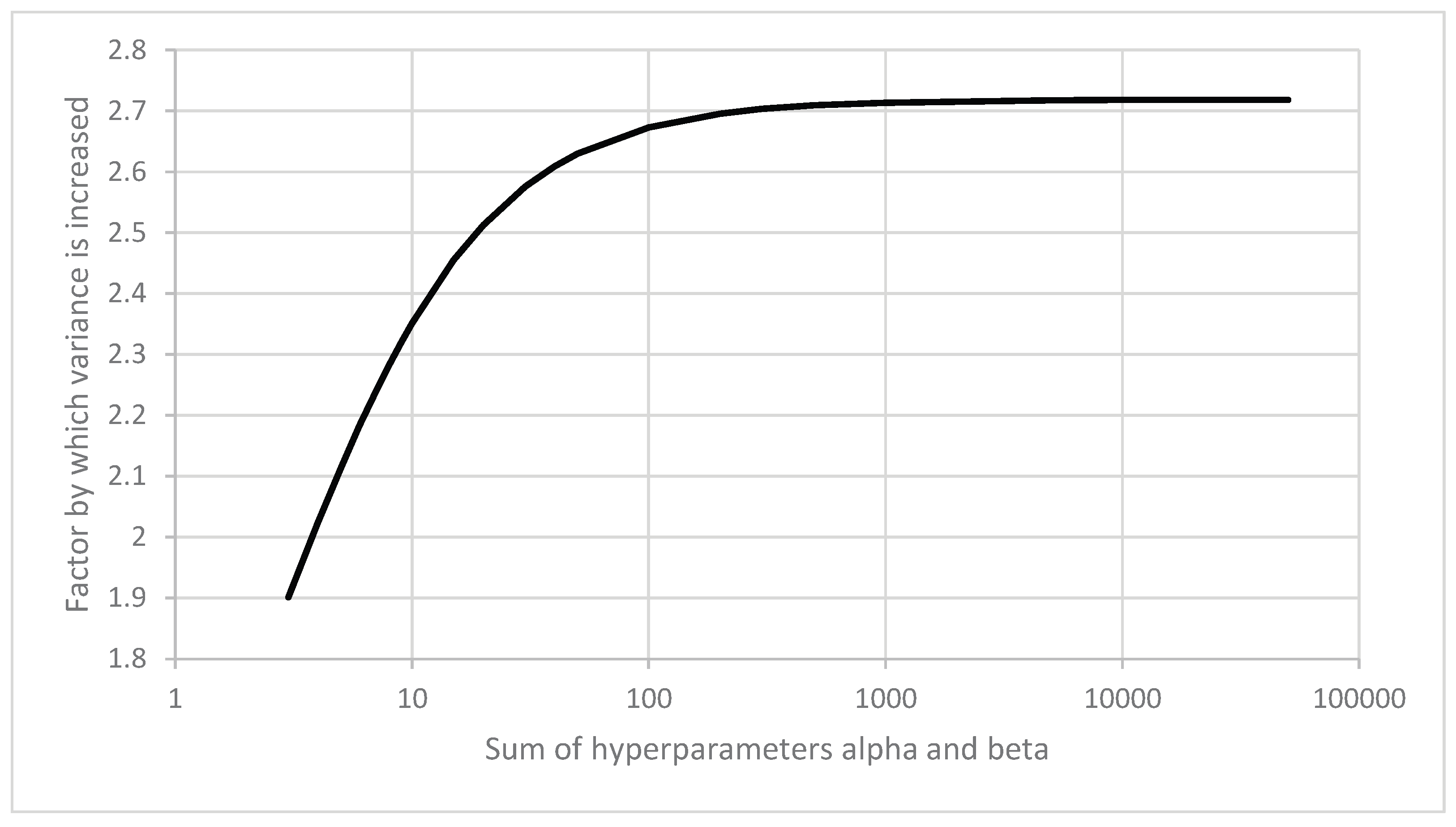
Table 1.
Two aspects of Bayesian updating in connection with the inspection of a series of lots.
| BAYESIAN UPDATING |
INSPECTION | INSPECTION |
|---|---|---|
| ASPECT 1 | The prior is updated to the posterior | |
| ASPECT 2 | The posterior is taken as the prior |
Table 2.
Naïve serial lot inspection via the conformance probability approach for = 10% and CRBayes = 5%. In scenario 1, the initial prior is Beta(1,9) whereas, in scenario 2, the initial prior is Beta(1,19). It is assumed that testing outcomes are consistently .
Table 2.
Naïve serial lot inspection via the conformance probability approach for = 10% and CRBayes = 5%. In scenario 1, the initial prior is Beta(1,9) whereas, in scenario 2, the initial prior is Beta(1,19). It is assumed that testing outcomes are consistently .
| Scenario | Inspection | ||||||
|---|---|---|---|---|---|---|---|
| 1 | 1 | 1 | 9 | 20 | 0 | 1 | 29 |
| 2 | 1 | 29 | 1 | 0 | 1 | 30 | |
| 3 | 1 | 30 | 1 | 0 | 1 | 31 | |
| 2 | 1 | 1 | 19 | 10 | 0 | 1 | 29 |
| 2 | 1 | 29 | 1 | 0 | 1 | 30 | |
| 3 | 1 | 30 | 1 | 0 | 1 | 31 |
Table 3.
Naïve serial lot inspection via the utility approach for , and . It is assumed that testing outcomes are consistently .
Table 3.
Naïve serial lot inspection via the utility approach for , and . It is assumed that testing outcomes are consistently .
| Scenario | Inspection | ||||||
|---|---|---|---|---|---|---|---|
| 1 | 1 | 1 | 9 | 15 | 1 | 1 | 24 |
| 2 | 1 | 24 | 4 | 0 | 1 | 28 | |
| 3 | 1 | 28 | 4 | 0 | 1 | 32 | |
| 2 | 1 | 1 | 19 | 7 | 1 | 1 | 26 |
| 2 | 1 | 26 | 4 | 0 | 1 | 30 | |
| 3 | 1 | 30 | 3 | 0 | 1 | 33 |
Disclaimer/Publisher’s Note: The statements, opinions and data contained in all publications are solely those of the individual author(s) and contributor(s) and not of MDPI and/or the editor(s). MDPI and/or the editor(s) disclaim responsibility for any injury to people or property resulting from any ideas, methods, instructions or products referred to in the content. |
© 2025 by the authors. Licensee MDPI, Basel, Switzerland. This article is an open access article distributed under the terms and conditions of the Creative Commons Attribution (CC BY) license (http://creativecommons.org/licenses/by/4.0/).
Copyright: This open access article is published under a Creative Commons CC BY 4.0 license, which permit the free download, distribution, and reuse, provided that the author and preprint are cited in any reuse.


