Submitted:
04 August 2025
Posted:
05 August 2025
You are already at the latest version
Abstract
Photoplethysmogram (PPG) signals are increasingly utilized in wearable and mobile healthcare applications due to their non-invasive nature and ease of use in measuring physiological parameters, such as heart rate, blood pressure, and oxygen saturation. Recent advancements have highlighted green-light photoplethysmogram (gPPG) as offering superior signal quality and accuracy compared to traditional red-light photoplethysmogram (rPPG). Given the deterministic chaotic nature of PPG signals' dynamics, nonlinear time series analysis has emerged as a powerful method for extracting health-related information not captured by conventional linear techniques. However, optimal data conditions, including appropriate sampling frequency and minimum required time series length for effective nonlinear analysis, remain insufficiently investigated. This study examines the impact of downsampling frequencies and reducing time series lengths on the accuracy of estimating dynamical characteristics from gPPG and rPPG signals. Results demonstrate that a sampling frequency of 200 Hz provides an optimal balance, maintaining robust correlations in dynamical indices while reducing computational load. Furthermore, analysis of varying time series lengths revealed that the dynamical properties stabilize sufficiently at around 170 seconds, achieving an error of less than 5%. A comparative analysis between gPPG and rPPG revealed no significant statistical differences, confirming their similar effectiveness in estimating dynamical properties under controlled conditions. These results enhance the reliability and applicability of PPG-based health monitoring technologies.
Keywords:
photoplethysmography
; nonlinear dynamics
; nonlinear time series analysis
; data reduction
; computational efficiency
; wearable devices
1. Introduction
In recent years, with the increasing use of wearable devices and mobile devices in healthcare, the number of devices measuring the photoplethysmogram (PPG) signal has been on the rise[1,2,3,4]. PPG is a biological signal used in clinical practice and health monitoring, representing the pulse waves. The signal acquisition mechanism involves measuring changes in blood vessel volume that happen when the heart pumps blood by shining light onto the skin and detecting fluctuations in the transmitted or reflected light. [4,5]. The measurement is noninvasive and easy to perform. In the past, red and near-infrared light were used for PPG; however, over the last two decades, green light has been attracting attention due to its higher accuracy in detecting changes in blood flow, lower susceptibility to noise, and suitability for measurement at various locations [6,7,8,9,10]. Green light PPG (gPPG) has been shown to be equally promising for various applications as red light PPG (rPPG) [7,10,11].
PPG data can be analyzed to obtain relevant cardiovascular information, such as heart rate, blood pressure, oxygen saturation, and vascular stiffness index [4,7,12]. It has also been demonstrated that heart rate variability (HRV) derived from PPG can replace HRV measured by electrocardiography (ECG) [13,14]. Typical ECG measurements involve multiple electrodes and cables, which can cause discomfort to the subject and are not suitable for use in locations where electrical interference may occur. PPG, in contrast, is very effective as it causes minimal discomfort and is easy to use anywhere. Many studies have shown that PPG can also be used for the early detection of cardiovascular diseases [15,16,17,18] and mental health assessment [19,20,21,22], and thus can be utilized for professional health management. Additionally, PPG measurements are cost-effective and straightforward to operate, highlighting their suitability for everyday health monitoring. Moreover, advances in technology have enhanced the accuracy and miniaturization of PPG sensors, enabling the collection of more health data during daily activities and supporting self-care.
PPG, which is nowadays measured in various conditions, has been well investigated in terms of extracting heart rate variability (HRV). However, since the cardiovascular and respiration dynamics [23,24], especially the dynamics of PPG [11,25,26] have been shown to be deterministic chaos, nonlinear time series analysis has been applied in previous studies to extract information on health status directly from PPG dynamics. It has become clear that nonlinear dynamic features can be applied as health indicators [11,25,26,27]. Deterministic chaos is a phenomenon in which a system follows deterministic laws but exhibits unpredictable behavior, demonstrating a strong dependence on initial conditions and aperiodicity [28,29]. This type of information-rich and complex dynamics allows for the analysis of biological data, such as PPG signals, to identify potential health states that traditional linear models cannot capture.
Nonlinear time series analysis of PPG data is performed on data reconstructed into a delay coordinate system to capture the nonlinear dynamics of the system [29,30]. The analysis is then performed using various methods, such as recurrence plots, Lyapunov exponents, and fractal dimension analysis [29]. Recurrence plots (RP) can be used to visualize and quantify nonlinear dynamic properties by performing recurrence quantification analysis (RQA) [31,32,33]. In PPG data, RQA was confirmed to provide robust and more sensitive results [34]. It has been used to improve the ability to estimate systolic and diastolic blood pressure [35], user authentication [36], stress assessment [21], discrimination between preterm and full-term newborns [34], and various other studies have validated it as a method for diagnosing health conditions (Table 1).
Many studies up to this point have shown the usefulness of applying nonlinear time series analysis to PPG data, but they have been used in analyses with various time series lengths, such as 2 seconds [37], 30 seconds [19], 100 seconds [38], 120 seconds [17], and 300 seconds [39]. In general, knowing the statistical properties of time series is a prerequisite for time series analysis, since infinitely long observation data can always reliably capture the statistical properties of the random variation of the target [29,40]. Therefore, a long time series length is also required in nonlinear time series analysis, and past studies have shown that RQA can usually be estimated more accurately with longer time series lengths [31,41]. However, in PPG, due to noise, movement artifacts, nonstationarity, and other effects, short time series are often used in the analysis [35,36]. Moreover, using shorter time series can significantly optimize the computation load when performing nonlinear time series analysis.
To address the problem of the appropriate PPG time series length choice, a previous study [38] investigated the impact of rPPG time series length on its dynamical properties evaluation by RQA. In [38], it was demonstrated that the RQA index converged as the time series length increased. However, while the approach was validated using numerical models, the comparison was made with 120 seconds as the standard reference for time series lengths that varied up to 120 seconds, which ensured error convergence to zero but was insufficient to determine a lower error limit. As seen in Table 1, considering the time series length used in various applied studies, the reference time series length in [42] was short and insufficient as an indicator for accurate estimation. Moreover, as the reference time series length in the previous study was short, an important problem of nonstationarity in PPG data was left undiscussed. Also, from the perspective of the PPG signal itself, the characteristic differences between various wavelengths of light sources, their effects on dynamic status evaluation, and the optimal time series length and sampling frequency for measurement and analysis remain open for discussion. In this study, to facilitate more advanced analysis using PPG with reduced data, we utilize gPPG and rPPG to investigate the impact of PPG data time series length and compare them across different sampling frequencies using RQA.
Therefore, the purpose of this study is to investigate the impact of data reduction methods on extracting dynamic characteristics from gPPG and rPPG data in two main aspects. The first is data down-sampling. In this study, comparisons are made between the common data sampling frequencies used in PPG devices: 400 Hz, 200 Hz, and 100 Hz. Second, data with varying time series length: compared to the previous study [42], a longer time series length is used as a standard for comparison. Thus, the reference value in this study is 300 seconds, which is used in many advanced PPG-related studies, as shown in Table 1. At the same time, this duration provides signal stationarity, as will be discussed in Section 2.4.
This study investigates the effects of these two points using gPPG and rPPG to clarify their differences in data requirements. It also aims to propose minimal suitable frequency and time series length settings for estimating PPG dynamic features through nonlinear time series analysis methods.
2. Data
2.1. Photoplethysmogram Signal
Traditionally, photoplethysmography measures pulse waves by irradiating a light source onto the skin of a fingertip, earlobe, arm, etc., causing the light to be partially absorbed by the body’s tissues and detecting fluctuations in transmitted or reflected light. The PPG waveform formation mechanism is based on the fact that with each heartbeat, the blood volume in the vessels varies, affecting the rate of light absorption. The PPG recorded with transmitted light is called the transmission type and is measured using a fingertip or earlobe, through which light can pass. On the other hand, those that use reflected light are called reflection type and can be measured not only on the fingertips but also on the arms and other parts of the body. Near-infrared light (900 nm), red light (660 nm), and green light (530 nm) are commonly used as the light source [11]. When infrared or red light is used, its application is limited due to the influence of sunlight on infrared light. However, green light, which is less affected by external disturbances, has a high light absorption rate and is therefore suitable for outdoor use [57]. An illustration of each type of measurement method is shown in Figure 1.
The PPGs used in this study are the reflection type gPPG and the transmission type rPPG, which is similar to the rPPG signals used in [42]. The recording was performed using a green light (530nm) pulse wave sensor (Arduino [58]) with a sampling frequency of 500.0 Hz for gPPG, and a red (660 nm) and near-infrared (900nm) pulse wave sensor with a sampling frequency of 409.6 Hz (Tokyo Devices, Inc.) for rPPG.
2.2. Data Collection Experiment
The subjects of the experiment were 18 healthy male and female students from Tokyo City University, all in their 20s, with no history of heart disease. After explaining the purpose of the study, the experimental method, and the associated risks, all subjects were asked to sign a consent form and provide their consent to participate in the experiment. The experiment was conducted in a quiet room maintained at room temperature (24±1 ℃). Before the start of the experiment, the subjects’ blood pressure and heart rate were measured using a digital blood pressure monitor (Omron HCR-7106) to confirm that they were within normal limits (systolic blood pressure 90-129 mmHg and diastolic blood pressure less or equal than 80 mmHg [59]). After a short rest period, the resting state of each subject was measured for 10 minutes. If the measurements were not successful, they were repeated at a later time. The subjects were instructed to remain in a sitting position and to move as little as possible. As shown in Figure 2, rPPG was attached to the index finger of the right hand and gPPG to the middle finger. According to a previous study [5], differences in measurement position between these two fingers do not cause a significant difference in the PPG signal when recorded from healthy subjects.
2.3. Data Preprocessing
In this study, the sampling frequencies of the acquired PPG data are 500 Hz for gPPG and 409.6 Hz for rPPG. The PPGs are measured at various sampling frequencies, and 100-1000 Hz is used in the analysis [8,14,18,21,36]. Past studies have shown that 5 Hz is sufficient to calculate the average heart rate from PPG [60]. However, in analysis using the entire pulse waveform, the required sampling frequency is not clear, and various values are used as described above.
The PPG amplitude spectrum obtained by the Fourier transform, which represents the intensity of each frequency component of the signal, is shown in Figure 3. According to the sampling theorem, a sampling frequency of at least twice the highest frequency of the signal is required, and in particular, a sampling frequency of at least 10 times is sufficient to display and record waveforms [29] accurately.
For this reason, the frequencies compared in this study are 400 Hz to match the rPPG device with the highest sampling frequency, followed by 2x and 4x downsampling, i.e., 200 Hz and 100 Hz.
All PPG signals underwent preprocessing that involved removing trends first, followed by filtering with a fourth-order Butterworth filter [61,62] to eliminate noise and extract the pulse wave shape, as used in previous studies [8,42,48,62]. Figure 4 illustrates the filter’s frequency response. Figure 5 and Figure 6 display comparisons of raw and filtered PPG data for gPPG and rPPG, respectively.
2.4. Data Selection
2.4.1. Quality of PPG Data
When handling PPG, noise can easily be generated, which may negatively impact measurement accuracy and lead to incorrect results. Additionally, it is important to ensure that the quality of the PPG data obtained is maintained throughout the 10-minute measurement period in this study. Therefore, we evaluated the measured PPG data using skewness, which has been shown in a previous study to be an effective quality index [63,64]. Skewness () measures the symmetry (or lack of symmetry) of a probability distribution and is defined by Eq. (1).
where N is the number of data points in the signal, is the mean of the data, and σ is the standard deviation of the signal. This measure processes abnormal changes in noisy PPG signals [63], and a time series length of 5 seconds is sufficient for its calculation [64].
In this study, comparisons were made for 600 seconds of data, shifting them in a 5-second window, and data showing abnormal changes were judged as measurement failures. Figure 7 and Figure 8 show an example of a plot of the changes along with corresponding PPG time series, data sample shown in Figure 7 was recognized as normal, and Figure 8 demonstrates an example of a measurement failure.
2.4.2. Estimation of Stationarity Through Heart Rate
Another problem that arises when analyzing long PPG time series is the potential nonstationarity, such as changes in the subject’s state due to mental load during measurement, which raises a question of whether the PPG data obtained reflect a single state or not. To address this issue, we first perform HRV analysis. In general, when a person is under mental stress, the autonomic nervous system is affected [65]. HRV analysis is the most widely used and relatively efficient method for analyzing these changes. The waveform of PPG data consists of several peaks, similar to the electrocardiograms the highest peak is called the R wave, and the interval between the R wave and the next R wave is called the RR interval (RRI). Figure 9 shows a typical PPG waveform and Figure 10 shows the PPG waveform with the largest peaks plotted in red. The RRI is calculated by finding the interval between these red dots.
2.4.3. HRV Analysis
HRV analysis was conducted based on the extracted RRI data to verify whether the obtained PPG data were stationary during the data collection. HRV analysis includes time-domain indices and frequency-domain indices [65]. In this study, analysis is performed using both time-domain and frequency-domain indices.
In general, analysis methods using frequency-domain indices are challenging to handle because they cannot be used for short periods of time and require detailed parameter settings, as a measurement of five minutes or longer is standard [65]. On the other hand, analysis methods using time-domain indicators require relatively short measurement times and can be performed with simple calculations [65]. Therefore, the state of the subject is evaluated by calculating the frequency-domain index in a 5-minute window and the time-domain index in a window with an RRI of 120 points.
First, LF/HF is calculated from the power spectrum density as a frequency domain index. The power spectrum density can be calculated using the fast Fourier transform or the maximum entropy method, from which the low frequency component (LF) from 0.04 to 0.15 Hz and the high frequency component (HF) from 0.15 to 0.4 Hz can be calculated. The LF/HF is used as an index. In previous studies, LF/HF values of 0~2 are considered good, 2~5 are considered cautionary, and 5 or more are considered very cautionary as objective criteria for determining fatigue level [67,68]. Evaluation is based on the fluctuations of LF/HF, although individual differences may occur, such as in people with autonomic nervous system disorders.
Next, sd2/sd1 was obtained from the Poincaré plot as a time domain index. The Poincaré plot, also called the Lorenz plot, is constructed with the nth RRI on the horizontal axis and the n+1st RRI on the vertical axis. Figure 14 shows an example of a Poincaré plot. This is an example where the state is determined to have changed since 300 seconds. The standard deviation on the y=-x axis is sd1, the standard deviation on the y=x axis is sd2, and sd2/sd1 is used as a time domain index. This value has a high correlation with LF/HF and can be treated as an index for stress analysis [65]. Similar to LF/HF, evaluation is made based on the variation of this value. As an example, sd2/sd1 obtained from normal (stable) and unstable measurements are shown in Figure 15 and Figure 16
2.4.4. Results of PPG Data Selection
We assessed whether the subject’s state changed during the measurement using HRV analysis. Consequently, some subjects’ data were considered to have remained stable over the 10-minute experiment, while others showed significant changes during the recording. For the following analysis, only data in which the subject state did not change and that were identified to be of good quality were selected. Thus, in this study, data from 10 out of 18 subjects were used.
The duration of the experiment was set to 10 minutes, assuming the subjects could remain in a resting state for 10 minutes at the beginning of the experiment. However, it is clear that there are individual differences in the amount of time they can remain in a stable, i.e., stationary, resting state. Thus, for some of the data, such as shown in Figure 16, the resting state changed during the experiment. In these data, the state of the subject changed significantly after more than 300 seconds from the start of the experiment. Therefore, 300 seconds, which is the standard value used in this study as described above, may be viewed as the time a person can remain in a resting state in a sitting position, taking into account individual differences.
Therefore, from this HRV analysis, it can be inferred that 300 seconds is a good standard value for comparison when changing the length of the time series.
3. Analysis Methods
3.1. Reconstruction into a Delay Coordinate System
In many real-world observations, it is impossible to observe all state variables of a nonlinear dynamical system simultaneously; therefore, reconstruction to a delay coordinate system is used in nonlinear time series analysis to reproduce the original system from the obtained time series [29,69]. Reconstruction to a delay coordinate system is a method based on Takens’ embedding theorem to reproduce the multidimensional nature of the system and to reveal the hidden dynamical structure. Since it is generally believed that the entire state variables of the pulse wave system cannot be observed, and only one-dimensional data can be observed by PPG, reconstruction to a delay coordinate system was performed [11,25,26]. The reconstruction into a delay coordinate system transforms the observed n-point-long time series data x(t) into an m-dimensional vector v(t) according to Eq. (3).
where τ is the time delay value, m is the reconstruction dimension, and t = 1,2,3,...,n.
The time delay value is often determined by autocorrelation [29]. In general, if the time delay value is too small, the correlation will be extremely high; therefore, an appropriate setting is necessary. In this study, the value of autocorrelation is calculated, and the time when it first becomes less than 1-1/e is used [42].
Next, the reconstruction dimension is determined by the false neighborhood method [29]. This allows to find the dimension in which the percentage of points that were neighbors in the m-1-dimensional space and are no longer neighbors in the m-dimensional space is close to zero.
3.2. Recurrence Plot
Recurrence plot (RP) visualizes the distance relationship between points on the attractor and is used for detecting dynamical behavior of time series [31,32,33]. RP is a two-dimensional binary image with a length of the total number of points on the attractor, N, and a matrix is created by Eq. (4):
where is i,jth pixel on RP, ε is the threshold value, and i,j are 1,2,3,...,N. In this study, the threshold value is set at a value where the recurrence rate (RR) of the recurrence plot obtained by Eq. (5) is close to 10% [31]:
3.3. Recursive Quantification Analysis (RQA)
RQA can extract quantitative features in the RP, and while there are a variety of methods, in this study, we calculated four values that characterize the diagonal lines [31,33]. These indices are important for quantitatively evaluating the regularity and chaos of the system and are suitable for the analysis of the dynamics of time series, which is the objective of this study.
D(l) is the number of diagonal lines of length l defined by Eq. (6). The RQA will be performed based on this value.
The first RQA index is determinism (DET), which is the ratio of points forming a diagonal line, as defined by Eq. (7). When a time series is deterministic, the DET value tends to be close to 1 [31]. Determinism means that the system is not created randomly but is driven by some rule.
The second index is . The orbit instability, or exponential orbit divergence, of a chaotic time series can be defined as the inverse of the longest diagonal in the RP, , defined by Eq. (8). Short indicates complex dynamics with rapid divergence, while longer values tend to indicate periodic behavior [31]. It is also considered to be inversely proportional to the Lyapunov exponent [31].
The third index is L. The average prediction time of an attractor is estimated by the average length L of the diagonal line, which is calculated by Eq. (9) [31]. The average prediction time indicates how long the system is predictable, and a long L suggests that the system is regular.
3.4. Error
The relative error, , for each of the above four RQA values, S, is determined by Eq. (12) for a given time series length, l, and a reference time series length, T= 300 seconds, which choice is discussed in Section 2.4.4.
4. Results
4.1. PPG Time Series Subsets
The choice of time series starting point may affect the analysis results, therefore, in this study, to proceed with analysis, subsets were created by varying the length of the preprocessed data every 10 seconds from 10 seconds (more than 10 cycles) to~ 200 seconds, with the initial position of the data shifted every 30 seconds. A reference data set for 300 seconds was also created in the same way. These were created for rPPG, gPPG at each frequency. As an example of the PPG data obtained, Figure 17 shows 10 seconds of rPPG and gPPG at each investigated frequency for the same person after pretreatment. Inspection of the waveforms of the PPG data reveals that no significant information loss occurred as the sampling frequencies varied in this study. However, when comparing gPPG and rPPG, differences can be seen in the waveforms.
4.2. Parameter Settings
For each PPG time series, we set parameters, reconstruct the delay coordinate system, create RPs, and perform RQA. First, as parameter settings, we obtain the time delay value τ and the reconstruction dimension m required for reconstruction to the delay coordinate system. The results of the autocorrelation function calculation and the false neighborhood method are presented in Figure 18, Figure 19, Figure 20 and Figure 21. These figures summarize the outcomes for 10, 60, and 120 seconds at each sampling frequency.
First, in the autocorrelation graph, as the time series length increases, only a slight change can be seen. This applies to all data, each having its own specific value. The variation with sampling frequency indicates that when the frequency is halved or quartered, the autocorrelation decreases correspondingly by the same factors.
Next, when examining the false neighborhood method results with longer time series, the false neighborhood ratio dropped to zero as the dimension increased from 4 to 5 at 10 seconds, suggesting four dimensions are sufficient. At 60 and 120 seconds, increasing the dimensions from 5 to 6 also resulted in a zero error neighborhood ratio, indicating five dimensions are sufficient. This pattern persisted even when lowering the sampling frequency. The results were similar for gPPG and rPPG.
4.3. Reconstructed Attractor and RP
Using the parameters obtained above, the reconstruction to the delay coordinate system and RP calculation was performed. The threshold of the RP was determined based on the RR, as described above, and was approximately 0.1 times the maximum distance between the points of the reconstructed attractor.
Figure 22, Figure 23, Figure 24 and Figure 25 show examples of the reconstructed attractors and RPs using the same subject’s data. The reconstructed attractor was 5-dimensional as defined in Section 4.2, but for visualization purposes, up to four dimensions are used here, and colors indicate the values in the fourth dimension.
The reconstructed attractors show a complex but recurrent behavior. The reconstructed attractor makes it easier to see the dependence on the frequency differences, which could not be seen with the PPG data as it is. Comparing the attractors of gPPG and rPPG, the shapes of the attractors seem to be similar, but they do not behave exactly the same, indicating that there are differences due to the wavelength of light and noise effects from the measurement equipment. To detect and quantify these features in detail, RPs were created, and RQA was performed.
4.4. RQA
The RQA is used to quantify the dynamical characteristics from the RPs. Figure 26 and Figure 27 show the changes in the values of each RQA result for the same subject. The changes in DET, L, and ENTR become more stable as the length of the time series increases. The value of for gPPG and rPPG stopped changing and remained constant when the time series length became longer. The results of gPPG and rPPG are not the same, especially the values of saturates faster for the rPPG.
4.5. Effects of Down-Sampling
First, we compare the effect of down-sampling at each frequency. Figure 28 and Figure 29 show a box-and-whisker plot of the RQA index values for each frequency (400 Hz, 200 Hz, and 100 Hz). The results show that all the indices show a decreasing trend when the frequency is lowered. A closer look at the effect of decreasing frequency shows that DET shows an increase in the variability of values, ENTR shows an overall decrease while the variability of values remains the same, and L and show a decrease in the variability of values and a more coherent distribution. Comparing the results for gPPG and rPPG, we can see that they show similar distributions.
In this study, we ranked the indicators at each frequency and calculated correlation coefficients between the down-sampled results and the rankings. Spearman’s rank correlation test was used. The results showed that statistically significant rank correlations existed for all data. The correlation coefficients are shown in Table 2 and Table 3.
The correlation coefficients show that there is a strong correlation overall, and that the down-sampling did not change the relative relationship much. In particular, for L, ENTR, and DET, there was a fairly strong positive correlation for all frequency combinations. However, for both gPPG and rPPG, the correlation compared to 400 Hz at shows that the correlation is weaker than for the other indices. However, 200Hz and 100Hz show strong correlations, as do the other indices. This indicates that down-sampling must be approached carefully if the higher frequencies are accurate, but it is also possible that the 400 Hz setting includes too much information when generating the RPs, leading to values different from the original ones. Looking at the distribution of in Figure 28 and Figure 29, the data are too scattered to represent the same resting state. Therefore, the overall result was that the relative position did not change much after down-sampling, and that 200 Hz may be suitable, considering the change in the distribution of the data.
4.6. Difference Between gPPG and rPPG by RQA
In the previous section, the possibility that gPPG and rPPG have similar distributions was suggested based on the box-and-whisker diagram. In this section, a Wilcoxon signed rank test was additionally performed on the dataset with a correspondence for each subject. This is due to the fact that the Shapiro-Wilk test did not verify the normal distribution of each RQA index. The results are summarized in Table 4.
The results show that there are no significant differences except for L and at 100 Hz, indicating that there are basically no significant differences between the values obtained by RQA for gPPG and rPPG at 400 Hz and 200 Hz. However, since the data at 100 Hz showed significant differences in the two indices, down-sampling to 100 Hz should be avoided because some information would be lost and a difference would be generated in the data where originally was no difference between gPPG and rPPG. However, the results in 4.5 show that there is a strong correlation with the 200 Hz data, and therefore, if one does not pay attention to the difference between gPPG and rPPG, there should be no particular problem in handling the data.
Combined with the results of section 4.5, it can be inferred that a sampling frequency of 200 Hz is appropriate for handling different types of PPG, since it suppresses the variability of all RQA indices and does not produce significant differences between rPPG and gPPG.
4.7. Effects of Time Series Length
Next, the effect of time series length is evaluated. To account for the realistic situation when the reference value is unknown, first, all data were analyzed with time series lengths of 10 to 200 seconds, and the error was calculated between the results for variable time series lengths and the reference value taken in the same 10 to 200 seconds range. Figure 30, Figure 31 and Figure 32 show a color map of the errors for 400 Hz, 200 Hz, and 100 Hz, respectively. The horizontal axis represents the time series lengths that were varied, and the vertical axis represents the time series lengths that were compared. For clarity, only the error values from 0.1 to 0 (10% to 0%) are color-coded.
The results show that the error for DET is almost zero in all cases and remains largely unaffected by the length of the time series. In contrast, the error for ENTR is generally low but increases slightly as the length of the compared time series grows. L exhibits a higher error than the previous two, and this error escalates as either the length of the time series or the reference time series increases, shown by the green and yellow areas. The rPPG results feature fewer yellow areas, although the impact of frequency is less noticeable. For both gPPG and rPPG, the error is very high and increases even when the time series length differs by 50 seconds from the length being compared. Across all results, the region of lower error, marked by the purple area, expands as the length of the investigated and reference time series increases. As the frequency decreases, the high-error area (represented by yellow) shrinks, and the error drops. While gPPG and rPPG results are quite similar, the 400 Hz data show that rPPG has slightly smaller yellow areas.
4.8. Error for gPPG with the Standard Reference Value (300 Seconds)
From this point on, the error from the reference value (300 seconds) is calculated for all data and compared with the time series length. First, the gPPG results are shown in Figure 33, Figure 34 and Figure 35 and Table 5. The results show that as the length of the time series increases, the error rate tends to decrease for all of the RQA indices. In terms of the degree of decrease, the error rates for DET and ENTR are quite low even at short time series lengths, and then decrease gradually. L drops from about 15% to about 3%. has a high error rate at short time series lengths, but this rate decreases significantly as the time series length increases. This trend was also observed across different frequencies.
The average error rate for DET was less than 1% at 10 seconds, and the higher the frequency, the lower the error rate. The ENTR 5% cutoff was 180 seconds at 400 Hz, 170 seconds at 200 Hz, and 170 seconds at 100 Hz, and the lower the frequency, the lower the cutoff. The 5% cutoff was not reached at 400 Hz, but achieved at 200 Hz for 160 seconds and at 100 Hz for 150 seconds.
The standard deviations (σ) of the error rates for all RQA indices were smallest at 200 s. For the DET, ENTR, and L indices, standard deviations were large at short time series lengths and then decreased, while the it was small at short time series lengths, then increased, and finally significantly decreased reaching a minimal value. This trend was also observed for different frequencies. A closer look at the effect of frequency shows that DET and ENTR become smaller as the frequency increases, while L and become smaller as the frequency decreases.
The errors from the reference value (300 seconds) for all RQA indices were less than 10% for 180 seconds at 400 Hz, 120 seconds at 200 Hz, and 100 seconds at 100 Hz, and less than 5% for 170 seconds at 200 Hz, and 170 seconds at 100 Hz, respectively.
4.9. Error for rPPG with the Standard Reference Value (300 Seconds)
The results of rPPG are shown in Figure 36 and Table 6. The results show a similar trend to that of gPPG, with the difference being that the mean error rate and standard deviation of L were higher at shorter times and then decreased, while the mean error rate and standard deviation of the other RQA indices were similar. However, the mean error rate at 200 seconds was lower for rPPG for DET and , and lower for gPPG for ENTR and L. The standard deviation trends were similar.
The mean error rate for DET was less than 1% at 10 seconds, and the higher the frequency, the lower the error rate. The L below 10% was achieved at 40 seconds for 400 Hz, 40 seconds at 200 Hz, and 40 seconds at 100 Hz, and below 5% at 140 seconds for 400 Hz, 150 seconds for 200 Hz, and 130 seconds for 100 Hz. The results show that the 10% cutoff at 400 Hz, 200 Hz, and 100 Hz was 120 seconds, and the 5% cutoff was 170 seconds at 400 Hz and 200 Hz, and 180 seconds at 100 Hz, with lower frequencies having lower cutoffs.
The error rate from the standard value (300 seconds) is less than 10% for all the RQA indices: 120 seconds for 400 Hz, 200 Hz, and 100 Hz, and less than 5% for 170 seconds for 400 Hz and 200 Hz, and 180 seconds for 100 Hz.
Figure 36.
Change in the average error rate (± 0.5σ) of rPPG (400 Hz) from the standard reference value.
Figure 36.
Change in the average error rate (± 0.5σ) of rPPG (400 Hz) from the standard reference value.
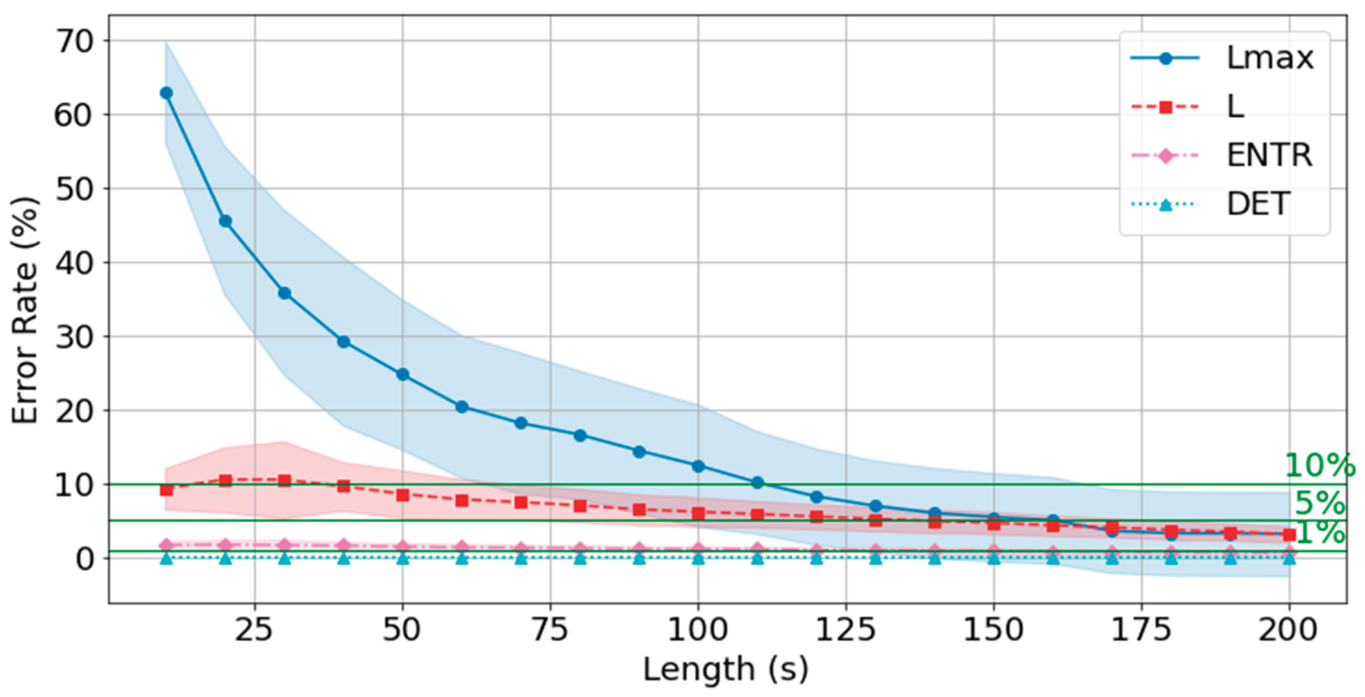
Figure 37.
Change in the average error rate (± 0.5σ) of rPPG (200 Hz) from the standard reference value.
Figure 37.
Change in the average error rate (± 0.5σ) of rPPG (200 Hz) from the standard reference value.
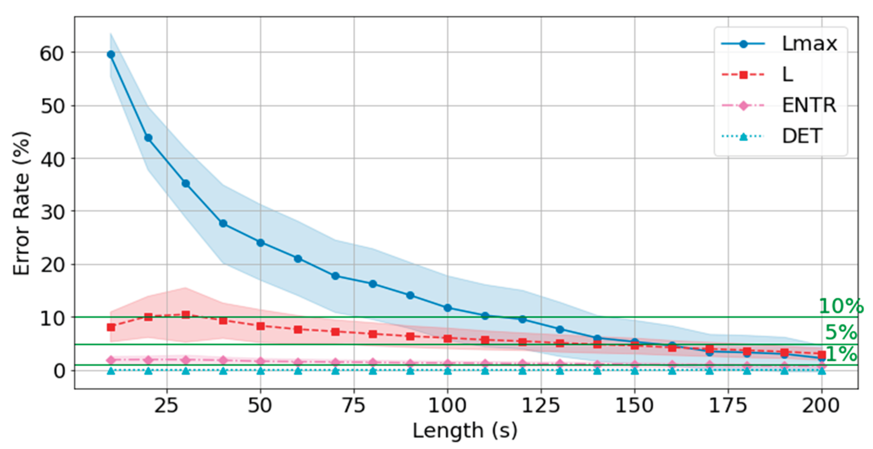
Figure 38.
Change in the average error rate (± 0.5σ) of rPPG (100 Hz) from the standard reference value.
Figure 38.
Change in the average error rate (± 0.5σ) of rPPG (100 Hz) from the standard reference value.
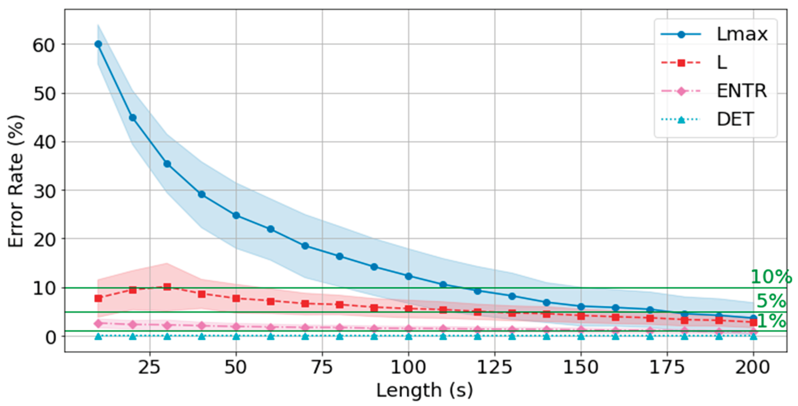

Table 6.
Summary of the average error rate (%) of rPPG RQA results compared with the reference value.
Table 6.
Summary of the average error rate (%) of rPPG RQA results compared with the reference value.
| time | 400Hz | 200Hz | 100Hz | |||||||||
| Lmax | L | ENTR | DET | Lmax | L | ENTR | DET | Lmax | L | ENTR | DET | |
| 10s | 62.898 | 9.272 | 1.638 | 0.002 | 59.245 | 8.432 | 1.950 | 0.009 | 59.447 | 7.916 | 2.651 | 0.062 |
| 20s | 45.576 | 10.500 | 1.698 | 0.001 | 44.217 | 10.231 | 2.009 | 0.007 | 44.910 | 9.541 | 2.380 | 0.049 |
| 30s | 35.891 | 10.498 | 1.640 | 0.001 | 35.843 | 10.497 | 2.001 | 0.007 | 35.216 | 10.084 | 2.319 | 0.053 |
| 40s | 29.250 | 9.613 | 1.571 | 0.001 | 27.330 | 9.433 | 1.860 | 0.007 | 28.858 | 8.717 | 2.115 | 0.052 |
| 50s | 24.730 | 8.569 | 1.438 | 0.001 | 23.973 | 8.475 | 1.688 | 0.006 | 24.623 | 7.822 | 1.984 | 0.047 |
| 60s | 20.420 | 7.817 | 1.329 | 0.001 | 21.131 | 7.783 | 1.607 | 0.006 | 22.021 | 7.318 | 1.890 | 0.044 |
| 70s | 18.147 | 7.454 | 1.297 | 0.001 | 17.512 | 7.355 | 1.538 | 0.006 | 18.259 | 6.709 | 1.775 | 0.043 |
| 80s | 16.584 | 7.015 | 1.225 | 0.001 | 15.899 | 6.958 | 1.467 | 0.005 | 15.986 | 6.567 | 1.761 | 0.041 |
| 90s | 14.427 | 6.470 | 1.137 | 0.001 | 13.932 | 6.526 | 1.382 | 0.005 | 14.020 | 6.053 | 1.626 | 0.039 |
| 100s | 12.437 | 6.158 | 1.125 | 0.001 | 11.744 | 6.258 | 1.368 | 0.005 | 11.855 | 5.791 | 1.584 | 0.038 |
| 110s | 10.135 | 5.842 | 1.079 | 0.001 | 10.421 | 5.926 | 1.309 | 0.005 | 10.236 | 5.624 | 1.555 | 0.035 |
| 120s | 8.228 | 5.511 | 1.009 | 0.000 | 9.748 | 5.662 | 1.242 | 0.004 | 9.083 | 5.265 | 1.460 | 0.033 |
| 130s | 6.952 | 5.186 | 0.975 | 0.000 | 8.094 | 5.323 | 1.205 | 0.004 | 8.046 | 4.943 | 1.399 | 0.032 |
| 140s | 5.982 | 4.914 | 0.942 | 0.000 | 6.549 | 5.003 | 1.157 | 0.004 | 6.850 | 4.740 | 1.367 | 0.030 |
| 150s | 5.434 | 4.658 | 0.873 | 0.000 | 5.888 | 4.765 | 1.074 | 0.003 | 6.099 | 4.361 | 1.252 | 0.027 |
| 160s | 5.024 | 4.308 | 0.817 | 0.000 | 5.238 | 4.399 | 1.012 | 0.003 | 5.803 | 4.082 | 1.178 | 0.026 |
| 170s | 3.562 | 4.033 | 0.772 | 0.000 | 4.138 | 4.129 | 0.963 | 0.003 | 5.468 | 3.858 | 1.137 | 0.024 |
| 180s | 3.257 | 3.707 | 0.714 | 0.000 | 3.931 | 3.862 | 0.900 | 0.003 | 4.644 | 3.494 | 1.035 | 0.022 |
| 190s | 3.233 | 3.455 | 0.668 | 0.000 | 3.544 | 3.554 | 0.825 | 0.002 | 3.975 | 3.290 | 0.950 | 0.020 |
| 200s | 3.203 | 3.111 | 0.609 | 0.000 | 2.454 | 3.170 | 0.754 | 0.002 | 3.433 | 2.912 | 0.858 | 0.019 |
5. Discussion
The purpose of this study was to investigate data reduction methods for PPG data that would minimize the amount of data used, sufficient, however, for extracting dynamical characteristics by methods of nonlinear time series analysis that were represented in this study by RQA. Although the effect of down-sampling could not be directly estimated from the waveforms of the PPG data, it was possible to visualize the effect of down-sampling and changing the length of the time-series by reconstructing the data into a delay coordinate system and creating RPs. Then RQA was performed to quantify RPs and compare the characteristics of the data.
First, the results of the down-sampling effect showed a decrease in the overall distribution of values for all RQA indices as the frequency decreased. However, for DET, the range of the distribution widened, and for L and , the distribution clumped together. Furthermore, a rank correlation check on whether the relative position of each value had changed revealed that correlations existed for all indicators. For the correlation was weaker compared with the L. The distribution of the data at 400 Hz was considerably wider than that of the others, suggesting that the data were scattered too much, even though they were from the same resting state, and thus may have contained excessive information in creating the RPs. From the changes in the overall distribution of the indices and the results of the rank correlation, it can be inferred that 200 Hz is an optimal and sufficient sampling frequency for PPGs.
Next, the effect of time series length was verified by comparing the results of 10 to 200 seconds with each other and with the standard value of 300 seconds. The results for the 10 to 200 second time series showed that DET had low errors for all time series lengths and was not affected by it. At the same time, ENTR had low errors as well and was not affected by the time series length. L, and tended to increase with distance from the compared time series length and to decrease with longer time series length, showing that the error was considerably affected by time series length. The results also showed that the error became lower as the frequency was lowered. For DET and ENTR, the errors were low starting at 10 seconds, and for L and the errors were high at shorter time-series lengths, and the errors decreased as the time-series length increased. When the frequency was lowered, DET and ENTR showed an increase in error, while L and showed a decrease in error. In the 200 Hz results, the error rate for all values is less than 5% at 170 seconds, and the standard deviation is not high, so we suggest using the 170-second data as sufficient time series length rather than the 300-second data. Although we have proposed an error rate of 5% here, the acceptable error rate can be more clearly suggested by checking the difference in each index using the RQA, for example, by comparing the results of a subject at rest and under stress, or by comparing the results of a patient with a certain disease.
Additionally, the comparison of these effects between gPPG and rPPG shows that there is no statistical difference in all the RQA indices, and the errors are not much different. It can be seen that there is no significant difference between the two measurement PPG setups.
6. Conclusions
Based on the above results, we propose the use of 200 Hz down-sampling and 170 s time series length for extracting dynamical information from PPGs by RQA in PPG if the state is constant. These results establish a basis for the data reduction, which is highly beneficial for various applications, such as health monitoring. At the same time, these results suggest the criteria for unifying the PPG data measurement requirements.
However, it is necessary to take into account that these results may change with a change in the subject state. Therefore, further validation in future work should include comparison with results at higher frequencies and validation of the extent to which the RQA index in PPG data changes under stress loads and other conditions.
Author Contributions
Conceptualization, N.S. and S.O.; methodology, N.S. and S.O.; software, S.O.; validation, N.S. and S.O.; formal analysis, N.S. and S.O.; investigation, N.S. and S.O.; resources, N.S.; data curation, N.S.; writing—original draft preparation, N.S. and S.O.; writing—review and editing, N.S.; visualization, S.O.; supervision, N.S.; project administration, N.S.; funding acquisition, N.S. All authors have read and agreed to the published version of the manuscript.
Funding
This research was partially supported by JST Moonshot R&D Grant Number JPMJMS2021.
Institutional Review Board Statement
The study was conducted in accordance with the Declaration of Helsinki, and approved by the Ethics Committee of Tokyo City University.
Informed Consent Statement
Informed consent was obtained from all subjects involved in the study.
Data Availability Statement
No data are available.
Conflicts of Interest
The authors declare no conflicts of interest.
Abbreviations
The following abbreviations are used in this manuscript:
| PPG | Photoplethysmogram |
| rPPG | Photoplethysmogram recorded with red light |
| gPPG | Photoplethysmogram recorded with green light |
| HRV | Heart Rate Variability |
| RP | Recurrence Plot |
| RQA | Recurrence Quantification Analysis |
References
- Park, J.; Seok, H.S.; Kim, S.-S.; Shin, H. Photoplethysmogram Analysis and Applications: An Integrative Review. Front. Physiol. 2022, 12. [Google Scholar] [CrossRef] [PubMed]
- Kim, K.B.; Baek, H.J. Photoplethysmography in Wearable Devices: A Comprehensive Review of Technological Advances, Current Challenges, and Future Directions. Electronics 2023, 12, 2923. [Google Scholar] [CrossRef]
- Namvari, M.; Lipoth, J.; Knight, S.; Jamali, A.A.; Hedayati, M.; Spiteri, R.J.; Syed-Abdul, S. Photoplethysmography Enabled Wearable Devices and Stress Detection: A Scoping Review. Journal of Personalized Medicine 2022, 12, 1792. [Google Scholar] [CrossRef] [PubMed]
- Photoplethysmography; Kyriacou, P.A., Allen, J., Eds.; 1st ed.; Academic Press: New Delhi, 2021; ISBN 978-0-12-823374-0.
- Allen, J. Photoplethysmography and Its Application in Clinical Physiological Measurement. Physiol. Meas. 2007, 28, R1–R39. [Google Scholar] [CrossRef]
- Maeda, Y.; Sekine, M.; Tamura, T.; Moriya, A.; Suzuki, T.; Kameyama, K. Comparison of Reflected Green Light and Infrared Photoplethysmography. Annu Int Conf IEEE Eng Med Biol Soc 2008, 2008, 2270–2272. [Google Scholar] [CrossRef]
- Tamura, T. Current Progress of Photoplethysmography and SPO2 for Health Monitoring. Biomed. Eng. Lett. 2019, 9, 21–36. [Google Scholar] [CrossRef]
- Lee, S.; Shin, H.; Hahm, C. Effective PPG Sensor Placement for Reflected Red and Green Light, and Infrared Wristband-Type Photoplethysmography. ICACT 2016, 556–558. [Google Scholar] [CrossRef]
- Maeda, Y.; Sekine, M.; Tamura, T. The Advantages of Wearable Green Reflected Photoplethysmography. J Med Syst 2011, 35, 829–834. [Google Scholar] [CrossRef]
- Tamura, T.; Maeda, Y.; Sekine, M.; Yoshida, M. Wearable Photoplethysmographic Sensors—Past and Present. Electronics 2014, 3, 282–302. [Google Scholar] [CrossRef]
- Sviridova, N.; Zhao, T.; Aihara, K.; Nakamura, K.; Nakano, A. Photoplethysmogram at Green Light: Where Does Chaos Arise From? Chaos, Solitons & Fractals 2018, 116, 157–165. [Google Scholar] [CrossRef]
- de Sá Ferreira, A.; Filho, J.B.; Cordovil, I.; de Souza, M.N. Three-Section Transmission-Line Arterial Model for Noninvasive Assessment of Vascular Remodeling in Primary Hypertension. Biomedical Signal Processing and Control 2009, 4, 2–6. [Google Scholar] [CrossRef]
- Chuang, C.-C.; Ye, J.-J.; Lin, W.-C.; Lee, K.-T.; Tai, Y.-T. Photoplethysmography Variability as an Alternative Approach to Obtain Heart Rate Variability Information in Chronic Pain Patient. J Clin Monit Comput 2015, 29, 801–806. [Google Scholar] [CrossRef] [PubMed]
- Gil, E.; Orini, M.; Bailón, R.; Vergara, J.M.; Mainardi, L.; Laguna, P. Photoplethysmography Pulse Rate Variability as a Surrogate Measurement of Heart Rate Variability during Non-Stationary Conditions. Physiol Meas 2010, 31, 1271–1290. [Google Scholar] [CrossRef] [PubMed]
- Fujita, D.; Suzuki, A.; Ryu, K. PPG-Based Systolic Blood Pressure Estimation Method Using PLS and Level-Crossing Feature. Applied Sciences 2019, 9, 304. [Google Scholar] [CrossRef]
- Rubins, U.; Grabovskis, A.; Grube, J.; Kukulis, I. Photoplethysmography Analysis of Artery Properties in Patients with Cardiovascular Diseases. 14th Nordic-Baltic Conference on Biomedical Engineering and Medical Physics 2008, 319–322. [CrossRef]
- Wright, G.; Caceres, J.L.H. Extracting Clinically Relevant Information from Pulse Oximetry Traces. Journal of Health Informatics in Africa 2017, 4. [Google Scholar] [CrossRef]
- Sharma, M.; Rajput, J.S.; Tan, R.S.; Acharya, U.R. Automated Detection of Hypertension Using Physiological Signals: A Review. International Journal of Environmental Research and Public Health 2021, 18, 5838. [Google Scholar] [CrossRef]
- Nakagome, K.; Makinodan, M.; Uratani, M.; Kato, M.; Ozaki, N.; Miyata, S.; Iwamoto, K.; Hashimoto, N.; Toyomaki, A.; Mishima, K.; et al. Feasibility of a Wrist-Worn Wearable Device for Estimating Mental Health Status in Patients with Mental Illness. Front Psychiatry 2023, 14, 1189765. [Google Scholar] [CrossRef]
- Wang, Z.-H.; Wu, Y.-C. A Novel Rapid Assessment of Mental Stress by Using PPG Signals Based on Deep Learning. IEEE Sensors Journal 2022, 22, 21232–21239. [Google Scholar] [CrossRef]
- Khaleghi, A.; Shahi, K.; Saidi, M.; Babaee, N.; Kaveh, R.; Mohammadian, A. Linear and Nonlinear Analysis of Multimodal Physiological Data for Affective Arousal Recognition. Cogn Neurodyn 2024, 18, 2277–2288. [Google Scholar] [CrossRef]
- Hu, Y.; Miyoshi, E. Technology development and the prospect of chaos analysis through pulse waves : The potential for the applied development of the correspondence method to mental illness in China. Bulletin of the Graduate School of Human Sciences, Osaka University 2014, 40, 27–46. [Google Scholar] [CrossRef]
- Small, M.; Judd, K.; Lowe, M.; Stick, S. Is Breathing in Infants Chaotic? Dimension Estimates for Respiratory Patterns during Quiet Sleep. Journal of Applied Physiology 1999, 86, 359–376. [Google Scholar] [CrossRef]
- Poon, C.-S.; Merrill, C.K. Decrease of Cardiac Chaos in Congestive Heart Failure. Nature 1997, 389, 492–495. [Google Scholar] [CrossRef] [PubMed]
- Sviridova, N.; Sakai, K. Human Photoplethysmogram: New Insight into Chaotic Characteristics. Chaos, Solitons & Fractals 2015, 77, 53–63. [Google Scholar] [CrossRef]
- Tsuda, I.; Tahara, T.; Iwanaga, H. Chaotic Pulsation in Human Capillary Vessels and Its Dependence on the Mental and Physical Conditions. Proceedings of the Annual Meeting of Biomedical Fuzzy Systems Association : BMFSA 1992, 4, 1–40. [Google Scholar] [CrossRef]
- Sumida, T.; Arimitu, Y.; Tahara, T.; Iwanaga, H. Mental Conditions Reflected by the Chaos of Pulsation in Capillary Vessels. Int. J. Bifurcation Chaos 2000, 10, 2245–2255. [Google Scholar] [CrossRef]
- Strogatz, S. Nonlinear Dynamics and Chaos: With Applications to Physics, Biology, Chemistry, and Engineering; 3rd ed.; CRC Press, 2014.
- Shelhamer, M. Nonlinear Dynamics in Physiology: A State-Space Approach; WORLD SCIENTIFIC, 2006; ISBN 978-981-270-029-2.
- Sviridova, N. Towards Understanding of Photoplethysmogram Dynamics through Nonlinear Time Series Analysis. SEISAN KENKYU 2019, 71, 141–145. [Google Scholar] [CrossRef]
- Marwan, N.; Carmen Romano, M.; Thiel, M.; Kurths, J. Recurrence Plots for the Analysis of Complex Systems. Physics Reports 2007, 438, 237–329. [Google Scholar] [CrossRef]
- Webber, C.L.; Zbilut, J.P. Dynamical Assessment of Physiological Systems and States Using Recurrence Plot Strategies. Journal of Applied Physiology 1994, 76, 965–973. [Google Scholar] [CrossRef] [PubMed]
- Recurrence Quantification Analysis: Theory and Best Practices; Webber, C.L., Marwan, N., Eds.; Understanding Complex Systems; Springer International Publishing: Cham, 2015; ISBN 978-3-319-07154-1.
- Skazkina, V.V.; Mureeva, E.N.; Ishbulatov, Y.M.; Prokhorov, M.D.; Karavaev, A.S.; Hramkov, A.N.; Ezhov, D.M.; Kurbako, A.V.; Panina, O.S.; Chernenkov, Y.V.; et al. Cross-Recurrence Quantification Of Cardiovascular Signals In Newborns Is A Sensitive Marker Of Health Status. Russ Open Med J 2024, 13, e0203. [Google Scholar] [CrossRef]
- Hamedani, N., Eslamyeh; Seyede, Z.S.; Mohammad, B.K. A CNN Model for Cuffless Blood Pressure Estimation from Nonlinear Characteristics of PPG Signals. ICBME 2021, 228–235. [Google Scholar] [CrossRef]
- Turkey, N.A.; Saleh, A.A.; Gaseb, A.; Ghaith, N.A. Recurrence Quantification Analysis for PPG/ECG-Based Subject Authentication | IEEE Conference Publication | IEEE Xplore. ICDIS 2022, 288–291. [Google Scholar] [CrossRef]
- Sviridova, N.; Ikeguchi, T. Application of Recurrence Quantification Analysis to Hypertension Photoplethysmograms. IEICE Proceedings Series 2020, 74. [Google Scholar]
- Khaleghi, A.; Shahi, K.; Saidi, M.; Babaee, N.; Kaveh, R.; Mohammadian, A. Linear and Nonlinear Analysis of Multimodal Physiological Data for Affective Arousal Recognition. Cogn Neurodyn 2024, 18, 2277–2288. [Google Scholar] [CrossRef] [PubMed]
- Mejía-Mejía, E.; May, J.M.; Elgendi, M.; Kyriacou, P.A. Classification of Blood Pressure in Critically Ill Patients Using Photoplethysmography and Machine Learning. Computer Methods and Programs in Biomedicine 2021, 208, 106222. [Google Scholar] [CrossRef] [PubMed]
- Ohtomo, N.; Terachi, S.; Tanaka, Y. Nonlinear Time Series Analysis : 1. A New Method of Analysis and the Theoretical Background. Nonlinear Time Series Analysis : 1. A New Method of Analysis and the Theoretical Background 1992, 158, 43–55. [Google Scholar]
- MARWAN, N. HOW TO AVOID POTENTIAL PITFALLS IN RECURRENCE PLOT BASED DATA ANALYSIS. International Journal of Bifurcation and Chaos 2011. [Google Scholar] [CrossRef]
- Sviridova, N.; Zhao, T.; Nakano, A.; Ikeguchi, T. Photoplethysmogram Recording Length: Defining Minimal Length Requirement from Dynamical Characteristics. Sensors 2022, 22, 5154. [Google Scholar] [CrossRef]
- Lu, H.; Yuan, G.; Zhang, J.; Liu, G. Recognition of Impulse of Love at First Sight Based On Photoplethysmography Signal. Sensors 2020, 20, 6572. [Google Scholar] [CrossRef]
- Chen, W.; Jiang, F.; Chen, X.; Feng, Y.; Miao, J.; Chen, S.; Jiao, C.; Chen, H. Photoplethysmography-Derived Approximate Entropy and Sample Entropy as Measures of Analgesia Depth during Propofol–Remifentanil Anesthesia. J Clin Monit Comput 2021, 35, 297–305. [Google Scholar] [CrossRef]
- Imanishi, A.; Oyama-Higa, M. On the Largest Lyapunov Exponents of Finger Plethysmogram and Heart Rate under Anxiety, Fear, and Relief States. 2007 IEEE International Conference on Systems, Man and Cybernetics 2007, 3119–3123. 3123. [CrossRef]
- Zhao, X.; Sun, G. A Multi-Class Automatic Sleep Staging Method Based on Photoplethysmography Signals. Entropy 2021, 23, 116. [Google Scholar] [CrossRef]
- Hina, A.; Saadeh, W. A 186μW Photoplethysmography-Based Noninvasive Glucose Sensing SoC. IEEE Sensors Journal 2022, 22, 14185–14195. [Google Scholar] [CrossRef]
- Goshvarpour, A.; Goshvarpour, A. Poincaré’s Section Analysis for PPG-Based Automatic Emotion Recognition. Chaos, Solitons & Fractals 2018, 114, 400–407. [Google Scholar] [CrossRef]
- Shi, P.; Xu, Y.; Guo, M.; Yu, H. Heart Rate Variability for Assessment of Fatigue of Central Motor Control in a Rhythmical Finger Tapping Task. CISP-BMEI 2017, 1–4. [CrossRef]
- Habbu, S.; Dale, M.; Ghongade, R. Estimation of Blood Glucose by Non-Invasive Method Using Photoplethysmography. Sādhanā 2019, 44, 135. [Google Scholar] [CrossRef]
- Li, N.; Yu, J.; Mao, X.; Zhao, Y.; Huang, L. The Nonlinearity Properties of Pulse Signal of Pregnancy in the Three Trimesters. Biomedical Signal Processing and Control 2023, 79, 104158. [Google Scholar] [CrossRef]
- Vraka, A.; Hornero, F.; Fácila, L.; Ravelli, F.; Alcaraz, R.; Rieta, J.J. Harnessing Photoplethysmography and Deep Learning in Continuous Blood Pressure Monitoring for Early Hypertension Detection. Advances in Digital Health and Medical Bioengineering 2024, 213–220. [Google Scholar] [CrossRef]
- Sviridova, N.; Sakai, K. Application of Photoplethysmogram for Detecting Physiological Effects of Tractor Noise. Engineering in Agriculture, Environment and Food 2015, 8, 313–317. [Google Scholar] [CrossRef]
- Miao, T.; Ogura, Y.; Fujita, E.; Oyama-Higa, M. Fluctuation Analysis of Finger Plethysmograms Related to Various Conditions. 2008 IEEE International Conference on Systems, Man and Cybernetics 2008, 3332–3337. 3337. [CrossRef]
- Xing, X.; Dong, W.-F.; Xiao, R.; Song, M.; Jiang, C. Analysis of the Chaotic Component of Photoplethysmography and Its Association with Hemodynamic Parameters. Entropy 2023, 25, 1582. [Google Scholar] [CrossRef]
- Wu, S.; Chen, M.; Wei, K.; Liu, G. Sleep Apnea Screening Based on Photoplethysmography Data from Wearable Bracelets Using an Information-Based Similarity Approach. Computer Methods and Programs in Biomedicine 2021, 211, 106442. [Google Scholar] [CrossRef] [PubMed]
- Pulse Sensor | Electronics Basics | ROHM. Available online: https://www.rohm.com/electronics-basics/sensors/sensor_what3 (accessed on 1 August 2025).
- Gitman, Y.; Murphy, J. Heartbeat Sensor Projects with PulseSensor: Prototyping Devices with Biofeedback; Apress: Berkeley, CA, 2023; ISBN 978-1-4842-9324-9. [Google Scholar]
- Carey, R.M.; Whelton, P.K. ; for the 2017 ACC/AHA Hypertension Guideline Writing Committee Prevention, Detection, Evaluation, and Management of High Blood Pressure in Adults: Synopsis of the 2017 American College of Cardiology/American Heart Association Hypertension Guideline. Ann Intern Med 2018, 168, 351–358. [Google Scholar] [CrossRef]
- Béres, S.; Hejjel, L. The Minimal Sampling Frequency of the Photoplethysmogram for Accurate Pulse Rate Variability Parameters in Healthy Volunteers. Biomedical Signal Processing and Control 2021, 68, 102589. [Google Scholar] [CrossRef]
- Scipy.Signal.Butter — SciPy v1.7.1 Manual. Available online: https://docs.scipy.org/doc//scipy-1.7.1/reference/reference/generated/scipy.signal.butter.html (accessed on 10 December 2024).
- Liang, Y.; Elgendi, M.; Chen, Z.; Ward, R. An Optimal Filter for Short Photoplethysmogram Signals. Sci Data 2018, 5, 180076. [Google Scholar] [CrossRef] [PubMed]
- Krishnan, R.; Natarajan, B.; Warren, S. Two-Stage Approach for Detection and Reduction of Motion Artifacts in Photoplethysmographic Data. IEEE Transactions on Biomedical Engineering 2010, 57, 1867–1876. [Google Scholar] [CrossRef] [PubMed]
- Elgendi, M. Optimal Signal Quality Index for Photoplethysmogram Signals. Bioengineering 2016, 3, 21. [Google Scholar] [CrossRef]
- Matsumoto, Y.; Mori, N.; Mitajiri, R.; Jiang, Z. Study of Mental Stress Evaluation based on analysis of Heart Rate Variability. Journal of Life Support Engineering 2010, 22, 105–111. [Google Scholar] [CrossRef]
- Rubenstein, D.A.; Yin, W.; Frame, M.D. Biofluid Mechanics. An Introduction to Fluid Mechanics, Macrocirculation, and Microcirculation; Biomedical Engineering; Academic Press, 2021; ISBN 978-0-12-818034-1.
- Ni, Z.; Sun, F.; Li, Y. Heart Rate Variability-Based Subjective Physical Fatigue Assessment. Sensors 2022, 22, 3199. [Google Scholar] [CrossRef]
- Fatigue level determination processing system(疲労度の判定処理システム )| 特許情報 | J-GLOBAL 科学技術総合リンクセンター 2010. [In Japanese].
- Sauer, T.; Yorke, J.A.; Casdagli, M. Embedology. J Stat Phys 1991, 65, 579–616. [Google Scholar] [CrossRef]
Figure 1.
Illustration of PPG recording mechanism (left: transmission type, right: reflection type).
Figure 1.
Illustration of PPG recording mechanism (left: transmission type, right: reflection type).
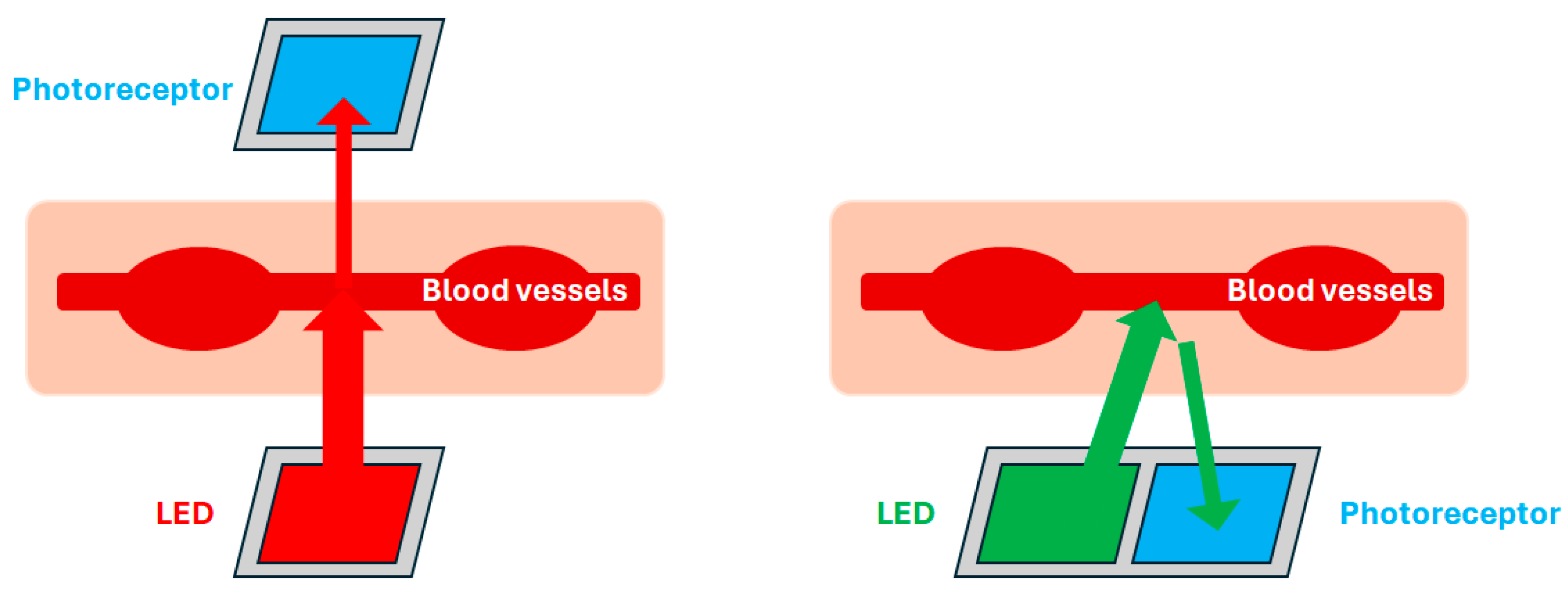
Figure 2.
Experimental setup during data recording.
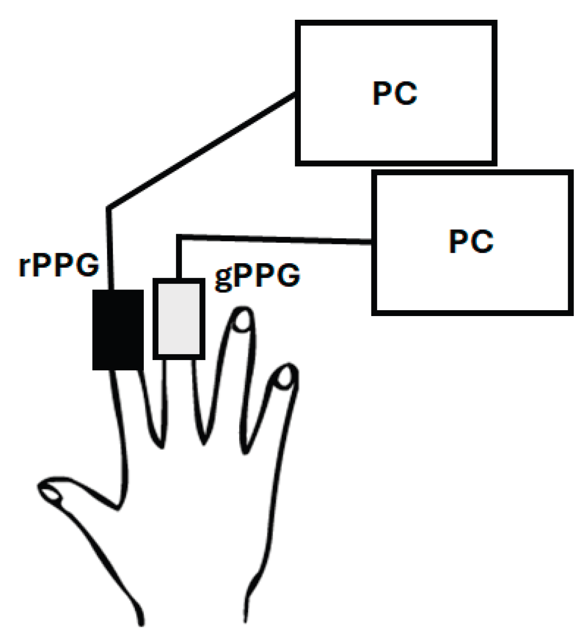
Figure 3.
An example of the amplitude spectrum (gPPG).
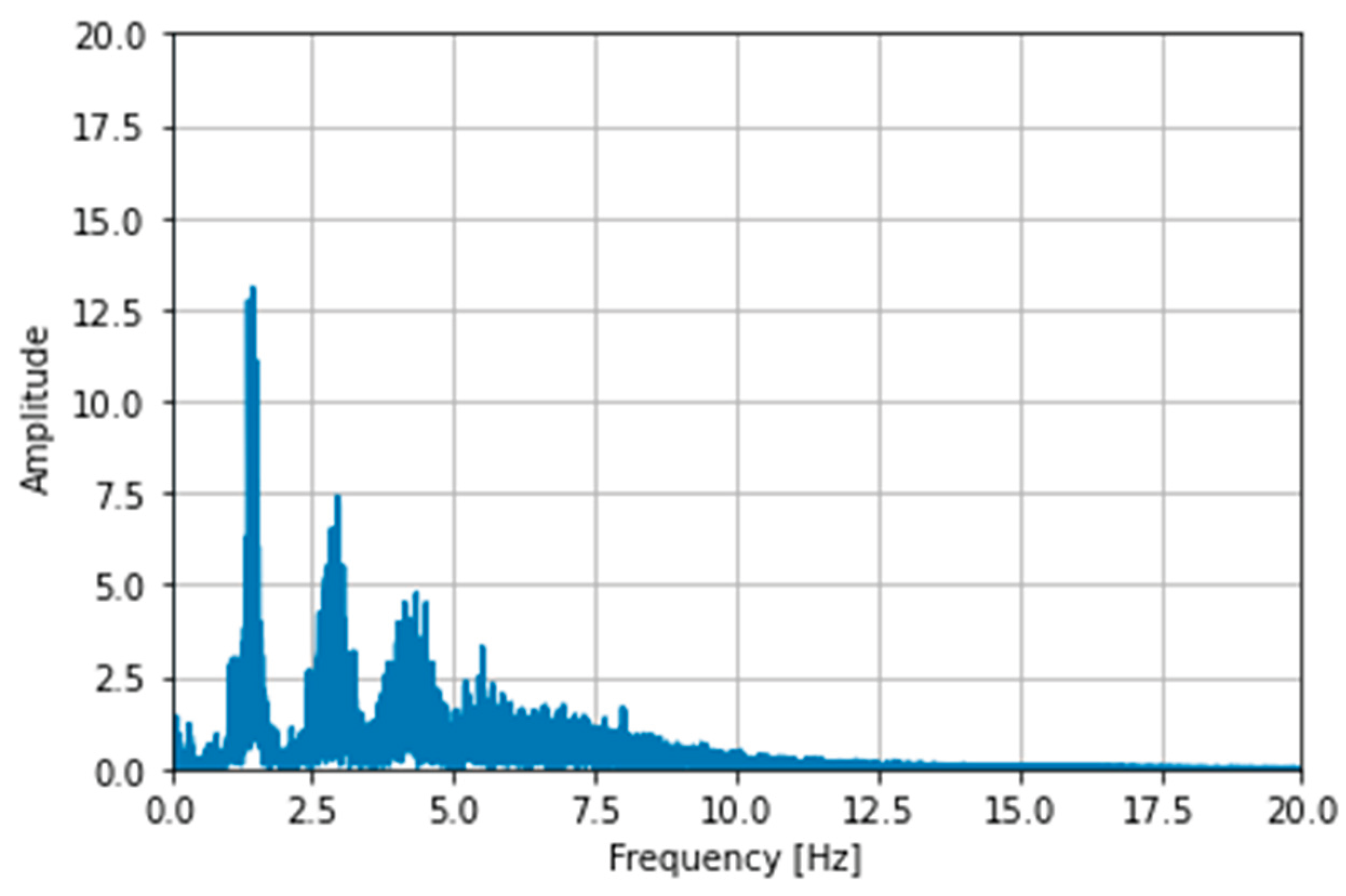
Figure 4.
Frequency response of the Butterworth filter (highcut = 0.04Hz, lowcut = 6Hz).
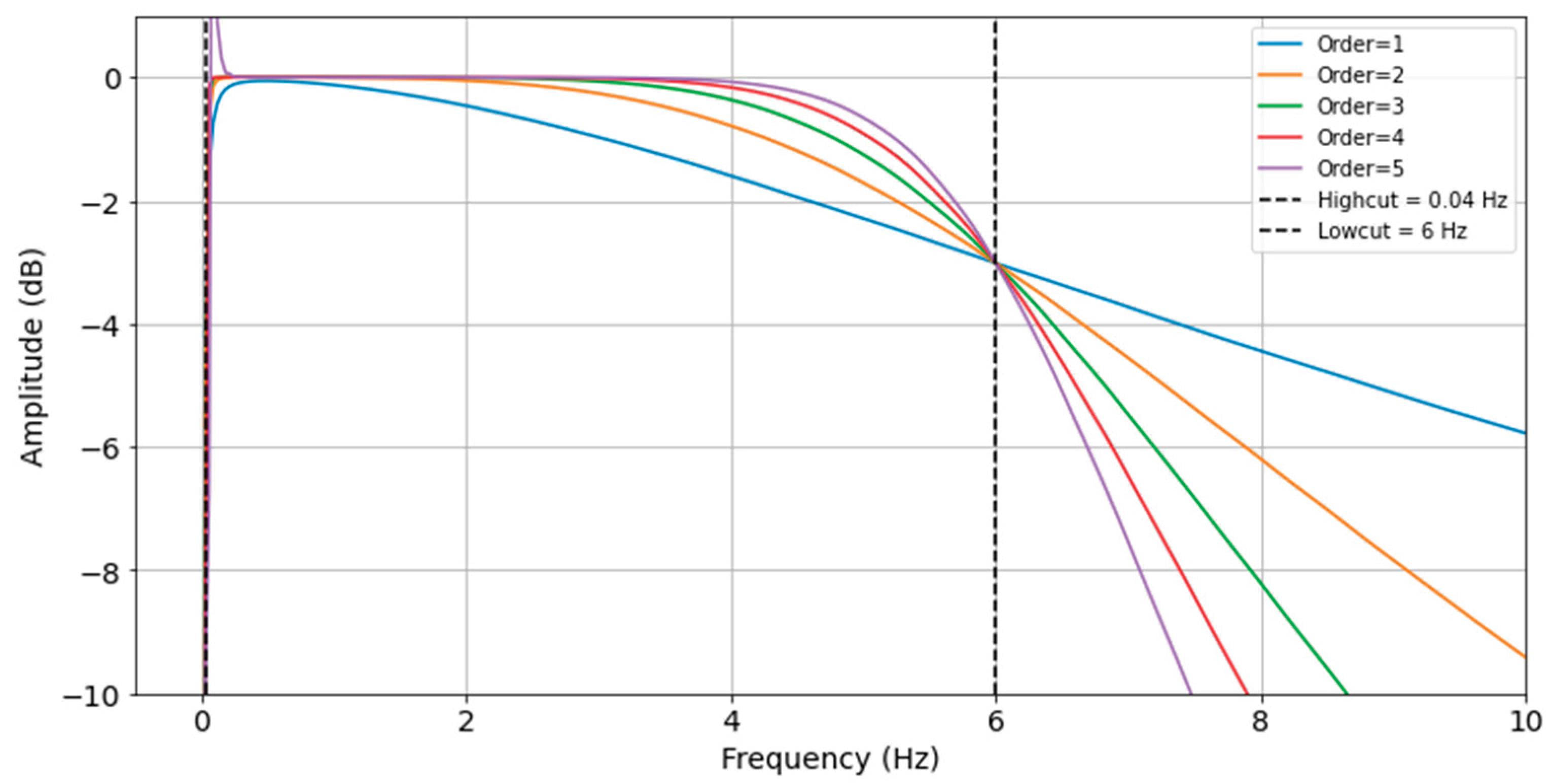
Figure 5.
Example of noise processing for the gPPG signal: (top) before processing; (bottom) after filter processing.
Figure 5.
Example of noise processing for the gPPG signal: (top) before processing; (bottom) after filter processing.
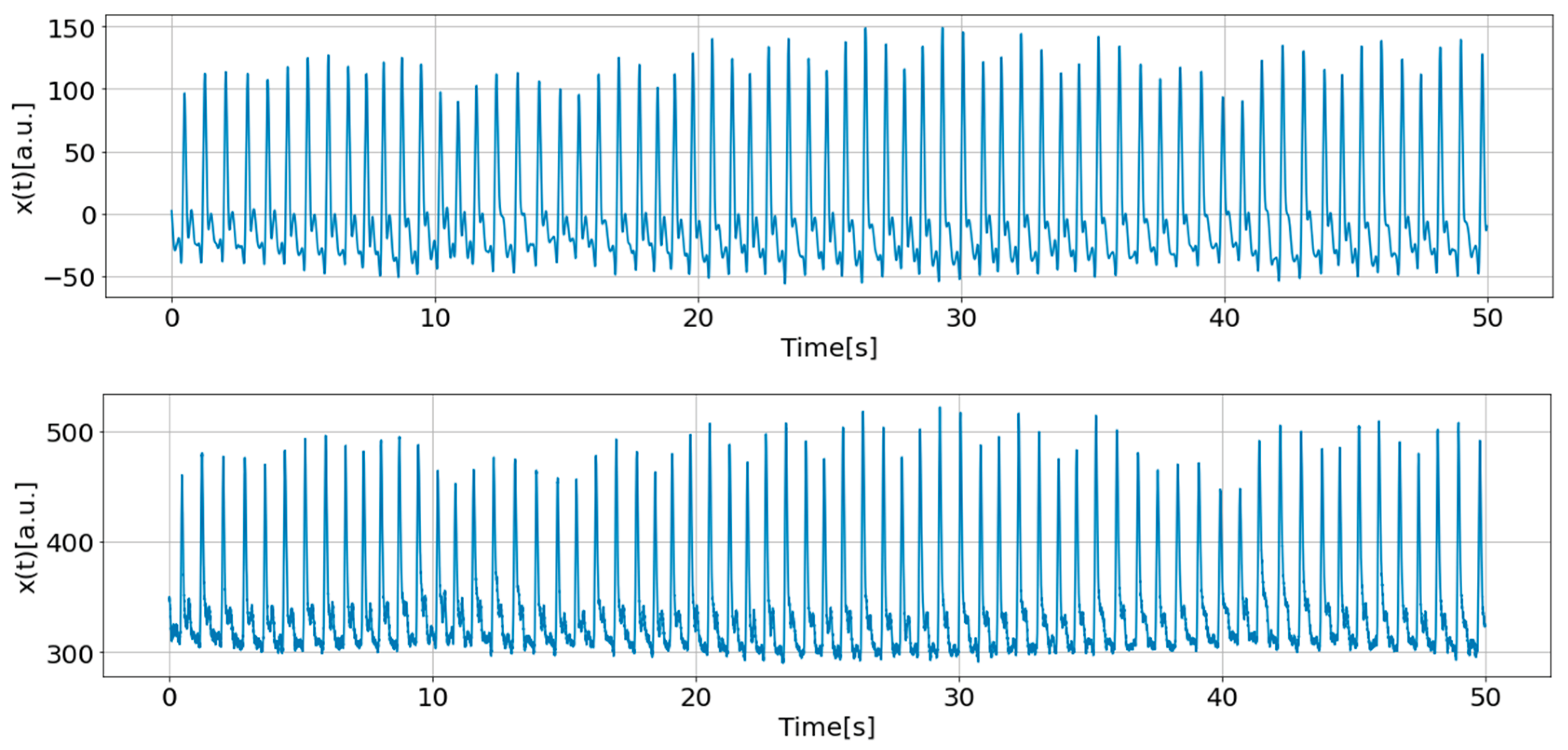
Figure 6.
Example of noise processing for the rPPG signal: (top) unprocessed; (bottom) filtered.
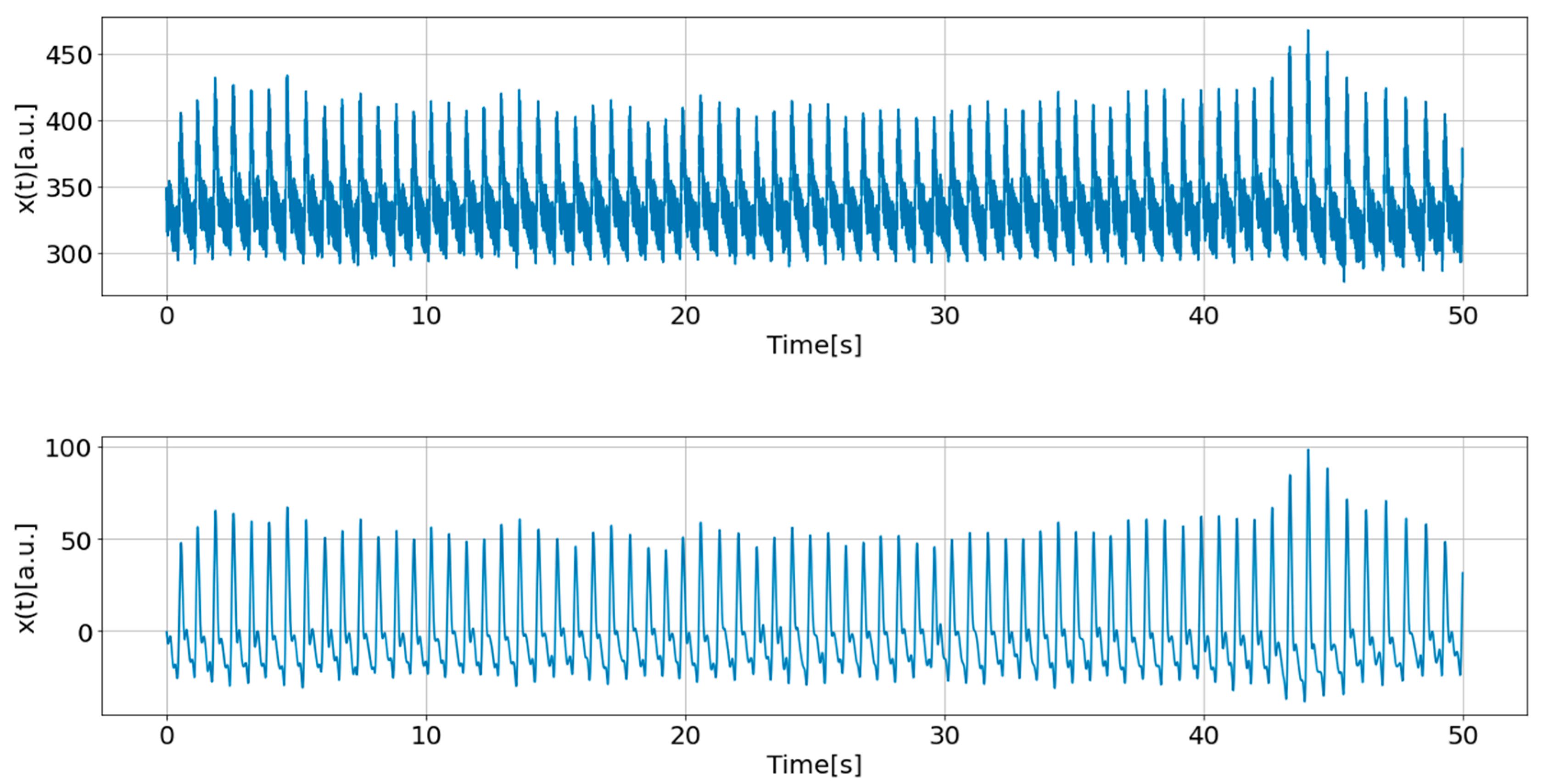
Figure 7.
An example of a normally measured PPG time: (top) Skewness; (bottom) part of PPG data.
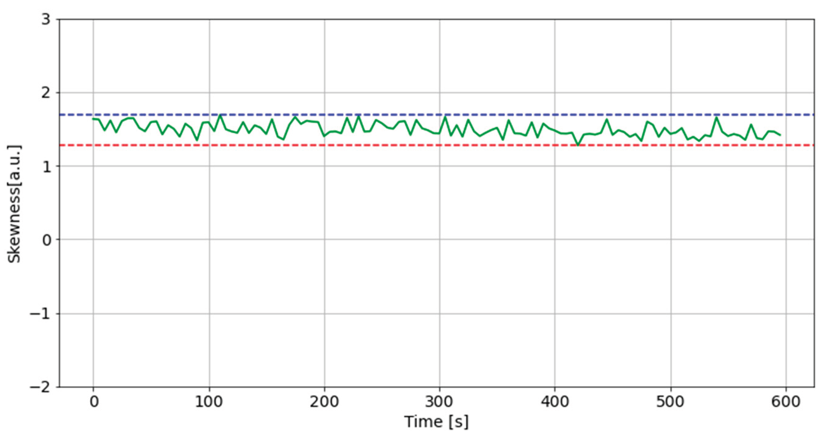
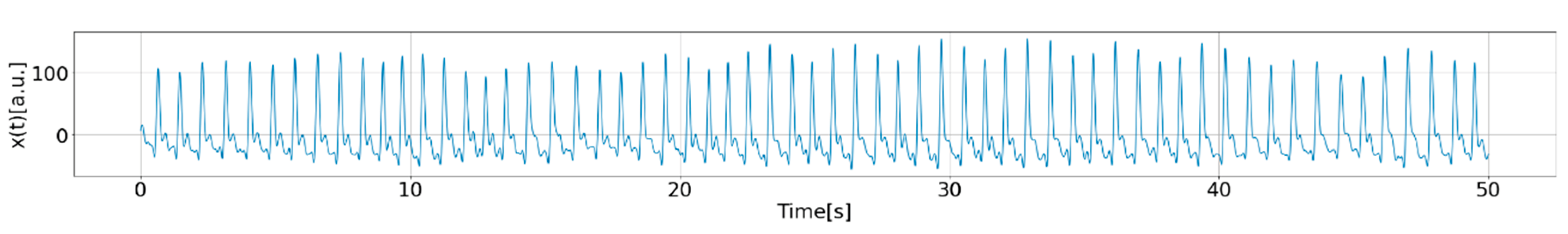
Figure 8.
An example of PPG time series measurement failure: (top) Skewness; (bottom) part of PPG data.
Figure 8.
An example of PPG time series measurement failure: (top) Skewness; (bottom) part of PPG data.
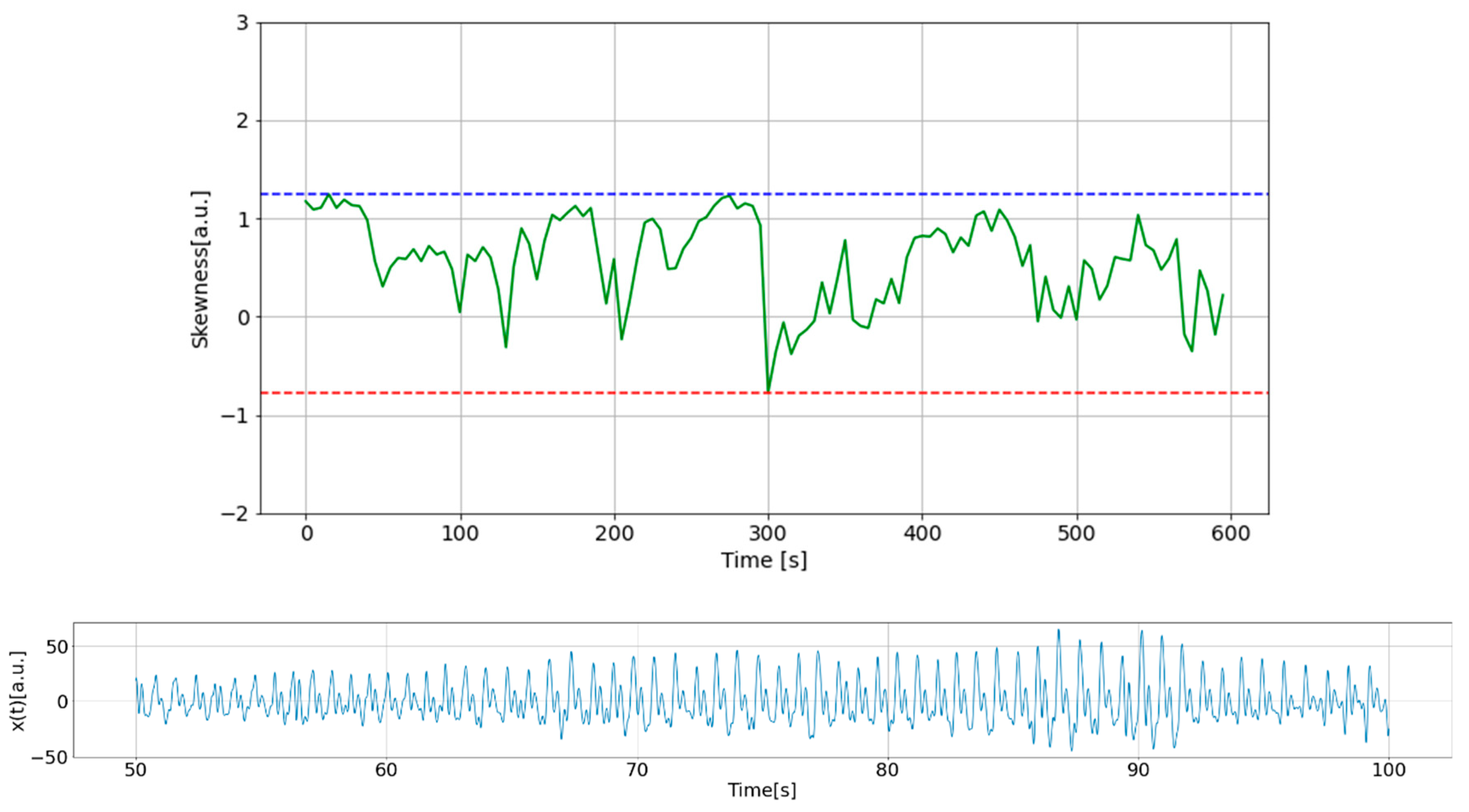
Figure 9.
Typical PPG waveform.
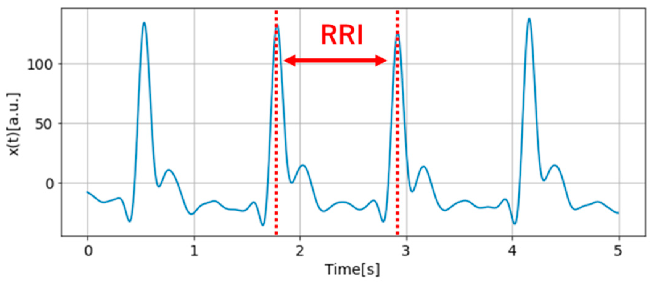
Figure 10.
Example of detecting the maximum peaks.
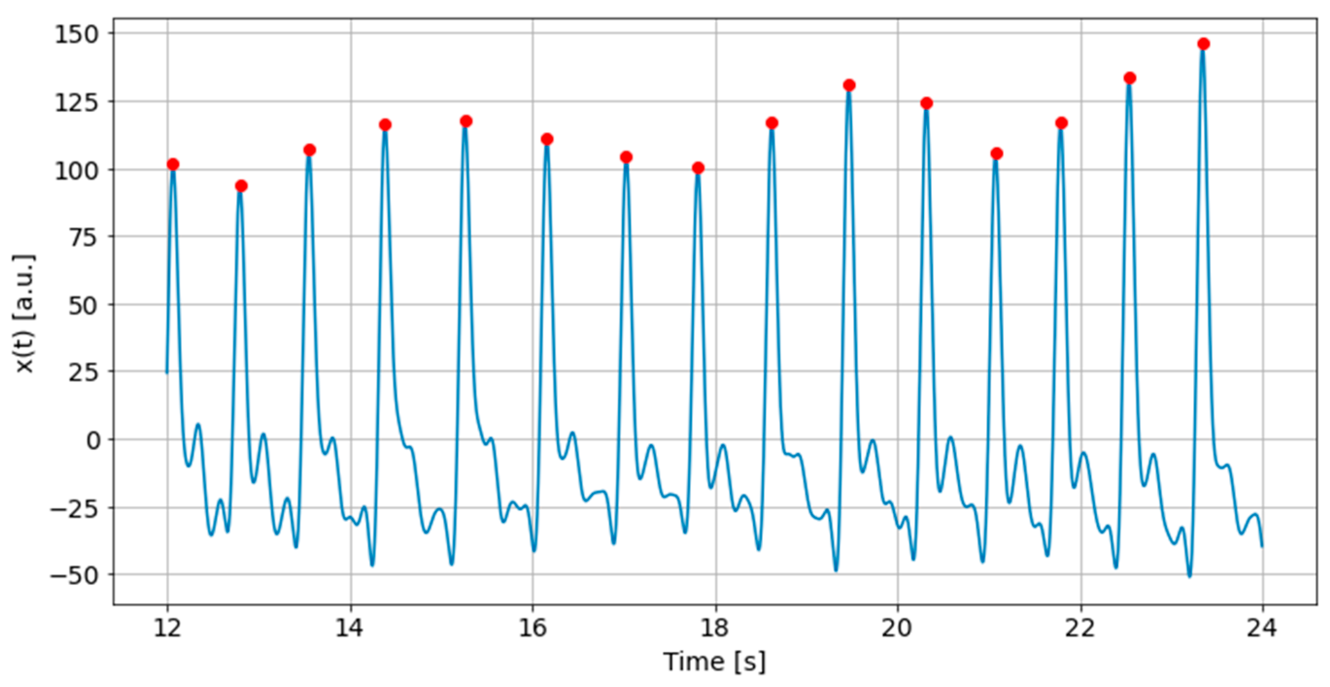
Figure 11.
An example of heart rate variability estimation: (a) RRI; (b) heart rate.
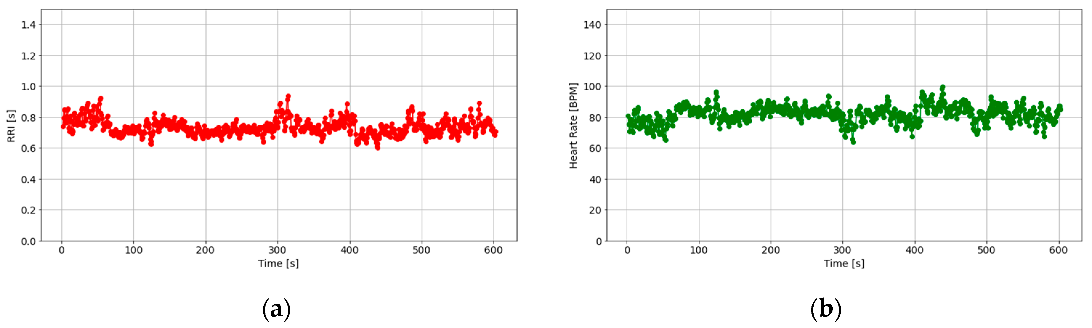
Figure 12.
An example of LF/HF of a stable measurement.
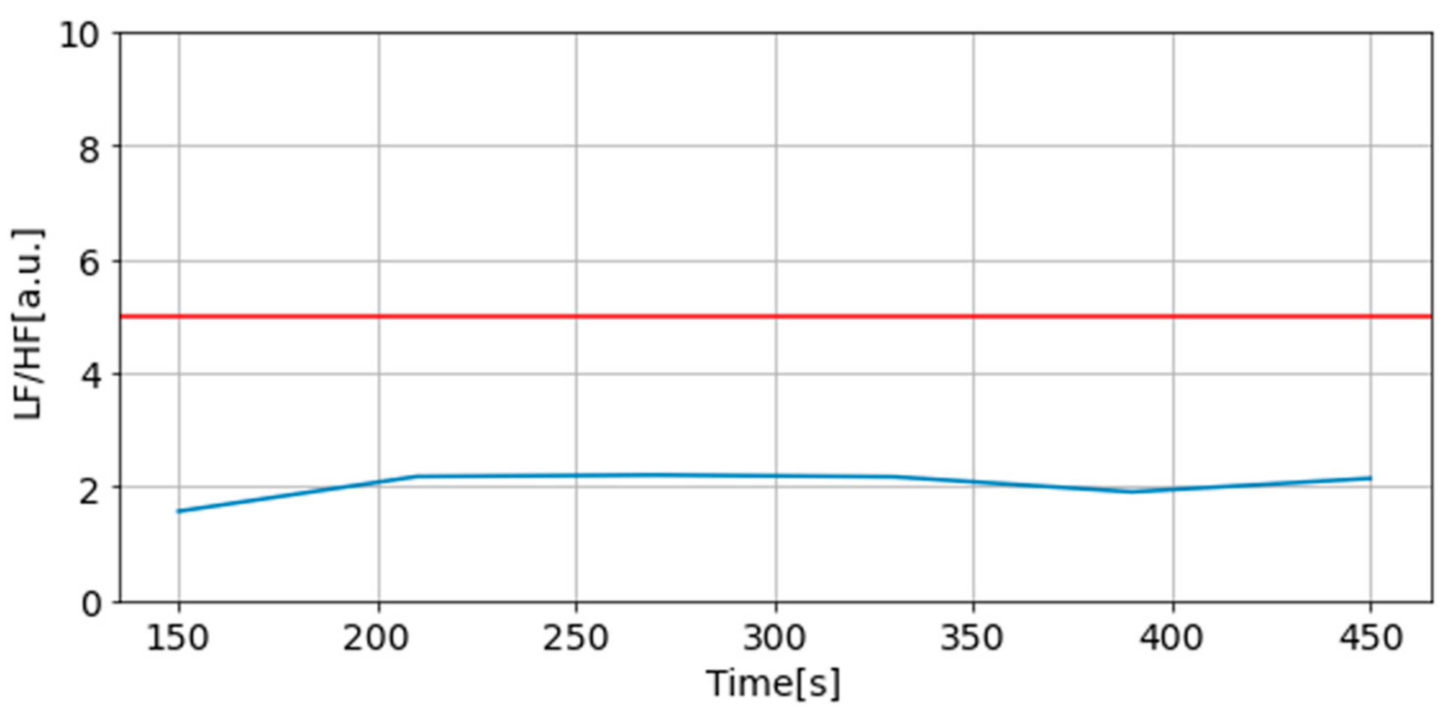
Figure 13.
An example of LF/HF of an unstable measurement.
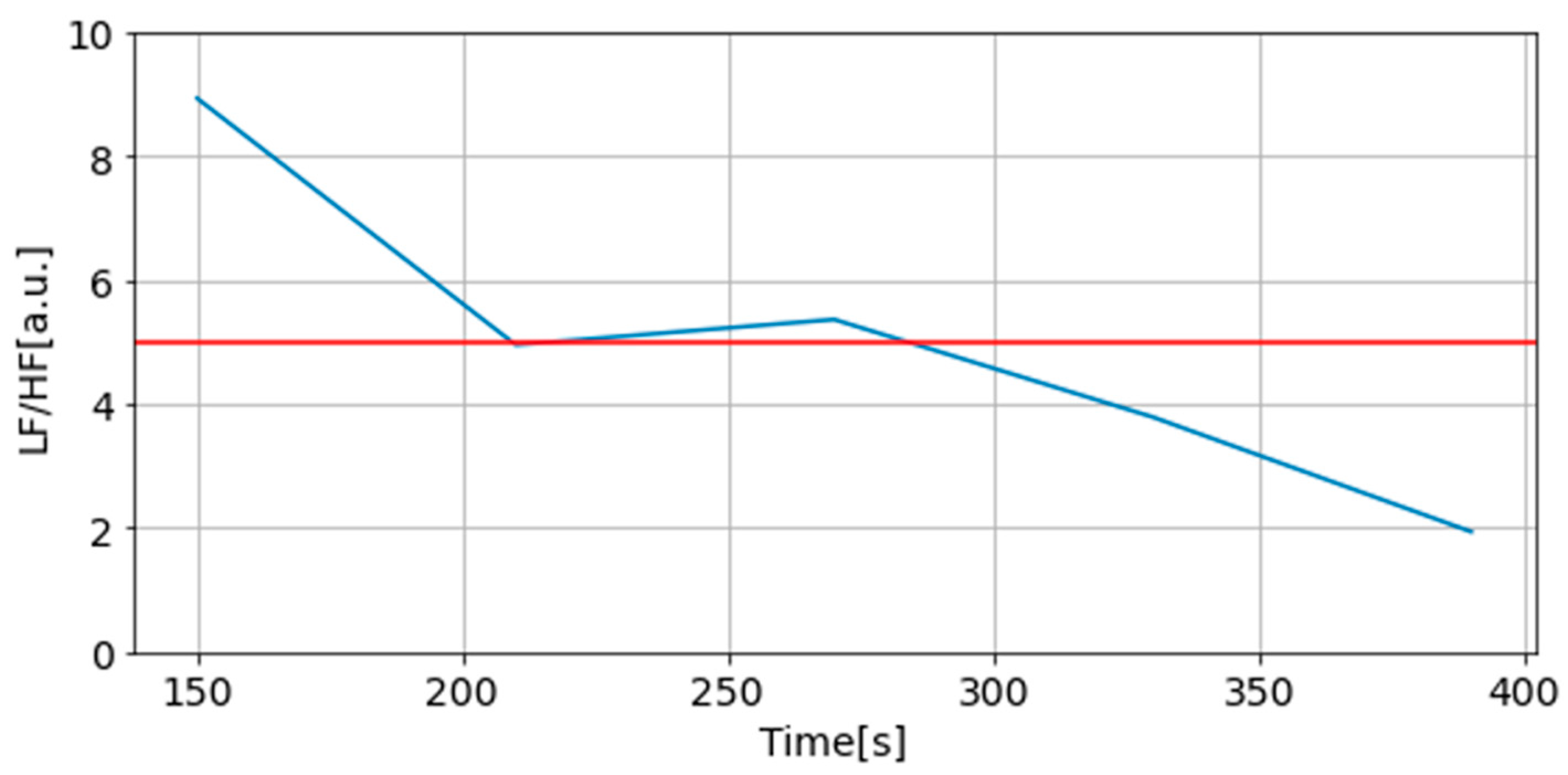
Figure 14.
An example of Poincaré: (a) 60~180 points; (b) 180~300 points; (c) 300~420 points; (d) 420~540 points.
Figure 14.
An example of Poincaré: (a) 60~180 points; (b) 180~300 points; (c) 300~420 points; (d) 420~540 points.
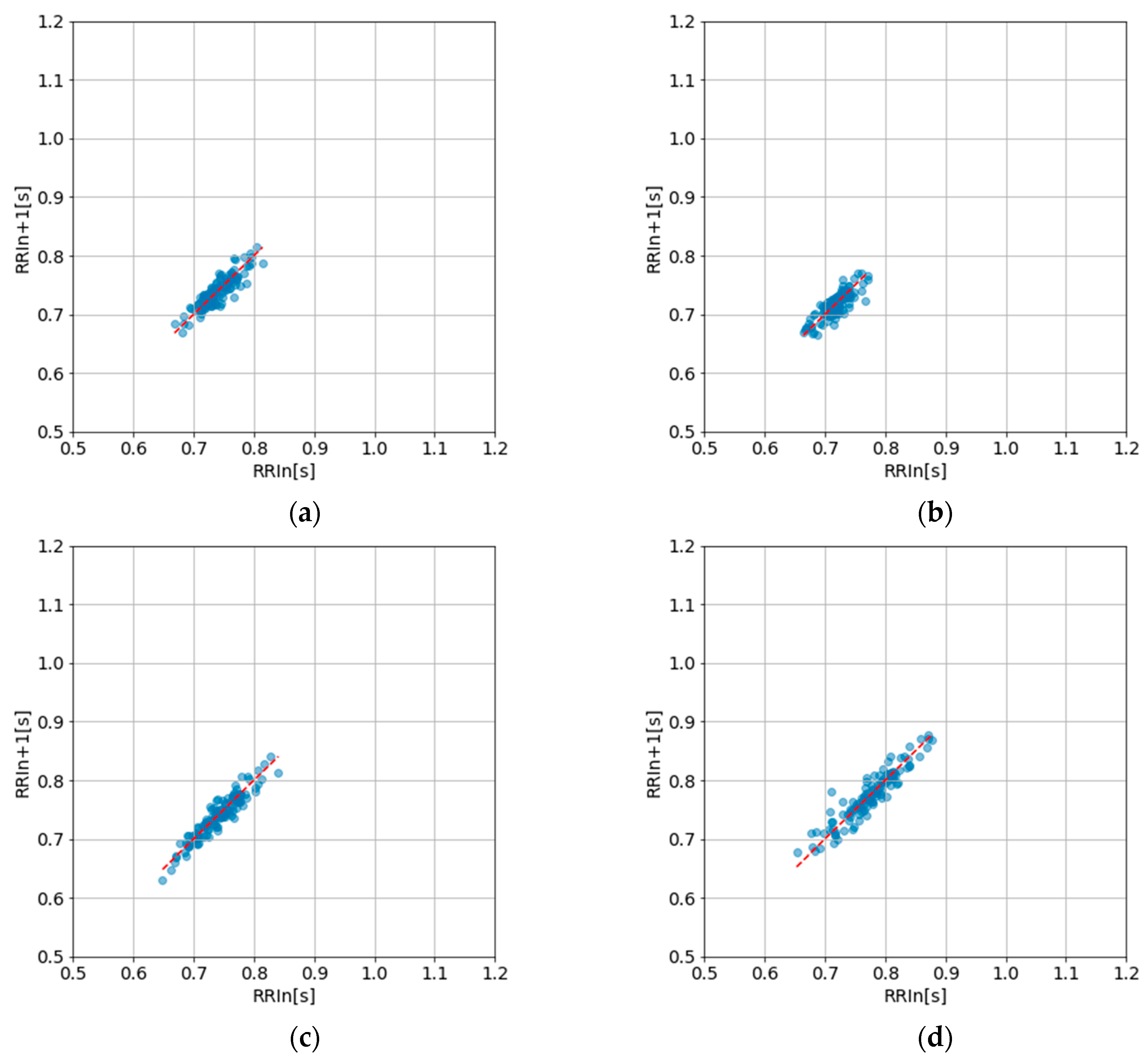
Figure 15.
An example of sd2/sd1 obtained from a stable measurement.
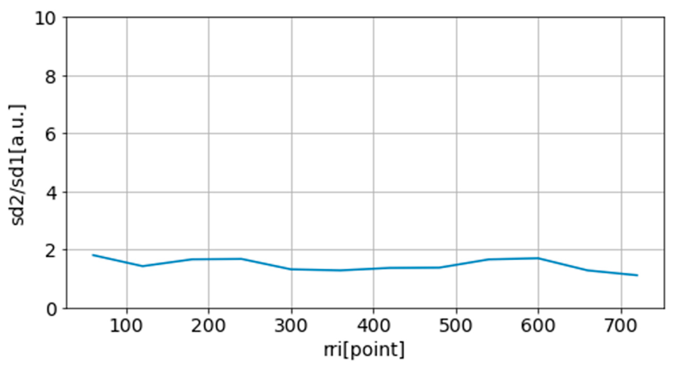
Figure 16.
An example of sd2/sd1 obtained from an unstable measurement.
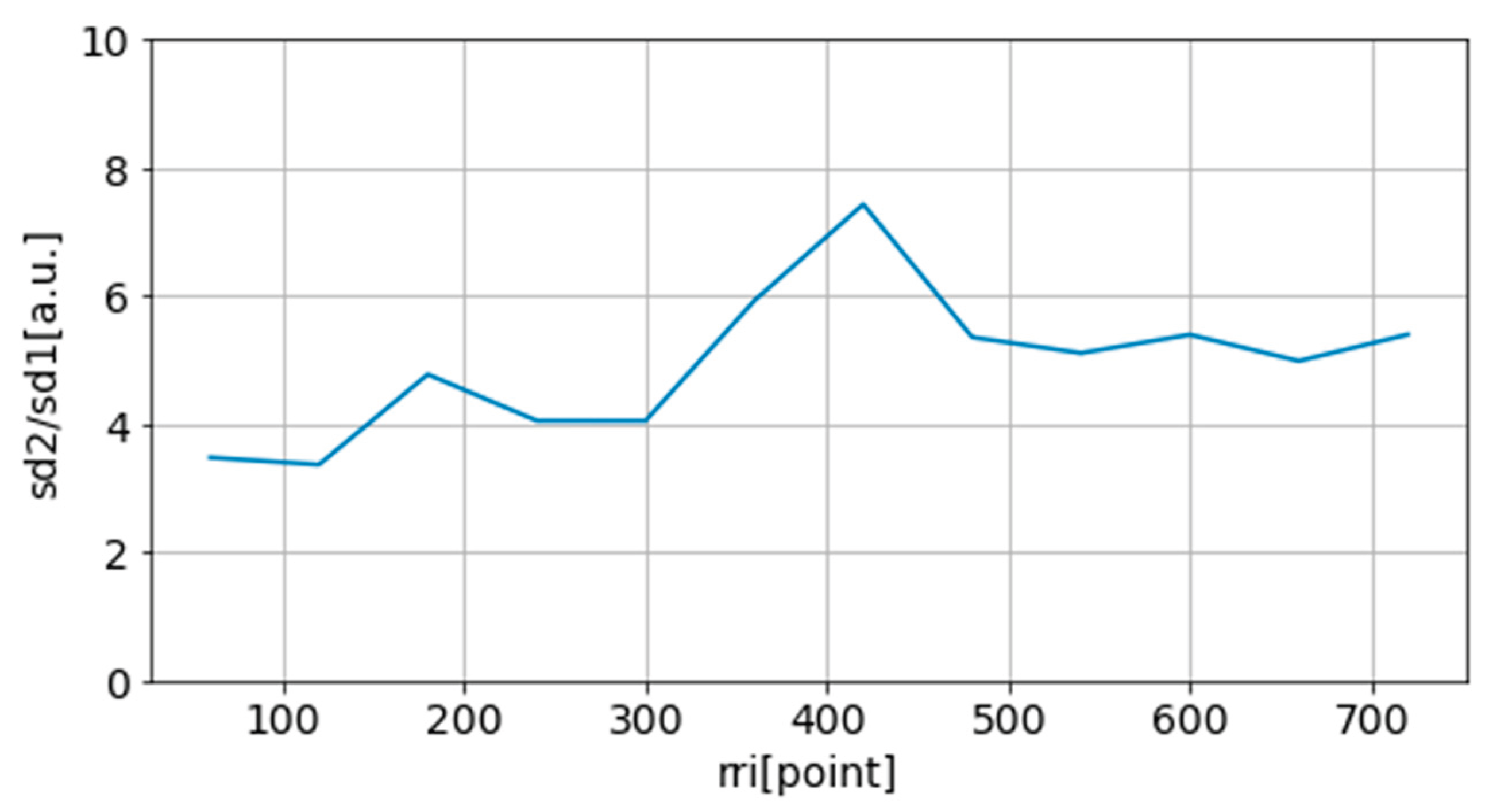
Figure 17.
An example of the PPG waveform of the PPG data (10 sec) at 400 Hz. 200 Hz, and 100 Hz sampling frequency.
Figure 17.
An example of the PPG waveform of the PPG data (10 sec) at 400 Hz. 200 Hz, and 100 Hz sampling frequency.
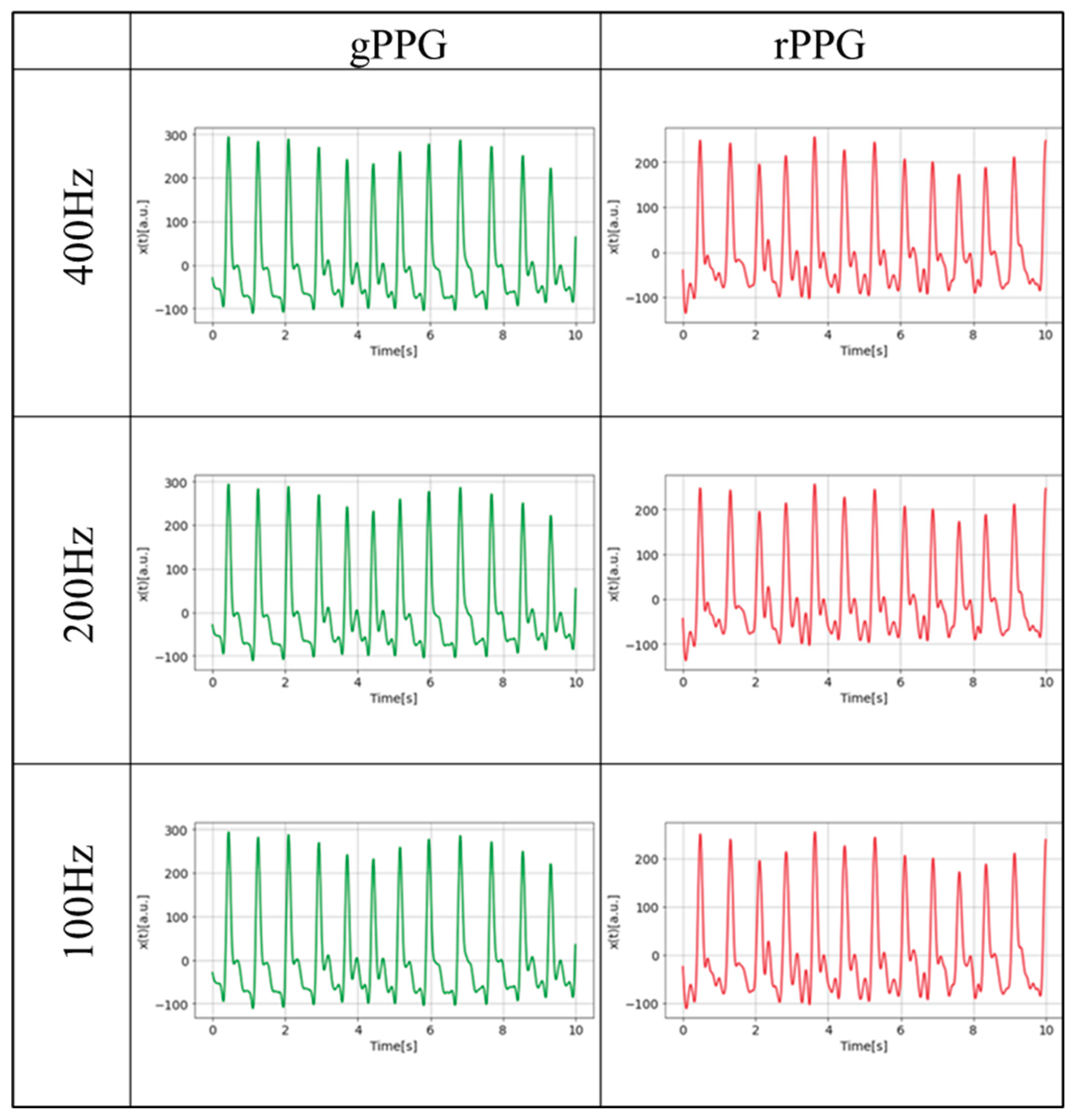
Figure 18.
An example of the autocorrelation graph of the gPPG.
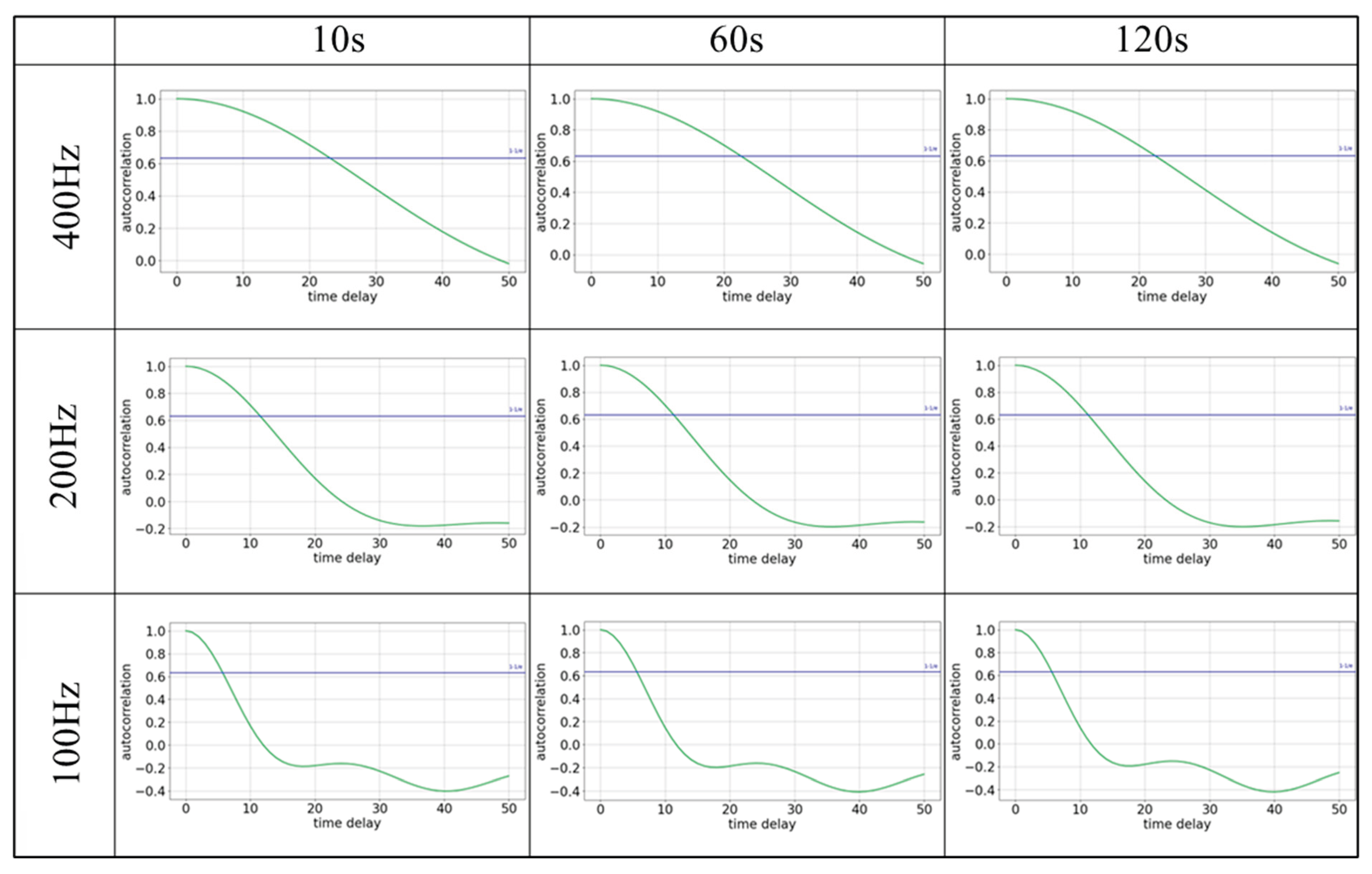
Figure 19.
An example of the autocorrelation graph of the rPPG.
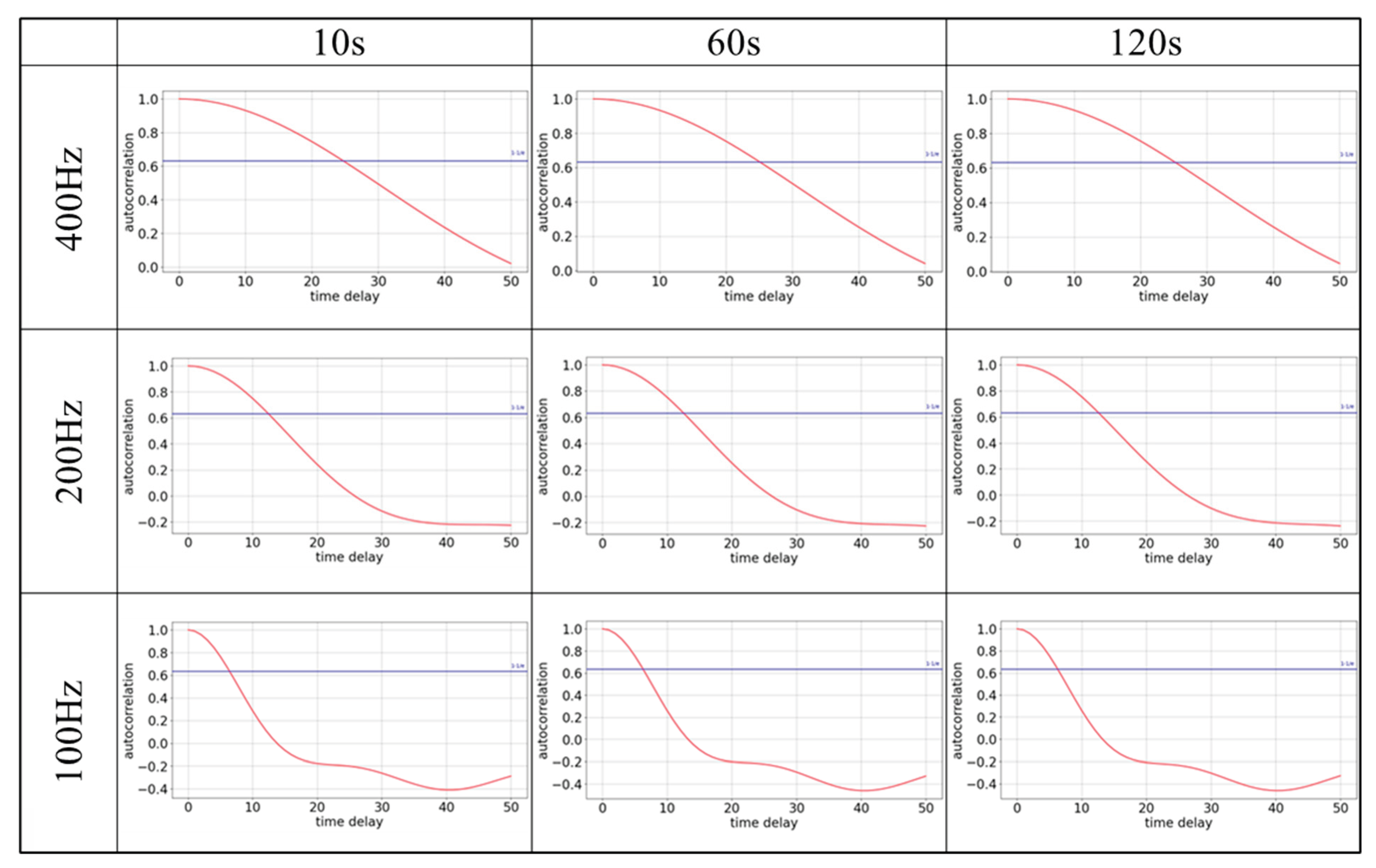
Figure 20.
An example of dimension estimation by the false neighborhood method for gPPG.
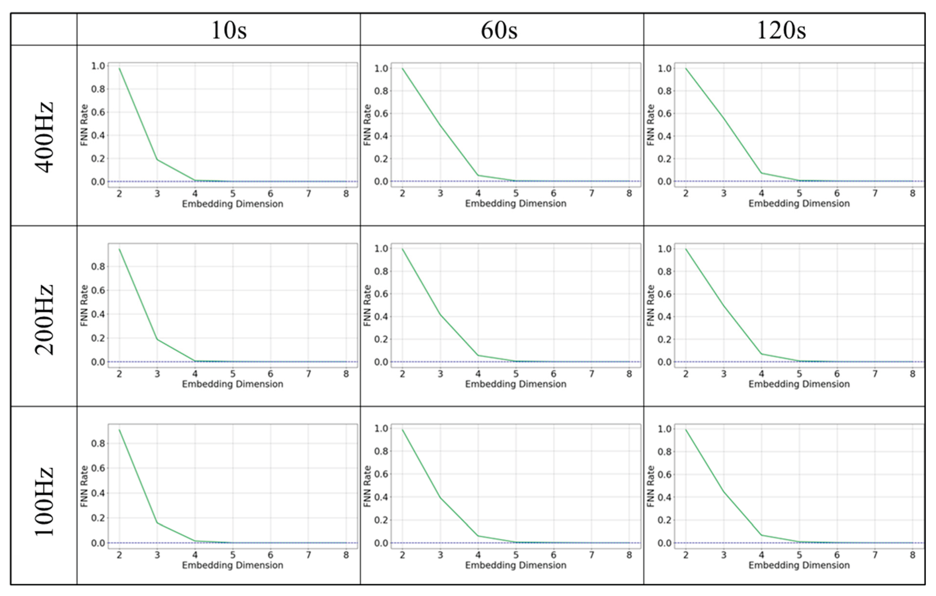
Figure 21.
An example of dimension estimation by the false neighborhood method for rPPG.
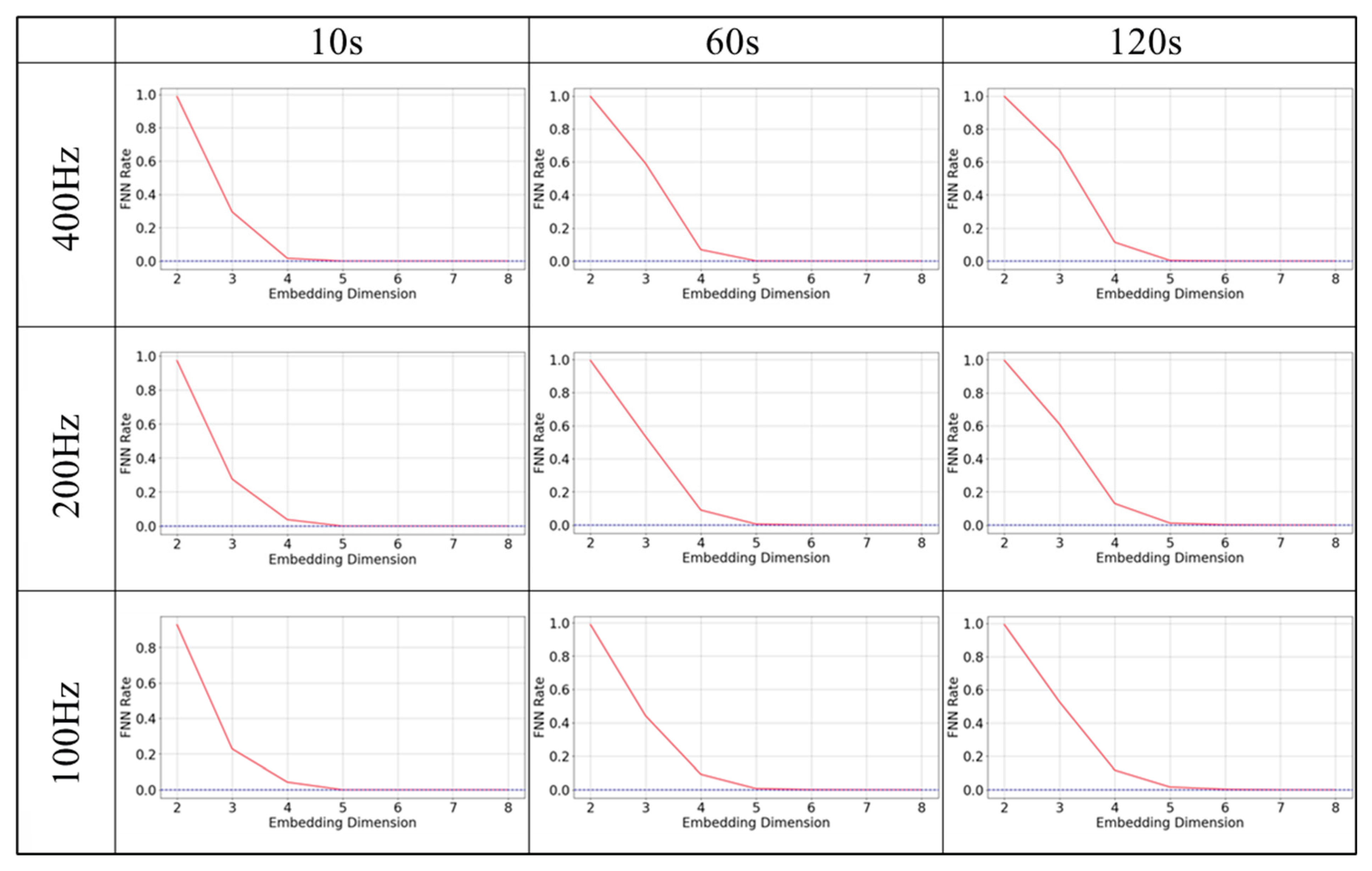
Figure 22.
An example of the reconstructed attractor for the gPPG data subsets.
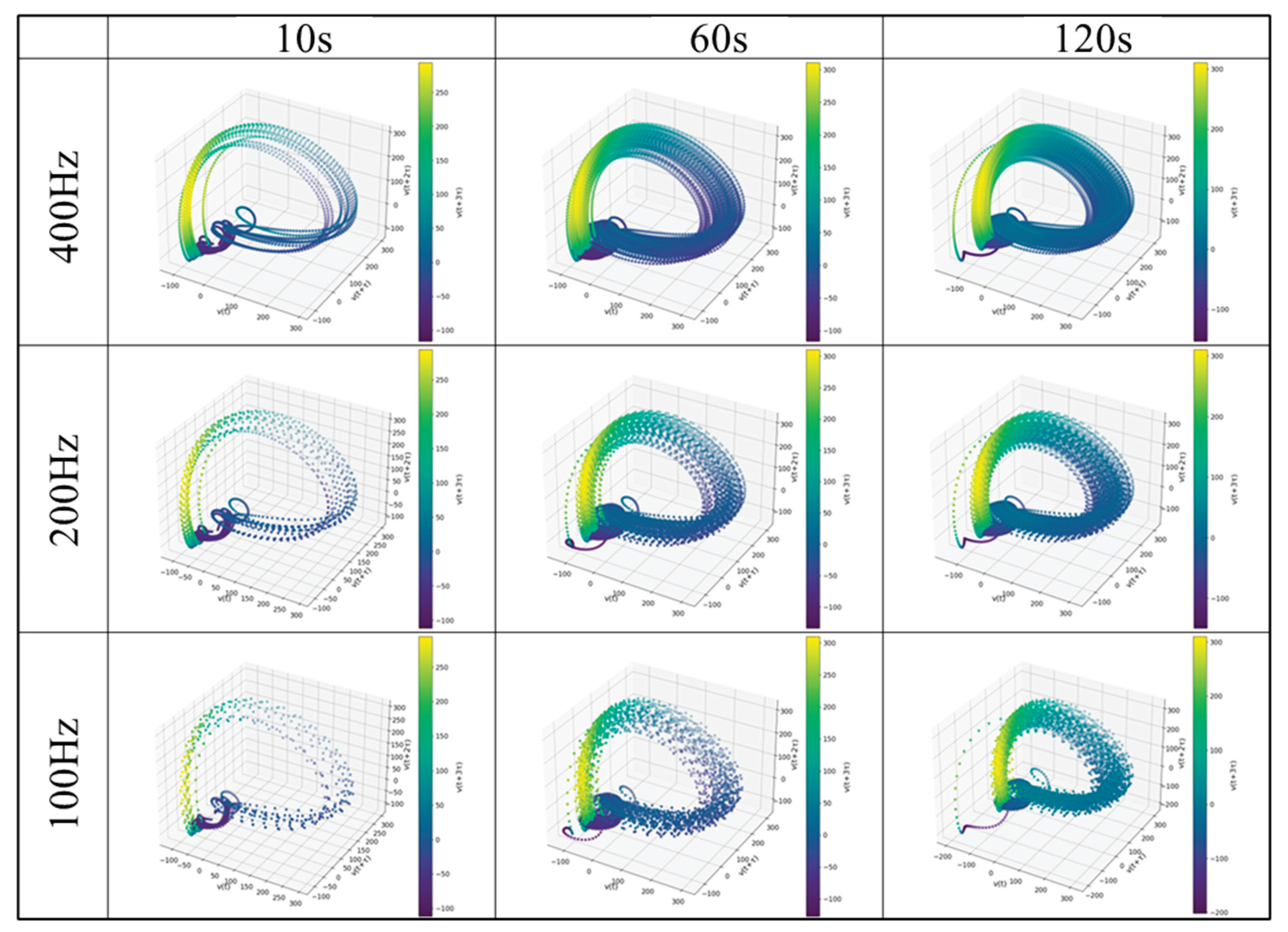
Figure 23.
An example of the reconstructed attractor for the rPPG data subsets.
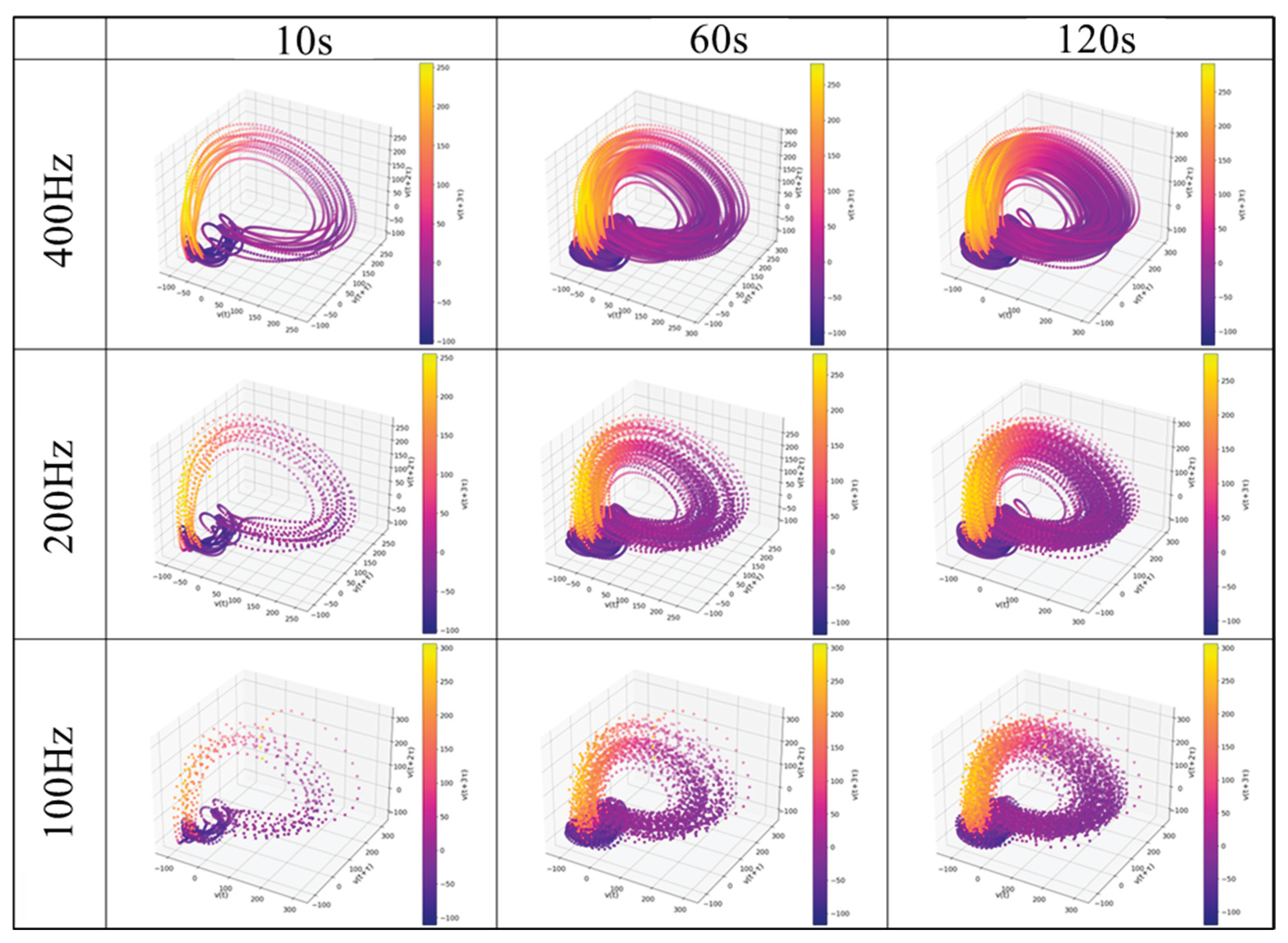
Figure 24.
An example of the RP for the gPPG data subsets.
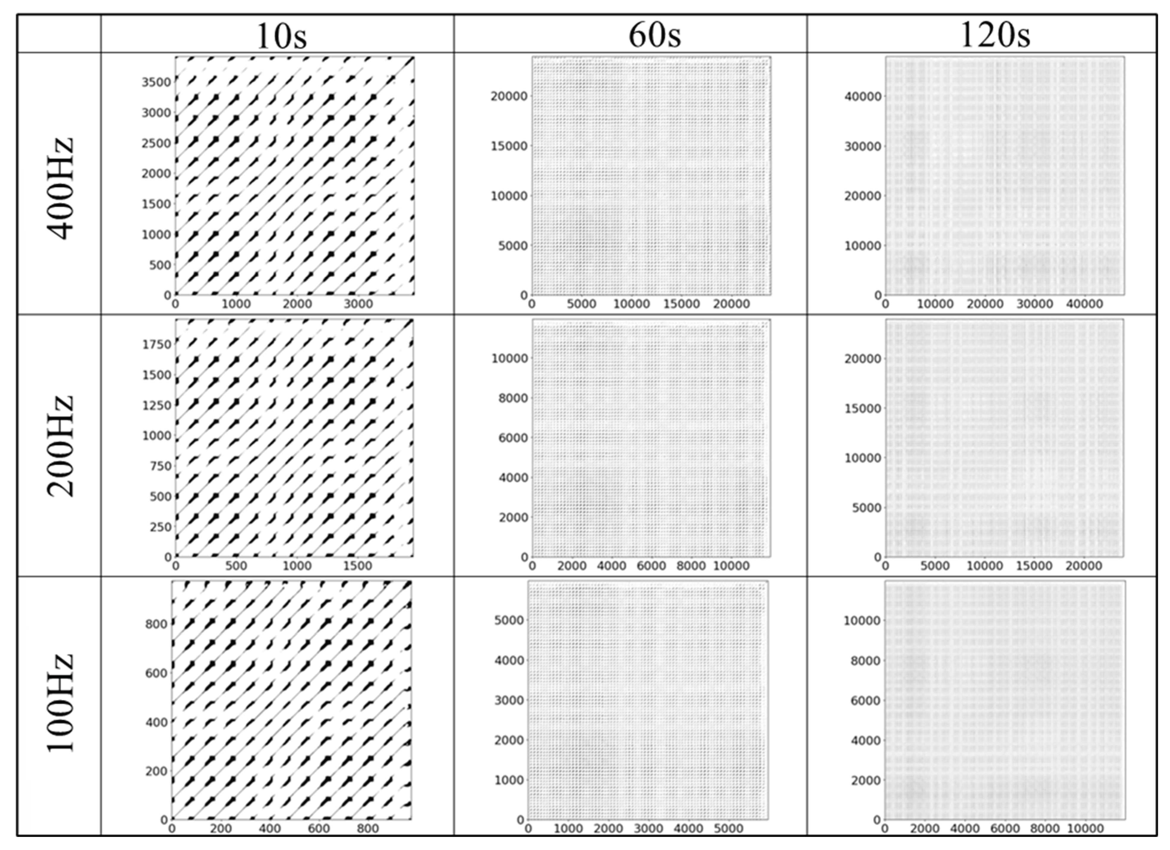
Figure 25.
An example of the RP for the rPPG data subsets.
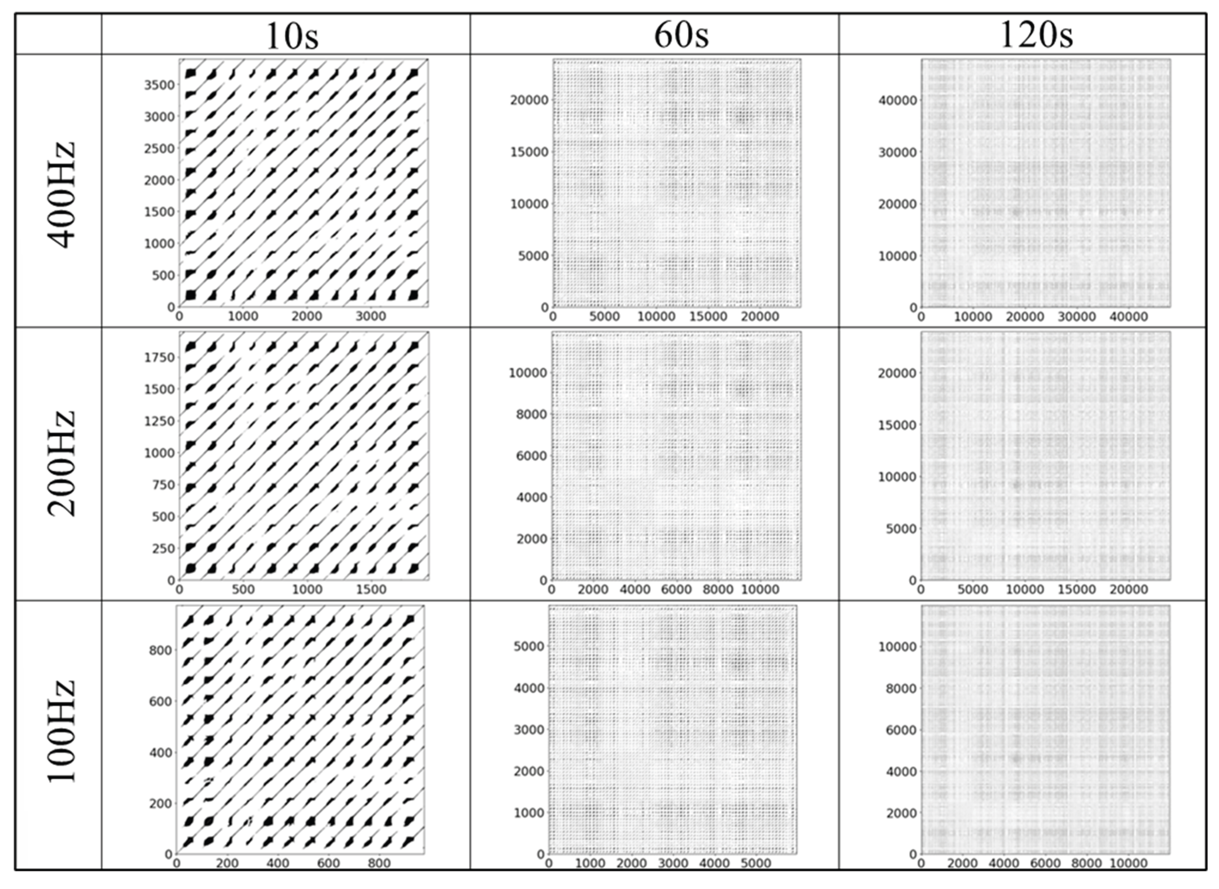
Figure 26.
An example of the variation of the RQA indexes of the gPPG (400 Hz with 200 seconds time series length).
Figure 26.
An example of the variation of the RQA indexes of the gPPG (400 Hz with 200 seconds time series length).
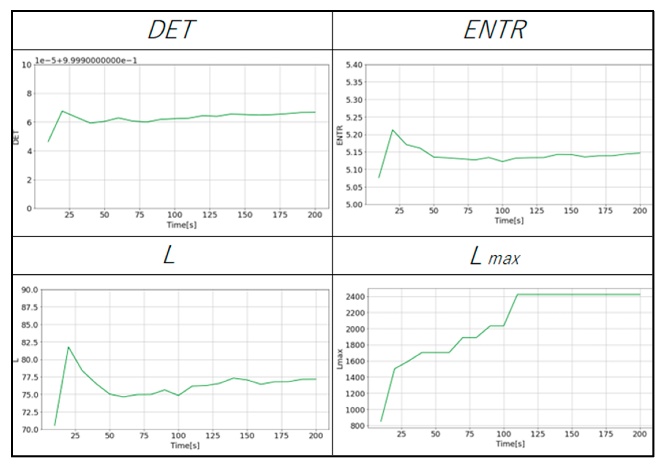
Figure 27.
An example of the variation of the RQA indexes of the rPPG (400 Hz with 200 seconds time series length).
Figure 27.
An example of the variation of the RQA indexes of the rPPG (400 Hz with 200 seconds time series length).
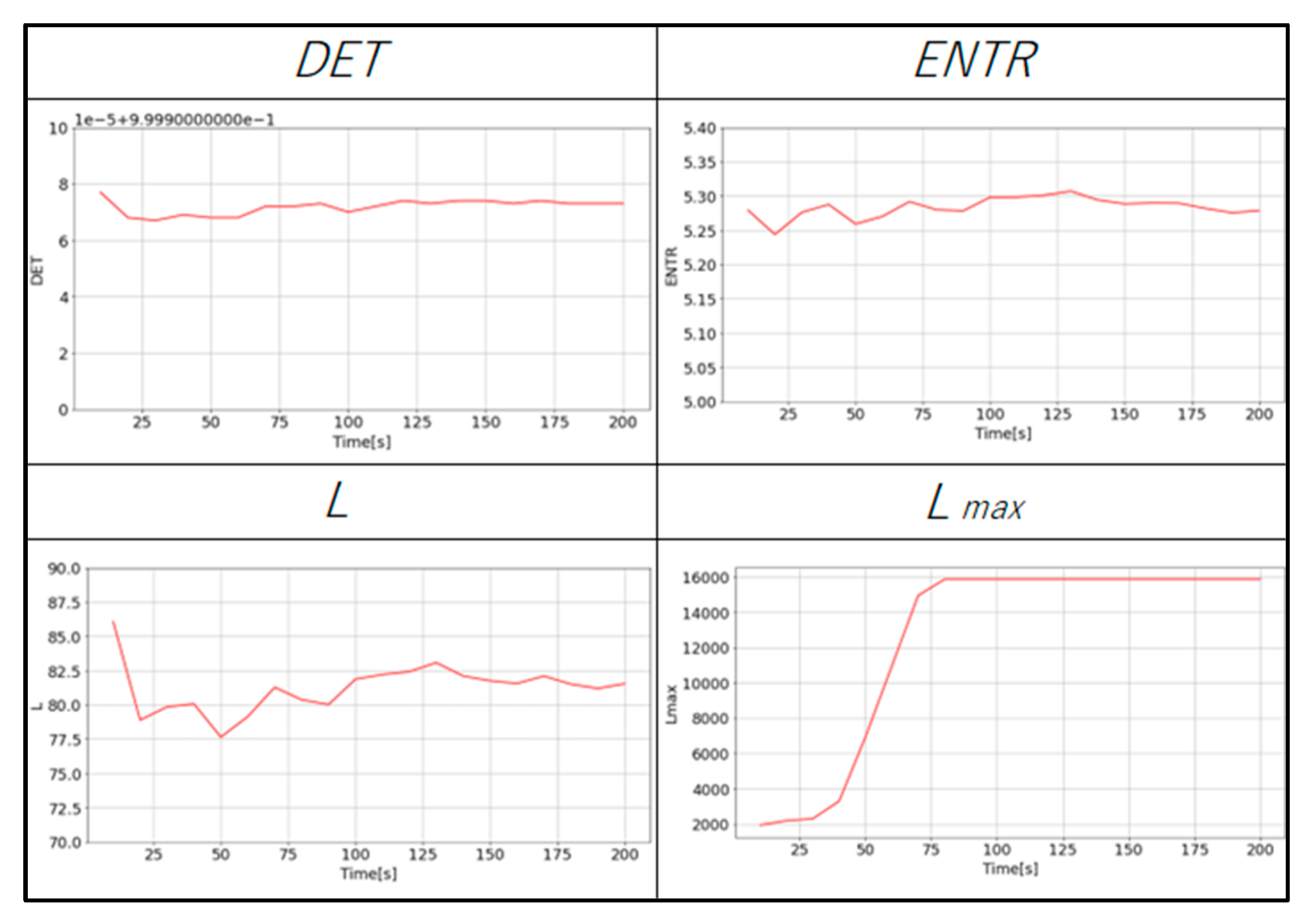
Figure 28.
Distribution of RQA indices at each frequency for gPPG.

Figure 29.
Distribution of RQA indices at each frequency for rPPG.
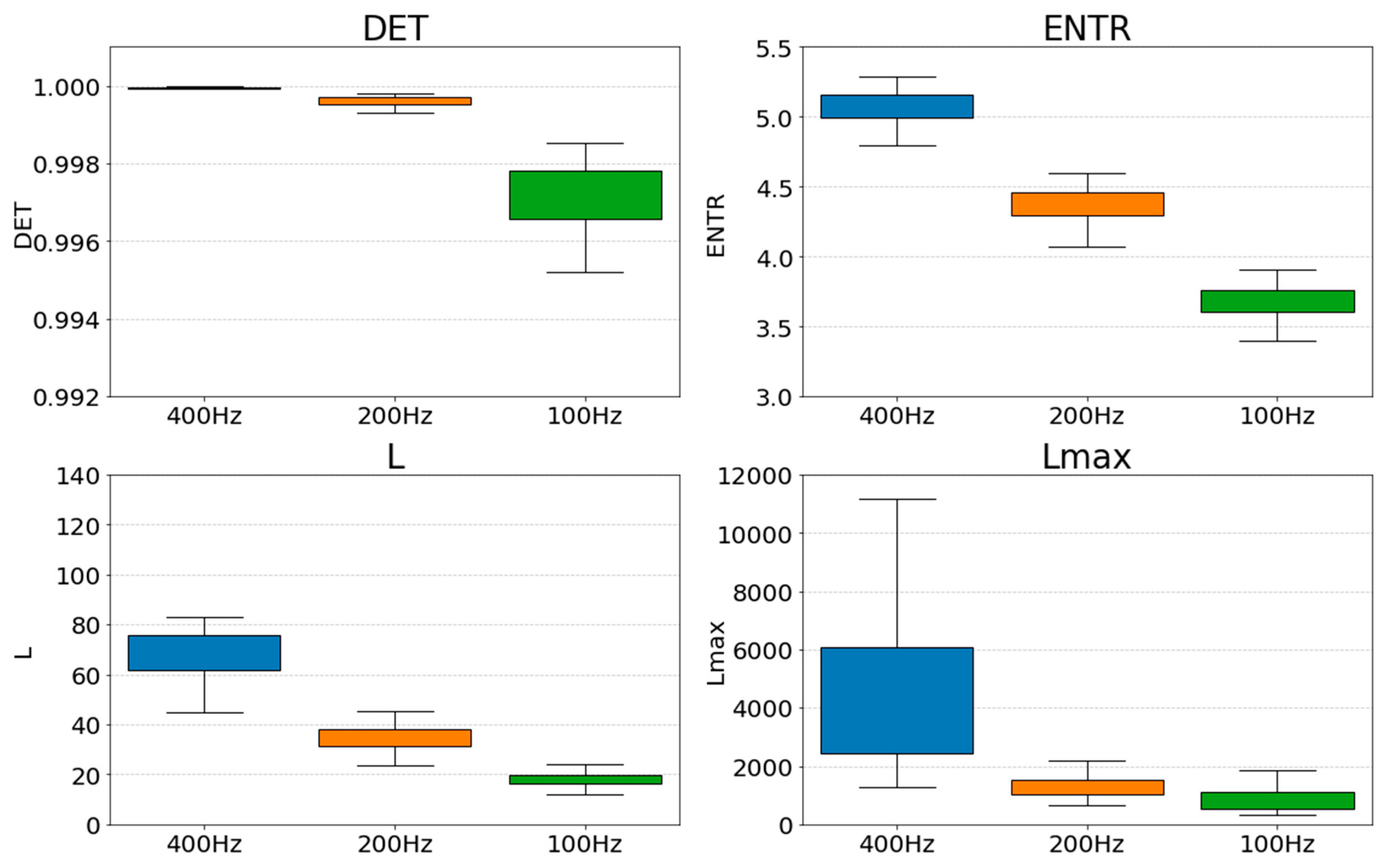
Figure 30.
Color map of the average error for variable time series length for PPG (400 Hz): (left half) gPPG; (right half) rPPG.
Figure 30.
Color map of the average error for variable time series length for PPG (400 Hz): (left half) gPPG; (right half) rPPG.
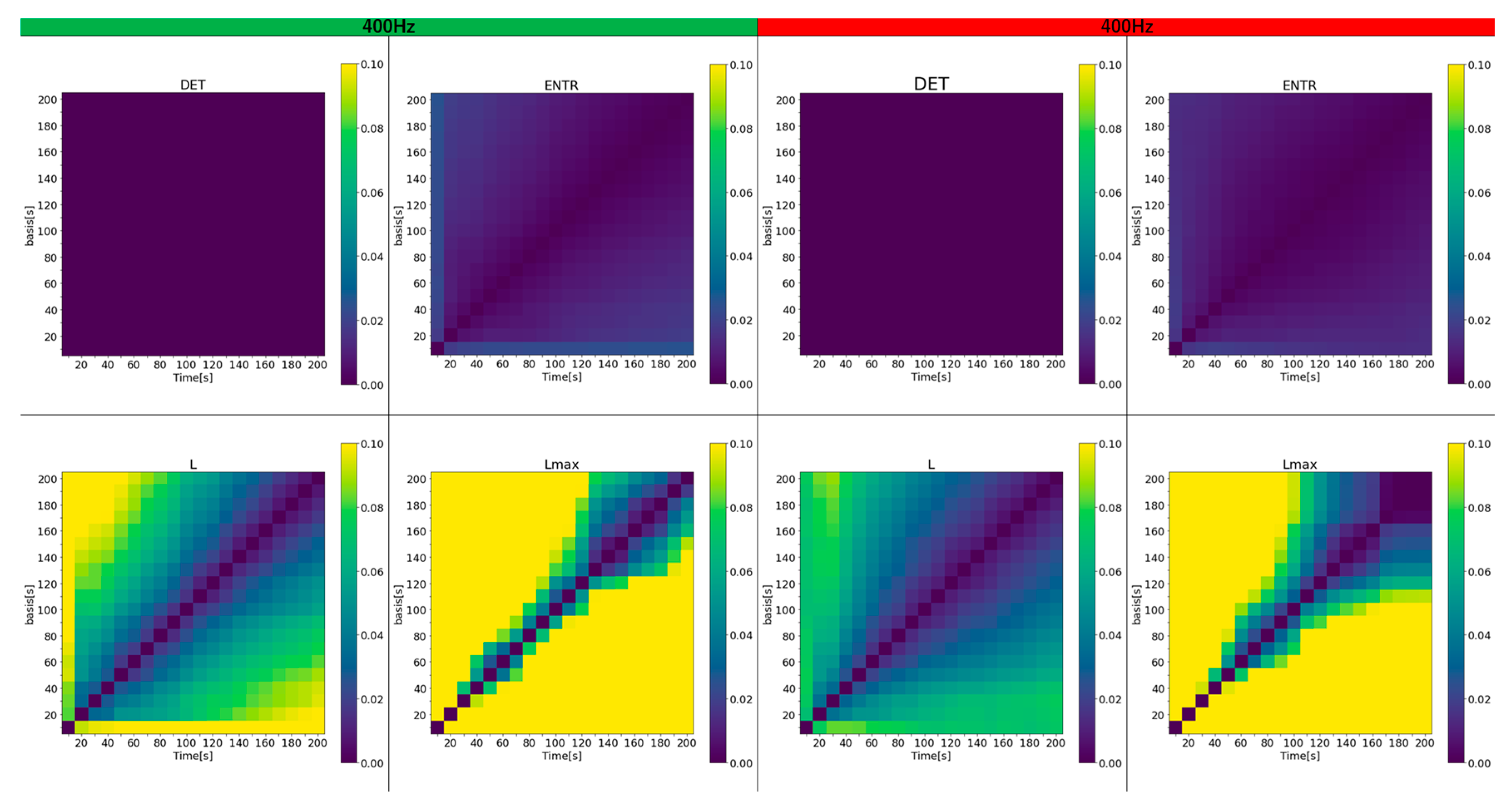
Figure 31.
Color maps of the average error for variable time series length for PPG (200Hz): (left half) gPPG; (right half) rPPG.
Figure 31.
Color maps of the average error for variable time series length for PPG (200Hz): (left half) gPPG; (right half) rPPG.
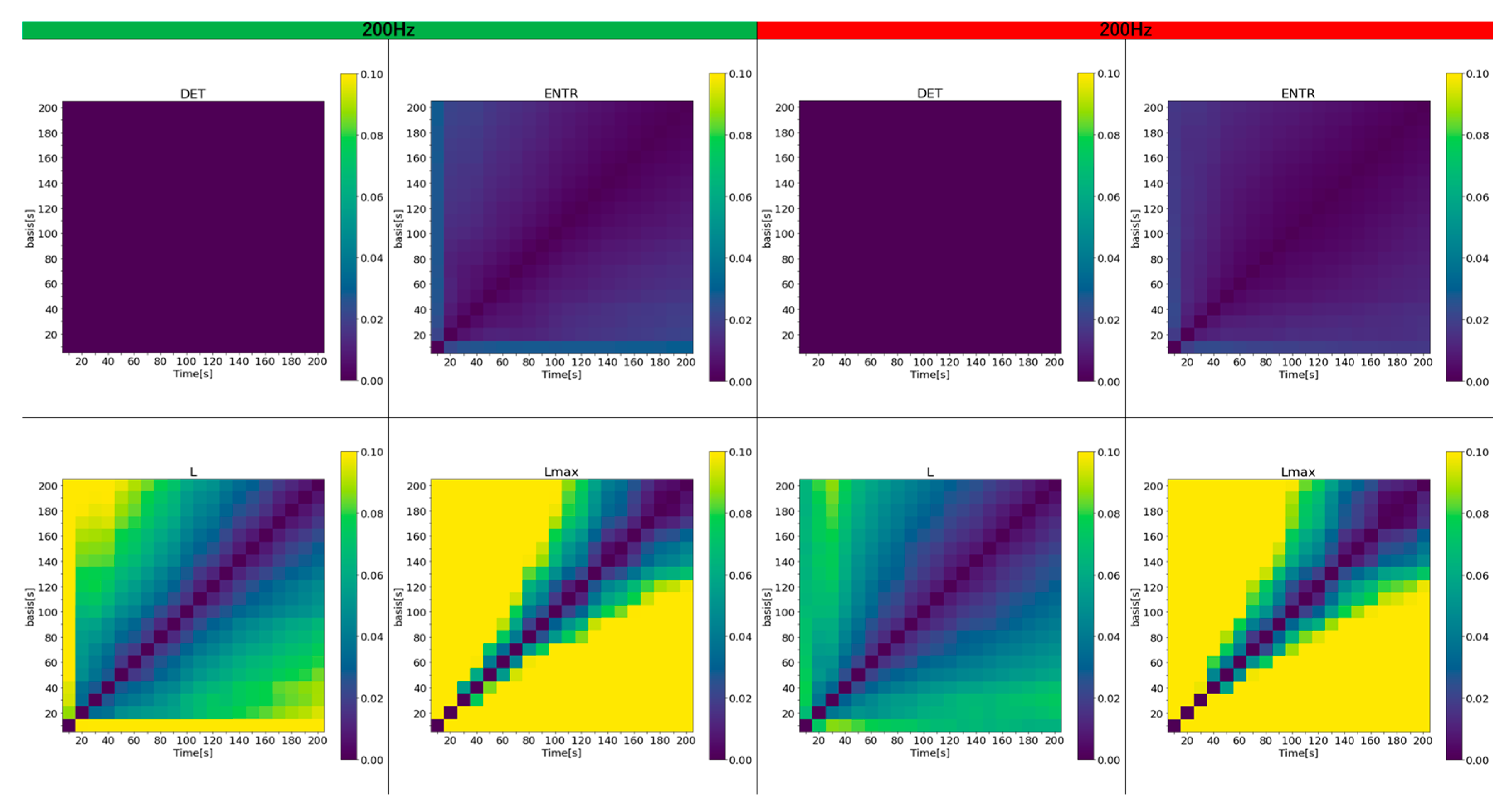
Figure 32.
Color maps of the average error for variable time series length for PPG (100Hz): (left half) gPPG; (right half) rPPG.
Figure 32.
Color maps of the average error for variable time series length for PPG (100Hz): (left half) gPPG; (right half) rPPG.
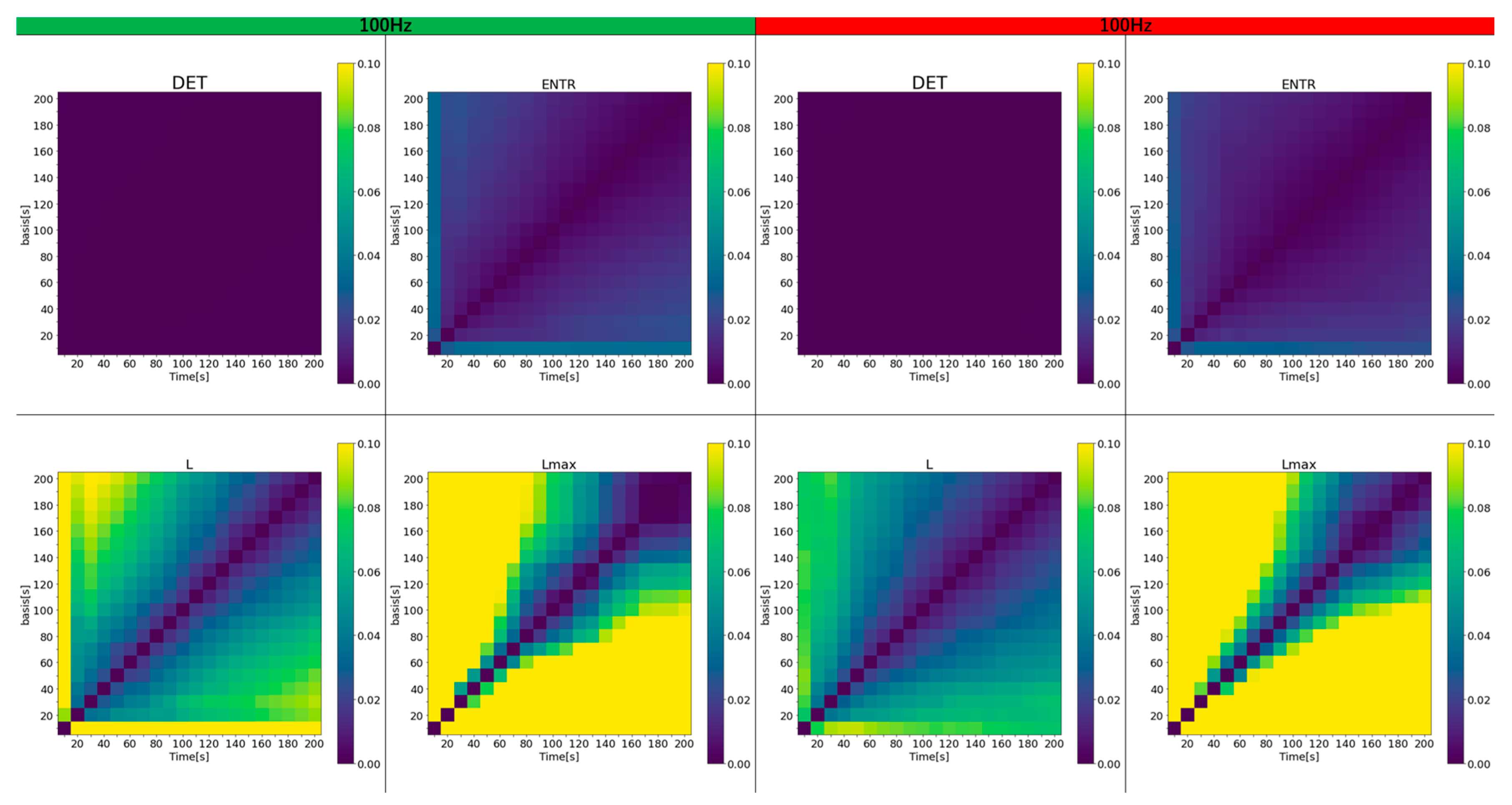
Figure 33.
Change in the average error rate (± 0.5σ) of gPPG (400 Hz) from the standard reference value.
Figure 33.
Change in the average error rate (± 0.5σ) of gPPG (400 Hz) from the standard reference value.
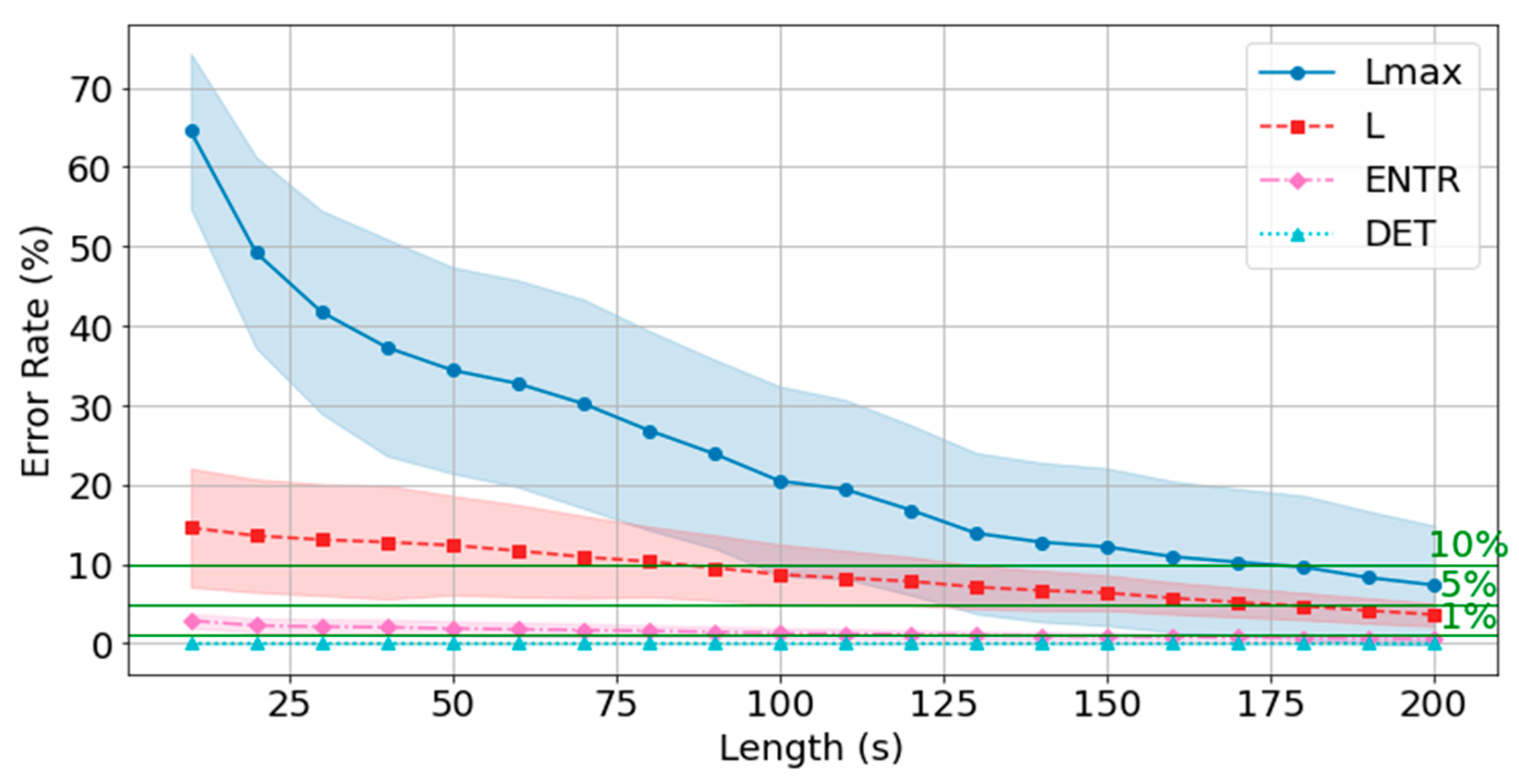
Figure 34.
Change in the average error rate (± 0.5σ) of gPPG (200 Hz) from the standard reference value.
Figure 34.
Change in the average error rate (± 0.5σ) of gPPG (200 Hz) from the standard reference value.
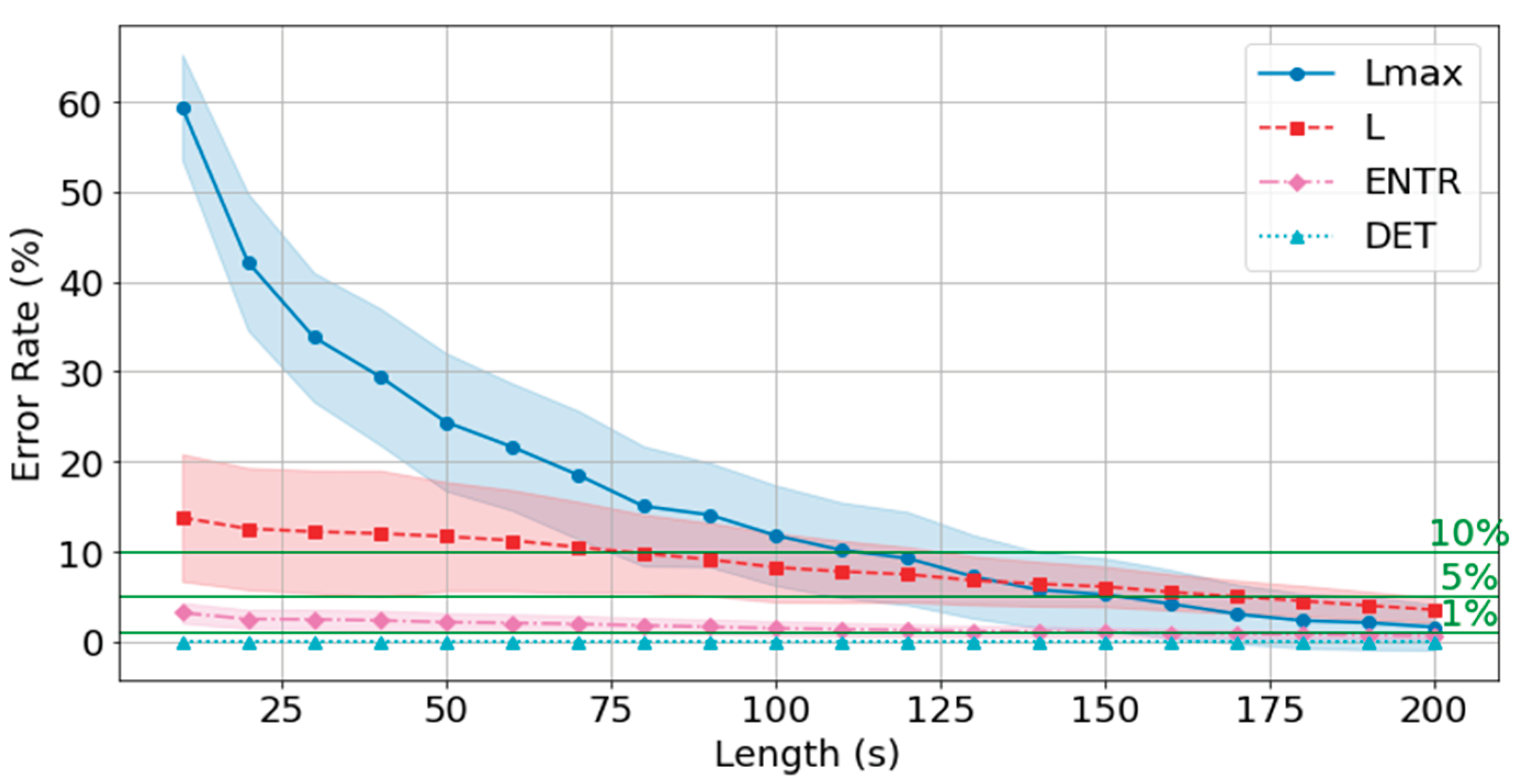
Figure 35.
Change in the average error rate (± 0.5σ) of gPPG (100 Hz) from the standard reference value.
Figure 35.
Change in the average error rate (± 0.5σ) of gPPG (100 Hz) from the standard reference value.
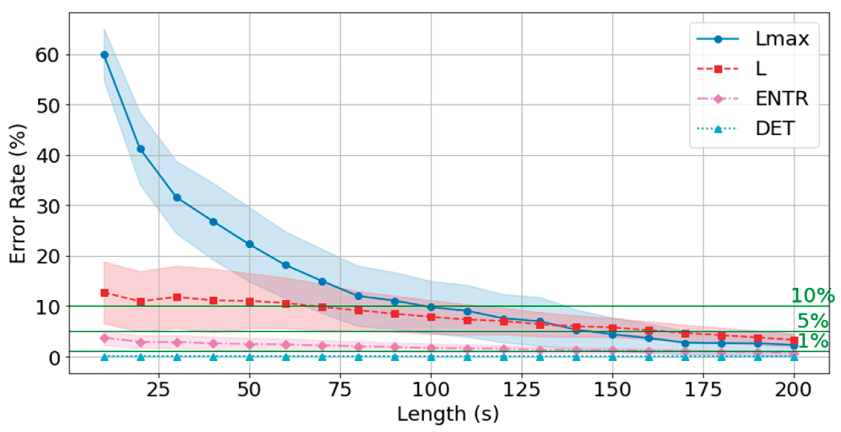
Table 1.
Overview of PPG time series length used in previous studies.
| Topic of Case Study | Time Series Length Used |
| Distinction between normal blood pressure and hypertension [37] | 2.1 s |
| Estimation model of systolic and diastolic blood pressure [35] | 2~3 s |
| Subject authentication method [36] | 7 s |
| Love at first sight impulse detection [43] | 10 s |
| Analgesia depth during anesthesia [44] | 10 s |
| Blood Pressure Estimation [15] | 20 s |
| Mental health assessment [19] | 30 s |
| Correlation with fear/anxiety [45] | 30 s |
| Automatic sleep staging [46] | 30 s |
| Blood sugar estimation [47] | 60 s |
| Early detection of cardiovascular disease [16] | 60 s |
| Automatic Emotion Recognition [48] | 60 s |
| Effects of Mental Stress [21] | 100 s |
| Fatigue Detection [49] | 120 s |
| Estimation of cardiovascular age [17] | 120 s |
| Automatic detection of hypertension [18] | 120 s |
| PPG time series length criteria [42] | 120 s |
| Early detection of depression [22] | 180 s |
| Estimation of blood glucose level [50] | 180 s |
| Effects of changes in gestational age [51] | 180 s |
| Effects of mental illness [20] | 180 s |
| The rPPG dynamics investigation [25] | 300 s |
| The rPPG and gPPG dynamics investigation [11] | 300 s |
| Estimation of blood pressure [39] | 300 s |
| Early hypertension detection [52] | 300 s |
| Effects of tractor noise on the cardiovascular system [53] | 300 s |
| Variation of fatigue during driving [54] | 300 s |
| Comparison between surgical patients and healthy subjects [55] | 300 s |
| Detection of sleep apnea syndrome [56] | 300 s |
Table 2.
Spearman’s rank correlation test results of RQA indices for each frequency (gPPG).
| gPPG | Lmax | L | ENTR | DET |
| 400 Hz vs 200 Hz | 0.78 | 0.98 | 0.98 | 0.98 |
| 400 Hz vs 100 Hz | 0.78 | 0.95 | 0.93 | 0.88 |
| 200 Hz vs 100 Hz | 0.94 | 0.95 | 0.91 | 0.89 |
Table 3.
Spearman’s rank correlation test results of RQA indices for each frequency (rPPG).
| rPPG | Lmax | L | ENTR | DET |
| 400 Hz vs 200 Hz | 0.60 | 0.98 | 0.96 | 0.98 |
| 400 Hz vs 100 Hz | 0.50 | 0.96 | 0.92 | 0.96 |
| 200 Hz vs 100 Hz | 0.94 | 0.97 | 0.94 | 0.96 |
Table 4.
Wilcoxon signed rank test results of RQA indices between gPPG and rPPG.
| Lmax | L | ENTR | DET | |
| 400 Hz | p > 0.05 | p > 0.05 | p > 0.05 | p > 0.05 |
| 200 Hz | p > 0.05 | p > 0.05 | p > 0.05 | p > 0.05 |
| 100 Hz | p < 0.05 | p < 0.05 | p > 0.05 | p > 0.05 |
Table 5.
Summary of the average error rate (%) of gPPG RQA results compared with the reference value.
Table 5.
Summary of the average error rate (%) of gPPG RQA results compared with the reference value.
| time | 400 Hz | 200 Hz | 100 Hz | |||||||||
| Lmax | L | ENTR | DET | Lmax | L | ENTR | DET | Lmax | L | ENTR | DET | |
| 10s | 64.557 | 14.577 | 2.881 | 0.002 | 59.423 | 13.777 | 3.202 | 0.015 | 59.970 | 12.723 | 3.773 | 0.108 |
| 20s | 49.232 | 13.567 | 2.256 | 0.002 | 42.189 | 12.545 | 2.508 | 0.014 | 41.224 | 10.939 | 2.911 | 0.101 |
| 30s | 41.739 | 13.067 | 2.109 | 0.001 | 33.824 | 12.212 | 2.460 | 0.013 | 31.595 | 11.823 | 2.884 | 0.096 |
| 40s | 37.282 | 12.756 | 2.039 | 0.001 | 29.463 | 12.012 | 2.347 | 0.012 | 26.874 | 11.144 | 2.618 | 0.089 |
| 50s | 34.412 | 12.358 | 1.878 | 0.001 | 24.410 | 11.690 | 2.142 | 0.011 | 22.293 | 11.040 | 2.478 | 0.086 |
| 60s | 32.731 | 11.671 | 1.769 | 0.001 | 21.657 | 11.238 | 2.065 | 0.011 | 18.165 | 10.616 | 2.426 | 0.084 |
| 70s | 30.191 | 10.897 | 1.680 | 0.001 | 18.543 | 10.497 | 1.950 | 0.010 | 15.014 | 9.827 | 2.188 | 0.080 |
| 80s | 26.836 | 10.309 | 1.572 | 0.001 | 15.044 | 9.795 | 1.787 | 0.010 | 12.017 | 9.180 | 2.047 | 0.076 |
| 90s | 23.885 | 9.525 | 1.445 | 0.001 | 14.085 | 9.130 | 1.645 | 0.009 | 11.092 | 8.500 | 1.890 | 0.073 |
| 100s | 20.458 | 8.685 | 1.300 | 0.001 | 11.797 | 8.247 | 1.476 | 0.009 | 9.790 | 7.878 | 1.698 | 0.069 |
| 110s | 19.406 | 8.226 | 1.230 | 0.001 | 10.167 | 7.792 | 1.381 | 0.008 | 9.072 | 7.330 | 1.614 | 0.066 |
| 120s | 16.807 | 7.829 | 1.144 | 0.001 | 9.258 | 7.466 | 1.278 | 0.008 | 7.574 | 7.059 | 1.514 | 0.062 |
| 130s | 13.878 | 7.099 | 1.032 | 0.001 | 7.220 | 6.801 | 1.174 | 0.007 | 7.002 | 6.398 | 1.362 | 0.058 |
| 140s | 12.753 | 6.673 | 0.976 | 0.001 | 5.735 | 6.415 | 1.111 | 0.007 | 5.322 | 6.033 | 1.308 | 0.054 |
| 150s | 12.162 | 6.375 | 0.923 | 0.001 | 5.221 | 6.098 | 1.039 | 0.006 | 4.410 | 5.763 | 1.250 | 0.051 |
| 160s | 10.919 | 5.710 | 0.835 | 0.001 | 4.185 | 5.497 | 0.953 | 0.006 | 3.664 | 5.233 | 1.144 | 0.048 |
| 170s | 10.231 | 5.181 | 0.767 | 0.001 | 3.055 | 4.989 | 0.859 | 0.005 | 2.747 | 4.658 | 1.044 | 0.044 |
| 180s | 9.616 | 4.690 | 0.705 | 0.001 | 2.322 | 4.512 | 0.790 | 0.005 | 2.649 | 4.233 | 0.959 | 0.041 |
| 190s | 8.279 | 4.132 | 0.634 | 0.001 | 2.085 | 3.996 | 0.712 | 0.004 | 2.616 | 3.781 | 0.868 | 0.037 |
| 200s | 7.350 | 3.629 | 0.541 | 0.001 | 1.613 | 3.529 | 0.615 | 0.004 | 2.304 | 3.293 | 0.743 | 0.033 |
Disclaimer/Publisher’s Note: The statements, opinions and data contained in all publications are solely those of the individual author(s) and contributor(s) and not of MDPI and/or the editor(s). MDPI and/or the editor(s) disclaim responsibility for any injury to people or property resulting from any ideas, methods, instructions or products referred to in the content. |
© 2025 by the authors. Licensee MDPI, Basel, Switzerland. This article is an open access article distributed under the terms and conditions of the Creative Commons Attribution (CC BY) license (http://creativecommons.org/licenses/by/4.0/).
Copyright: This open access article is published under a Creative Commons CC BY 4.0 license, which permit the free download, distribution, and reuse, provided that the author and preprint are cited in any reuse.


