
Submitted:
02 August 2025
Posted:
04 August 2025
You are already at the latest version
Abstract
This paper presents a comprehensive computational analysis of a real gas turbine, considering the first and second laws of thermodynamics and employing an iterative trial-and-error approach. An equilibrium constant-based combustion model capable of calculating mole fractions of 10 species and applicable to various hydrocarbon fuels has been developed. The model can predict the mole fractions and production rates of pollutants such as NOx, CO, and CO2. In addition, steam injection has been employed in this model to reduce the formation of NOx and other combustion-generated pollutants. This technique lowers the flame temperature and alters the mechanisms of pollutant formation. A comprehensive simulation model was employed in this paper to investigate the impact of steam injection and other key parameters on the performance and emissions of a combined gas cycle. Energy, exergy, economic, and environmental analyses were conducted to provide a comprehensive evaluation of the system. Finally, a modified genetic algorithm is employed to optimize a multi-objective function considering total cost rate, CO2 index, and second law efficiency. The results of the developed combustion model have been validated against CEA and GASEQ software, demonstrating a maximum average error of only 0.5027% for 10 species. As a result of the multi-objective optimization, a three-dimensional Pareto front is obtained, indicating a maximum achievable exergy efficiency of 0.4058%, a minimum total cost rate of $1471.2 per hour, and a CO2 index of 0.5075 kg/kWh. The distribution of the primary decision variables reveals the optimal range for these variables where Pareto optimal points are obtained. Based on the scatter analysis, the optimal steam injection mass flow rate was determined to be 26.9 kg/s (corresponding to 10.63% of the total air mass flow rate). This optimal value simultaneously optimizes the system's performance, economic, and environmental indicators.
Keywords:
energy
; exergy
; exergoeconomic
; gas turbine
; steam injection
; multi-objective optimization
; hazardous emissions
1. Introduction
Gas turbines are essential equipment in the oil and gas industry, used for power generation and driving compressors, pumps, generators, and more. In gas pipeline compressor stations, they are employed to compress pipeline gas and overcome pressure drops. Improving the efficiency of gas turbines would significantly contribute to reducing energy consumption in the gas transmission industry. Various methods have been widely used to enhance gas turbine performance, including inlet air cooling using evaporative, absorption, or mechanical refrigeration, recuperation, water injection into the recuperator inlet air, combined cycles with or without reheat, steam or water injection into the combustion chamber inlet air, and flue gas heat recovery [1,2]. The selection of an optimal method to enhance gas turbine performance is influenced by a multitude of factors, including turbine application, environmental conditions, and operational parameters. The specific process, equipment, design, and age of the turbine, as well as ambient conditions, significantly impact the choice of an effective method. Given the pressing need to conserve fossil fuels and mitigate environmental impacts, engineers are continually exploring advanced technologies and optimization techniques to improve the efficiency of energy generation systems [3].
One approach to enhancing power plant efficiency involves upgrading the materials used in their construction. Employing materials with superior high-temperature resistance can lead to improved efficiency and extended equipment lifespan. Furthermore, integrating older power plants with newer technologies to create combined cycles, coupled with advanced carbon capture and storage methods, can significantly reduce pollutant emissions. However, energy engineers face complex challenges. Selecting the appropriate technology, considering climate change, and addressing socioeconomic factors are crucial considerations in the design and construction of energy systems. An ideal energy system should exhibit high efficiency, low construction and maintenance costs, flexibility in fuel utilization, a short construction timeline, minimal environmental impact, and high reliability [4,5].
A deep understanding of energy conversion processes and factors influencing energy losses is crucial for optimizing energy systems. Furthermore, adopting a systems-based approach in the design and operation of these systems is essential to reduce environmental pollution and enhance energy sustainability. Consequently, energy system optimization has emerged as one of the most significant engineering challenges of our time.
Several researchers have conducted exergoeconomic and thermodynamic analyses of integrated gas turbine-based systems. Ahmadi et al. [6] optimized a CHP system using a multi-objective approach based on the exergy concept. They conducted sensitivity analyses to investigate the impact of changes in design parameters on the overall system performance from energy and exergy perspectives. The primary objectives of this research were to improve system performance in terms of efficiency, fuel consumption, energy losses, production costs, profitability, and environmental pollution reduction. Sahin and Ali [7] investigated the optimized performance of a combined cycle system based on the Carnot cycle under steady-state conditions, considering efficiency reduction factors. They analytically calculated the maximum power and efficiency of this system and evaluated the impact of various factors on the output power. Despite the significance of exergoeconomic and thermodynamic analysis in evaluating power generation systems, these methods alone cannot accurately determine optimal design parameters. Sahoo [8], in their research, employed evolutionary optimization methods for a comprehensive economic and energy analysis of a CHP system. By applying thermodynamic and economic principles, Sahoo achieved an optimal configuration for this system, resulting in a 9.9% reduction in electricity production costs and overall system costs compared to the initial state.
In another study, Ahmadi and Dincer [9] investigated the performance of dual-pressure combined cycle power plants having supplementary firing. By incorporating exergy destruction costs into the optimization objective function, the researchers utilized a genetic algorithm to find the optimal system settings. Mozafari et al. [10] conducted comprehensive energy, cost, and environmental analyses to optimize microturbines. This research was conducted using various fuels, and the results indicated that the type of fuel had a negligible impact on the optimization objectives, and the trends of thermodynamic efficiency and overall system costs were independent of the fuel type. Suresh et al. [11], through a comprehensive study of advanced coal-fired power plants, examined various energy, exergy, and environmental aspects. While this study thoroughly evaluated the environmental impacts of pollutant emissions such as carbon dioxide, sulfur oxides, and nitrogen oxides, power cycle optimization was not considered. The results indicated that under Indian climatic conditions and using high-ash coal, the maximum achievable energy efficiency in these power plants is approximately 42.3%. Sahat et al. [12] conducted a comprehensive review investigating the effects of steam addition on combustion processes. The study aimed to analyze previous research in this field. Researchers categorized existing studies based on case studies, methodologies, design criteria, and performance parameters. Results indicated that a significant benefit of steam injection into combustion processes is a substantial reduction in NOx emissions. This advantage justifies the widespread application of this technique in various industries. Furthermore, research suggests that other pollutants either remained unchanged or experienced negligible changes under the influence of this method.
In this paper, the performance of a combined gas cycle has been thoroughly investigated using thermodynamic modeling, exergy analysis, and multi-objective optimization. Thermodynamic modeling in this paper has been presented using a trial-and-error method and iterative loops, considering thermodynamic laws, and it has a very high accuracy. Moreover, previous studies have used empirical formulas or CFD methods to calculate NO and CO, each of which has its own advantages and disadvantages. For example, using empirical methods can introduce significant errors in calculations, and CFD methods are also time-consuming and expensive. In this research, a comprehensive combustion modeling method has been used, and the mole fraction of 10 combustion species has been calculated. Finally, it is coupled with the stated thermodynamic algorithm. Additionally, the CoolProp module in MATLAB software has been used to calculate thermodynamic properties in this paper [13].
In the presented combustion model, the amount of steam or water fraction can be easily calculated and added to the combustion process, and the effects of adding steam to the combustion chamber can be calculated using the energy conservation law. Sensitivity analysis has also been performed for important gas turbine parameters, including pressure ratio, fuel stoichiometric ratio, and the amount of injected steam under various conditions. Finally, using a modified genetic algorithm, three objective functions have been considered: exergetic efficiency, total system cost rate, and CO2 emission rate. In this paper, a comprehensive simulation model has been developed to enhance the efficiency and mitigate the environmental impacts of gas turbine cycles. By incorporating the molar fraction of water into the combustion equation, this innovative approach investigates the effects of steam injection. The decision variables include the compressor pressure ratio, compressor and turbine isentropic efficiency, combustion chamber efficiency, fuel stoichiometric ratio, and steam mass flow rate. Consequently, this research aims to investigate the following objectives:
- A mathematical framework is developed to simulate the gas turbine cycle, considering the principles of energy and entropy conservation. Iterative algorithms are employed to solve the governing equations.
- A comprehensive analysis of energy losses in a gas turbine cycle is conducted by calculating exergetic efficiency and identifying the major components contributing to exergy destruction.
- Developing a model to solve combustion equations with detailed NO and CO emissions using equilibrium constants
- Developing a model considering the effects of steam injection on CO2 emissions, efficiency, and total cost rate
- Sensitivity analysis of important gas turbine parameters
- Multi-objective optimization of cost, efficiency, and CO2 emissions
- Presenting a three-dimensional Pareto front as a result of multi-objective optimization using a modified genetic algorithm
- Showing the distribution of scatter plots to determine the optimal value for decision variables
- Presenting an ideal point in multi-objective optimization, including the ideal point of cost, efficiency, and CO2 emissions.
2. Solution Method and Governing Equations
Figure 1 shows a simplified schematic of a gas turbine cycle. As shown, a gas turbine consists of three main parts. These components are the air compressor, combustion chamber, and turbine. Ambient air (point 1) first enters the compressor and its pressure is increased by the compressor (point 2). Then, air and fuel enter the combustion chamber and are burned (point 3). The combustion gas, which has a high temperature and pressure, passes through the turbine and drives it, and the rotational force produced by the turbine is transferred to the generator or other equipment such as pumps and compressors. After passing through the turbine, the pressure of the combustion gas reaches a pressure close to the ambient pressure and enters the atmosphere (point 4) [14,15].
2.1. Energy Analysis
The major part of energy modeling is applying mass and energy balance equations. In this section, the thermodynamic relations governing the gas turbine are analyzed [16].
- Free Stream: Temperature and static pressure are two crucial factors in analyzing the behavior of fluid flow in the Earth’s atmosphere. These parameters undergo significant changes with increasing altitude above sea level. Up to an altitude of approximately 11 kilometers, specific mathematical relationships, expressed as Equations (1) and (2), describe the variation of temperature and pressure with altitude.
The enthalpy and entropy of the air entering the compressor are considered according to equations (3) and (4) below [17].
Compressor: Air enters the compressor and is compressed in a polytropic process. The actual work consumed by the compressor during the compression process is calculated using equation (5).
The isentropic efficiency of the compressor is also defined as the ratio of the isentropic work to the actual work of the compressor and is determined by equation (6).
In an isentropic process, . Additionally, for calculating enthalpy and entropy, the following equations are used (equations (7) and (8)) [2]:
Combustion Chamber: The heat balance equation in the combustion chamber is expressed as equation (9) [18].
where is the enthalpy at the outlet of the combustion chamber. Additionally, and is the efficiency of the combustion chamber. The outlet pressure is also obtained as follows (equation (10)):
where is the pressure drop across the combustion chamber. In equation (9), the outlet enthalpy and are obtained by solving the combustion equations.
- Combustion Equation: The primary equation in the combustion chamber is considered based on the chemical equation for various hydrocarbon fuels as equation (11) [19].
By balancing the species, the following system of equations (equation (12)) is obtained:
Where, is the mole fraction of each species and is calculated as follows (equation (13)):
In the system of equations (12), the values of , , and are known. This system of equations includes 11 unknowns. To solve the above equation and obtain the values of n and , the following auxiliary equations and equilibrium constants are required [20].
In addition, the equilibrium constant associated with each equation can be obtained from the polynomial coefficients presented below (Equation (15)) [20]:
Table 1 shows the values of the coefficients required to calculate the equilibrium constants in Equation (15).
In order to linearize the system of equations (12), the following constants were used (Equation (16)).
Considering the defined constants and substituting them into the system of equations (Equation (12)), the atomic species balance equations are rewritten as follows. Also, the sum of the mole fractions of the combustion products is equal to 1. Therefore, the new system of equations is written as Equation (17).
Additionally, the auxiliary equations are rewritten as follows, so that they can be used in the system of equations (17) (Equation (18)).
By substituting the aforementioned relations into the system of equations (17), the final system of equations (19) is obtained. The following equations consist of 4 equations and 5 unknowns ( and ). Therefore, the energy balance equation between the reactants and combustion products must also be added to the following equations.
The system of equations (19) can be expressed as the following relation (Equation (20)).
The system of equations shown in Equation (20) can be solved using the Newton-Raphson iterative method. If the solution vector of Equation (20) , is denoted as the left-hand side of the equation , for a first-guess solution vector close to , is expanded using a Taylor series, and second-order and higher partial derivatives are neglected. Thus, we have:
In Equation (21), .
Equation (21) can be rewritten in matrix form as , where matrix A is actually the Jacobian matrix of the system, as defined in equation (22) [22].
To solve this system of equations, the Gaussian elimination method, as detailed in equation (23), was employed. The resulting vector from this method was then used as the initial point for optimizing the problem’s initial vector [22].
where k is the number of iterations. The iterative process continues until the value of is within a predefined tolerance (ε=0.001) of the target value. The maximum number of iterations is limited to 20. It is worth noting that, in addition to the iterative formula, the choice of the initial value significantly impacts the convergence rate and success of the optimization process. The initial solution vector , were determined by modeling incomplete combustion of fuel at temperatures below 1000 Kelvin.
Initial Estimation of Mole Fractions: To obtain the mole fraction values, it is necessary to initially estimate the four mole fractions . Therefore, the combustion equation is considered as follows (Equation (24)):
By writing balance equations for each species, the system of equations (25) can be obtained as follows:
To simplify the equations, the following four constants are defined (Equation (26)).
Using the two auxiliary equations) ( and substituting them into the above equations, a relationship in terms of the variable is obtained as follows (Equation(27)).
By guessing the value of and using the energy balance equation, the only unknown in the above equation is N. The value of N can also be obtained by considering the following two cases.
- Case 1: In fuel-lean combustion mixtures (ϕ < 1), due to the deficiency of oxygen, we assume that carbon monoxide (CO) and hydrogen (H2) are completely consumed in the reaction and are not present in the combustion products. Consequently, by setting the number of moles of CO and H2 to zero (i.e.), the number of unknowns in the mass balance equations is reduced, simplifying the solution of the equation system.
- Case 2: In fuel-rich combustion mixtures (ϕ > 1), due to the excess of fuel relative to air, all available oxygen is consumed, leaving no residual oxygen in the combustion products (i.e.
- ). To accurately determine the composition of the incomplete combustion products under these conditions, in addition to atomic balance equations, it is necessary to consider the equilibrium reaction between the products CO2, H2O, CO, and H2. This equilibrium reaction, also known as the water-gas reaction, is represented by equation (28).
The numerical value of the equilibrium constant for the water-gas shift reaction is denoted by KT and is presented in equation (29).
The equilibrium constant equation for , is obtained using Equation (30).
By writing balance equations for each species, the final equations for both cases can be summarized in the following table.
Also, the coefficients a, b, and c are obtained as follows (Equation (32)).
By calculating the values of N and using the relation , the value of N is obtained. Therefore, by calculating the value of N to solve Equation (27), it is assumed that the initial mole fraction of the combustion product is 100%, i.e., . This clearly causes to be greater than 0. Then, Equation (33) is used to iterate until becomes less than 0. At this point, will be close to its exact value.
To achieve greater accuracy in the calculations, the values obtained from the initial iterative method can be used as an initial guess in the Newton-Raphson method. This numerical method, whose formula is presented in equation (34), allows us to obtain a more accurate and faster solution.
When the absolute value ratio of to is less than 0.001, it can be considered that the exact value of has been successfully obtained. The initial values of the mole fractions, and can be obtained using Equation (25) [19].
Thermodynamic Property Calculations: Accurate simulation of gas turbine engine performance necessitates precise modeling of the thermal properties of combustion products. By examining and comparing various models for specific heat capacity at constant pressure (cp) and volume (cv), it was found that increasing the complexity of these models leads to a decrease in the calculated thermal efficiency of a standard air dual cycle and a closer convergence of results with the actual thermal efficiency of diesel engines.
Many studies have simplified the thermal properties of combustion products by assuming a linear relationship with temperature, neglecting the effects of pressure and fuel-air ratio. For instance, Lamas’ model considered only five primary combustion product components (O2, N2, CO2, H2O, and SO2) and disregarded the variation of thermal properties with pressure. These simplifications are made despite the fact that complex chemical reactions occur at high combustion chamber temperatures, leading to a significant increase in the number of combustion product components. Furthermore, the concentration of these components is strongly dependent on temperature and fuel-air ratio. Consequently, neglecting these complexities compromises the accuracy of simulation models [22,23].
In many studies, for the sake of computational simplicity, the constituent gases of a combustion mixture are assumed to behave as ideal gases. The thermodynamic properties of these gases are typically obtained from tables or empirical correlations. In this study, we have adopted a comprehensive data-based approach developed by Gordon and McBride. This method relies on fitting NASA polynomials to experimental data. Utilizing these polynomials and considering the mole fractions of each component in the mixture, determined through chemical equilibrium calculations, we can calculate the thermodynamic properties of the mixture using the Gibbs-Dalton law [24]. Equation (35) presents the relationships for calculating molar mass, molar specific enthalpy, molar internal energy, and molar entropy [22].
While individual components of a gas mixture can be considered as ideal gases, the overall behavior of the gas mixture does not necessarily follow the ideal gas laws. For instance, the specific internal energy of a gas mixture is not solely a function of temperature. To more accurately describe the behavior of such gases, modifications to the ideal gas equation of state are required, such as adjusting the universal gas constant (as seen in Equation (36)) [22].
Specific heat capacity at constant pressure is defined as the partial derivative of internal energy with respect to temperature under isobaric conditions. This quantity represents a system’s ability to absorb heat and increase its temperature at constant pressure, and is expressed by the differential equation (37).
Based on Equation (36), the specific enthalpy of the gas mixture can be expressed as follows (Equation (38)):
By substituting the relationships, the specific heat capacity is calculated using Equation (39).
The second and third terms on the right-hand side of the above equation represent the kinetic effects of dissociation reactions on the molecular composition of combustion products at elevated temperatures. However, at lower temperature regimes where dissociation reactions are less significant, equation (40) can be approximated by a simpler model.
To determine the specific heat capacity at constant pressure () as defined by equation (40), it is necessary to calculate the partial derivatives of the mole fractions () of each chemical species in the gas mixture with respect to temperature. This can be achieved by differentiating the chemical equilibrium equation (20) with respect to temperature, resulting in a set of partial differential equations for components , , and (equation (41)).
By calculating the derivatives expressed in the equation, the following matrix is finally formed, and the method of solving this equation is similar to Equation (20) (Equation (42)).
To obtain the derivatives of functions with respect to pressure, a process similar to calculating the derivative with respect to temperature is performed, and the solution method is also similar to the previous method (Equation (43)).
Also, the enthalpy, specific heat capacity, and entropy of each component are calculated as follows (Equations (44-47)) [22].
The coefficients presented in the above equations are extracted from reference [25] for temperatures ranging from 300 to 1000 Kelvin and from 1000 to 3000 Kelvin. Therefore, the specific volume is equal to (Equation (48)):
The derivative of specific volume with respect to temperature at constant pressure (Equation (49)):
The derivative of specific volume with respect to pressure at constant temperature (Equation (50)) [22]:
Steam Injection into the Combustion Chamber: Steam injection into the combustion chamber of gas turbines is an effective method for reducing combustion-generated pollutants, especially nitrogen oxides (NOx), and improving turbine performance. Therefore, this paper aims to complete the described algorithm and to include the effects of steam injection on the combustion process in the developed model. With steam injection into the combustion chamber, the combustion equation is rewritten as Equation (51).
The amount of , the percentage of steam injection into the combustion chamber, is obtained using Equation (52) [26].
Therefore, to simulate the effects of steam injection into the combustion chamber, the value of must be specified. In this case, the species balance equation (Equation 12) is modified considering the value of .
Energy Balance Equation: The energy balance equation for the control volume of the combustion chamber is obtained according to Equation (53) [27].
Also, considering the effects of steam injection, we have (Equation 54):
In this relation, and it is assumed that the amount of heat transferred from the combustion chamber is equal to 2% of the lower heating value of the fuel, and its value is calculated using Equation (55) [28].
Also, is the molar enthalpy of the fuel at the inlet fuel temperature. The inlet fuel temperature is considered to be the same as the ambient temperature. According to the problem assumptions, the inlet air and combustion products are considered as an ideal gas mixture. Therefore, and are calculated using the following relations. is also the enthalpy of steam at the desired temperature (Equations (57-58)).
Finally, a system of equations with 5 equations and 5 unknowns is obtained. Solving the above equations ends with assuming an initial value for or and establishing the energy balance condition.
Turbine: The work produced by the turbine during the isentropic expansion process is obtained using Equation (59):
Isentropic efficiency of a turbine is a measure of turbine performance, indicating how closely the actual turbine operation approaches an ideal, reversible process. It is defined as the ratio of the actual work output of the turbine to the ideal work output under isentropic conditions (i.e., without energy losses due to friction or heat transfer). This efficiency is calculated using Equation (60).
In the isentropic process in the turbine, .
Finally, the energy efficiency is obtained by Equation (61) [2].
Figure 2 shows the algorithm for solving the energy equations.
2.2. Exergy Analysis
Exergy represents the maximum work a system can produce when it reaches equilibrium with its surroundings. This quantity depends on the internal factors of the system and the environmental conditions. Exergy analysis, by combining the second law of thermodynamics with the principles of mass and energy conservation, enables the identification and localization of energy losses. By using this analysis, the system can be optimized to minimize energy losses. The exergy of a system consists of various components such as kinetic, potential, chemical, and thermal energy, all of which are included in the exergy balance equation (Equation (62)). [29].
The amount of exergy destruction () in the above equation is of great importance, as this quantity indicates the amount of potential lost by a component or the entire system to perform useful work. In fact, exergy destruction indicates how much of the system’s initial exergy is irreversibly converted to thermal energy of the environment due to thermodynamic limitations and other unavoidable factors, reducing the system’s ability to perform useful work. Therefore, Equation (63) represents the exergy balance in each component of the system.
The exergy of each inlet and outlet stream of the system consists of two main components: physical exergy and economic availability. Physical exergy represents the inherent ability of a stream to perform mechanical work, resulting from differences in physical parameters such as pressure, temperature, and elevation relative to the surroundings. On the other hand, economic exergy refers to the economic value of a stream due to its specific chemical composition or location. The formulas for calculating these two components are presented below (Equations (64-66)) [29].
The exergy efficiency and exergy destruction of all components are presented in Table 3.
2.3. Economic Analysis
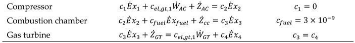
In the process of developing economic balance equations for gas turbine equipment, the economic value of each component must first be determined. The cost incurred in each component is known as exergy destruction cost and the primary objective of this analysis is to minimize this cost. By applying the principle of cost balance to component k, the relationship between the total costs associated with exergy outflow streams and the total costs of exergy inflow streams, along with fixed costs (including initial investment and operational and maintenance costs), can be established. The sum of fixed costs is denoted by Z. Based on this principle, the cost rates of the system’s exergy inflow and outflow streams and ultimately, the unit cost of exergy products can be calculated. The equation for component k is presented as Equation (67) [30].
When analyzing a system where the exergy outflow from a component (Ne) is unknown, an equation deficiency arises. To address this issue, the principles of F and P within the SPECO framework are employed to introduce a sufficient number of auxiliary equations to the system. By developing these auxiliary equations for all components of the gas cycle system, a comprehensive system of equations is obtained, as presented in Table 4. Solving this system of equations enables the accurate calculation of all desired variables [30].
In the aforementioned equation, the parameter represents the annual operating cost of each component in the system and is calculated using Equation 68. To calculate , initial data such as the initial investment cost (presented in Table 5, the capital recovery factor (CRF), the maintenance factor (), and the annual operating hours of the system (N) are required. By utilizing these parameters and referring to Equation )68(, the annual operating cost of each component can be accurately determined.
By solving the system of equations, the cost of unknown system streams is obtained. The desired equations are solved using the matrix formation method below (Equation (68)).
2.4. Optimization
Initially, the objective functions are defined. In this paper, exergy efficiency, CO2 index, and total system cost are considered as the objective functions. Equation (69) is employed to determine the exergetic efficiency [31].
In this equation, corresponds to the chemical exergy coefficient of methane gas. Also, for the total system cost, we have (Equation )70():
By applying energy and cost balances to all components of the system, the costs associated with each component are calculated. Based on Equation (71), the cost of exergy destruction () is also determined.
In the above equation, represents the exergy destruction rate in component k, and denotes the unit cost of fuel consumed in that component. The unit cost of natural gas fuel is also calculated using Equation (72).
The environmental cost due to the emission of CO2, CO, and NO pollutants is also calculated using Equation (73).
Where the values of , , and are considered to be 0.024, 0.02086, and 6.853 respectively. Finally, the CO2 index is also determined using Equation (74) [31].
Accordingly, using the algorithm shown in Figure 3, a multi-objective optimization is performed with the aim of maximizing exergy efficiency and simultaneously minimizing the total cost rate and CO2 index.
3. Results and Discussion
In this section, the results of the combustion model presented in this research are first compared with commercial software such as CEA and GASEQ for validation. In the next section, the results are compared with the reference results of an industrial gas turbine [32] to ensure the accuracy of the algorithm for gas turbine analysis. Subsequently, the results of various assessments, including energy, exergy, economic, and environmental evaluations of the proposed model, are presented. Following this, a parametric study is conducted to investigate the sensitivity of the gas turbine’s performance to variations in key parameters. Finally, the results of the multi-objective optimization, using Pareto frontier analysis and the distribution of decision variables, are presented to determine the optimal operational range [33].
3.1. Model Validation
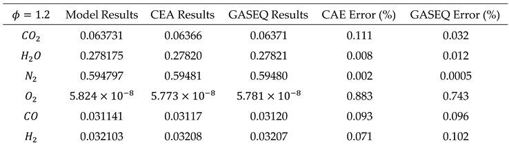
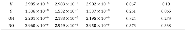
To validate the results obtained from the combustion model, a comparison was made between the model results and the commercial software CEA and GASEQ. Methane was considered as the fuel, and the composition of the air was assumed to be 0.79% nitrogen and 21% oxygen. Additionally, the steam injection rate into the combustion chamber was considered to be 10% in both cases.
As evident from the results in Table 6 and Table 7, the presented model demonstrates a high degree of accuracy in calculating the mole fraction of combustion products. Therefore, the presented model can be used to calculate combustion species in gas turbine combustion chambers.
.
.
3.2. Energy Model Validation
Following the validation of the combustion model, we proceed to validate the gas turbine performance modeling. This section presents the validation of the proposed model for a Siemens V94.2 gas turbine. Table 8 compares the gas turbine cycle validation against the reference study data [32] for the case without steam injection and an air mass flow rate of 490 kg/s. The results in Table 7 indicate that the proposed model exhibits sufficient accuracy for gas turbine performance analysis.
3.3. Parametric Study
Through a sensitivity analysis of critical parameters, the performance of the gas turbine was assessed under both base and steam injection conditions. Finally, considering the multi-objective Pareto front and the distribution of each parameter, the optimal range of each decision variable is presented. To examine the results of the proposed model, a gas turbine (GE 9E model) has been used. The specifications of the gas turbine are given in Table 9 [14].
Exergy Analysis: Exergetic evaluation reveals that while energy efficiency solely focuses on the quantity of input and output energy, exergy efficiency serves as a more comprehensive metric, considering both the quality of energy and its potential to perform useful work. The results of the exergy analysis demonstrate that while the gas turbine exhibits a high exergetic efficiency of 94.64% and the air compressor operates at 93.32%, the combustion chamber is identified as the system’s bottleneck with an exergetic efficiency of only 74.44%, indicating significant potential for improvement. Figure 4a corroborates this finding, showing that the combustion chamber experiences the most exergy destruction, accounting for 85.94% of the total exergy destruction within the system. These results underscore the importance of optimizing the combustion process to reduce energy losses and enhance overall system efficiency.
Two parameters that significantly impact the performance of gas turbines are the compressor pressure ratio and the fuel stoichiometric ratio. The effect of these two parameters on exergy efficiency, CO2 emissions and total cost rate is shown in Figure 5, Figure 6 and Figure 7. In the first case, the analysis is conducted without considering the effects of steam injection.
Figure 5 illustrates the impact of compressor pressure ratio and fuel stoichiometric ratio on the gas cycle unit efficiency. When the pressure ratio is constant, increasing the fuel stoichiometric ratio leads to an increase in the overall exergy efficiency of the unit. Similarly, at a constant fuel stoichiometric ratio, increasing the compressor pressure ratio enhances the gas turbine efficiency. Generally, with increasing compressor pressure ratio, exergy efficiency typically increases initially, reaches a maximum, and then decreases. This is due to the increased work output of the turbine with increasing pressure ratio, but on the other hand, the increased work required for the compressor also reduces efficiency. Figure 6 shows that, at a constant pressure ratio or fuel stoichiometric ratio, increasing the other variable parameter leads to an increase in the total cost rate, but the impact of the fuel stoichiometric ratio on increasing the total cost rate is more significant. Generally, increasing the compressor pressure ratio usually leads to an increase in system efficiency. This can result in reduced fuel consumption and consequently lower fuel costs. However, with increasing pressure ratio, initial investment costs for equipment, as well as maintenance costs, may increase. Therefore, a balance between increasing efficiency and related costs is necessary. Additionally, selecting an appropriate stoichiometric ratio contributes to increased combustion efficiency and reduced emissions. This can lead to lower costs associated with exhaust gas treatment and environmental fines. Very low or high ratios can result in incomplete combustion, which will incur additional costs for gas treatment and increased fuel consumption. In Figure 7, at a constant fuel stoichiometric ratio, increasing the compressor pressure ratio decreases the CO2 emission rate due to the increased net work output of the turbine. Furthermore, increasing the compressor pressure ratio increases the temperature and pressure of the air entering the combustion chamber. This leads to increased combustion efficiency and reduced fuel consumption. Consequently, the CO2 emission rate decreases. Although increasing the compressor pressure ratio increases the temperature of the gases exiting the combustion chamber, this temperature increase is a smaller percentage compared to the increase in the net work output of the turbine. Therefore, increasing the compressor pressure ratio at a constant stoichiometric ratio results in a decrease in the CO2 emission rate.
Steam Injection into the Combustion Chamber: To control the turbine outlet temperature, a significant amount of excess air is required. On the other hand, increasing the inlet air flow rate increases the power consumption of the compressor. If, instead of excess air, a suitable amount of steam is injected into the combustion chamber to control the inlet temperature to the turbine, the work consumed by the compressor decreases due to the reduced air flow rate, and the steam flow in the turbine compensates for the reduced air flow and the reduced work produced by the turbine, resulting in an overall increase in net work output. Therefore, in this paper, the effect of steam injection into the combustion chamber on increasing efficiency and important turbine parameters is investigated. In this method, the liquid water pressure is first increased to the combustion chamber pressure by a pump and then converted to steam by the exhaust gases from the power plant in a heat exchanger, and then injected into the combustion chamber. Steam injection occurs after the fuel and air combustion process and in the elbow and exit region of the combustion products. It should be noted that with this method, the increase in input work by the pump can be neglected compared to the significant decrease in compressor input work. Therefore, this section examines the impact of steam injection under various conditions.
Effects of Steam Injection at Different Compressor Pressure Ratios: Figure 8 illustrates the impact of compressor pressure ratio and steam injection rate on exergy efficiency. By keeping either the pressure ratio or injection rate constant and increasing the corresponding parameter, the efficiency increases. However, the effect of adding steam flow rate on increasing efficiency is greater compared to the compressor pressure ratio. Figure 9 shows that at a constant pressure ratio, increasing the injection rate decreases the total cost rate. This is because the cost associated with environmental pollutants decreases. However, at a constant injection rate, increasing the compressor pressure ratio increases the total cost rate. This is because the value of ZAC increases with increasing pressure ratio. Figure 10 shows that by increasing the injection rate and compressor pressure ratio, CO2 emissions decrease. Moreover, the percentage reduction in CO2 due to the addition of steam is significantly higher than that of increasing the compressor pressure ratio. Therefore, it can be concluded that the use of steam injection is essential to increase energy and exergy efficiency and reduce CO2 emissions. This is because the compressor pressure ratio can only be increased to a certain extent due to design limitations, and this increase alone cannot replace the addition of steam to the combustion chamber. It has been shown that CO2 emissions and exergy efficiency are aligned and there is no contradiction. This is mainly because CO2 in the exhaust gases is primarily caused by the combustion of carbon in the fuel. When the load is constant, the higher the efficiency, the less natural gas is required, and consequently, CO2 emissions are also reduced.
Effects of Steam Injection and Different Fuel Stoichiometric Ratios: Figure 11 demonstrates that increasing both the steam injection rate and the fuel stoichiometric ratio leads to an increase in exergy efficiency, however, the impact of increasing steam injection on enhancing efficiency is significantly greater than that of the fuel stoichiometric ratio. Figure 12 indicates that increasing the fuel stoichiometric ratio at a constant injection rate results in a substantial increase in the total cost rate, while at a constant stoichiometric ratio, increasing the injection rate does not significantly decrease the total cost rate. It can be concluded that the effects of the fuel stoichiometric ratio on the total cost rate are more significant compared to the injection rate. Figure 13 shows that increasing both the fuel stoichiometric ratio and the injection rate decreases CO2 emissions, but the impact of increasing the steam injection rate on reducing CO2 emissions is significantly greater than that of increasing the stoichiometric ratio. In this case, it is also shown that CO2 emissions and exergy efficiency are aligned.
Effects of Steam Injection on NO and CO Emissions: Figure 14 and Figure 15 demonstrate that increasing the steam injection rate leads to a decrease in combustion temperature and consequently a reduction in equilibrium constants and pollutant emissions. Adding 30 kg of steam to the combustion chamber results in a 5% decrease in TIT. In other words, for each kilogram of injected steam, TIT decreases by 0.1683%. Additionally, adding 30 kilograms of steam to the combustion chamber results in a 26.05% reduction in NO production and a 67.8% reduction in CO production. That is, for each kilogram of injected steam, the amounts of NO and CO decrease by 0.87% and 2.26%, respectively.
3.4. Multi-Objective Optimization Results
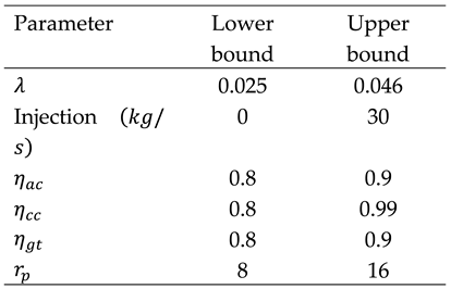
Table 10 presents the decision variables along with their corresponding upper and lower bounds. These bounds are imposed due to availability or metallurgical constraints.
The results of the multi-objective optimization Achieved from the GA are presented as a Pareto front in Figure 16. This front shows the relationship between exergy efficiency, CO2 index and total cost rate. As expected, due to the multi-objective nature of the problem, instead of a single optimal point, a set of optimal points (Pareto front) is obtained. In this set, increasing energy efficiency is accompanied by a decrease in pollutant emissions. The ideal point, where the highest energy efficiency and the lowest cost and pollution coexist, is shown in the figure. The values of this point for the maximum achievable exergy efficiency are 0.4058%, the minimum total cost rate is 1471.2 $/h, and the CO2 index is 0.5075 kg/kWh.
Figure 17, Figure 18 and Figure 19 illustrate the distribution of compressor efficiency, combustion chamber efficiency, turbine efficiency, injected steam mass flow rate, compressor pressure ratio, and stoichiometric fuel ratio, respectively. By analyzing the points obtained from the GA and plotting the Pareto front, the optimal range for each decision variable can be identified. Figure (17) shows that the optimal value of compressor efficiency is 0.865 and the optimal value of combustion chamber efficiency is 0.975. Additionally, Figure (18-a) shows that the optimal turbine efficiency is distributed in the range of 0.85 to 0.89, and based on the Pareto front distribution, a value of 0.891 can be selected as its optimal value. Figure (18-b) indicates that the optimal value of the injected mass flow rate is 26.9 kg/s. Moreover, Figure (19-a) shows that the optimal value of the stoichiometric fuel ratio is 0.259. However, Figure (19-b) indicates that the optimal pressure ratio for the compressor is distributed in the range of 8.5 to 12.5, and based on the Pareto front distribution, a value of 12.35 can be selected as its optimal value.
4. Conclusions
In this paper, a model based on iterative loops was introduced using computer code and the first and second laws of thermodynamics to calculate the thermodynamic characteristics and performance of a gas cycle. As shown, in this method, with the given turbine inlet temperature (TIT) or fuel stoichiometric ratio and using a trial-and-error method, the thermodynamic parameters of the cycle can be calculated. The validation of the stated model showed that this model has an acceptable accuracy. Also, considering the importance of environmental pollutant emissions, a combustion model was developed using equilibrium constants, and the mole fractions of 10 combustion species, including were calculated. Subsequently, the proposed model was completed in the case of steam injection.
This paper has investigated the energy, exergy, economic, and environmental aspects of a real-world gas cycle and conducted a comprehensive parametric study to evaluate the effects of steam injection and other important decision variables on pollutant emissions and system performance. Finally, by using a modified genetic algorithm, three objective functions, namely total cost rate, CO2 index, and second law efficiency, were considered. The overall results of the research conducted includ:
- A comparison of the results of the proposed combustion model with the CEA and GASEQ software showed that the mean error for the 10 combustion species compared to the CEA and GASEQ software was 0.482% and 0.5027% in , respectively, and 0.2693% and 0.1761% in , respectively.
- The results of the error analysis indicate that the proposed model has a very high accuracy. Moreover, the advantage of this model over the mentioned software is the ease of use of this model with the governing equations of gas and combined cycle power plants.
- Exergy analysis results showed that the combustion chamber has the highest exergy destruction among all components.
- Environmental analysis results show that CO emissions have a much lower share compared to NO and CO2.
- Parametric studies revealed that increasing the mass flow rate of injected steam and decreasing the compressor pressure ratio significantly reduced CO and NOx emissions.
- By increasing the injection flow rate and compressor pressure ratio, CO2 emissions decrease, and the percentage reduction in CO2 due to the addition of steam is significantly higher than the increase in compressor pressure ratio.
- CO2 emissions and exergetic efficiency are in line, and there is no conflict between them.
- By increasing the steam injection flow rate and fuel stoichiometric ratio, exergetic efficiency increases, but the effect of increasing steam is much greater than the fuel stoichiometric ratio.
- By increasing the fuel stoichiometric ratio and increasing the injection flow rate, the amount of CO2 emissions decreases, but the effect of increasing the injection flow rate of steam on reducing CO2 emissions is significantly greater than the increase in the stoichiometric ratio.
- The results showed that adding 30 kg of steam to the combustion chamber reduces the TIT by 5%. This means that for each kilogram of injected steam, TIT decreases by 0.1683%.
- The results showed that adding 30 kg of steam to the combustion chamber reduces the production of NO by 26.02% and CO by 67.8%. This means that for each kilogram of injected steam, the amounts of NO and CO decrease by 0.87% and 2.26%, respectively.
- The results of the multi-objective optimization presented a three-dimensional Pareto front and showed that the maximum achievable exergetic efficiency is 0.4058%, the minimum total cost rate is 1471.2 $/h, and the CO2 index is 0.5075 kg/kWh.
- The scatter plot showed that 26.9 kilograms per second is the optimal value for the mass flow rate of steam injection in terms of optimizing efficiency, emissions, and cost.
Nomenclature
| Heat rate (kW) | Subscripts | ||
| H | Height (m) | Air compressor | |
| Efficiency (%) | For kth component | ||
| K | Equilibrium constant | fuel | |
| y | Molar fraction | a | ambient condition |
| MW | Molar mass | gt | Gas turbine |
| T | Temperature (K) | g | Gas |
| LHV | Lower heating value () | env | Environment |
| P | Pressure (Pa) | Steam | |
| Specific heat capacity ( K) | ex | Exergy | |
| Fuel stoichiometric ratio | cc | Combustion chamber | |
| pressure drop | D | Destruction | |
| CRF | Capital recovery factor | th | Thermal |
| h | Enthalpy () | ex | Exergy |
| E | Energy () | ch | Chemical |
| Exergy destruction () | act or a | actual | |
| Universal gas constant () | isen or s | isentropic | |
| Equipment cost () | ref | reference | |
| Maintenance factor | GA | Genetic algorithm | |
| Total cost rate | |||
| Mass flow rate () | |||
| n | Working hours per year | ||
| Pressure ratio | |||
| Work rate (kW) | |||
| TIT | Turbine Inlet Temperature |
References
- Ommi, Fathollah. “Investigation of the effects of steam addition on the conceptual design and pollutants emission of the gas turbine combustor.” Modares Mechanical Engineering 18, no. 6 (2018): 85-96.
- Fakhari, Iman, Parsa Behinfar, Farhang Raymand, Amirreza Azad, Pouria Ahmadi, Ehsan Houshfar, and Mehdi Ashjaee. “4E analysis and tri-objective optimization of a triple-pressure combined cycle power plant with combustion chamber steam injection to control NO x emission.” Journal of Thermal Analysis and Calorimetry 145 (2021): 1317-1333. [CrossRef]
- Razmjooei, Mohammad, and Fathollah Ommi. “Experimental analysis and modeling of gas turbine engine performance: Design point and off-design insights through system of equations solutions.” Results in Engineering 23 (2024): 102495. [CrossRef]
- Gu, Hui, Xiaobo Cui, Hongxia Zhu, Fengqi Si, and Yu Kong. “Multi-objective optimization analysis on gas-steam combined cycle system with exergy theory.” Journal of Cleaner Production 278 (2021): 123939. [CrossRef]
- Davari, Sajad, Fathollah Ommi, and Zoheir Saboohi. “Investigating the Effects of Adding Butene, Homopolymer to Gasoline on Engine Performance Parameters and Pollutant Emissions: Empirical Study and Process Optimization.” Journal of The Institution of Engineers (India): Series C 103, no. 3 (2022): 421-434. [CrossRef]
- Ahmadi, P., A. Almasi, M. Shahriyari, and I. Dincer. “Multi-objective optimization of a combined heat and power (CHP) system for heating purpose in a paper mill using evolutionary algorithm.” International Journal of Energy Research 36, no. 1 (2012): 46-63. [CrossRef]
- Şahin, Bahri, and Ali Kodal. “Steady-state thermodynamic analysis of a combined Carnot cycle with internal irreversibility.” Energy 20, no. 12 (1995): 1285-1289. [CrossRef]
- Sahoo, P. K. “Exergoeconomic analysis and optimization of a cogeneration system using evolutionary programming.” Applied thermal engineering 28, no. 13 (2008): 1580-1588. [CrossRef]
- Ahmadi, Pouria, and Ibrahim Dincer. “Thermodynamic analysis and thermoeconomic optimization of a dual pressure combined cycle power plant with a supplementary firing unit.” Energy Conversion and Management 52, no. 5 (2011): 2296-2308. [CrossRef]
- M.A. Ehyaei, A.A. Mozafari, Energy, economic and environmental (3E) analysis of a micro gas turbine employed for on-site combined heat and power production, Energy and Buildings 42 (2) (2010) 259e264. [CrossRef]
- Suresh, M. V. J. J., K. S. Reddy, and Ajit Kumar Kolar. “3-E analysis of advanced power plants based on high ash coal.” International Journal of Energy Research 34, no. 8 (2010): 716-735. [CrossRef]
- Sehat, Ashkan, Fathollah Ommi, and Zoheir Saboohi. “Effects of steam addition and/or injection on the combustion characteristics: A review.” Thermal Science 25, no. 3 Part A (2021): 1625-1652. [CrossRef]
- Elwardany, Mohamed, A. M. Nassib, Hany A. Mohamed, and M. R. Abdelaal. “Energy and exergy assessment of 750 MW combined cycle power plant: A case study.” Energy Nexus 12 (2023): 100251. [CrossRef]
- Elwardany, Mohamed, A. M. Nassib, and Hany A. Mohamed. “Exergy analysis of a gas turbine cycle power plant: a case study of power plant in Egypt.” Journal of Thermal Analysis and Calorimetry 149, no. 14 (2024): 7433-7447. [CrossRef]
- Elwardany, Mohamed, A. M. Nassib, and Hany A. Mohamed. “Advancing sustainable thermal power generation: insights from recent energy and exergy studies.” Process Safety and Environmental Protection (2024). [CrossRef]
- Elwardany, Mohamed, A. M. Nassib, and Hany A. Mohamed. “Case Study: Exergy Analysis of a Gas Turbine Cycle Power Plant in Hot Weather Conditions.” In 2023 5th Novel Intelligent and Leading Emerging Sciences Conference (NILES), pp. 291-294. IEEE, 2023.
- Ameri, Mohammad, Pouria Ahmadi, and Armita Hamidi. “Energy, exergy and exergoeconomic analysis of a steam power plant: A case study.” International Journal of energy research 33, no. 5 (2009): 499-512. [CrossRef]
- Bouam, Abdallah, Slimane Aissani, and Rabah Kadi. “Combustion chamber steam injection for gas turbine performance improvement during high ambient temperature operations.” (2008): 041701. [CrossRef]
- Gram Shou, Jean Paul, Marcel Obounou, Timoléon Crépin Kofané, and Mahamat Hassane Babikir. “Investigation of the effects of steam injection on equilibrium products and thermodynamic properties of diesel and biodiesel fuels.” Journal of Combustion 2020, no. 1 (2020): 2805125. [CrossRef]
- Ferguson, Colin R., and Allan T. Kirkpatrick. Internal combustion engines: applied thermosciences. John Wiley & Sons, 2015.
- Kirkpatrick, Allan T. Internal combustion engines: applied thermosciences. John Wiley & Sons, 2020.
- Han, Lei, Haosheng Shen, Chuan Zhang, and Baicheng Yang. “Research on the Influences of Addition of Biodiesel on the Equilibrium Concentrations and Thermodynamic Properties of Combustion Products for Conventional Diesel Fuel.” In Journal of Physics: Conference Series, vol. 1549, no. 4, p. 042064. IOP Publishing, 2020.
- Cisneros, Roberto Franco, and Freddy Jesús Rojas. “Determination of 12 Combustion Products, Flame Temperature and Laminar Burning Velocity of Saudi LPG Using Numerical Methods Coded in a MATLAB Application.” Energies 16, no. 12 (2023): 4688. [CrossRef]
- Llamas, Xavier, and Lars Eriksson. “Control-oriented modeling of two-stroke diesel engines with exhaust gas recirculation for marine applications.” Proceedings of the Institution of Mechanical Engineers, Part M: Journal of Engineering for the Maritime Environment 233, no. 2 (2019): 551-574. [CrossRef]
- Gordon, Sanford. Computer program for calculation of complex chemical equilibrium compositions, rocket performance, incident and reflected shocks, and Chapman-Jouguet detonations. Vol. 273. Scientific and Technical Information Office, National Aeronautics and Space Administration, 1976.
- Kayadelen, H. K., and Y. Ust. “Computer simulation of steam/water injected gas turbine engines.” In MCS-8 Eighth Mediterranean Combustion Symposium Izmir, Turkey: The Combustion Institute & International Centre for Heat and Mass Transfer (ICHMT). 2013.
- Karaali, Rabi, and İlhan Tekin Ozturk. “Analysis of Steam Injection into Combustion Chamber of Gas Turbine Cogeneration Cycles.” Hittite Journal of Science and Engineering 5 (2018): 51-58. [CrossRef]
- Baghernejad, Ali, and Amjad Anvari-Moghaddam. “Exergoeconomic and environmental analysis and Multi-objective optimization of a new regenerative gas turbine combined cycle.” Applied Sciences 11, no. 23 (2021): 11554. [CrossRef]
- Mousafarash, Ali, and Mohammad Ameri. “Exergy and exergo-economic based analysis of a gas turbine power generation system.” Journal of Power Technologies 93, no. 1 (2013).
- Shamoushaki, Moein, and Mehdi Aliehyaei. “Optimization of gas turbine power plant by evoloutionary algorithm; considering exergy, economic and environmental aspects.” Journal of Thermal Engineering 6, no. 2 (2020): 180-200.
- Javadi, M. A., S. Hoseinzadeh, M. Khalaji, and R. Ghasemiasl. “Optimization and analysis of exergy, economic, and environmental of a combined cycle power plant.” Sādhanā 44 (2019): 1-11. [CrossRef]
- Ameri, M., P. O. U. R. I. A. Ahmadi, and S. H. O. A. I. B. Khanmohammadi. “Exergy analysis of a 420 MW combined cycle power plant.” International journal of energy research 32, no. 2 (2008): 175-183. [CrossRef]
- Shojaeefard, Mohammad Hassan, Seyed Ehsan Hosseini, and Javad Zare. “CFD simulation and Pareto-based multi-objective shape optimization of the centrifugal pump inducer applying GMDH neural network, modified NSGA-II, and TOPSIS.” Structural and Multidisciplinary Optimization 60 (2019): 1509-1525.
Figure 1.
Schematic of the gas turbine cycle.
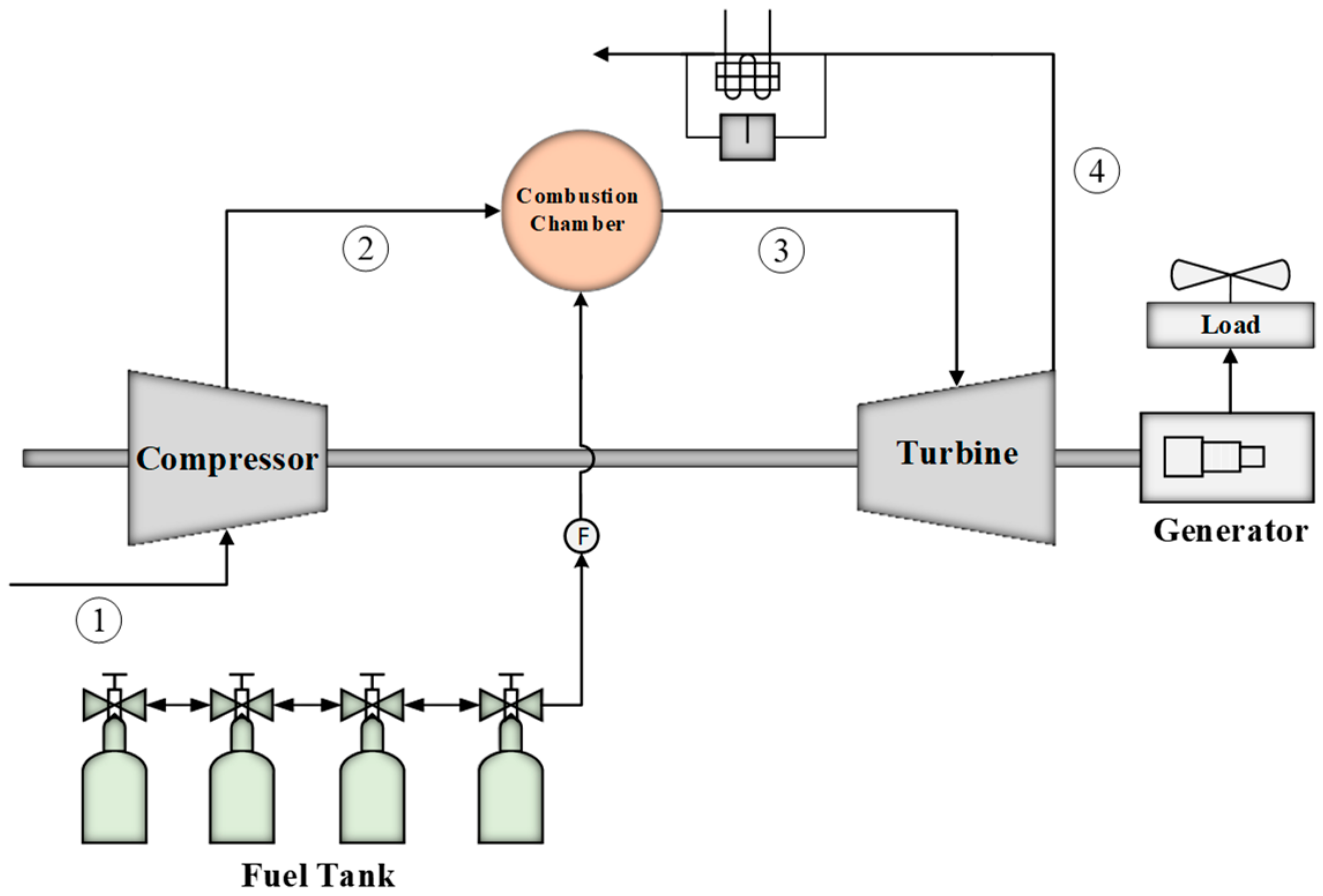
Figure 2.
Energy modeling algorithm for gas turbines.
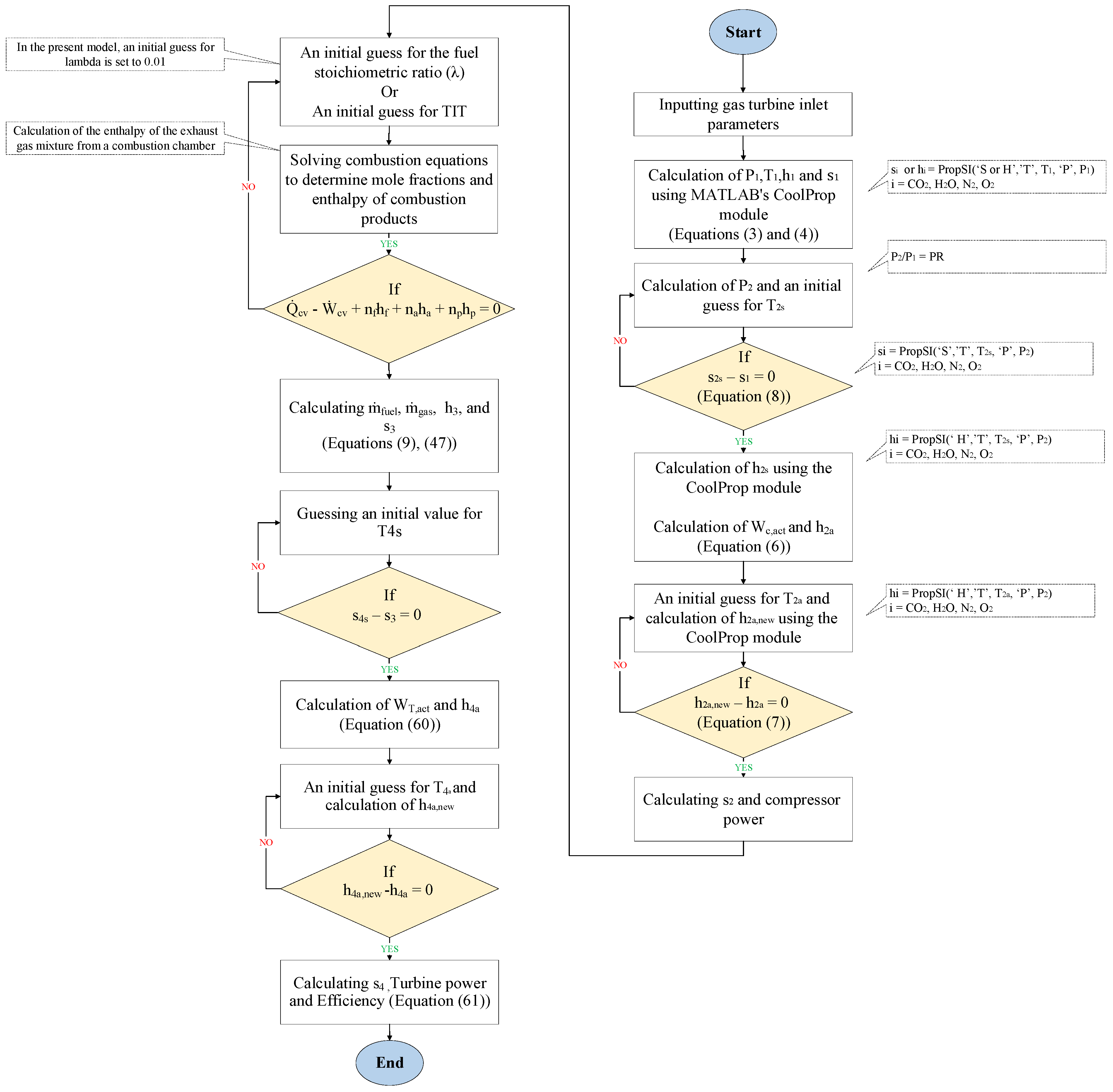
Figure 3.
Modified Genetic Algorithm.
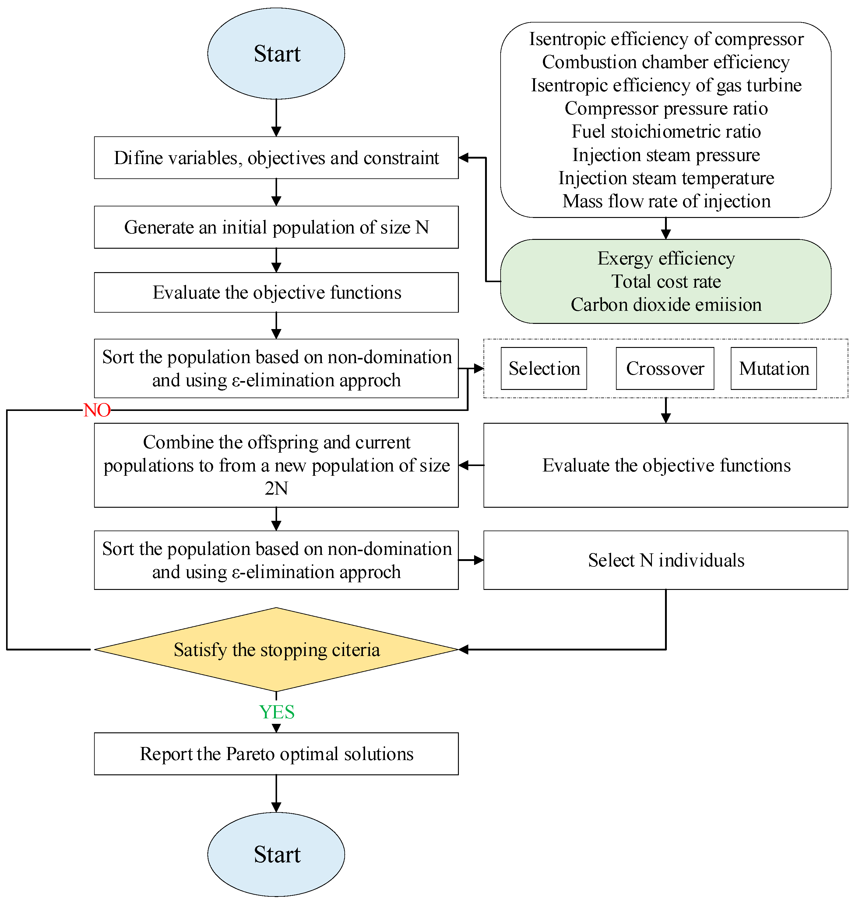
Figure 4.
Comparison of (b) exergy efficiency and (a) exergy destruction in different components of a gas turbine.
Figure 4.
Comparison of (b) exergy efficiency and (a) exergy destruction in different components of a gas turbine.
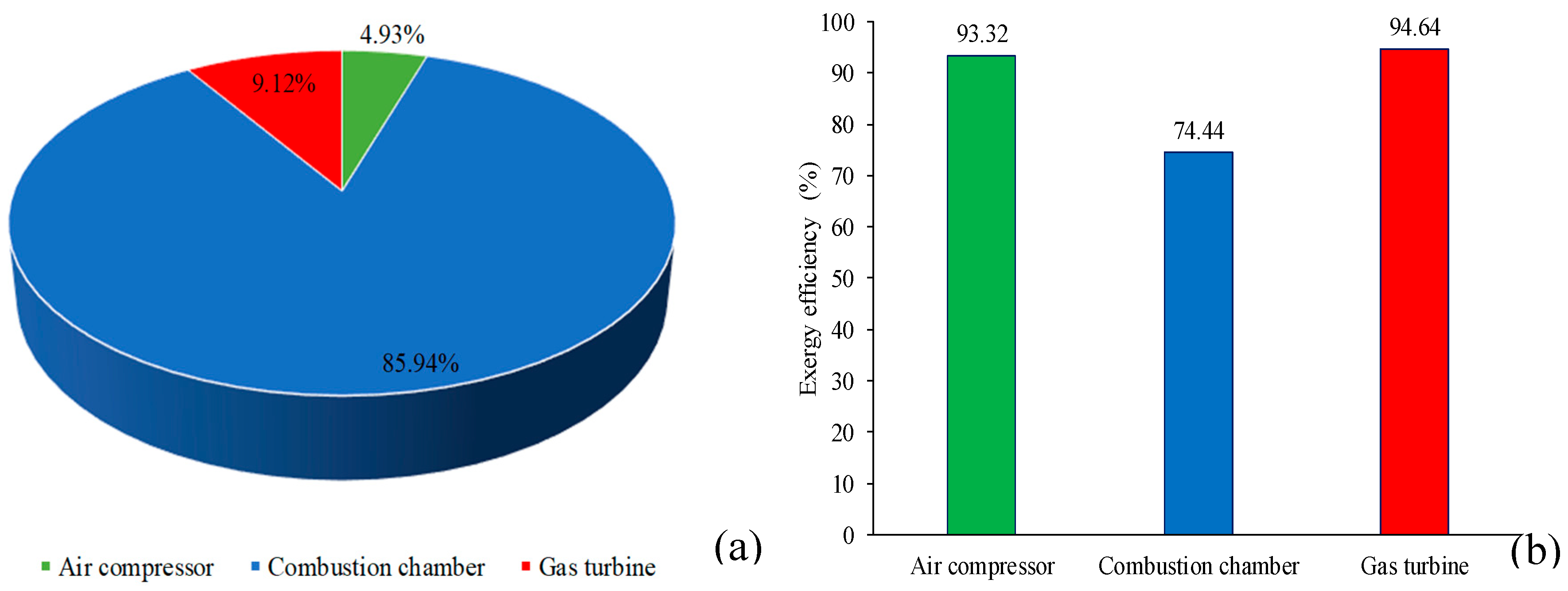
Figure 5.
Effect of and on Exergy Efficiency (Without Steam Injection).
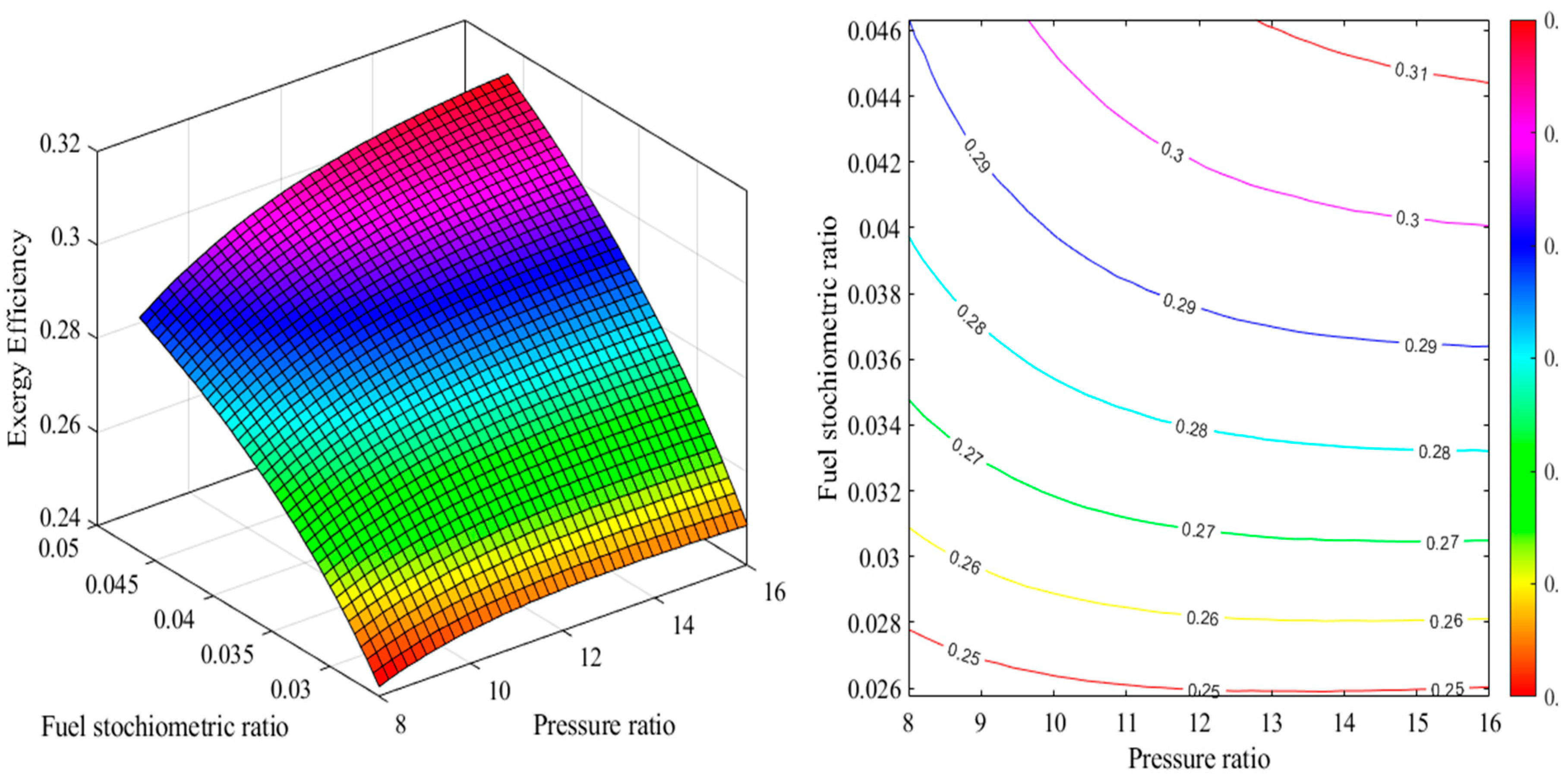
Figure 6.
Effect of and on Total Cost Rate (Without Steam Injection).
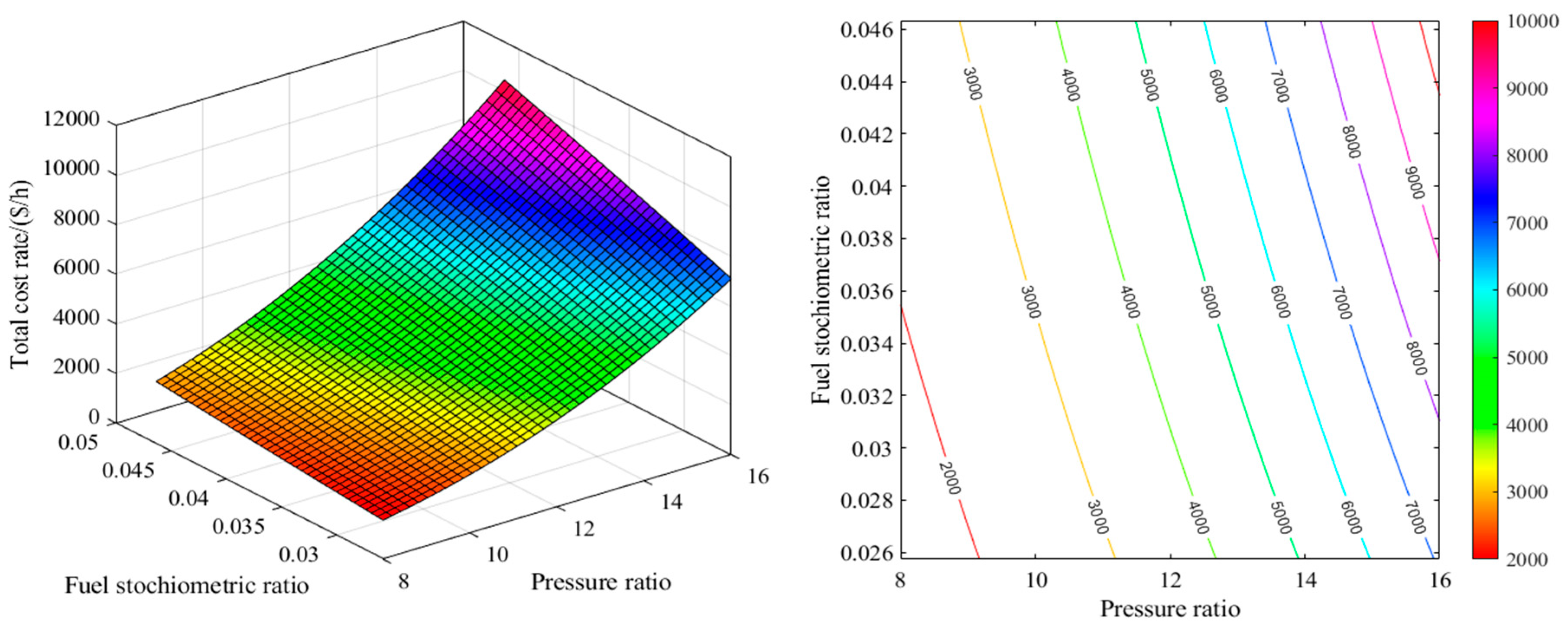
Figure 7.
Effect of and on CO2 index (Without Steam Injection).
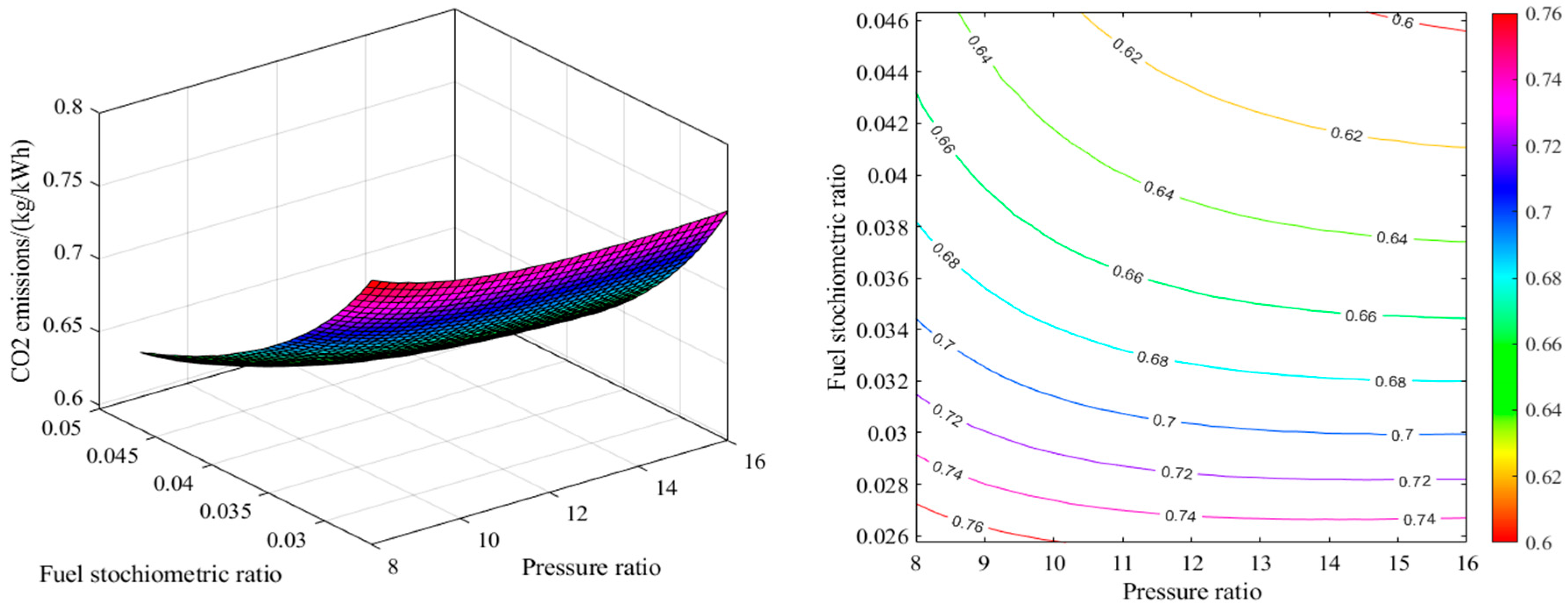
Figure 8.
Effect of and on Exergy Efficiency.
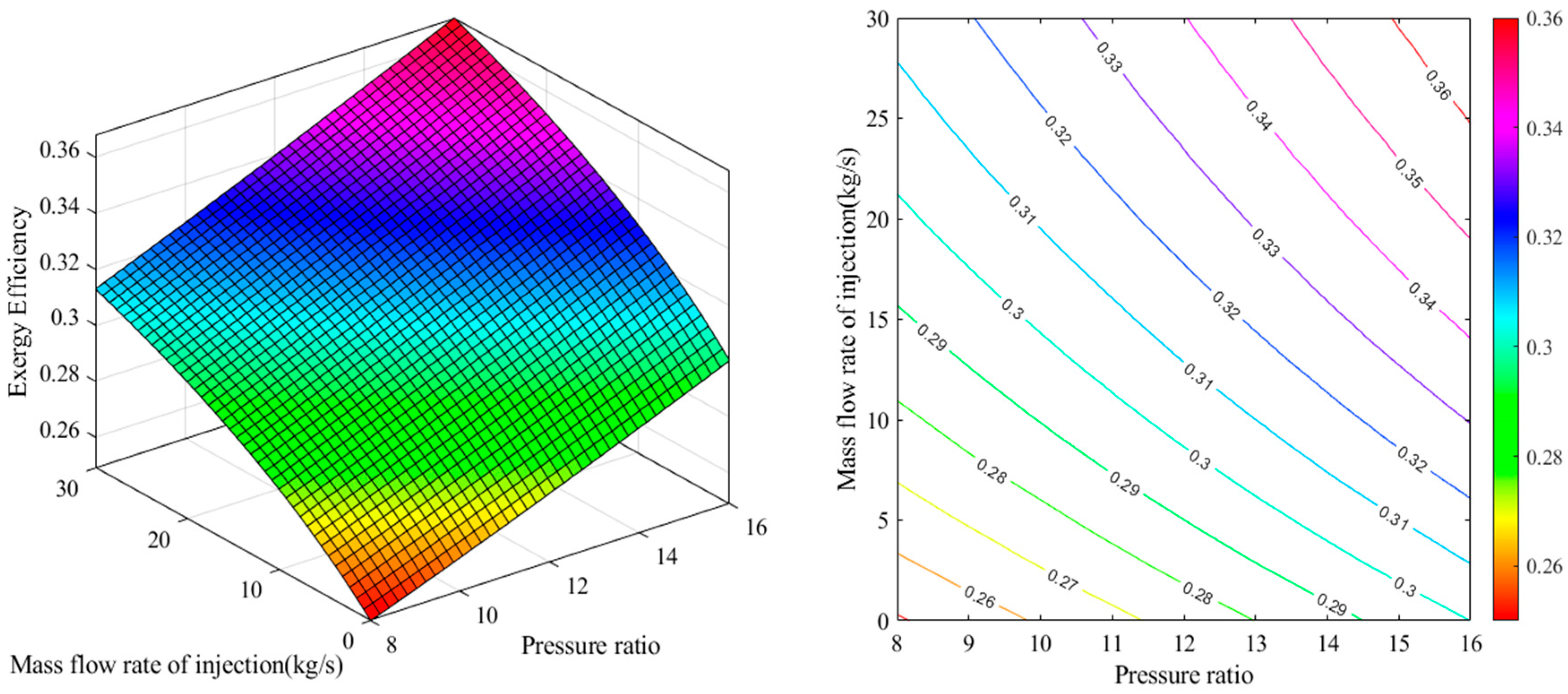
Figure 9.
Effect of and on Total Cost.
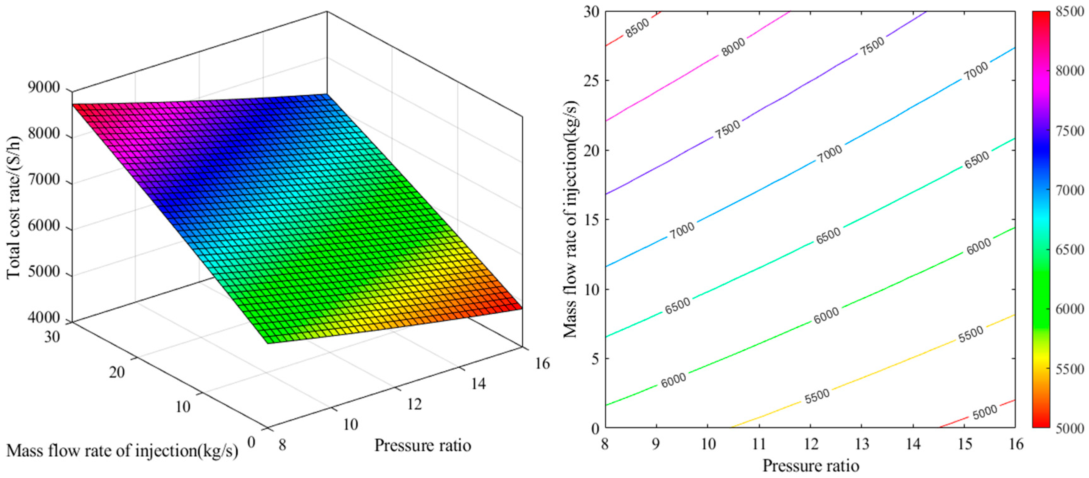
Figure 10.
Effect of and on CO2 Emission Rate.
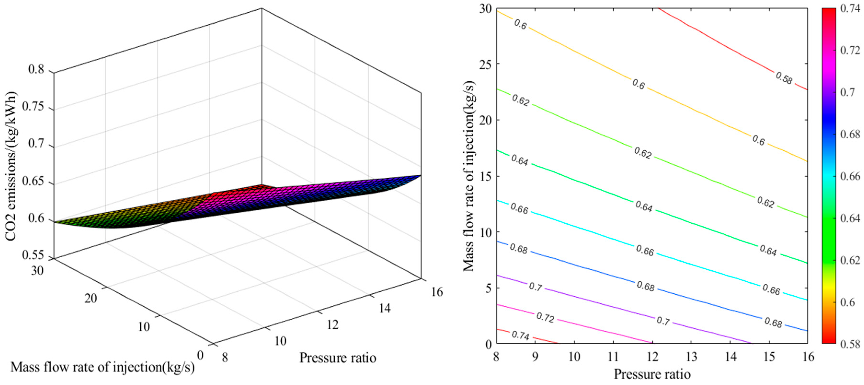
Figure 11.
Effect of and on Exergy Efficiency.
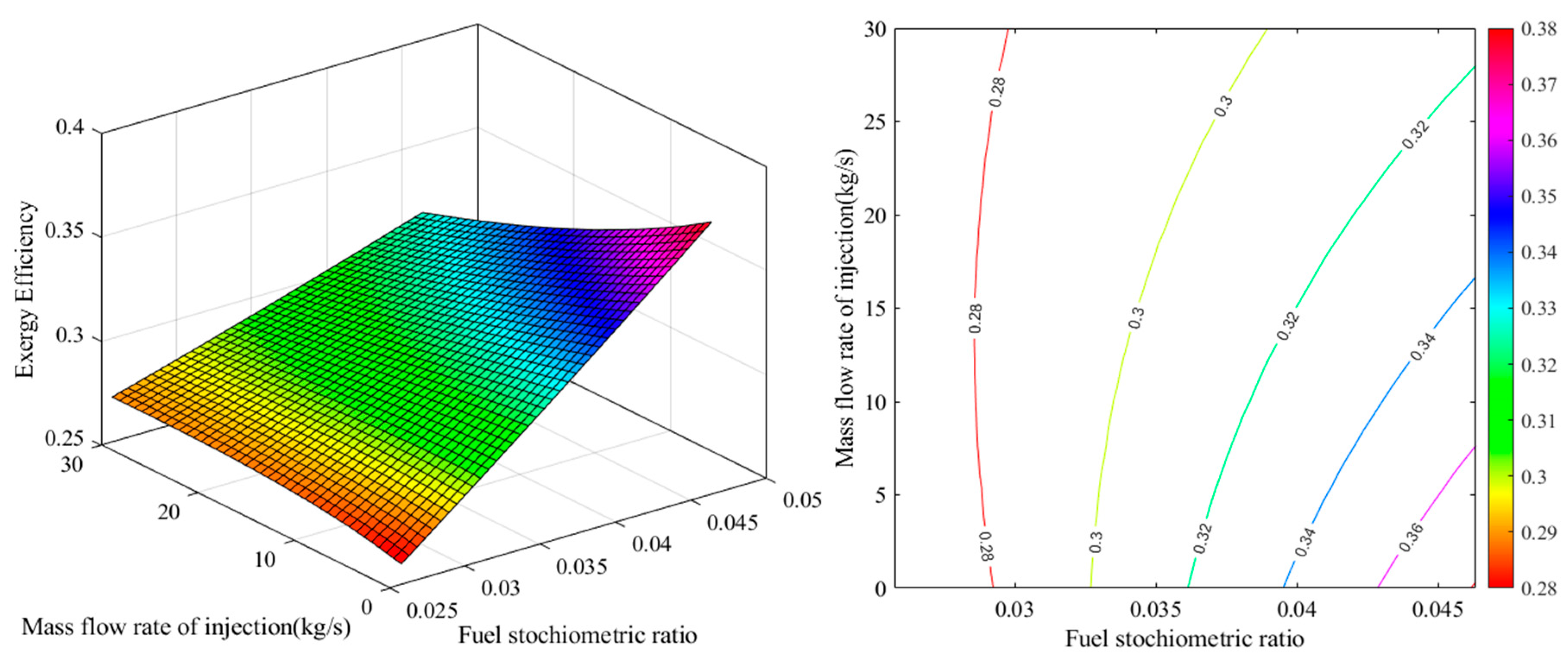
Figure 12.
Effect of and on Total Cost.
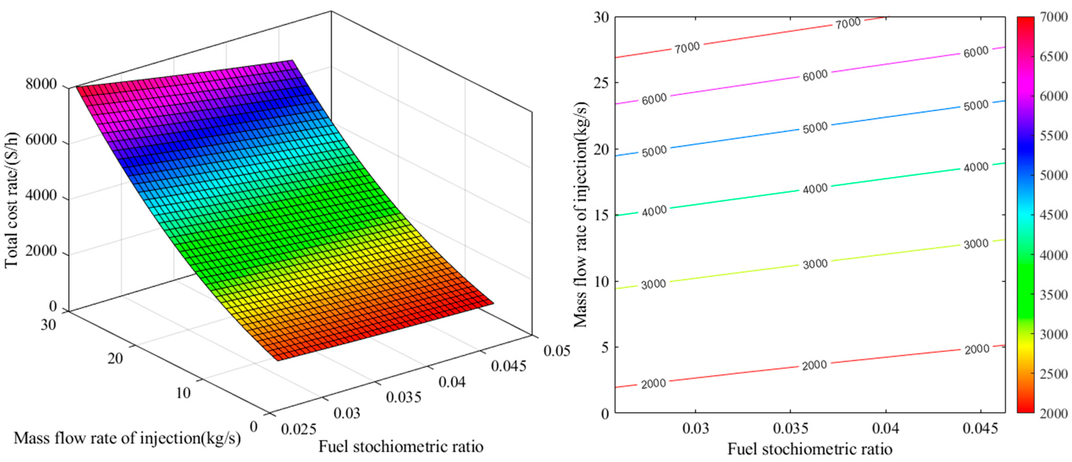
Figure 13.
Effect of and on CO2 Emission Rate.
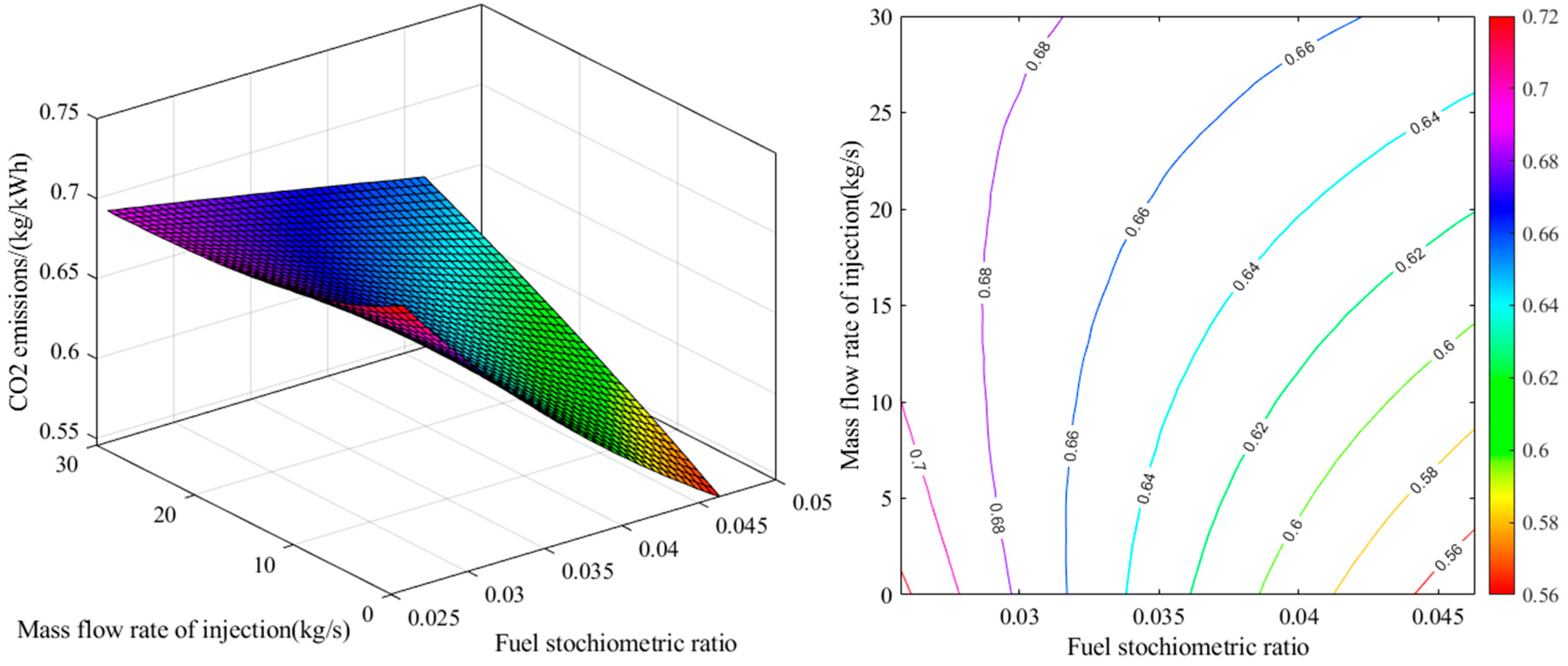
Figure 14.
The effects of parameter on NO and CO Emissions.
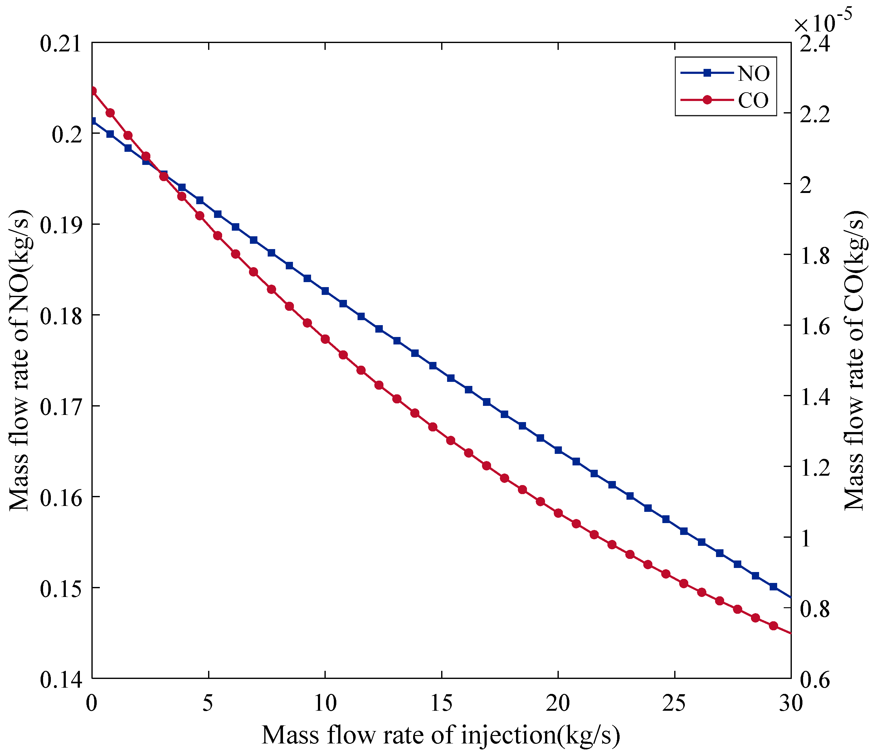
Figure 15.
The effects of parameter on TIT.
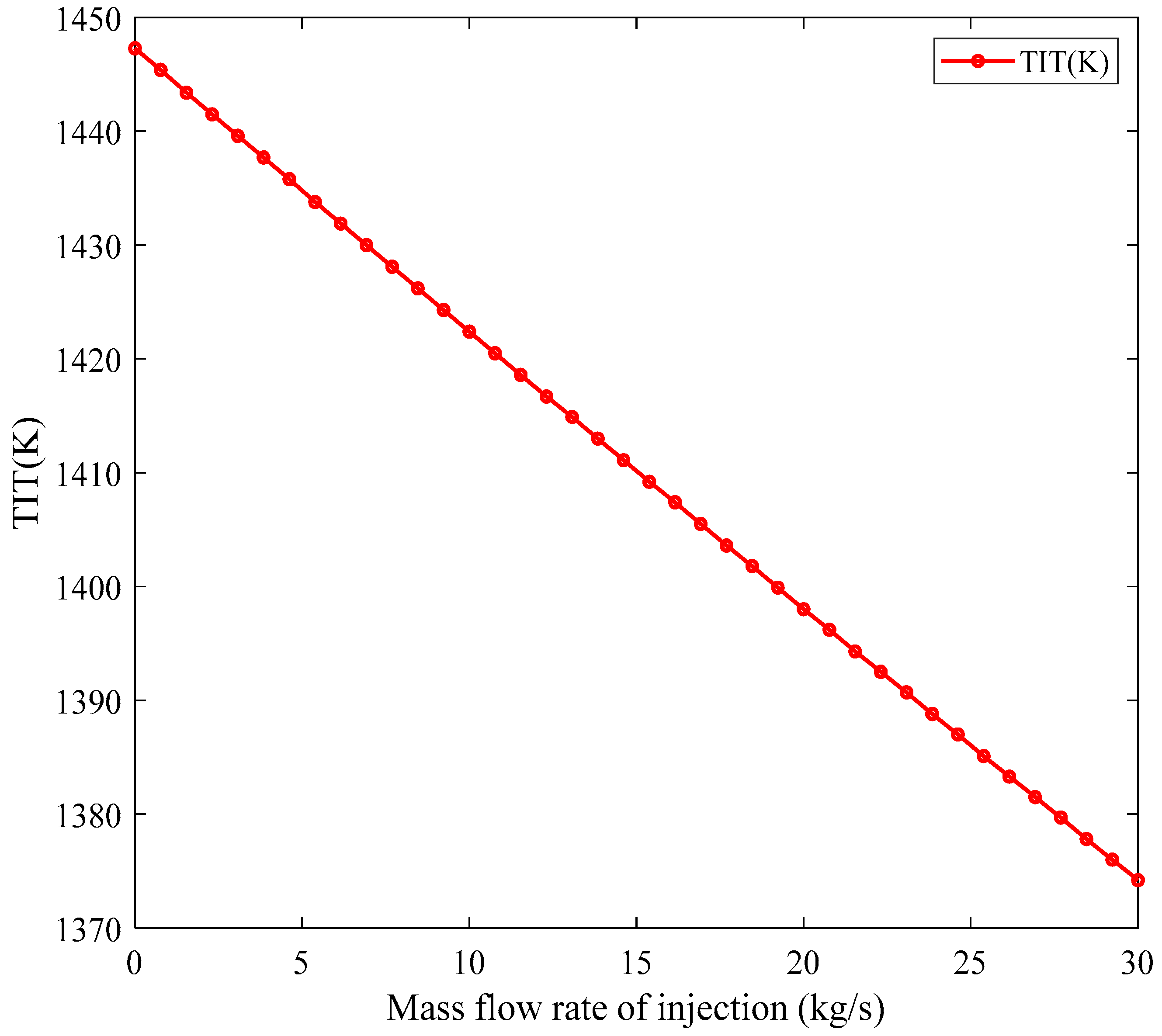
Figure 16.
Pareto front for multi-objective optimization of exergy efficiency, CO2 index and total cost rate.
Figure 16.
Pareto front for multi-objective optimization of exergy efficiency, CO2 index and total cost rate.
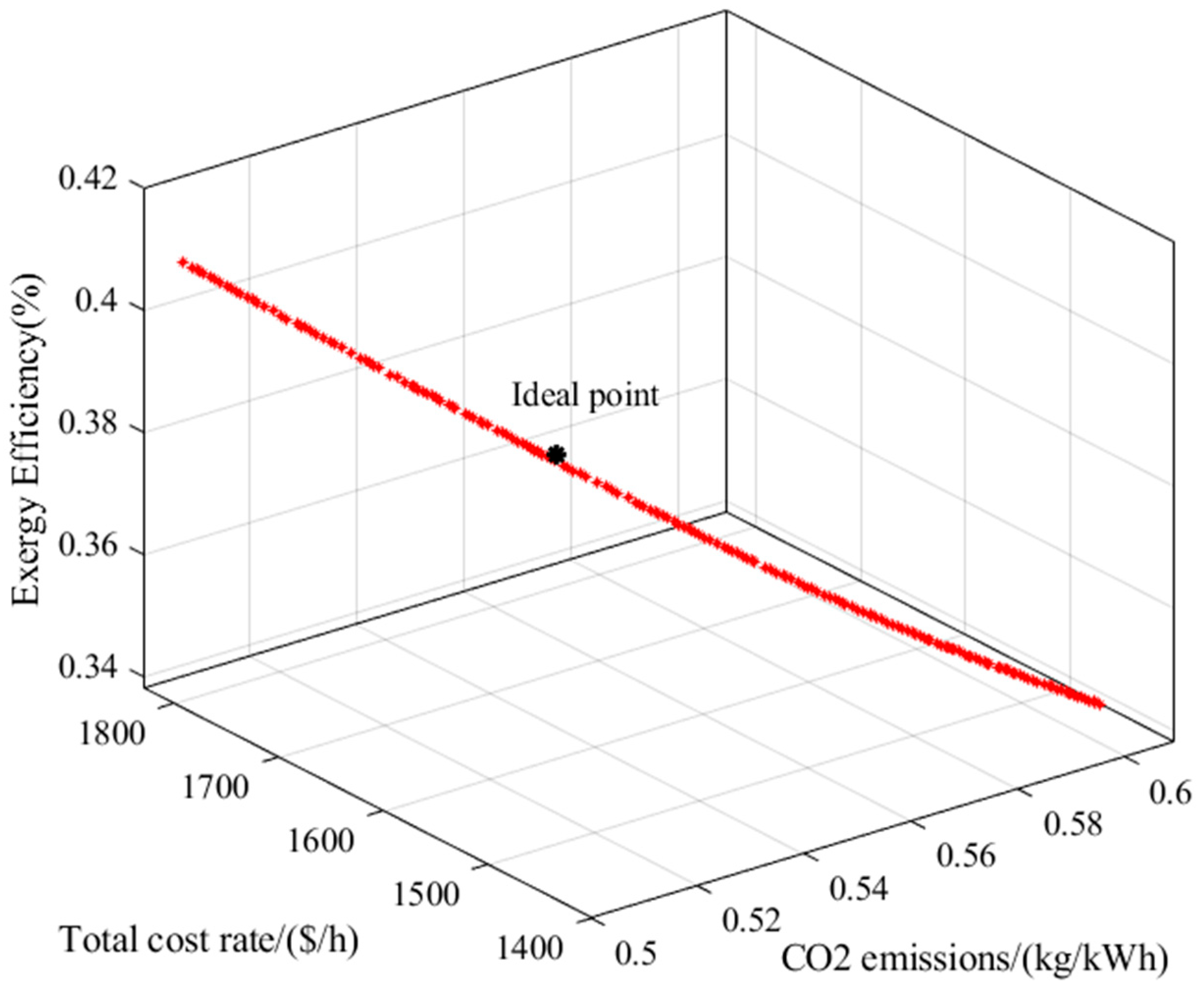
Figure 17.
Distribution of compressor and combustion chamber efficiencies.
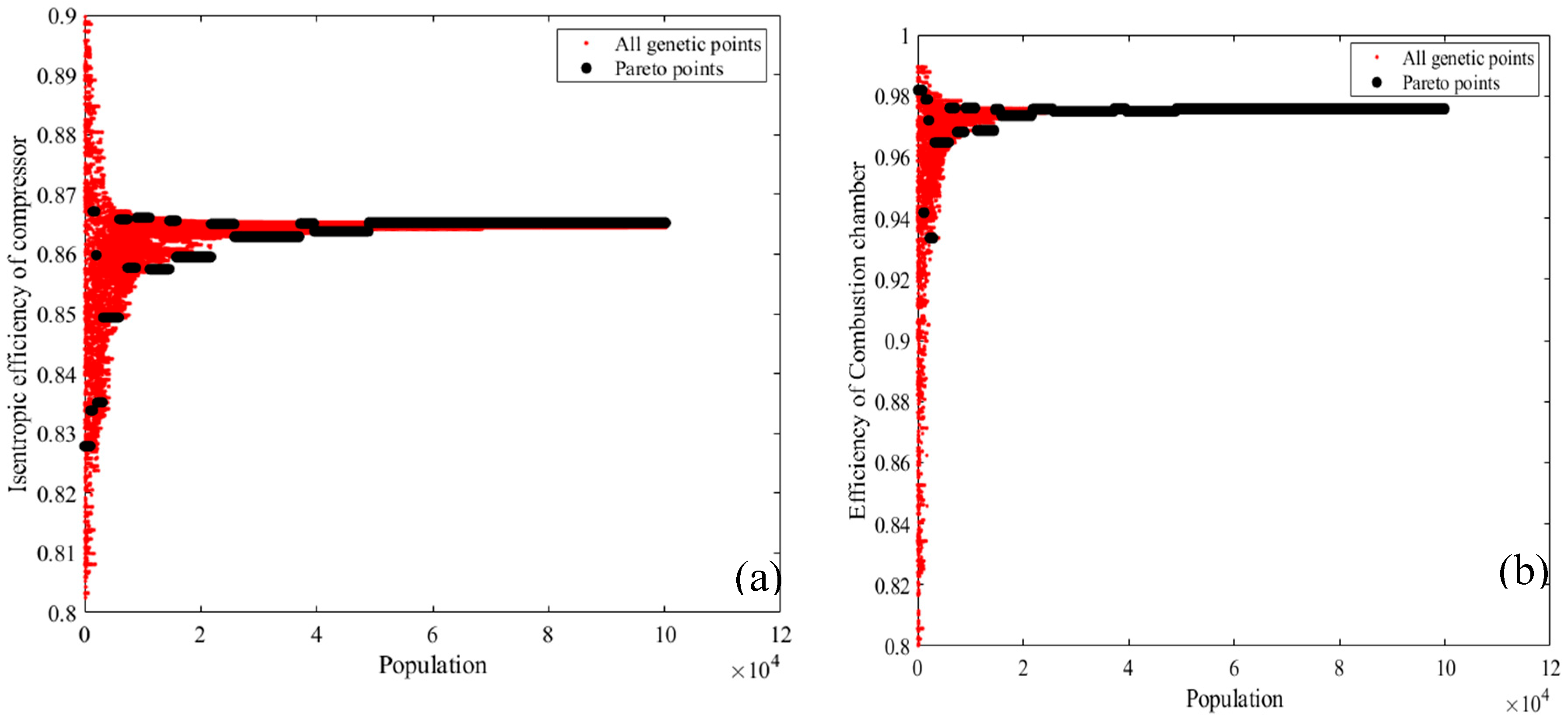
Figure 18.
Distribution of turbine efficiency and injected steam mass flow rate.
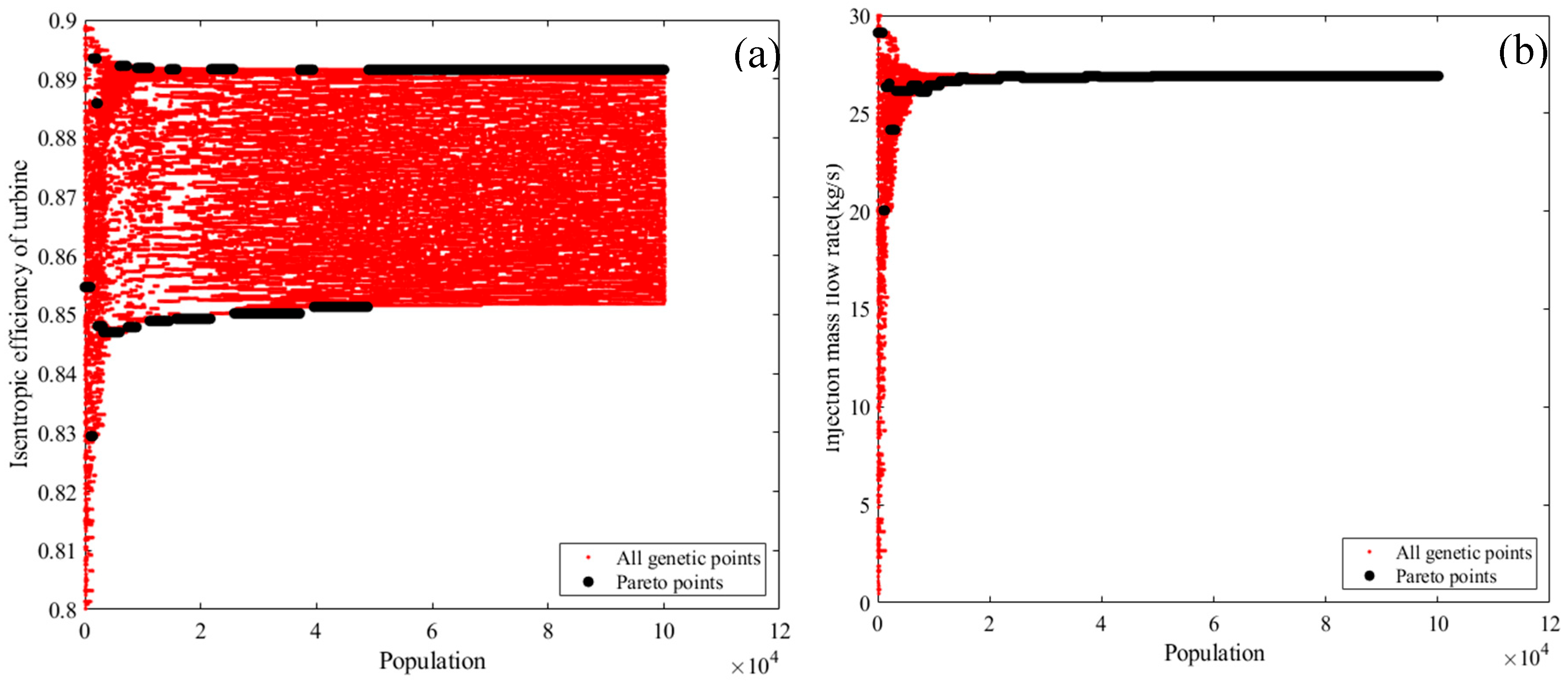
Figure 19.
Distribution of stoichiometric fuel ratio and compressor pressure ratio.
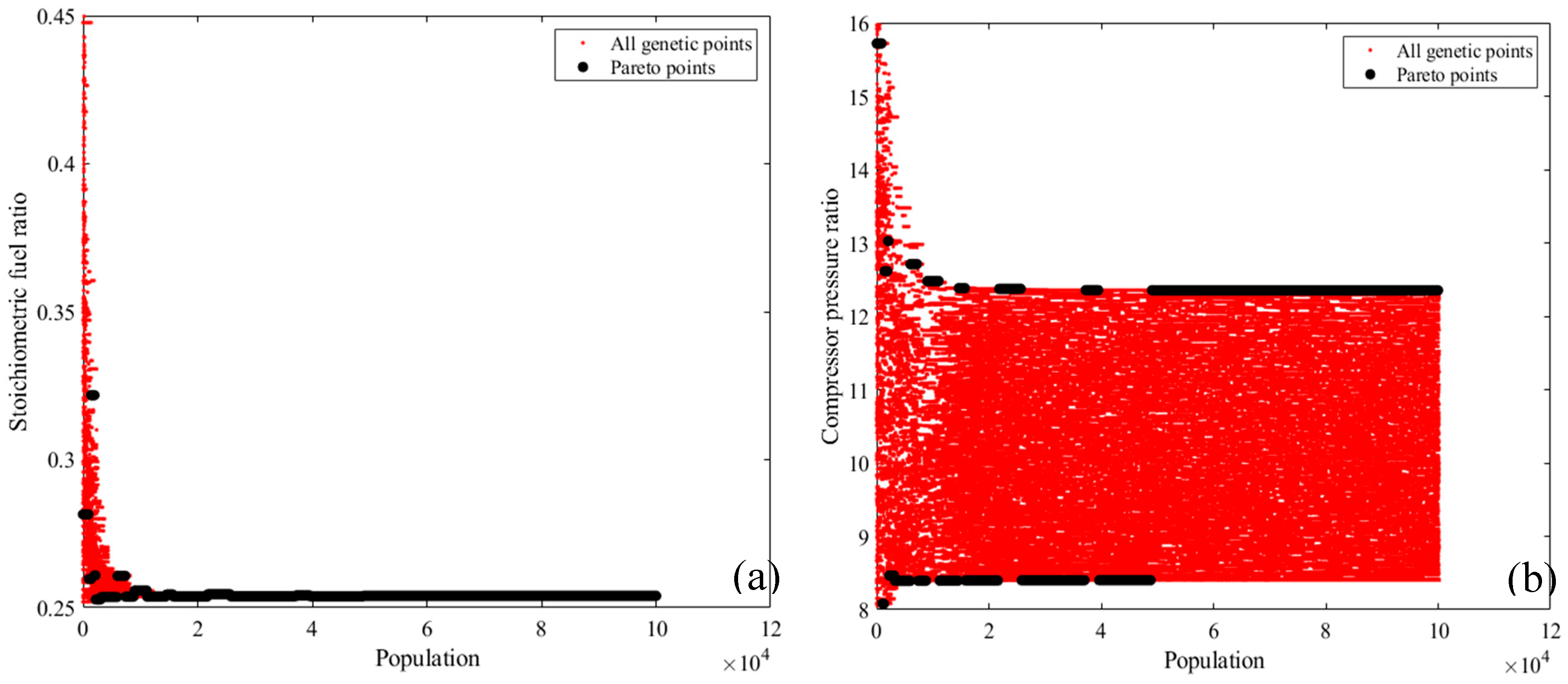

Table 1.
Coefficients of the equilibrium constants employed in equation (15) [21].
Table 1.
Coefficients of the equilibrium constants employed in equation (15) [21].
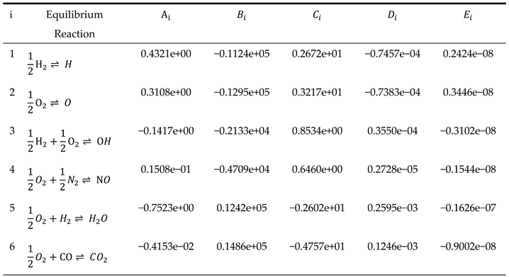 |
Table 2.
Combustion products for initial estimation of mole fractions.
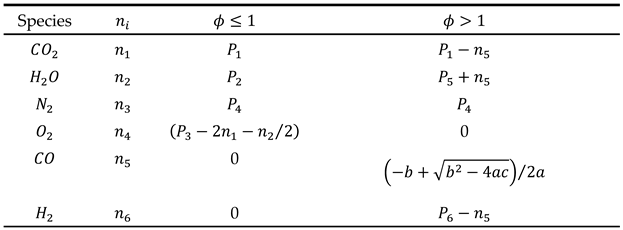 |
Table 3.
Equations used to calculate the exergy efficiency and exergy destruction in various components of a gas turbine [28,29].
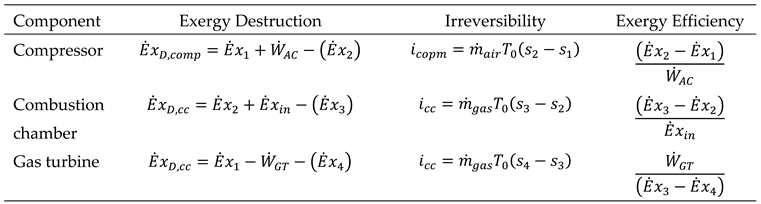 |
Table 4.
Auxiliary equations and cost balance equations for gas cycles [30].
Table 4.
Auxiliary equations and cost balance equations for gas cycles [30].
|
Table 5.
Formulation of equipment purchase cost for all components [30].
Table 5.
Formulation of equipment purchase cost for all components [30].
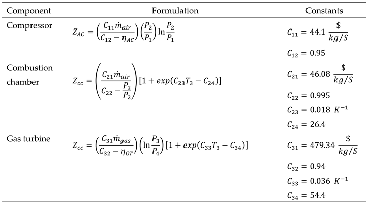 |
Table 6.
Comparison of the results of the present combustion model with those obtained from the commercial software GASEQ and CEA for methane fuel under .
Table 6.
Comparison of the results of the present combustion model with those obtained from the commercial software GASEQ and CEA for methane fuel under .
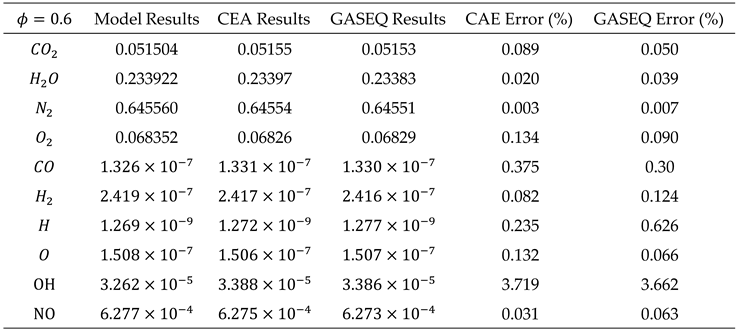 |
Table 7.
Comparison of the results of the present combustion model with those obtained from the commercial software GASEQ and CEA for methane fuel under .
Table 7.
Comparison of the results of the present combustion model with those obtained from the commercial software GASEQ and CEA for methane fuel under .
|
Table 8.
Validation of the proposed model against the reference data [32].
Table 8.
Validation of the proposed model against the reference data [32].
| Components | (MW) | |
| Present Study | Ameri et al [32]. | |
| Compressor | 6.02 | 5.99 |
| Combustion Chamber | 143.12 | 142.51 |
| Gas Turbine | 21.11 | 21.01 |
Table 9.
Input Parameters for the Gas Turbine (GE 9E model) [14].
Table 9.
Input Parameters for the Gas Turbine (GE 9E model) [14].
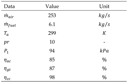 |
Table 10.
Decision Variable Ranges.
 |
Disclaimer/Publisher’s Note: The statements, opinions and data contained in all publications are solely those of the individual author(s) and contributor(s) and not of MDPI and/or the editor(s). MDPI and/or the editor(s) disclaim responsibility for any injury to people or property resulting from any ideas, methods, instructions or products referred to in the content. |
© 2025 by the authors. Licensee MDPI, Basel, Switzerland. This article is an open access article distributed under the terms and conditions of the Creative Commons Attribution (CC BY) license (http://creativecommons.org/licenses/by/4.0/).
Copyright: This open access article is published under a Creative Commons CC BY 4.0 license, which permit the free download, distribution, and reuse, provided that the author and preprint are cited in any reuse.


