
Submitted:
01 August 2025
Posted:
04 August 2025
You are already at the latest version
Abstract
We propose a variant of Bayesian optimisation in which probability distributions are constructed using uncertainty quantification (UQ) techniques. These distributions serve as prior knowledge of the search space. They are introduced into the acquisition function to provide an enhanced guide to selecting enrichment points. Different versions of the proposed method are analysed, depending on the type of distribution used (normal, lognormal, etc.), and compared with traditional Bayesian optimisation using test functions. The results demonstrate competitive performance with selective improvements depending on problem structure, achieving faster convergence in specific cases. As an application, we consider a structural shape optimisation problem. The initial geometry is that of an L-shaped plate, and the aim is to minimize the volume subject to a horizontal displacement constraint expressed as a penalty. In this case, our approach acts as an initial step to quickly identify a promising region, while efficiently training the underlying surrogate model in said regions. Next, a gradient-based optimisation process adjusts the final design, harnessing the trained surrogate, leading to a volume reduction of more than 30% while satisfying the displacement constraint and incurring no new functional evaluations of the true and expensive objective.
Keywords:
bayesian optimization
; hilbert expansions
; bayesian inference
; uncertainty quantification
1. Introduction
Optimization of expensive-to-evaluate black-box functions is a problem found in a wide range of technological and engineering applications [1,2,3]. Two broad application fields include the tuning of Machine Learning (ML) and general Artificial Intelligence (AI) models[4,5,6], as well as multiple forms of engineering design optimization, such as shape, topology, and material optimization, spanning from structural to electronic engineering [7,8,9]. In both fields, complex computational models are required to compute the objective or performance function, resulting in elevated computation time for each evaluation of the objective. Additionally, these models act as black boxes, meaning that general properties of the underlying model (such as its derivative or gradient) are not available.
Bayesian Optimization (BO) is an optimization framework particularly well-suited to address the aforementioned black-box, expensive-to-evaluate optimization problem [10,11,12,13,14]. It harnesses the efficacy of a surrogate model to approximate the objective function. It utilizes a Bayesian predictor (an Acquisition function) of promising enrichment points that are likely to improve the prediction of the surrogate in regions of interest, that is, regions where the optimum is likely to be found based on the limited information available.
Ideally, an instance of BO balances exploration and exploitation [15] by combining the prediction and uncertainty of the surrogate, usually a Gaussian Process (), with the acquisition function [16,17].
Since BO is Bayesian in nature, its performance depends on the quality of the prior structure used in the model. No single prior can be ideal to capture every type of objective function (NFL principle), and a misguided prior may lead to unfeasible requirements in terms of functional evaluations, or to failure to converge towards a feasible optimum. In this sense, several versions of BO have explored ways to incorporate adapted priors into the basic BO algorithm [18,19], to accelerate convergence. In particular, Bayesian optimization with a prior for the optimum (BOPrO) [20] and related methods introduce a belief based on expert knowledge, which allows certain regions of the input space to be favoured as more promising. Strictly speaking, these approaches codify a form of prior that stems from the user’s previous experience and guide the acquisition function to explore such regions.
This article presents an algorithm that combines the advantages of classical Bayesian optimisation with prior distributions constructed from an initial experimental design (DoE, Design of Experiment), based on Uncertainty Quantification (UQ) techniques. While both the metamodel and prior distributions utilize the same DoE, they encode complementary information about the problem. While the metamodel seeks to approximate the objective function across the entire domain, taking advantage of spatial correlations between samples, the prior distributions quantify the search space in a Bayesian sense by identifying regions where the objective is likely to attain good or bad performance contingent on the observations.
In engineering contexts, expert priors are often unavailable or difficult to justify, particularly in early design phases. In such cases, investing in a small exploratory DoE enables data-driven prior construction that can guide the optimization process efficiently from the outset, as demonstrated in this work.
The organization of this article is the following: Section 2 reviews the fundamentals of Bayesian optimization and the original BOPrO scheme. Section 3 details the construction of the UQ-based performance prior and its integration into the complete algorithm. Section 4 presents numerical results from six academic test functions and a case study from an engineering application, highlighting the applicability of the proposed method. Finally, Section 5 summarizes the conclusions and outlines future research directions.
2. Background
We are interested in solving the following global optimization problem:
where is the function to be minimized.
Sequential Bayesian estimation gives rise to a global optimization framework, commonly referred to as BO, which is particularly suited for problems such as the one described above. BO relies on the fundamental principle of Bayesian updating. A typical iteration of a Bayesian Optimization Algorithm (BOA) proceeds as follows [21]:
- Generate a surrogate model of the objective function f, usually under the form of a Stochastic Process,
- Select a new point to evaluate the true objective function,
- Update the surrogate model using the Bayesian Update, the pair of the new point and the value of the objective function in it.
2.1. SBO
The most commonly used surrogate model in BOA is the [14,15,16,17,22,23]. A generalizes the multivariate Gaussian distribution to an infinite-dimensional stochastic process, where any finite collection of function evaluations follows a joint multivariate normal distribution. Just as a standard Gaussian distribution describes a random variable by its mean and covariance, a defines a distribution over functions, fully specified by a mean function and a covariance (or kernel) function [15]:
where the mean function is often set to zero, , and the covariance matrix has elements , with k denoting a positive semi-definite kernel function. Equation (2) represents the prior distribution induced by the , encoding assumptions about the smoothness and structure of the underlying objective function.
In terms of Bayesian update, the choice of a greatly simplifies the procedure, as the is conjugate to itself. This property ensures that the posterior distribution remains a , and that the update merely involves a straightforward modification of the mean and covariance functions [21]. More precisely, we assume that a set of observations, , has already been collected from previous iterations, where the outputs are noise-free evaluations of a deterministic function, i.e., . Let, , denote the vector of corresponding observations. Then, Bayes’ theorem yields the posterior distribution [15]:
the posterior distribution , which remains a due to the aforementioned conjugacy. This updated distribution leads to the following expression for the predictive distribution at any next evaluation point , which follows a univariate Gaussian distribution [15]:
with the predictive mean and variance given by:
where, . To select the next point , in BOA one must solve an auxiliary optimization problem involving the maximization of the acquisition function . Among the popular acquisition functions, we can cite the Expected Improvement (EI). Let denote the best (i.e., lowest) function value observed up to iteration t, and assume the predictive distribution at follows Equations (4) and (5). Then, the EI at a candidate point is defined as follows [21]:
A second popular acquisition function is the Probability of Improvement (PI):
Notice that:
Another advantage of is that they allow the obtaining of closed analytical expressions for the EI and PI. Let and , respectively, be the cumulative distribution function and the probability density function of the standard normal distribution . Since the predictive distribution at a candidate point is Gaussian with mean and standard deviation , the EI can be calculated as follows [21]:
with,
Similarly, the PI can also be expressed as:
Throughout this article, we will refer to Standard Bayesian Optimization (SBO) as the Bayesian optimization framework where the surrogate model is a and the acquisition function is the EI.
To illustrate how the SBO works in practice, we will consider a one-dimensional synthetic test function proposed by Gramacy and Lee [24]. The objective is to find the global minimum of this function:
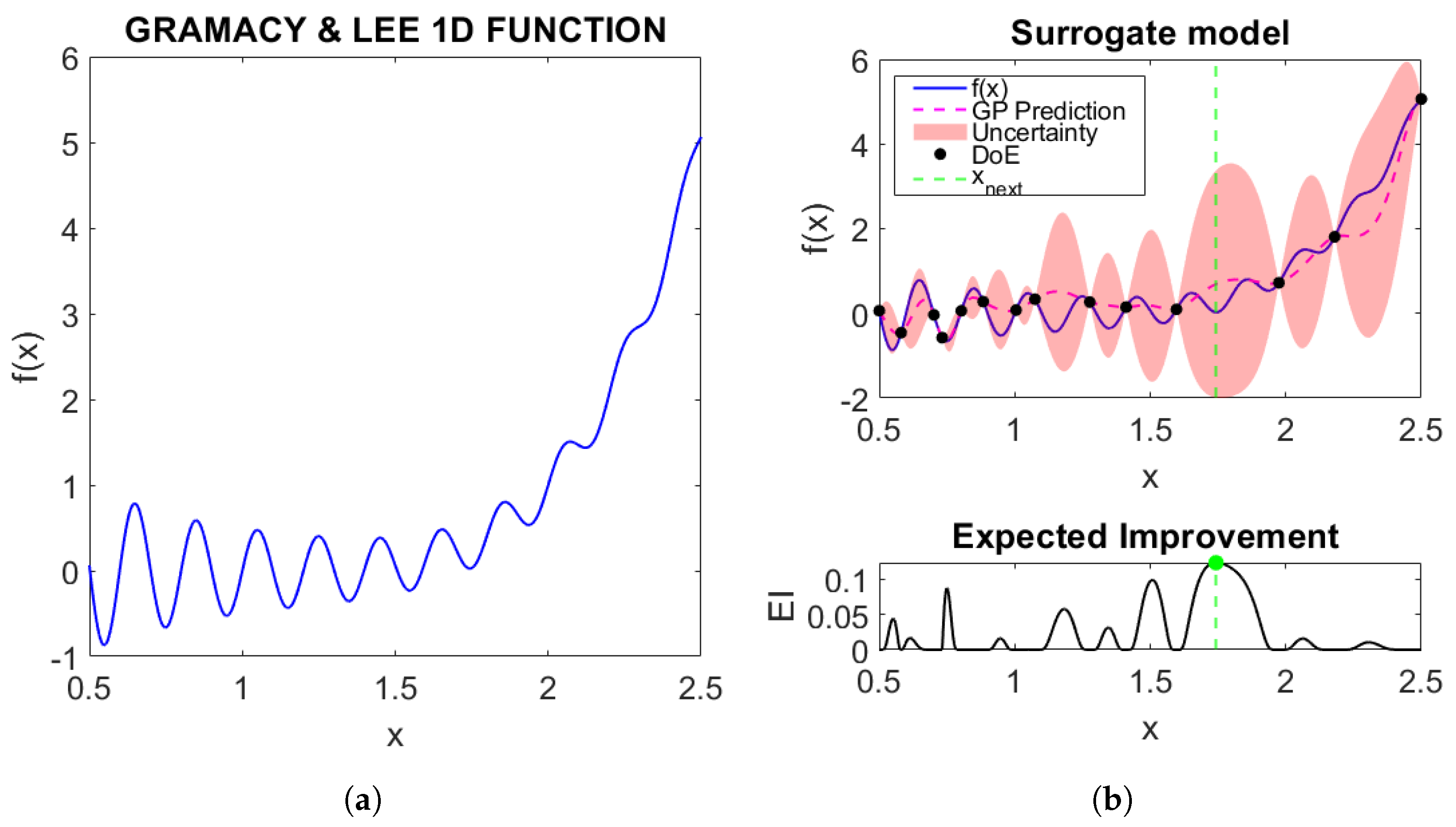
Figure 1.
Illustration of the SBO optimization process. Figure (a) shows the shape of the function we want to optimize, and Figure (b) shows the mean (prediction) of the surrogate model with the associated uncertainty, as well as the structure of the EI and its maximum.
Figure 1.
Illustration of the SBO optimization process. Figure (a) shows the shape of the function we want to optimize, and Figure (b) shows the mean (prediction) of the surrogate model with the associated uncertainty, as well as the structure of the EI and its maximum.
2.2. BOPrO
Bayesian optimization with a prior for the optimum (BOPrO), proposed by Souza et al. [20], is a recently developed version of BO based on the tree-structured Parzen estimator (TPE) [25], which allows users to introduce intuitive domain knowledge into the optimization process. These priors do not modify the surrogate model (e.g., a ). However, they are combined with the probability of improvement (PI) to form what is called a pseudo-posterior, more precisely, a posterior pseudo-density because it is not necessarily normalized (does not necessarily integrate to 1 in the prescribed domain), and acts as a weighting function inspired by Bayesian updating. This function is used in the acquisition function, in particular in the calculation of the modified expected improvement, which implies that the prior directly rebalances the weights assigned to the different regions of the search space in the EI evaluation. Thus, regions favoured by the prior are more likely to be explored at the beginning of the iteration process. As the iterations progress, the weight of the prior decreases, and the influence of the predictive model dominates the search.
The mathematical expression corresponding to this modified version of the expected improvement criterion, adopted by BOPrO to effectively integrate the pseudo-posterior into the process of selecting new points, is formally derived from the TPE framework. It reads:
where g and b are non-normalized density functions describing, respectively, the promising and less promising areas of the search space. The value acts as a quantile threshold that determines at what point a function value can be considered “good”.
The main contribution of BOPrO is the practical implementation of this performance pseudo-posterior. In the case of , a prior distribution is integrated, reflecting the user’s belief about promising regions, together with a probability derived from the model , which represents the possibility, under the surrogate -that the value of the function falls below a threshold . Which we can express as follows:
The density for the unpromising regions is given by:
where , represents the prior for bad regions, t is the current iteration and hyperparameter defines the balance between prior and model, with higher values giving more importance to the prior and requiring more data to overrule it [20].
The probability is defined as follows:
and the probability for unpromising regions is given by:
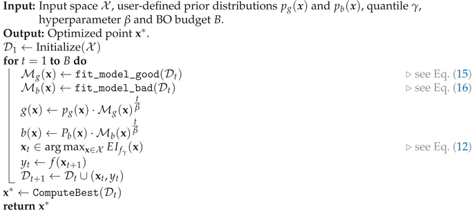
Algorithm 1 describes in detail the optimization process carried out by BOPrO.
| Algorithm 1: BOPrO Algorithm. keeps track of all function evaluations so far: [20]. |
 |
3. Data-Driven Prior Construction in Hilbert Spaces for Bayesian Optimization
3.1. Preliminaries
The BOPrO framework is a technical development adapted for machine learning applications, with the properties of the algorithm crafted explicitly for this type of problem. The performance priors are established in a way that facilitates use by an ML expert with domain knowledge in hyperparameter tuning. The goal is to provide a practical tool to codify this expert knowledge into a prior that: 1) describes the belief that certain regions of the search space are more (respectively, less) promising; 2) can be combined with the information available, both from model evaluations and from surrogate model predictions. This formulation poses significant limitations when the domain of application is different, such as structural design or general engineering design optimization. Notably, in such applications, expert knowledge may not be available, or sufficiently reliable, or the expert knowledge may be applied at a different stage of the process.
Our proposed method takes some of the central ideas in BOPrO (and the TPE algorithm). In particular, we retain the adapted version of the EI acquisition function and the structure of the priors over the search space, informing the early stages of the optimization iteration process. However, unlike the previous work, we replace the expert knowledge codified in the performance priors by systematic and reproducible distributions, learned directly from initial observations. To achieve this, we adopt the approach proposed by Souza and Fabro [26], which provides distributions that can be considered priors in a Bayesian procedure, particularly effective when data is limited.
3.2. Construction of Priors
The Hilbert Approach (HA), which can be viewed as an extension of Polynomial Chaos Approximations (PCA), can be applied under two basic conditions: is assumed to satisfy some basic conditions:
- The uncertainties can be modeled by a random vector U and the variable of interest is ;
- the random variable U takes its values on an interval of real numbers (or, more generally, on a bounded subset of );
- X belongs to the space of square summable random variables: , id est, X has finite moment of order 2;
- some statistical information about the couple is available.
These assumptions ensure that X can be represented by an infinite expansion involving a convenient orthonormal Hilbert basis , allowing one to represent X as [26,27]:
As previously observed, U is a suitable random variable used to construct a stochastic representation of X. Nevertheless, in practical situations, U can be an artificial variable, conveniently chosen [21,28]. Artificial variables are used, namely, when not any information is available about the source of randomness: then, U is chosen by the user and it is mandatory to create an artificial correlation between samples of the artificial variable and samples of X. For instance,we can range both in an increasing order: , and - this generates a non-negative covariance between X and the artificial U.
In practice, the expansion is truncated at order k, yielding an approximation :
The finite representation is determined by finding the coefficients . A popular method for the determination of is collocation, which considers a sample and solves the linear system [28]:
The reader can find in the literature works using such an approach. In general, (the system is overdetermined) and Equation (19) must be solved by a least squares approach. Once is determined, the representation can be used to generate the distribution of X. For instance, we can generate a large sample of variates from U (eventually, a deterministic one),
and use it to generate a large sample from X as , . Then, is used to estimate the cumulative distribution function (CDF) and probability density function (PDF) of X, by using the empirical CDF of the large sample.
From the Bayesian standpoint, estimates can be obtained by minimizing a loss function defined over the estimated PDF. This approach can be used to define a univariate parametric prior distribution , where the parametric family (e.g., Gaussian, log-normal) is selected by the user.
In the case of a multidimensional input, we assume independence between dimensions, so that the a priori multivariate distribution is constructed as the product of the univariate margins:
This independence hypothesis, although simplistic and not necessarily valid in all cases, is adopted here as a reasonable working assumption to facilitate model construction and advance the validation of the proposed ideas.
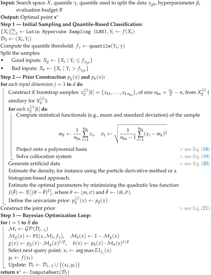
The full optimization procedure is detailed in Algorithm (2).
Let’s return to the practical case defined in Section 2, this time applying our proposed method. The objective is to visualise the interaction between the different elements of the proposed method: the surrogate model, the acquisition function, the prior distributions, and the update points. Using the same DoE, we analyse how the behaviour of the acquisition function differs between our approach and SBO. The prior distributions we propose allow us to identify regions of the search space that, although considered promising by the metamodel, receive a low probability (see Figure 2(b)). As a result, the algorithm avoids exploring these regions and selects a new point different from the one that the traditional approach would have chosen (see Figure 2(f)).
| Algorithm 2: Data-Driven Prior Construction in Hilbert Spaces for Bayesian Optimization |
 |
4. Results
In this section, we test our proposed method on six test functions and one engineering application. Our results are contrasted with SBO as a baseline. The test functions have been chosen to explore the general behavior of the method, even though they do not constitute expensive black-box functions. The application is a good representative of the kind of problem where BO is expected to excel.
Our focus here is exploratory, as we seek to identify interesting behavior of the proposed method against SBO, and with varied objective functions. We have thus selected performance metrics that reflect a mix of robustness(success rate), reliability (proximity to the optimum), and convergence speed (simple regret plots); moreover, particular attention is given to the variability of the method given different instances of the DoE, leading us to report extremes, averages and variances of each instance of our method for several runs.
4.1. Test Design and Technical Aspects
Our approach is evaluated by identifying the global minima of a set of test functions from the Virtual Library of Simulation Experiments [24].
Table A1 in Appendix A shows the mathematical expression, the problem size, the search space, the known global minimum, and the threshold considered as the success criterion. This threshold is defined by applying a relative error criterion of , using the following formula:
In the particular case of the Sum of Different Powers function, whose global minimum is zero, a target equal to is arbitrarily set to avoid zero values.
Different families of parametric distributions (e.g., Gaussian, log-normal, etc.) are fitted to the parameters estimated using the Hilbert approximation implemented in the proposed method and compared with SBO. Ten runs of the code are performed, each with a randomly generated DoE. An optimization budget equal to 15 × dimension is set. The size of the DoE is set to 10 × problem dimension. The hyperparameter was assigned values between 10 and 100. Two different values are used for the parameter :
- The first, , implemented within the optimization algorithm, takes values between 0.01 and 0.05.
- The second, , is used to divide the DoE into two subsets (good and bad) for the construction of the apriori.
4.2. Benchmark Problems
In addition to the box plot presented in Figure 3(a)-3(f), we provide complementary numerical results in Tables 1-6. For each test function and each prior distribution used in the HSBO framework, we indicate:
- the maximum and minimum values reached by the function (corresponding to the 10 runs) obtained in the last iteration. This allows us to capture the worst and best performance of the algorithm.
- the mean of the function values at the last iteration (corresponding to the 10 runs) and the standard deviation of these values.
- the success rate, defined as the number of executions in which the function reached a value below the target.
These statistics provide additional information about the stability and robustness of our proposal and allow us to evaluate how often a method successfully identifies a near-optimal solution.
To evaluate the performance of the algorithm across all iterations in the ten runs, the simple regret metric was used. Following the definition in [29,30], simple regret at iteration t is expressed as:
where is the global optimum of the objective function and denotes the set of points evaluated up to iteration t.
The mean simple regret obtained in the 10 runs is presented on a logarithmic scale in Figure A1 in Appendix B, which provides a clear comparison of the convergence speed of each configuration throughout the entire sequence of iterations.
4.2.1. Test Function a: Gramacy & Lee Function
Figure 3(a) shows the results obtained with the Gramacy & Lee function. It can be seen that both SBO and the proposed method with the Pearson distribution perform well. However, the mean of simple regret graph presented in Appendix B indicates that the Pearson distribution leads to faster convergence.
Table 1 shows that all methods manage to reach the theoretical minimum at least once. In terms of success rate, both SBO and the proposed method with Pearson distribution manage to find values below the target in all runs.

Table 1.
Performance at Final Iteration () over 10 Runs: Gramacy & Lee 1D Function
| Method | Min () | Max () | Mean () | Std() | Success rate ( target) |
|---|---|---|---|---|---|
| SBO (baseline) | -0.8690 | -0.8492 | -0.8648 | 10/10 | |
| HSBO with normal prior | -0.8690 | -0.6622 | -0.8407 | 9/10 | |
| HSBO with log-normal prior | -0.8690 | -0.6619 | -0.8271 | 8/10 | |
| HSBO with exponential prior | -0.8690 | -0.5185 | -0.8099 | 8/10 | |
| HSBO with Rayleigh prior | -0.8690 | -0.5185 | -0.7922 | 7/10 | |
| HSBO with Pearson prior | -0.8690 | -0.8492 | -0.8648 | 10/10 |
4.2.2. Test Function b: Cross-in-Tray 2D Function
Figure 3(b) shows the results obtained with the Cross-in-Tray function. It can be seen that both the normal and log-normal a priori distributions offer better performance compared to the SBO reference. Although SBO shares a low median, it has an outlier, indicating that in at least one run it deviated significantly from the optimum.
Table 2 confirms the observations made in the box plot: the normal and log-normal distributions achieve a success rate of 100% (10/10) and have a standard deviation lower than that of the baseline, indicating less variability between runs.
4.2.3. Test Function c: 2D Branin Function
Figure 3(c) shows the results obtained with the Branin function, where it can be seen that although the a priori-based configurations show competitive performance, in this particular case they fail to exceed the baseline (SBO).
Table 3 summarises the results obtained for the Branin function. It can be seen that the SBO method achieves the best average performance, with the lowest standard deviation and the highest success rate (6/10). In comparison, the HSBO configurations show greater variability and a reduced success rate, indicating that, in this case, the a priori assumptions do not provide a significant improvement over the baseline.
4.2.4. Test Function d: Hartmann 3D Function
Figure 3(d) shows the results for the Hartmann 3D function. It can be observed that both the baseline and the HSBO configurations with different prior distributions perform very similarly. The medians and dispersion of the relative errors are practically equivalent, suggesting that, in this case, none of the approaches offers a significant advantage over the others. This conclusion is reinforced by the numerical results presented in Table 4.
4.2.5. Test Function e: Sum of Different Powers (4D) Function
Figure 3(e) and Table 5 present the objective function values obtained at the end of the optimisation for the Sum of Different Powers function in dimension 4. Given that the global minimum is equal to zero, the most effective methods are those that achieve values closest to this threshold. In this regard, both SBO and HSBO with normal and Pearson distributions achieve outstanding performance, with very low final values and a 100% success rate. In contrast, configurations with lognormal, exponential and Rayleigh distributions have significantly higher function values and greater variability, indicating lower effectiveness for this problem.
4.2.6. Test Function f: Hartmann 6D Function
Finally, Figure 3(f) and Table 6 show the results obtained with the Hartmann 6D function. Although both SBO and the HSBO variants with different prior distributions achieve similar values close to each other, none of them comes close enough to the global minimum to meet the success criterion, which is reflected in a zero success rate for all cases. This result could indicate that, in problems of greater complexity or dimensionality, the number of iterations considered is not sufficient to allow effective exploration of the search space and reach the global optimum. Nevertheless, we highlight an interesting qualitative phenomenon in this particular case: the HSBO with lognormal prior continues to improve even after SBO has settled at a constant value. On average, SBO reaches a stable optimum around iteration 20. In contrast, HSBO-lognormal continues to improve around iteration 60, reaching a lower final average simple regret than SBO. This suggests an enhanced capability for exploitation for HSBO for this specific parametric prior.
4.3. Application: Shape Optimization of a Solid in Linear Elasticity Under Uniaxial Loading
A structural optimization problem is addressed in which the initial geometry, which is L-shaped, is parameterized using isogeometric analysis (IGA) on a finite element mesh constructed from NURBS surfaces [31]. The mechanical solver used is based on a MATLAB implementation of IGA in 2D linear elasticity, originally developed by Vinh Phu Nguyen (Johns Hopkins University) for educational and academic purposes1. This implementation includes the construction of stiffness matrices from NURBS, adaptive h refinement, and the treatment of natural and essential boundary conditions.
This code has been adapted to incorporate a shape optimization problem, in which the geometry of the L-shaped plate is perturbed by three design parameters that vertically modify certain NURBS control points. The design vector is denoted:
where each variable represents a vertical disturbance applied to a NURBS control point.
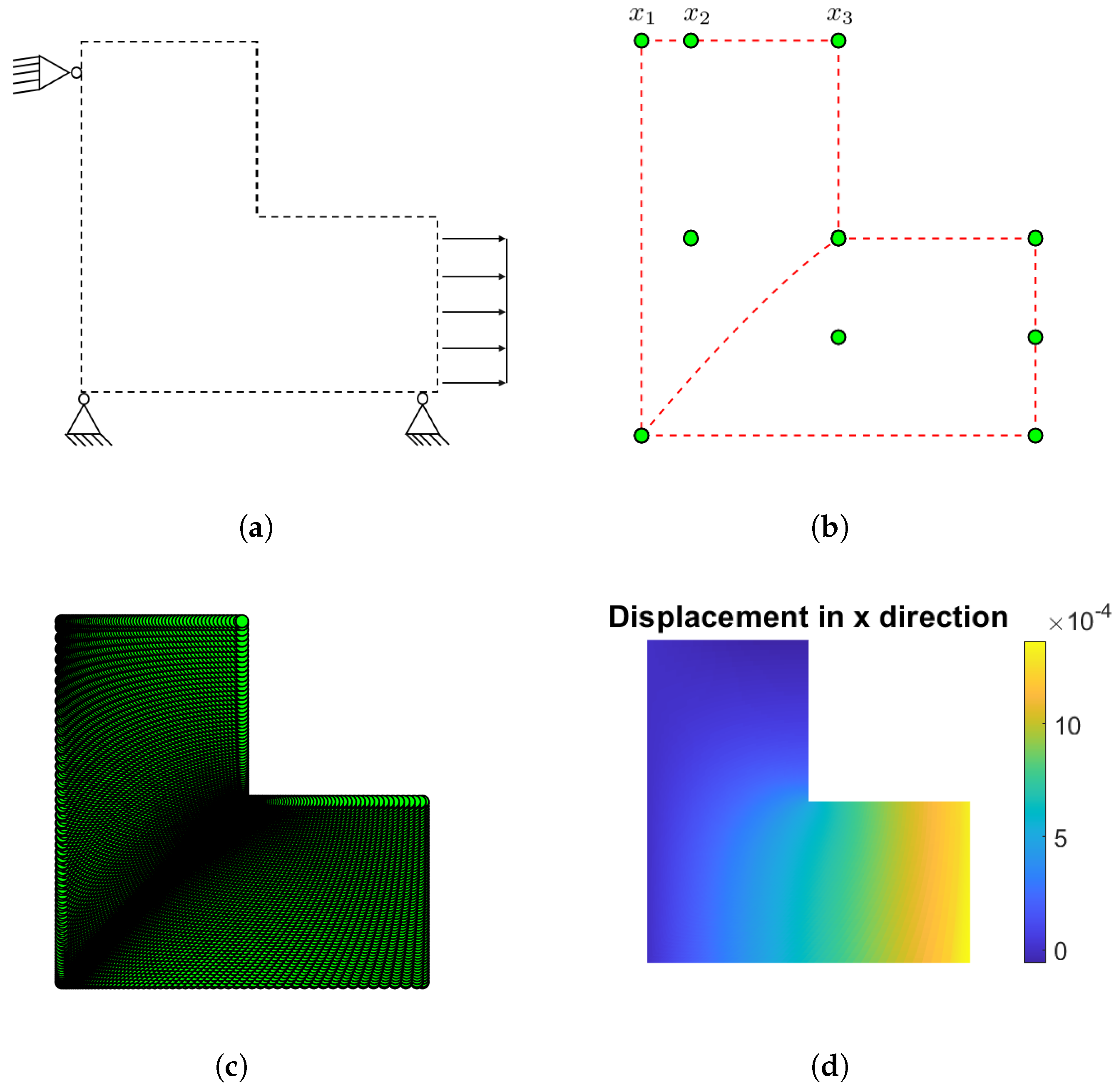
Figure 4.
L-shape under uniaxial loading. Figure 4(a) shows the mechanical problem: the lower right edge of the structure is subjected to a uniform tensile load, while the left and lower edges are restrained in the x and y directions, respectively. Figure 4(b) shows how the control points that define the geometry are distributed. Figure 4(c) shows the initial configuration of the domain, and, Figure 4(d) illustrates the displacement in the x direction, represented by a contour plot.
The goal is to minimize the total volume while ensuring that the average horizontal displacement matches a prescribed target. The optimization problem is therefore formulated as follows:
where:
- is the total volume of the generated structure,
- is the average horizontal displacement on the right boundary ,
- is the target displacement,
- is a regularization coefficient.
Each evaluation of requires solving an isogeometric elasticity FE problem:
where is the stiffness matrix depending on the geometry modified by , and is the associated displacement field. This formulation guarantees mechanical consistency via the imposed equilibrium, while the volume term, although approximate, plays a regularizing role, guiding the solution towards more compact forms without explicitly restricting the space of admissible designs.
To initiate the optimization process, an initial DoE comprising 12 samples was generated using Latin hypercube sampling (LHS). The admissible set is defined by the lower and upper bounds . To evaluate the acquisition function at each iteration, a Monte Carlo sampling of points was extracted from the design space. The hyperparameters of the proposed optimization algorithm were established as follows: the quantile threshold was used in the definition of the probability of improvement, and the scale coefficient . Furthermore, to divide the DoE into ‘good’ and ‘bad’ subsets, response values were taken to construct a priori distributions representing the promising and unpromising regions of the design space.
Figure 5 shows the evolution of the volume throughout the optimization process. The initial volume corresponds to the original L-shaped design. The first 20 iterations were performed using the proposed HSBO method. During this phase, the volume was progressively reduced, especially in the first iterations. Once these 20 iterations were completed, the best solution obtained with HSBO, as well as the trained Gaussian surrogate, were taken as the starting point and surrogate objective functions for a local gradient-based optimization procedure, implemented using Matlab’s fmincon function. The algorithm used by fmincon (by default, interior-point) was configured with standard tolerance settings. This second stage successfully converged towards the optimum, achieving a total volume reduction of approximately 30% compared to the initial design. In terms of computational cost, HSBO used 12 functional evaluations to build the DoE, followed by 20 more evaluations during the iterative process, for a total of 32 evaluations. Since fmincon was applied to the Gaussian Process surrogate, no additional functional evaluation was required during this refinement step. Overall, the entire process involved 32 functional evaluations. This hybrid approach illustrates HSBO’s versatility and its efficiency in training the Gaussian surrogate with scarce data and with high accuracy around the region surrounding the optimum.
Figure 6 shows the results of the optimized L. Figure 6(a) shows the final positions of the three control points that act as design variables. Their vertical displacements generate the diagonal notch responsible for the volume reduction. Figure 6(b) shows the resulting refined NURBS mesh, which has uniform quality elements and a deformation field without local concentrations, confirming the mechanical consistency of the optimized shape. Figure 6(c) shows the contour of the horizontal displacement , which exhibits a nearly linear gradient between the embedded edge and the right edge; the uniform color band on confirms that the average displacement reaches the target with minimal dispersion.
5. Discussion
In this article, we have presented HSBO, a version of BO that combines Bayesian-Hilbertian UQ modeling techniques within the framework of Bayesian optimisation. The role of HA is the construction of structured performance priors over the search space, identifying regions of promising performance to guide the Bayesian enrichment process. We have performed several synthetic tests to evaluate the behavior of this method, revealing competitive performance in selected cases.
The numerical tests, carried out on various test functions with varying characteristics and dimensions, reveal that the proposed method provides a systematic framework for prior construction that can enhance classical BO performance when problem structure aligns with the selected parametric family. The improved performance can manifest as increased success rate, faster convergence, or closer proximity to the optimum on a fixed budget, with respect to SBO. Even in situations where the global minimum is not identified, the method converges towards regions very close to the optimum, which represents an excellent starting point for gradient-based refinement methods.
This latter property has been particularly useful in the structural shape optimization application presented, where the aim was to minimize the volume of a solid, initially an L-shaped plate. The Bayesian-Hilbertian approach made it possible to identify, with only 20 iterations, a restricted region of the search space enclosing the optimal solution. This region, and the associated metamodel trained with the selected points, served as the initial basis for a gradient-based algorithm to refine the search, yielding an accurate solution with no additional evaluation of the underlying expensive objective function.
This approach is particularly relevant for engineering problems where expert priors are difficult to define, yet initial design data can be obtained with reasonable effort. In such cases, constructing a small exploratory design of experiments (DoE) is worthwhile, as it enables a principled, data-driven initialization of the optimization process with minimal reliance on human bias.
Future lines of inquiry include: the investigation of the impact of explicit modeling of dependencies between data when constructing the priors; sensitivity analysis of the hyperparametes involved, particularly and ; consideration of other surrogates. Additionally, two promising complements of this work would include the manipulation of the priors to integrate constrained optimization into this framework, and guided biasing of the priors to boost convergence speed.
Abbreviations
The following abbreviations are used in this manuscript:
| BO | Bayesian Optimization |
| Gaussian Process | |
| BOPrO | Bayesian optimization with a prior for the optimum |
| BOA | Bayesian Optimization Algorithm |
| SBO | Standart Bayesian Optimization |
| TPE | Tree-structured Parzen Estimator |
| CDF | cumulative distribution function |
| probability density function | |
| HSBO | Data-Driven Prior Construction in Hilbert Spaces for Bayesian Optimization |
| DoE | Initial design of experiments |
| SR | Simple Regret |
Appendix A. Description of test functions
Table A1.
Test cases
| Function | Dimension | Design Space | Minimun | Target |
|---|---|---|---|---|
| (F1) Gramacy & Lee (2012) | ||||
| 1 | -0.86901 | -0.8256 | ||
| (F2) Cross-in-Tray | ||||
| 2 | -2.06261 | -1.9595 | ||
| (F3) Branin | ||||
| 2 | 0.397887 | 0.4178 | ||
| (F4) Hartmann 3-Dimensional | ||||
| 3 | -3.86278 | -3.6696 | ||
| (F5) Sum of Different Powers Function | ||||
| 4 | 0 | 0.001 | ||
| (F6) Hartmann 6-Dimensional | ||||
| 6 | -3.32237 | -3.1563 |
Appendix B. Mean of Simple Regret
The Gramacy & Lee function (Figure A1(a)), shows that the configuration based on Pearson’s distribution stands out for its rapid convergence, achieving the lowest simple regret values in fewer iterations than the baseline and the other variants of the proposed method.
Figure A1.
Log-scale simple regret mean versus iteration count for various benchmark functions. Results correspond to the average of 10 runs using random initial DoE.
Figure A1.
Log-scale simple regret mean versus iteration count for various benchmark functions. Results correspond to the average of 10 runs using random initial DoE.
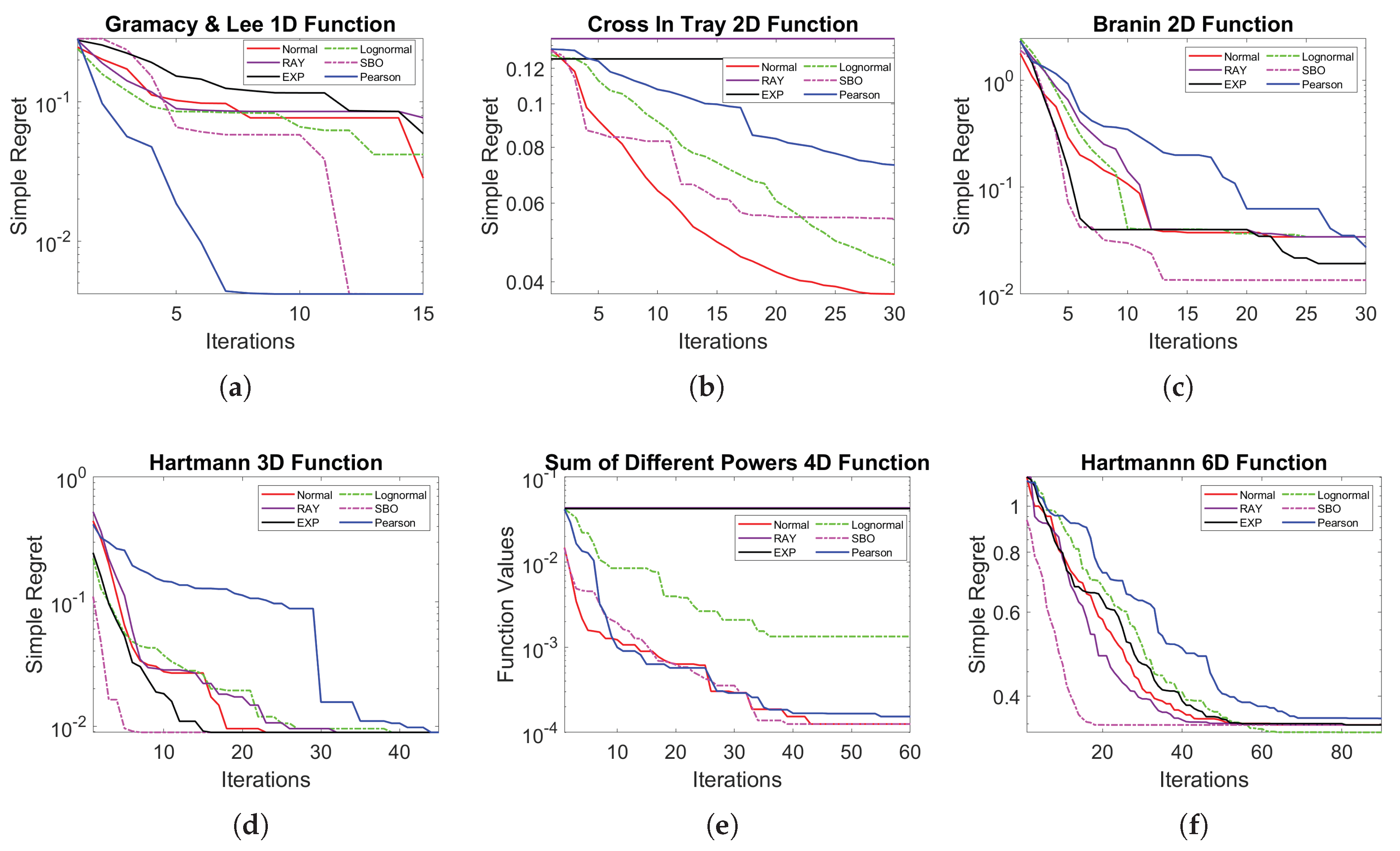
When analyzing the Cross-in-Tray function (Figure A1(b)), the normal and lognormal distributions offer clearly superior performance, achieving a considerably lower simple regret than the other methods, including SBO.
Regarding the Branin function (Figure A1(c)), all methods tend to converge towards similar levels of simple regret during the first iterations. However, it can be observed that the baseline presents the fastest and most stable convergence, reaching a very low level of regret from approximately the tenth iteration onwards.
Turning to the Hartmann 3D function (Figure A1(d)), the SBO method shows the fastest convergence, reaching the lowest simple regret values in just a few iterations.
With the 4D version of the Sum of Different Powers function (Figure A1(e)), the configurations based on the normal and Pearson distributions converge slightly faster towards the target value of . However, the difference with respect to SBO is not significant, since it also converges to the same level in a similar number of iterations.
Finally, the results for the Hartmann 6D function (Figure A1(f)), it can be seen that although SBO shows very rapid convergence in the first iterations, its progress soon stabilises, while the lognormal configuration continues to improve gradually until it achieves the best overall performance.
References
- Jones, D.R.; Schonlau, M.; Welch, W.J. Efficient global optimization of expensive black-box functions. Journal of Global optimization 1998, 13, 455–492. [CrossRef]
- Regis, R.G. Stochastic radial basis function algorithms for large-scale optimization involving expensive black-box objective and constraint functions. Computers & Operations Research 2011, 38, 837–853. [CrossRef]
- Kumagai, W.; Yasuda, K. Black-box optimization and its applications. Innovative systems approach for facilitating smarter world 2023, pp. 81–100.
- Ghanbari, H.; Scheinberg, K. Black-box optimization in machine learning with trust region based derivative free algorithm. arXiv preprint arXiv:1703.06925 2017.
- Pardalos, P.M.; Rasskazova, V.; Vrahatis, M.N.; et al. Black box optimization, machine learning, and no-free lunch theorems; Vol. 170, Springer, 2021.
- Abreu de Souza, F.; Crispim Romão, M.; Castro, N.F.; Nikjoo, M.; Porod, W. Exploring parameter spaces with artificial intelligence and machine learning black-box optimization algorithms. Physical Review D 2023, 107, 035004. [CrossRef]
- Calvel, S.; Mongeau, M. Black-box structural optimization of a mechanical component. Computers & Industrial Engineering 2007, 53, 514–530. [CrossRef]
- Lainé, J.; Piollet, E.; Nyssen, F.; Batailly, A. Blackbox optimization for aircraft engine blades with contact interfaces. Journal of Engineering for Gas Turbines and Power 2019, 141, 061016. [CrossRef]
- Thalhamer, A.; Fleisch, M.; Schuecker, C.; Fuchs, P.F.; Schlögl, S.; Berer, M. A black-box optimization strategy for customizable global elastic deformation behavior of unit cell-based tri-anti-chiral metamaterials. Advances in Engineering Software 2023, 186, 103553. [CrossRef]
- Wu, J.; Chen, X.Y.; Zhang, H.; Xiong, L.D.; Lei, H.; Deng, S.H. Hyperparameter optimization for machine learning models based on Bayesian optimization. Journal of Electronic Science and Technology 2019, 17, 26–40.
- Cho, H.; Kim, Y.; Lee, E.; Choi, D.; Lee, Y.; Rhee, W. Basic enhancement strategies when using Bayesian optimization for hyperparameter tuning of deep neural networks. IEEE access 2020, 8, 52588–52608. [CrossRef]
- Do, B.; Zhang, R. Multi-fidelity Bayesian optimization in engineering design. arXiv preprint arXiv:2311.13050 2023.
- Frazier, P.I.; Wang, J. Bayesian optimization for materials design. Information science for materials discovery and design 2016, pp. 45–75.
- Humphrey, L.; Dubas, A.; Fletcher, L.; Davis, A. Machine learning techniques for sequential learning engineering design optimisation. Plasma Physics and Controlled Fusion 2023, 66, 025002. [CrossRef]
- Brochu, E.; Cora, V.M.; De Freitas, N. A tutorial on Bayesian optimization of expensive cost functions, with application to active user modeling and hierarchical reinforcement learning. arXiv preprint arXiv:1012.2599 2010.
- Mockus, J. Application of Bayesian approach to numerical methods of global and stochastic optimization. Journal of Global Optimization 1994, 4, 347–365. [CrossRef]
- Frazier, P.I. A tutorial on Bayesian optimization. arXiv preprint arXiv:1807.02811 2018.
- Wilson, A.G.; Dann, C.; Lucas, C.; Xing, E.P. The human kernel. Advances in neural information processing systems 2015, 28.
- Xu, W.; Adachi, M.; Jones, C.N.; Osborne, M.A. Principled bayesian optimisation in collaboration with human experts. arXiv preprint arXiv:2410.10452 2024.
- Souza, A.; Nardi, L.; Oliveira, L.B.; Olukotun, K.; Lindauer, M.; Hutter, F. Bayesian optimization with a prior for the optimum. In Proceedings of the Machine Learning and Knowledge Discovery in Databases. Research Track: European Conference, ECML PKDD 2021, Bilbao, Spain, September 13–17, 2021, Proceedings, Part III 21. Springer, 2021, pp. 265–296.
- de Cursi, E.S. Uncertainty Quantification with R; Springer, 2024.
- Shahriari, B.; Swersky, K.; Wang, Z.; Adams, R.P.; De Freitas, N. Taking the human out of the loop: A review of Bayesian optimization. Proceedings of the IEEE 2015, 104, 148–175. [CrossRef]
- Ben Yahya, A.; Ramos Garces, S.; Van Oosterwyck, N.; De Boi, I.; Cuyt, A.; Derammelaere, S. Mechanism design optimization through CAD-based Bayesian optimization and quantified constraints. Discover Mechanical Engineering 2024, 3, 21. [CrossRef]
- Surjanovic, S.; Bingham, D. Virtual Library of Simulation Experiments: Test Functions and Datasets. https://www.sfu.ca/~ssurjano/optimization.html, 2013.
- Bergstra, J.; Bardenet, R.; Bengio, Y.; Kégl, B. Algorithms for hyper-parameter optimization. Advances in neural information processing systems 2011, 24.
- de Cursi, E.S.; Fabro, A. On the Collaboration Between Bayesian and Hilbertian Approaches. In Proceedings of the International Symposium on Uncertainty Quantification and Stochastic Modeling. Springer, 2023, pp. 178–189.
- Bassi, M.; Souza de Cursi, J.E.; Ellaia, R. Generalized Fourier Series for Representing Random Variables and Application for Quantifying Uncertainties in Optimization. In Proceedings of the 3rd International Symposium on Uncertainty Quantification and Stochastic Modeling, 2016. [CrossRef]
- De Cursi, E.S.; Sampaio, R. Uncertainty quantification and stochastic modeling with matlab; Elsevier, 2015.
- AV, A.K.; Rana, S.; Shilton, A.; Venkatesh, S. Human-AI collaborative Bayesian optimisation. Advances in Neural Information Processing Systems 2022, 35, 16233–16245.
- Vakili, S.; Bouziani, N.; Jalali, S.; Bernacchia, A.; Shiu, D.s. Optimal order simple regret for Gaussian process bandits. Advances in Neural Information Processing Systems 2021, 34, 21202–21215.
- Nguyen, V.P.; Anitescu, C.; Bordas, S.P.; Rabczuk, T. Isogeometric analysis: an overview and computer implementation aspects. Mathematics and Computers in Simulation 2015, 117, 89–116. [CrossRef]
| 1 | The numerical model is based on the open-source code MIGFEM by Vinh Phu Nguyen (Johns Hopkins University / Monash University), available on GitHub. This MATLAB code implements linear isogeometric analysis (IGA) for 1D, 2D, and 3D elasticity problems, including refinement and Bézier extraction. |
Figure 2.
Illustrative example of the optimisation process of the proposed method. (a) shows the true function () and DoE split into good () and bad points () for prior construction, (b) shows prior densities and , constructed via our data-driven procedure, (c) shows the mean of the surrogate model with the associated uncertainty and the next evaluation point, (d) shows model-based probabilities and of being a good or bad point, (e) shows weighted pseudo-posterior and , and (f) shows EI acquisition function with the selected next evaluation point.
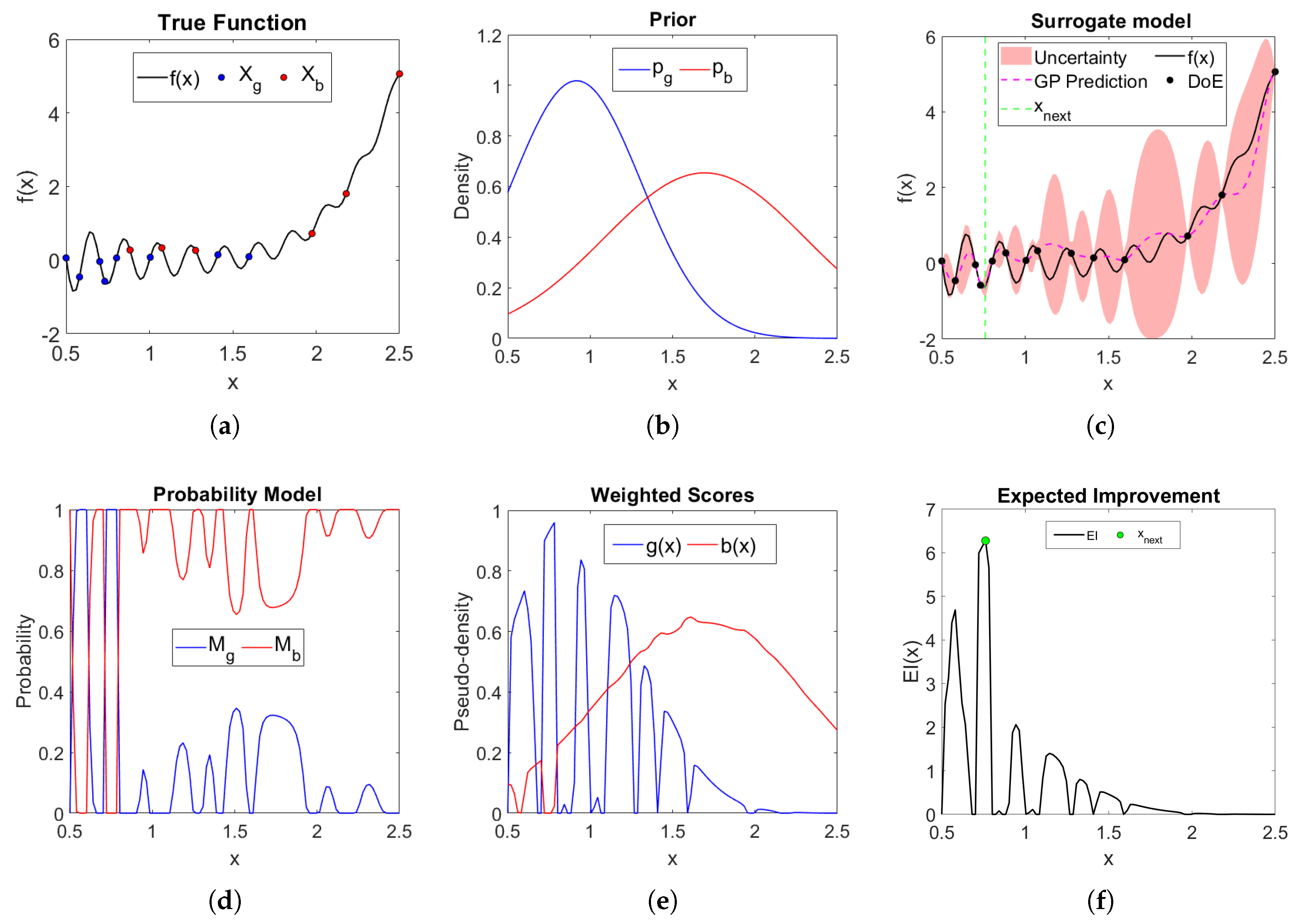
Figure 3.
Box plots illustrate the performance at the last iteration after 10 runs—each starting from a random DoE—of the proposed method under five different prior distributions (normal, log-normal, Rayleigh, exponential, and Pearson), with SBO used as the baseline. Results are reported for six benchmark functions. The vertical axis shows the relative error with respect to the global minimum, except for case 3(e), whose optimum is zero; there, the objective-function value itself is plotted.
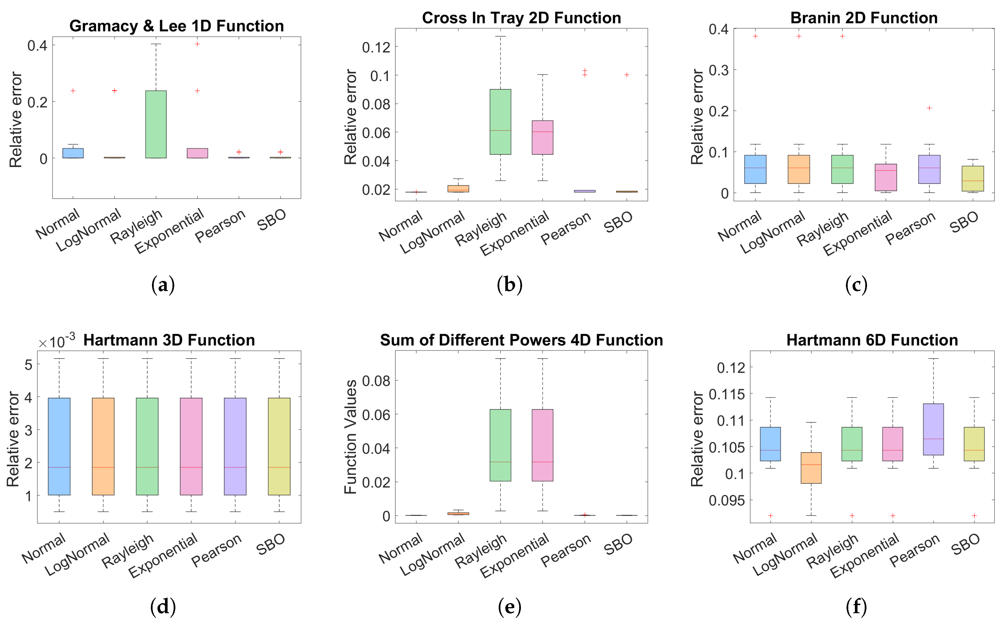
Figure 5.
History of the objective function of volume for the L-shaped design problem. Volume is drastically reduced in the first iterations of the design and stabilizes after a reduction of approximately 30% from the initial design.
Figure 5.
History of the objective function of volume for the L-shaped design problem. Volume is drastically reduced in the first iterations of the design and stabilizes after a reduction of approximately 30% from the initial design.
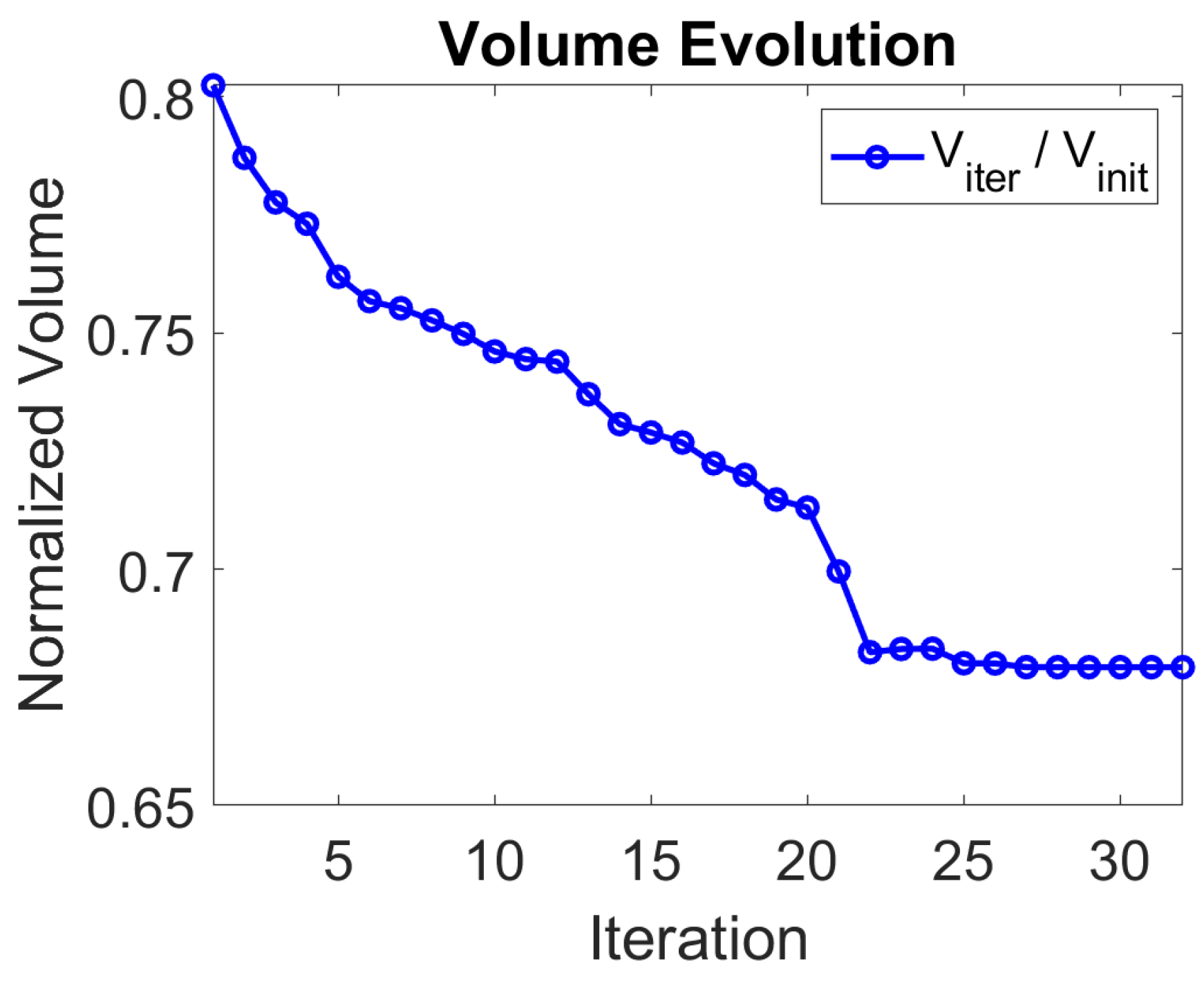
Figure 6.
Distribution of the displacement component in the x-direction for the optimal shape design.
Figure 6.
Distribution of the displacement component in the x-direction for the optimal shape design.
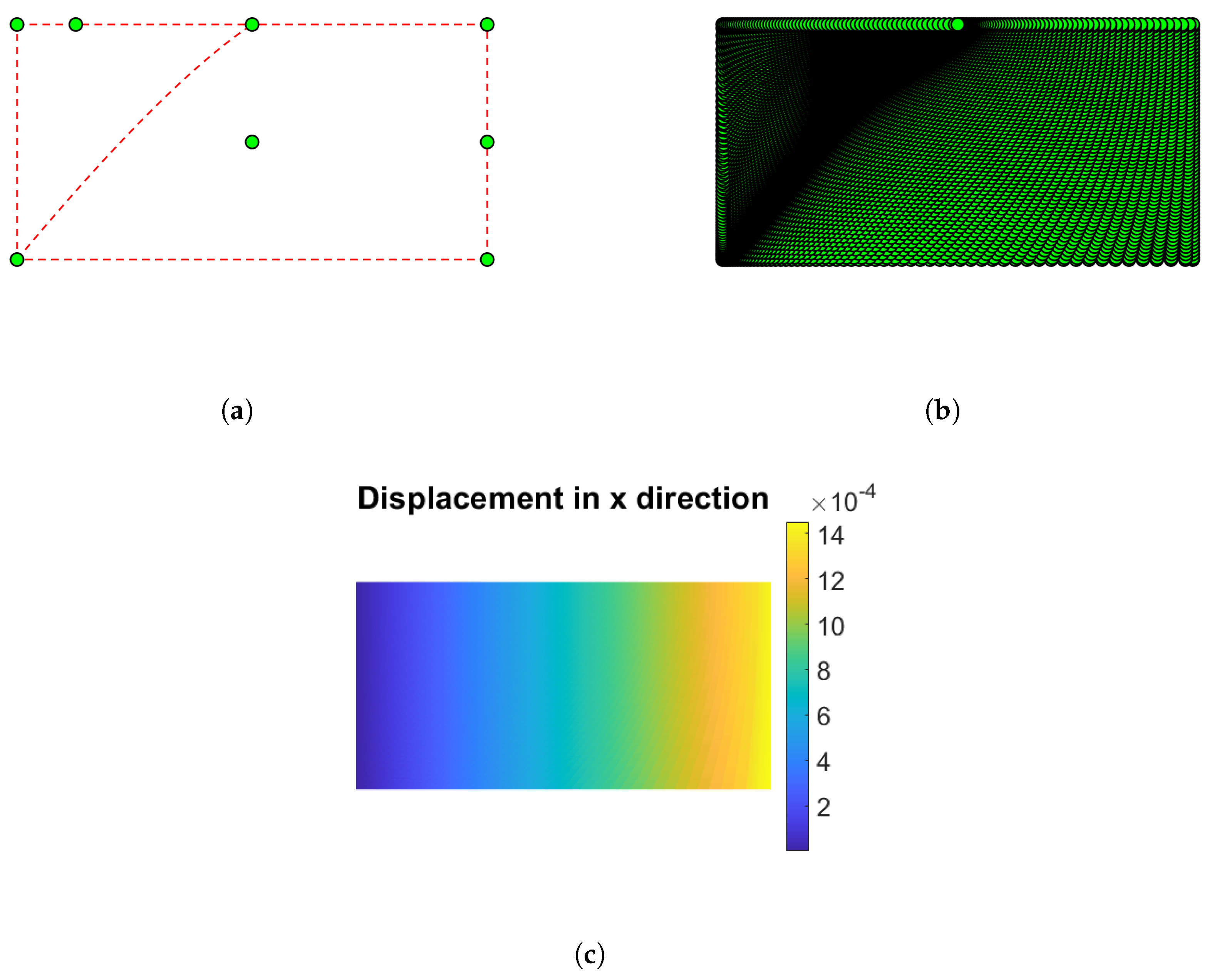
Table 2.
Performance at Final Iteration () over 10 Runs: Cross-in-tray 2D Function
| Method | Min () | Max () | Mean () | Std() | Success rate ( target) |
|---|---|---|---|---|---|
| SBO (baseline) | -2.0626 | -1.8894 | -2.0447 | 9/10 | |
| HSBO with normal prior | -2.0626 | -2.0620 | -2.0625 | 10/10 | |
| HSBO with log-normal prior | -2.0626 | -2.0426 | -2.0564 | 10/10 | |
| HSBO with exponential prior | -2.0456 | -1.8891 | -1.9740 | 7/10 | |
| HSBO with Rayleigh prior | -2.0456 | -1.8327 | -1.9601 | 6/10 | |
| HSBO with Pearson prior | -2.0626 | -1.8833 | -2.0270 | 8/10 |
Table 3.
Performance at Final Iteration () over 10 Runs: Branin 2D Function
| Method | Min () | Max () | Mean () | Std() | Success rate ( target) |
|---|---|---|---|---|---|
| SBO (baseline) | 0.3980 | 0.4303 | 0.4114 | 6/10 | |
| HSBO with normal prior | 0.3980 | 0.5495 | 0.4322 | 3/10 | |
| HSBO with log-normal prior | 0.3980 | 0.5495 | 0.4322 | 3/10 | |
| HSBO with exponential prior | 0.3980 | 0.4449 | 0.4171 | 4/10 | |
| HSBO with Rayleigh prior | 0.3980 | 0.5495 | 0.4322 | 3/10 | |
| HSBO with Pearson prior | 0.3980 | 0.4801 | 0.4252 | 3/10 |
Table 4.
Performance at Final Iteration () over 10 Runs: Hartmann 3D Function
| Method | Min () | Max () | Mean () | Std() | Success rate ( target) |
|---|---|---|---|---|---|
| SBO (baseline) | -3.8609 | -3.8428 | -3.8539 | 10/10 | |
| HSBO with normal prior | -3.8609 | -3.8428 | -3.8539 | 10/10 | |
| HSBO with log-normal prior | -3.8609 | -3.8428 | -3.8539 | 10/10 | |
| HSBO with exponential prior | -3.8609 | -3.8428 | -3.8539 | 10/10 | |
| HSBO with Rayleigh prior | -3.8609 | -3.8428 | -3.8539 | 10/10 | |
| HSBO with Pearson prior | -3.8609 | -3.8428 | -3.8539 | 10/10 |
Table 5.
Performance at Final Iteration () over 10 Runs: Sum of Different Powers Function
| Method | Min () | Max () | Mean () | Std() | Success rate ( target) |
|---|---|---|---|---|---|
| SBO (baseline) | 10/10 | ||||
| HSBO with normal prior | 10/10 | ||||
| HSBO with log-normal prior | 5/10 | ||||
| HSBO with exponential prior | - | ||||
| HSBO with Rayleigh prior | - | ||||
| HSBO with Pearson prior | 10/10 |
Table 6.
Performance at Final Iteration () over 10 Runs: Hartmann 6D Function
| Method | Min () | Max () | Mean () | Std() | Success rate ( target) |
|---|---|---|---|---|---|
| SBO (baseline) | -3.0166 | -2.9428 | -2.9742 | - | |
| HSBO with normal prior | -3.0166 | -2.9428 | -2.9740 | - | |
| HSBO with log-normal prior | -3.0166 | -2.9583 | -2.9864 | - | |
| HSBO with exponential prior | -3.0166 | -2.9428 | -2.9742 | - | |
| HSBO with Rayleigh prior | -3.0166 | -2.9428 | -2.9742 | - | |
| HSBO with Pearson prior | -2.9871 | -2.9184 | -2.9632 | - |
Disclaimer/Publisher’s Note: The statements, opinions and data contained in all publications are solely those of the individual author(s) and contributor(s) and not of MDPI and/or the editor(s). MDPI and/or the editor(s) disclaim responsibility for any injury to people or property resulting from any ideas, methods, instructions or products referred to in the content. |
© 2025 by the authors. Licensee MDPI, Basel, Switzerland. This article is an open access article distributed under the terms and conditions of the Creative Commons Attribution (CC BY) license (http://creativecommons.org/licenses/by/4.0/).
Copyright: This open access article is published under a Creative Commons CC BY 4.0 license, which permit the free download, distribution, and reuse, provided that the author and preprint are cited in any reuse.


