Tensor Formalism for Rotating Bodies in Multidimensional Euclidian Space

1. Rotation of Rigid Bodies

The concepts of torque, angular momentum, and moment of inertia, which are fundamental to the description of rotational motions, can be regarded as analogs to the concepts of force, linear momentum, and mass, which are fundamental to linear motions. The interconnectedness of these physical quantities is predicated on the fundamental law of dynamics, a foundational principle that governs rotational motion. The rigid body can be used as a model for a piece of ordinary, solid matter; the internal degrees of freedom (such as vibrations) are neglected. This approach offers a distinct pedagogical advantage, whereby many observations concerning the rigid body appear to stem from statements about systems of mass points. However, it is imperative to acknowledge that the transition to continuous mass distributions necessitates additional fundamental assumptions. In order to transition from the mechanics of mass points, the following statement can be made: It is evident that a system of mass points, under specific conditions, will demonstrate a tendency to behave like a rigid body. These actions are contingent upon the system's mutual 4D-spatial distances remaining constant over time. The rotational movements of rigid bodies in Euclidean space are defined by two key parameters: their instantaneous angular velocity and angular momentum (Hestenes, 2002). A rigid body has several degrees of freedom, in ${\mathbb{R}}^N$ there are $N$ degrees of freedom of the translations and $N_{\omega }=N·\left(N-1\right)/2$ of rotations. To describe the movement, we consider an inertial system (in where Newton’s axioms apply) and a body-fixed system (in which we calculate inertia tensor):

Body-fixed coordinate system $BS$: $x_1,..,x_N$ and $e_1,..,e_N$.

Inertial coordinate system$IS:$ $X_1,..,X_N$ and $E_1,..,E_N$.

The body-fixed $BS$ may move with the (generally time-dependent) angular velocity relative to the $IS$. A rigid body is defined as a body whose constituents invariably maintain constant distances between each other, signifying that they are rigidly bound to one another. A rigid body is a system of a certain number of mass points $m_{\left(\nu \right)}$. The positions of the mass points ${\mathit{r}}_{\left(\nu \right)}$ and ${\mathit{r}}_{\left(\varsigma \right)}$ have been established as fixed in $BS$. Consequently, the relative distances ${\mathit{r}}_{(\varsigma ,\nu )} = {\mathit{r}}_{\left(\varsigma \right)}-{\mathit{r}}_{\left(\nu \right)}$ remain constant in course of motion.

2. Rotations in 3D

2.1. Vectors of Angular Moment and Rotation

For the beginning, we briefly account the standard notations for the dynamics of rigid bodies in vector form (Krey & Owen, 2007). The angular momentum, $\overrightarrow{\mathbb{L}}$ and the external torque $\overrightarrow{\mathbb{m}}$ are the vectors of dimension $N=3$. In the context of rotational motions, it can be posited that torque is equivalent to the change in angular momentum, $\overrightarrow{\mathbb{L}}$ over a specified interval of time for a given external torque $\overrightarrow{\mathbb{m}}$ (Hestenes, 2002):

$d\overrightarrow{\mathbb{L}}/dt=\overrightarrow{\mathbb{m}}$.

Euler rotational vector is introduced as generalized coordinates for the rotational motion of a rigid body:

$\overrightarrow{\mathsf{\Omega }}=⟦\begin{array}{c}{\mathsf{\Omega }}_1\\ {\mathsf{\Omega }}_2\\ {\mathsf{\Omega }}_3\end{array}⟧$.

The inertia of the body during rotation is commonly described in 3D-Space by the tensor:

$\stackrel{⃡}{\mathbb{I}}=⟦\begin{array}{ccc}{\mathbb{I}}_{11}& {\mathbb{I}}_{12}& {\mathbb{I}}_{13}\\ {\mathbb{I}}_{12}& {\mathbb{I}}_{22}& {\mathbb{I}}_{23}\\ {\mathbb{I}}_{13}& {\mathbb{I}}_{23}& {\mathbb{I}}_{33}\end{array}⟧$.

The angular momentum is the product of inertia matrix (3) to rotational vector (2):

$\overrightarrow{\mathbb{L}}=⟦\begin{array}{c}{\mathbb{L}}_1\\ {\mathbb{L}}_2\\ {\mathbb{L}}_3\end{array}⟧=⟦\begin{array}{c}{\mathbb{I}}_{11}{\mathsf{\Omega }}_1+{\mathbb{I}}_{12}{\mathsf{\Omega }}_2+{\mathbb{I}}_{13}{\mathsf{\Omega }}_3\\ {\mathbb{I}}_{12}{\mathsf{\Omega }}_1+{\mathbb{I}}_{22}{\mathsf{\Omega }}_2+{\mathbb{I}}_{23}{\mathsf{\Omega }}_3\\ {\mathbb{I}}_{13}{\mathsf{\Omega }}_1+{\mathbb{I}}_{23}{\mathsf{\Omega }}_2+{\mathbb{I}}_{33}{\mathsf{\Omega }}_3\end{array}⟧$, $\overrightarrow{\mathbb{m}}=⟦\begin{array}{c}{\mathbb{m}}_1\\ {\mathbb{m}}_2\\ {\mathbb{m}}_3\end{array}⟧$.

The form of the inertia tensor (3) is dependent on the chosen coordinate system $BS$. However, a system of principal axes can always be found in which the tensor has a diagonal form. We consider two different body-fixed Cartesian systems, $BS$ and $\widetilde{BS}$ , the are rotated relative to each other; however, they should have the same origin. The transformation of the inertia tensor to the principal axes of $\widetilde{BS}$ is considered herein, employing matrix notation. Now, the symmetric matrix (3) can be diagonalized by an orthogonal transformation:

$\stackrel{⃡}{\mathbb{I}}=⟦\begin{array}{ccc}{\mathbb{I}}_I& 0& 0\\ 0& {\mathbb{I}}_{II}& 0\\ 0& 0& {\mathbb{I}}_{III}\end{array}⟧$, $\overrightarrow{\mathbb{L}}=⟦\begin{array}{c}{\mathbb{I}}_I{\mathsf{\Omega }}_1\\ {\mathbb{I}}_{II}{\mathsf{\Omega }}_2\\ {\mathbb{I}}_{III}{\mathsf{\Omega }}_3\end{array}⟧$.

The coordinate system, in which the matrix of moments of inertia is diagonal is called the principal axis system $\widetilde{BS}$. The diagonal elements ${\mathbb{I}}_I,{\mathbb{I}}_{II},{\mathbb{I}}_{III}$, are the moments of inertia with respect to the rotation around the axes of $\widetilde{BS}$. The principal moments of inertia ${\mathbb{I}}_I,{\mathbb{I}}_{II},{\mathbb{I}}_{III}$ are positive.

2.2. Euler's Equations in Vector Form

In the context of a spatially fixed system, the inertia tensor is contingent on the instantaneous orientation of the body. For linear motion, this would approximately correspond to a position-dependent mass, if we disregard the fact that, in this context, it is not possible to consider that the function of the orientation is a scalar. It is possible to establish a constant value for this function by considering the movement not in the space-fixed system but in the body-fixed system. The transition between the two reference systems can be facilitated by the Coriolis theorem (Landau & Lifshitz, 1976). The components of Euler’s equations in four-dimensional space read as:

${\displaystyle \frac{d\overrightarrow{\mathbb{L}}}{dt}}+\overrightarrow{\mathsf{\Omega }}\times \overrightarrow{\mathbb{L}}=\overrightarrow{\mathbb{m}}$.

The components of the Eq. (6) are as follows:

${\mathbb{I}}_I{\displaystyle \frac{d{\mathsf{\Omega }}_1}{dt}}+\left({\mathbb{I}}_{III}-{\mathbb{I}}_{II}\right){\mathsf{\Omega }}_2{\mathsf{\Omega }}_3={\mathbb{m}}_1,$${\mathbb{I}}_{II}{\displaystyle \frac{d{\mathsf{\Omega }}_2}{dt}}+\left({\mathbb{I}}_I-{\mathbb{I}}_{III}\right){\mathsf{\Omega }}_3{\mathsf{\Omega }}_1={\mathbb{m}}_2$,

${\mathbb{I}}_{III}{\displaystyle \frac{d{\mathsf{\Omega }}_3}{dt}}+\left({\mathbb{I}}_{II}-{\mathbb{I}}_I\right){\mathsf{\Omega }}_1{\mathsf{\Omega }}_2={\mathbb{m}}_3$.

The Eq. (7),(8),(9) are the classical Euler equations (Landau & Lifshitz, 1976), (Krey & Owen, 2007). The vector representation is possible because the number of sub-diagonal elements is 3, which is identical to the number of diagonal elements of the matrix (5).

3. Arbitrary Degrees of Freedom

3.1. Tensor Description of the Rotations

In an arbitrary number of spatial dimensions, the mechanical characteristics in rotational dynamics are represented by bivectors (antisymmetric rank-2 tensors) (Cayley, 1846), (Ten Bosch, 2020), (Parker, 2024). The rotation velocity is represented by an antisymmetric tensor of rank 2:

$\begin{array}{cc}\mathit{\omega }=⟦{\omega }_{kl}⟧,& {\omega }_{kl}=-{\omega }_{lk}\end{array}$.

The elementary rotation of the body occurs over a specific axis. The axis of rotation is defined as being normal to the plane of rotation. The plane of rotation is defined by the two vectors that belong to it, namely, $k$ and $l$ [1]. The elementary rotation ${\omega }_{kl}$ is thus characterized by the indices of both vectors $k$ and $l$ . The angular velocity (10) does not change if chooses a different origin for $KS$. The orientation of the body-fixed system relative to the $IS$ is determined by the degrees of freedom. The non-zero elements of matrix (10) can be described as generalized coordinates. Their number is equal to:

$N_{\omega }={\displaystyle \frac{N\left(N-1\right)}{2}}.$Take a frame of reference $BS$ associated with a solid body, and consider a vector $\mathbb{T}=⟦{\mathbb{T}}_i⟧$ going from its origin to some point of the body. Obviously, in the body-fixed coordinate system $BS$ this vector will appear constant. However, an observer located in an inertial frame of reference $IS$, will consider that components of this vector $\mathbb{t}$ change during the motion of the body. Let us consider the increments that the components of an arbitrary vector or tensor $\mathbb{T}$ receive during time$dt$. In the reference frame associated with the body $BS$, they will differ from the corresponding increments in the inertial coordinate system $IS$. The relationship between the two increments of vector $\mathbb{T}$ can be obtained by a simple physical reasoning. The only difference between them is due to the rotation of the system $BS$ associated with the body. Symbolically it can be written as follows:

$d\mathbb{t}=d\mathbb{T}+{d\mathbb{T}}_{rotation}$.

Now consider the vector associated with the system $BS$. As the body rotates, the components of this vector do not change (from the point of view of the observer associated with the body), i.e., they remain constant with respect to the axes of the reference frame $BS$ associated with the body. In this case the only contribution to $d\mathbb{t}$ will be ${d\mathbb{T}}_{rotation}$ due to the rotation of the body. But since the vector is associated with the body, it rotates in the opposite direction and, from the point of view of a stationary observer. in 4D-space, the increment is equal to:

${\left({d\mathbb{T}}_{rotation}\right)}_l={ϵ}_l^{ijk}{d\mathsf{\Omega }}_{ij}{\mathbb{T}}_k$.

In the 4D-space, the Levi-Civita-pseudo-tensors $\mathit{ϵ}=⟦{ϵ}_l^{ijk}⟧$ are of rank 4. It is imperative that the rank of the Levi-Civita pseudo-tensors align with the dimension of space $N$. The change of an arbitrary vector in a fixed frame of reference $IS$ is determined by the sum of two components:

${d\mathbb{t}}_l={d\mathbb{T}}_l+{ϵ}_l^{ijk}{d\mathsf{\Omega }}_{ij}{\mathbb{T}}_k$.

The relationship between the rates of change of the vector $\mathbb{t}=⟦{\mathbb{t}}_l⟧$ from the point of view of the two observers, is obtained by dividing (4.81) by the time differential $dt$:

${\displaystyle \frac{\mathrm{d}{\mathbb{t}}_l}{dt}}={\displaystyle \frac{\mathrm{d}{\mathbb{T}}_l}{dt}}+{ϵ}_l^{ijk}{\mathsf{\omega }}_{ij}{\mathbb{T}}_k$.

Here ${\mathsf{\omega }}_{\mathit{i}\mathit{j}}$ is the instantaneous angular velocity (10):

${\mathsf{\omega }}_{ij}\stackrel{\scriptscriptstyle\mathrm{def}}{=}{\displaystyle \frac{{d\mathsf{\Omega }}_{ij}}{dt}}$.

The previously defined tensor $\mathsf{\omega }=⟦{\mathsf{\omega }}_{ij}⟧$ signifies the angular velocity of the rotation of the system $BS$ relative to the inertial reference frame $IS$. The equation allows us to modify the equations of motion so that they are valid in a rotating non-inertial frame of reference.

Equality (15) should not be regarded as a formula relating to any particular vector or tensor, but rather as an equation of the of the transformation of the time derivative when moving from one coordinate system to another. Consider for example an arbitrary tensor ${\mathbb{T}}_{lm}$ the reference frame associated with the body $BS$. The time derivative of this tensor ${\mathbb{t}}_{lm}$ in the inertial coordinate system $IS$ can be emphasized by writing down the equivalent equation (15) in operator form:

${\displaystyle \frac{d{\mathbb{t}}_{lm}}{dt}}={\displaystyle \frac{d{\mathbb{T}}_{lm}}{dt}}+{ϵ}_l^{ijk}{\mathsf{\omega }}_{ij}{ϵ}_m^{pqn}{\mathsf{\omega }}_{pq}{\mathbb{T}}_{kn}$.

Like any tensor equality, equation (17) can be projected on the axes of any reference frame, both stationary and moving.

Recall that in Section 1 the inertial frame of reference $IS$ was defined as the system in which Newton's laws of motion are valid. The concept of infinitesimal rotation provides a powerful tool for describing the motion of a solid body. Consider some vector or tensor used in describing the motion of a solid body.

First of all, let us apply equation (17) to the radius-vector $\mathbb{r}=⟦r_k⟧$ of the particle position, counted from the origin of the rotating coordinate system.

${\mathrm{v}}_l={\mathrm{V}}_l+{ϵ}_l^{ijk}{\mathsf{\omega }}_{ij}{r}_k$,

where $\mathbb{v}=⟦{\mathrm{v}}_l⟧, l=1,..,4$ and $\mathbb{V}=⟦{\mathrm{V}}_l⟧$ are vectors of the velocities of the particle under consideration relative to the inertial coordinate system $IS$ and rotating coordinate system $BS$ respectively. Now we use equation (17) to calculate the rate of $\mathbb{v}$ change in time:

${\dot{v}}_l=a_l{=\dot{V}}_l+{ϵ}_l^{ijk}{\mathsf{\omega }}_{ij}{V}_k=A_l+2{ϵ}_l^{ijk}{\mathsf{\omega }}_{ij}{v}_k+{ϵ}_l^{ijs}{\mathsf{\omega }}_{ij}{ϵ}_s^{nmk}{\mathsf{\omega }}_{nm}{r}_k$.

where $\mathbb{a}=⟦a_l⟧$ and $\mathbb{A}=⟦A_l⟧$denote the accelerations of the particle in two frames of reference, namely to the inertial coordinate system $IS$ and rotating coordinate system $BS$ respectively. Hence, to an observer in a rotating system $BS$, it will seem that the acceleration of the particle under consideration moves under the action of some effective force, equal to:

$A_l=a_l-2{ϵ}_l^{ijk}{\mathsf{\omega }}_{ij}{v}_k-{ϵ}_l^{ijs}{\mathsf{\omega }}_{ij}{ϵ}_s^{nmk}{\mathsf{\omega }}_{nm}{r}_k$.

Let us investigate the physical nature of the summands included in the right part of equation (20). The last Eq. (20) represents the usual centrifugal acceleration, which is associated with the centrifugal force. If the particle in question is at rest relative to the moving system, the centrifugal force is the only additive force included in the expression for the effective force. However, if the particle is moving, there is the second summand known as the Coriolis acceleration in 4D-space:

$\widetilde{A_l}= 2{ϵ}_l^{ijk}{\mathsf{\omega }}_{ij}{v}_k$.

It is only the number of indices in the Levi-Civita object, corresponding to the dimension of space, that differs between Eq. (21) and the usual expression for Coriolis acceleration in 3D space.

3.2. Inertia Tensor

Each component of the momentum is a linear function of the angular velocity component. In the vector notation, the angular velocity vectors are related to each other by a linear transformation, which is represented by the rank-2 inertia tensor (3). The moment of inertia is defined as the angular acceleration produced by an applied torque. This angular acceleration is contingent upon the geometry and mass distribution of the body, as well as the orientation of the rotation axis. The moment of inertia, akin to the role of mass in translational motion, signifies the body's resistance to alterations in its state of motion. In an inhomogeneous body characterized by a continuous mass distribution, the density is found to vary with the spatial coordinate.

In tensor notation, the rotational velocity is related to the angular momentum by the certain rank-4 inertia tensor $\mathit{I}=⟦I^{ijkl}⟧$. In the rotation part we use the representation in the components of $BS$, with the inertia tensor (Parker, 2024) :

$\left\{\begin{array}{c}{I}^{ijkl}=-{\int }_{\mathsf{\Omega }}2r^{[i}{\delta }^{j\left]\right[k}{r}^{l]}dm={\displaystyle \frac{1}{2}}{\int }_{\mathsf{\Omega }}\left(-r^i{\delta }^{jk}{r}^l+r^i{\delta }^{jl}{r}^k+r^j{\delta }^{ik}{r}^l-r^j{\delta }^{il}{r}^k\right)dm,\\ \begin{array}{cc}{I}^{ijkl}=-I^{jikl}=-I^{ijlk},& I^{ijkl}=I^{klij},\end{array}{I}^{ijkl}+I^{iklj}+I^{iljk}=0.\end{array}\right.$The expression (22) results if for a continuous mass density. It is essential that the quantities $r_i {\delta }_{jk} r_l$ are independent of the translational motion of the rigid body; since their calculation is carried out in $BS$. In the 3D-space, the tensor of rank 4 could be contracted to tensor $\mathbb{I}=⟦{\mathbb{I}}^{pm}⟧$of rank 2 with the Levi-Civita-pseudo-tensors:

${\mathbb{I}}^{pm}={ϵ}_{st}^p{ϵ}_{kl}^m{I}^{stkl}$.

It is evident that the components of tensor $\mathbb{I}$ of rank two serve as a representation of the common inertia moments, as it was displayed in Section 2.2.

In the 4D-space, it is also possible to contract the tensor of rank 4 to a symmetric tensor of rank 2 by employing the Levi-Civita-pseudo-tensors:

${\mathbb{I}}^{pm}={ϵ}_{str}^p{ϵ}_{kl}^{mr}{I}^{stkl}$, ${\mathbb{I}}^{pm}={\mathbb{I}}^{mp}.$The matrix of tensor ${\mathbb{I}}^{pm}$ in 4D space has four positive eigenvalues ${\mathbb{E}}_1,{\mathbb{E}}_2,{\mathbb{E}}_3,{\mathbb{E}}_4$. In the coordinate system associated with the principal axes of inertia, the matrix of the tensor $\mathbb{I}=⟦{\mathbb{I}}^{pm}⟧$ is diagonal:

$\mathbb{I}=⟦\begin{array}{cc}\begin{array}{cc}{\mathbb{I}}_{\mathrm{I}}& 0\\ 0& {\mathbb{I}}_{\mathrm{I}\mathrm{I}}\end{array}& \\ & \begin{array}{cc}{\mathbb{I}}_{\mathrm{I}\mathrm{I}\mathrm{I}}& 0\\ 0& {\mathbb{I}}_{\mathrm{I}\mathrm{V}}\end{array}\end{array}⟧$,

$\begin{array}{c}\begin{array}{c}{-\mathbb{I}}_{\mathrm{I}}=I^{3223}+I^{2332}+I^{4224}+I^{2442}+I^{4334}+I^{3443},\\ {-\mathbb{I}}_{\mathrm{I}\mathrm{I}}=I^{3113}+I^{1331}+I^{4114}+I^{1441}+I^{4334}+I^{3443},\end{array}\\ \begin{array}{c}{-\mathbb{I}}_{\mathrm{I}\mathrm{I}\mathrm{I}}=I^{1221}+I^{2112}+I^{4224}+I^{2442}+I^{4114}+I^{1441},\\ {-\mathbb{I}}_{\mathrm{I}\mathrm{V}}=I^{3223}+I^{2332}+I^{1221}+I^{1441}+I^{1331}+I^{3113}.\end{array}\end{array}$The volume of the 4D-body is $V_{\left(4\right)}$. The mass of the homogeneous body with the density $\mathsf{\rho }$ is $\mu =\mathsf{\rho }{V}_{\left(4\right)}$. The half-axes of the Poinsot’s 4D-inertia ellipsoid (Poinsot, 1834) are ${\mathbb{L}}_I,{\mathbb{L}}_{II},{\mathbb{L}}_{II},{\mathbb{L}}_{IV}$:

$\begin{array}{cc}{\mathbb{L}}_{\alpha }=\sqrt{{\displaystyle \frac{{\mathbb{I}}_{\alpha }}{\mu }}},& \alpha =I,II,III,IV.\end{array}$The contracted inertia tensor reads:

$\mathbb{I}=\mu ⟦\begin{array}{cc}\begin{array}{cc}{\mathbb{L}}_I^2& 0\\ 0& {\mathbb{L}}_{II}^2\end{array}& \\ & \begin{array}{cc}{\mathbb{L}}_{III}^2& 0\\ 0& {\mathbb{L}}_{VI}^2\end{array}\end{array}⟧$,

${\mathbb{I}}_0=Trace\left(\mathbb{I}\right)=\mu ·\left({\mathbb{L}}_I^2+{\mathbb{L}}_{II}^2+{\mathbb{L}}_{III}^2+{\mathbb{L}}_{IV}^2\right)$.

For any homogeneous Platonic body, the half-axes of its Poinsot's 4D-inertia ellipsoids are equal. This property is valid in all spaces of multiple dimensions. For the hyperspheres of arbitrary dimensions, the half-axes of their Poinsot's 4D-inertia ellipsoids are equal as well. The examples for the computations are given in Sections 4..6.

The condition (24) enables the construction of tensors of rank two from tensors (22) of rank four in spaces of arbitrary dimension:

$O_{stkl}^{pm}={ϵ}_{str\dots n}^p{ϵ}_{kl}^{mr\dots n}$.

The pairs of the Levi-Civita pseudo tensors undergo contraction over the set of additional indices, marked in Eq. (30) as $r\dots n$. There are totally $N-3$ indices in one set. The contraction of upper and lower indices yields a tensor object of rank six, comprising two upper and four lower indices. For $N=3$ the set of the additional indices is empty, and the formula (23) with $O_{stkl}^{pm}={ϵ}_{st}^p{ϵ}_{kl}^m$ appears. For $N=4$ there is one additional index $r$. The contraction over the index $r$ leads to formula (24) with $O_{stkl}^{pm}={ϵ}_{str}^p{ϵ}_{kl}^{mr}$.

Finally, the multiplication of the tensor object $\mathit{O}=⟦O_{stkl}^{pm}⟧$ from (30) and the tensor $\mathit{I}$ of rank four (22) results in the tensor object of rank two:

${\mathbb{I}}^{pm}=O_{stkl}^{pm}{I}^{stkl}$.

3.3. Angular Momentum

Angular momentum, denoted by $\mathit{L}$, is defined as the product of the moment of inertia, relative to the rotation axis, $\mathit{I}$, and the angular velocity, $\mathit{\omega }$:

$\begin{array}{cc}\mathit{L}=\mathit{I}··\mathit{\omega },& L^{ij}={I^{ijkl}\omega }_{kl}\end{array}$.

According to the Einstein summation convention, when an index variable appears twice in a single term and is not otherwise defined, it is interpreted as implying the summation of that term over all possible values of the index. For the sake of convenience and to facilitate summation, the employment of both co- and contravariant indices is warranted. The components of tensors $\mathit{I}$ and $\mathit{\omega }$ are skew-symmetric. Therefore, it can be concluded that their contraction product (6) is also skew-symmetric. The angular momentum is the antisymmetric tensor of rank 2:

$\begin{array}{cc}\mathit{L}=⟦L^{ij}⟧,& L^{ij}=-L^{ji}\end{array}$.

If the body-fixed coordinate system $BS$ is established at the center of mass, the kinetic energy of a rigid body is the sum of two parts (Krey & Owen, 2007). The first part is the kinetic energy of translation of the center of mass with certain velocity. The second part is the kinetic energy of rotational motion with angular velocity $\mathit{\omega }$ about an axis through the center of mass:

$\begin{array}{cc}W={\displaystyle \frac{1}{2}}\mathit{\omega }··\mathit{I}··\mathit{\omega }& ={\displaystyle \frac{1}{2}}{\omega }_{ij}{I}^{ijkl}{\omega }_{kl}\end{array}$.

The mixed terms in (34) are eliminated here because we choose the center of gravity as the origin of $KS$. Thus, the kinetic energy is split into a translational and a rotational component. If the top has a support point, we choose this support point as the origin then only the rotational component exists.

In the context of rotational motions, it can be posited that torque is equivalent to the change in angular momentum, $\mathit{L}$ over a specified interval of time for a given external torque $\mathit{m}$ (Hestenes, 2002):

$d\mathit{L}/dt=\mathit{m}$.

The external torque $\mathit{m}$ is the antisymmetric tensor of rank 2. In the event of the applied external torque being set to zero, the angular momentum is shown to be an integral of motion. The second norm of angular momentum is an integral of motion as well. The coefficients of the characteristic polynomials of $\mathit{L}$ are the integrals of motions in this case.

3.4. Tensor form of Euler's Equations in 3D

Specifically, for$N=3$ the angular velocity and angular momentum in matrix form are:

$\begin{array}{cc}\mathit{\omega }& =⟦\begin{array}{ccc}0& {-\omega }_{12}& {\omega }_{13}\\ {\omega }_{12}& 0& {-\omega }_{23}\\ {-\omega }_{13}& {\omega }_{23}& 0\end{array}⟧\end{array}.$The relation between the vectorial and tensorial components of the angular velocity according to (McConnell, 1960) reads:

${\mathsf{\Omega }}^i=-{\displaystyle \frac{1}{2}}{ϵ}^{ijk}{\omega }_{kl}$,

${\mathsf{\Omega }}_3=-{\displaystyle \frac{1}{2}}{\omega }_{12}={\displaystyle \frac{1}{2}}{\omega }_{21}$, ${\mathsf{\Omega }}_2=-{\displaystyle \frac{1}{2}}{\omega }_{31}={\displaystyle \frac{1}{2}}{\omega }_{13}, {\mathsf{\Omega }}_1=-{\displaystyle \frac{1}{2}}{\omega }_{23}={\displaystyle \frac{1}{2}}{\omega }_{32}.$Let the body-fixed system $BS$ be specifically the principal axis system. The substitution of Eq. (37) in Eq. (4) leads to the expression of

$\begin{array}{cc}\mathit{L}& =⟦\begin{array}{ccc}0& {-I^{1212}\omega }_{12}& {I^{1313}\omega }_{13}\\ I^{1212}{\omega }_{12}& 0& {-I^{2323}\omega }_{23}\\ {-I^{1313}\omega }_{13}& I^{2323}{\omega }_{23}& 0\end{array}⟧\end{array}$.

The nonzero components of the moment of inertia tensor in the principal coordinates are:

$I^{1212}=I^{2121}={-I}^{1221}={-I}^{2112}={\displaystyle \frac{1}{2}}{\mathbb{I}}_{III}$,

$I^{1313}{=I}^{3131}={-I}^{3113}={-I}^{1331}={\displaystyle \frac{1}{2}}{\mathbb{I}}_{II}$,

$I^{2323}=I^{3232}=-I^{2332}=I^{3223}={\displaystyle \frac{1}{2}}{\mathbb{I}}_I.$The equation in the body-fixed frame $BS$ of the rigid body in 3D space reads:

${\displaystyle \frac{d{L}^{ij}}{dt}}+{\displaystyle \frac{1}{2}}{ϵ}_{ijs}{ϵ}_{kl}^p{L}^{kl}{\omega }_{sp}=m^{ij}$ .

For the $N=3$, $N_{\omega }=3$ , such that the components of Euler’s equations (43) in three-dimensional space read as:

$I^{1212}{\displaystyle \frac{d{\omega }_{12}}{dt}}+\left(I^{1313}-I^{2323}\right){\omega }_{13}{\omega }_{23}=m^{12},$$I^{2323}{\displaystyle \frac{d{\omega }_{23}}{dt}}+\left(I^{1212}-I^{1313}\right){\omega }_{12}{\omega }_{13}=m^{23}$,

$I^{1313}{\displaystyle \frac{d{\omega }_{13}}{dt}}+\left(I^{2323}-I^{1212}\right){\omega }_{12}{\omega }_{23}=m^{13}$.

The coefficients of Eq. (44),(45),(46) correspond to the principal moments of inertia of body (Hestenes, 2002). The Eq. (44),(45),(46) are the classical Euler equations and are equivalent to Eq.(7),(8),(9) (Landau & Lifshitz, 1976).

3.5. Euler's Equations in 4D

The body-fixed system $BS$is defined as the principal axis system. Specifically, for$N=4$, the angular velocity and angular momentum in matrix form assume the form:

$\begin{array}{cc}\mathit{\omega }& =⟦\begin{array}{cc}\begin{array}{cc}0& {-\omega }_{12}\\ {\omega }_{12}& 0\end{array}& \begin{array}{cc}{\omega }_{13}& {-\omega }_{14}\\ {-\omega }_{23}& {\omega }_{24}\end{array}\\ \begin{array}{cc}{-\omega }_{13}& {\omega }_{23}\\ {\omega }_{14}& -{\omega }_{24}\end{array}& \begin{array}{cc}0& {-\omega }_{34}\\ {\omega }_{34}& 0\end{array}\end{array}⟧\end{array}$,

$\mathit{L}=⟦\begin{array}{cc}\begin{array}{cc}0& -{I^{1212}\omega }_{12}\\ I^{1212}{\omega }_{12}& 0\end{array}& \begin{array}{cc}{I}^{1313}{\omega }_{13}& -I^{1414}{\omega }_{14}\\ -I^{2323}{\omega }_{23}& I^{2424}{\omega }_{24}\end{array}\\ \begin{array}{cc}-I^{1313}{\omega }_{13}& I^{2323}{\omega }_{23}\\ I^{1414}{\omega }_{14}& -I^{2424}{\omega }_{24}\end{array}& \begin{array}{cc}0& -I^{3434}{\omega }_{34}\\ I^{3434}{\omega }_{34}& 0\end{array}\end{array}⟧.$The characteristic polynomial of the tensor $\mathit{L}$ , Eq. (47)is the following:

$\begin{array}{cc}\left|\mathit{L}-\lambda \mathit{E}\right|=k_0+k_2{\lambda }^2,& \mathit{E}=diag⟦\mathrm{1,1},\mathrm{1,1}⟧,\end{array}$$k_0$=${\left(I^{2323}{I}^{1414}{\omega }_{14}{\omega }_{23}-I^{1313}{I}^{2424}{\omega }_{13}{\omega }_{24}+I^{1212}{I}^{3434}{\omega }_{12}{\omega }_{34}\right)}^2$,

$k_1={\left(I^{1414}{\omega }_{14}\right)}^2+{\left(I^{2424}{\omega }_{24}\right)}^2+{\left(I^{3434}{\omega }_{34}\right)}^2+{\left(I^{1313}{\omega }_{13}\right)}^2+{\left(I^{2323}{\omega }_{23}\right)}^2+{\left(I^{1212}{\omega }_{12}\right)}^2$.

The coefficients (50),(51)of the characteristic polynomial (49) are defined as the constants of free motion, and they are understood to represent the conservation of the moment of impulse and energy correspondingly.

In 4D space, the equation in the fixed frame $BS$ of the rigid body reads:

${\displaystyle \frac{d{L}^{ij}}{dt}}+{\displaystyle \frac{1}{2}}{ϵ}_r^{ijs}{ϵ}_{kl}^{pr}{L}^{kl}{\omega }_{sp}=m^{ij}$ .

The sole difference between Eq.(43) and (52) lies in the number of indices present in the Levi-Civita tensor.

For the $N=4$, $N_{\omega }=6$ , such that the components of Euler’s equations in four-dimensional space read as:

$I^{1414}{\displaystyle \frac{d{\omega }_{12}}{dt}}+\left(I^{2424}-I^{1212}\right){\omega }_{13}{\omega }_{23}-\left(I^{1313}-I^{3434}\right){\omega }_{14}{\omega }_{24}=m^{12},$$I^{1212}{\displaystyle \frac{d{\omega }_{23}}{dt}}+\left(I^{1414}-I^{2424}\right){\omega }_{13}{\omega }_{12}-\left(I^{2323}-I^{1313}\right){{\omega }_{24}\omega }_{34}=m^{23}$,

$I^{2424}{\displaystyle \frac{d{\omega }_{13}}{dt}}+\left(I^{1212}-I^{1414}\right){\omega }_{12}{\omega }_{23}-\left(I^{2323}-I^{3434}\right){\omega }_{34}{\omega }_{14}=m^{13}$,

$I^{1313}{\displaystyle \frac{d{\omega }_{24}}{dt}}+\left(I^{1414}-I^{3434}\right){\omega }_{12}{\omega }_{14}-\left(I^{1212}-I^{2323}\right){\omega }_{23}{\omega }_{34}=m^{24}$,

$I^{3434}{\displaystyle \frac{d{\omega }_{14}}{dt}}+\left(I^{1313}-I^{1414}\right){\omega }_{12}{\omega }_{24}-\left(I^{2424}-I^{2323}\right){\omega }_{34}{\omega }_{13}=m^{14}$,

$I^{2323}{\displaystyle \frac{d{\omega }_{34}}{dt}}+\left(I^{2424}-I^{3434}\right){\omega }_{13}{\omega }_{14}-\left(I^{1313}{-I}^{1212}\right){\omega }_{23}{\omega }_{24}{=m}^{34}$.

The equations (53)…(58) are $N_{\omega }=6$ coupled second-order differential equations for $N_{\omega }$ components of the tensor $\mathit{\omega }$. The sextet of Euler's equations has the disadvantage that the torque components $m^{ij}$are related to the body-fixed $BS$. The components $L_{ij}$are therefore generally time-dependent, and this time dependence depends on the body's motion. In the following, we limit ourselves to the force-free case $m^{ij}=0$.

The sextet of the equations (53)..(58) reduce to the trio of 3D-equations, if the components of rotations in the certain 3D-projection of the 4D-space disappear. If

$S_4=\left\{{\omega }_{14}=0,{\omega }_{24}=0,{\omega }_{34}=0\right\}$,

the equations (55),(57),(58) erased, and the remaining three equations (53),(54), (56) condense to:

$I^{1414}{\displaystyle \frac{d{\omega }_{12}}{dt}}+\left(I^{2424}-I^{1212}\right){\omega }_{13}{\omega }_{23}=m^{12},$$I^{1212}{\displaystyle \frac{d{\omega }_{23}}{dt}}+\left(I^{1414}-I^{2424}\right){\omega }_{13}{\omega }_{12}=m^{23}$,

$I^{2424}{\displaystyle \frac{d{\omega }_{13}}{dt}}+\left(I^{1212}-I^{1414}\right){\omega }_{12}{\omega }_{23}=m^{13}$.

These equations describe the rotation in $1-2-3$ three-dimensional projection of the 4D space. Similarly, if

$S_1=\left\{{\omega }_{14}=0,{\omega }_{13}=0,{\omega }_{12}=0\right\}$,

then equations (53),(55),(57) vanish, and the remaining three equations (54),(56), (58) condense to.:

$I^{1212}{\displaystyle \frac{d{\omega }_{23}}{dt}}-\left(I^{2323}-I^{1313}\right){{\omega }_{24}\omega }_{34}=m^{23}$,

$I^{1313}{\displaystyle \frac{d{\omega }_{24}}{dt}}-\left(I^{1212}-I^{2323}\right){\omega }_{23}{\omega }_{34}=m^{24}$,

$I^{2323}{\displaystyle \frac{d{\omega }_{34}}{dt}}-\left(I^{1313}{-I}^{1212}\right){\omega }_{23}{\omega }_{24}{=m}^{34}$.

The equations (62)…(64)are a representation of the rotation in the 2-3-4 three-dimensional projection of the four-dimensional space. Analogously, two other triple sets of equations describing the rotations in $3-4-1$ and $4-1-2$ three-dimensional projections can be immediately stated. These sets assume that

$S_2=\left\{{\omega }_{12}=0,{\omega }_{23}=0,{\omega }_{24}=0\right\}$and

$S_3=\left\{{\omega }_{13}=0,{\omega }_{23}=0,{\omega }_{34}=0\right\}$respectively. Each of the four triple sets of equations is equivalent to the set of three Euler equations (44),(45),(46), with the exception that the main moments of inertia of the body should be determined in certain 3D projections of the 4D body. Examples of evaluation of moments of inertia will be shown in Sections 0,0,0.

3.6. Euler's Equations in 5D

Once again, let the body-fixed system $BS$ be specifically the principal axis system$N=5$. The angular velocity and angular momentum in tensor form assume the form:

$\begin{array}{cc}\mathit{\omega }& =⟦\begin{array}{cc}\begin{array}{cc}\begin{array}{cc}0& {-\omega }_{12}\\ {\omega }_{12}& 0\end{array}& \begin{array}{cc}{\omega }_{13}& {-\omega }_{14}\\ {-\omega }_{23}& {\omega }_{24}\end{array}\\ \begin{array}{cc}{-\omega }_{13}& {\omega }_{23}\\ {\omega }_{14}& -{\omega }_{24}\end{array}& \begin{array}{cc}0& {-\omega }_{34}\\ {\omega }_{34}& 0\end{array}\end{array}& \begin{array}{c}\begin{array}{c}{\omega }_{15}\\ -{\omega }_{25}\end{array}\\ \begin{array}{c}{\omega }_{35}\\ -{\omega }_{45}\end{array}\end{array}\\ \begin{array}{cc}\begin{array}{cc}-{\omega }_{15}& {\omega }_{25}\end{array}& \begin{array}{cc}-{\omega }_{35}& {\omega }_{45}\end{array}\end{array}& 0\end{array}⟧ \end{array}$,

$\mathit{L}=⟦\begin{array}{cc}\begin{array}{cc}\begin{array}{cc}0& -{I^{1212}\omega }_{12}\\ I^{1212}{\omega }_{12}& 0\end{array}& \begin{array}{cc}{I}^{1313}{\omega }_{13}& -I^{1414}{\omega }_{14}\\ -I^{2323}{\omega }_{23}& I^{2424}{\omega }_{24}\end{array}\\ \begin{array}{cc}-I^{1313}{\omega }_{13}& I^{2323}{\omega }_{23}\\ I^{1414}{\omega }_{14}& -I^{2424}{\omega }_{24}\end{array}& \begin{array}{cc}0& -I^{3434}{\omega }_{34}\\ I^{3434}{\omega }_{34}& 0\end{array}\end{array}& \begin{array}{c}\begin{array}{c}{I}^{1515}{\omega }_{15}\\ {-I}^{2525}{\omega }_{25}\end{array}\\ \begin{array}{c}{I}^{3535}{\omega }_{35}\\ {-I}^{4545}{\omega }_{45}\end{array}\end{array}\\ -\begin{array}{cc}\begin{array}{cc}{I}^{1515}{\omega }_{15}& I^{2525}{\omega }_{25}\end{array}& -\begin{array}{cc}{I}^{3535}{\omega }_{35}& I^{4545}{\omega }_{45}\end{array}\end{array}& 0\end{array}⟧.$The characteristic polynomial of the tensor $\mathit{L}$ , Eq. (66) is the following:

$\begin{array}{cc}\left|\mathit{L}-\lambda \mathit{E}\right|=k_1\lambda +k_3{\lambda }^3,& \mathit{E}=diag⟦\mathrm{1,1},\mathrm{1,1},1⟧.\end{array}$The coefficients $k_1$ and$k_3$ of the characteristic polynomial have been shown to be defined as the constants of motion; furthermore, it has been demonstrated that they represent the conservation of the moment of impulse and energy, respectively.

With Eq. (65), (66), equation for time derivative of angular momentum in the fixed frame $BS$ of the rigid body in 5D space reads:

${\displaystyle \frac{d{L}^{ij}}{dt}}+{\displaystyle \frac{1}{2}}{ϵ}_{rn}^{ijs}{ϵ}_{kl}^{prn}{L}^{kl}{\omega }_{sp}=m^{ij}$ .

The sole discrepancy between Eqs.(43), (52), (68)alle pertains to the quantity of indices present within the Levi-Civita tensor.

4. Inertia Tensor of the Rigid Systems of Point Masses

The moment of inertia of a single point particle about a fixed axis is simply the product of mass to the squared distance to the mass, with ${\mathit{r}}_{\left(\nu \right)}$denoting the distance from the point particle $\nu$ to the axis of rotation. For the time being, the expression will be left in summation form, representing the moment of inertia of a system of point particles rotating about a fixed axis.

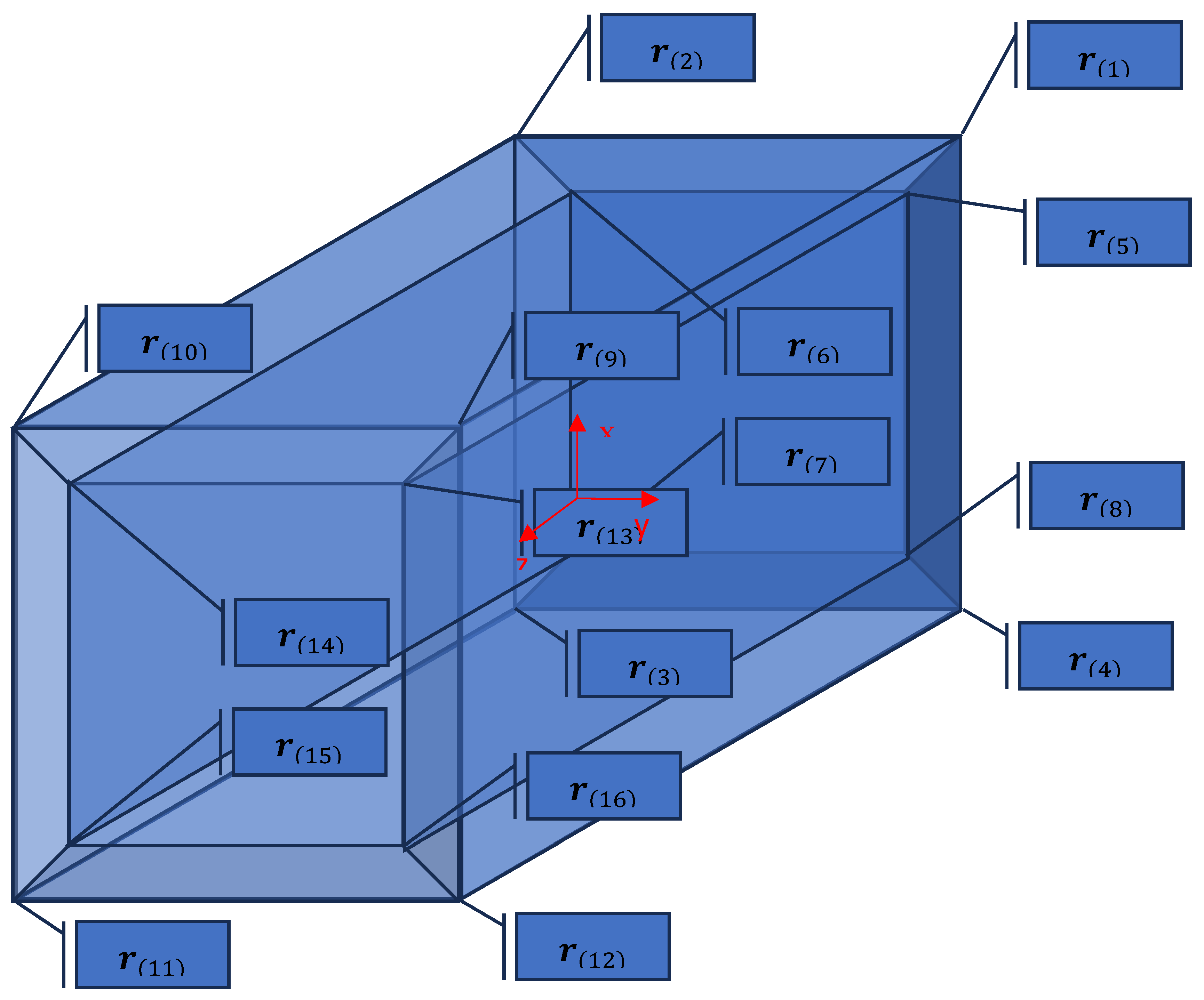
4.1. 4D Tesseract

The tesseract is a transfer of the classic cube concept to four dimensions. It is also referred to as a four-dimensional hypercube. The tesseract relates to the cube like the cube relates to the square. It has 16 corners, 32 edges of equal length, 24 square faces and is bounded by 8 cube-shaped cells. The radius-vectors of the vertices of the four-dimensional cuboid are:

${\mathit{r}}_{\left(\nu \right)}=‖\begin{array}{cc}\begin{array}{cc}a·{\left(-1\right)}^{Ceil\left({\displaystyle \frac{\nu }{8}}\right)},& b·{\left(-1\right)}^{Ceil\left({\displaystyle \frac{\nu }{4}}\right)},\end{array}& \begin{array}{cc}c·{\left(-1\right)}^{Ceil\left({\displaystyle \frac{\nu }{2}}\right)},& a·{\left(-1\right)}^{\nu }\end{array}\end{array}‖,\nu =1,\dots 16$.

In Eq. (69), the symbol $Ceil\left(\nu \right)$ signifies smallest integer greater than or equal to a real number $\nu$. The unit masses are applied on the vertex of the cuboid.

Figure 1. The cross-section x-y-z of the tesseract by one 3D-space. The unit masses are placed on the vertices of the rigid massless tesseract.

Figure 1. The cross-section x-y-z of the tesseract by one 3D-space. The unit masses are placed on the vertices of the rigid massless tesseract.

Specifically, for$N=4$, the non-zero components of the inertia tensor (22) are equal to:

$\begin{array}{c}\begin{array}{c}{I}^{1212}=-I^{2112}=-I^{1221}=I^{2121}=4\left(a^2+b^2\right),\\ I^{1313}=-I^{3113}=-I^{1331}=I^{3131}=4\left(a^2+c^2\right)\\ I^{1414}=-I^{4114}=-I^{1441}=I^{4114}=4\left(a^2+d^2\right),\end{array},\\ \begin{array}{c}{I}^{3232}=-I^{3223}=-I^{2332}=I^{2323}=4\left(b^2+c^2\right),\\ I^{2424}=-I^{4224}=-I^{2442}=I^{4242}=-4\left(b^2+d^2\right),\\ I^{3434}=-I^{3443}=-I^{4334}=I^{4343}=4\left(c^2+d^2\right).\end{array}\end{array}$The contacted form of the inertia tensor reads as:

$\mathbb{I}=32⟦\begin{array}{cc}\begin{array}{cc}{b}^2+c^2+d^2& \\ & a^2+c^2+d^2\end{array}& 0\\ 0& \begin{array}{cc}{a}^2+b^2+c^2& \\ & a^2+b^2+c^2\end{array}\end{array}⟧$,

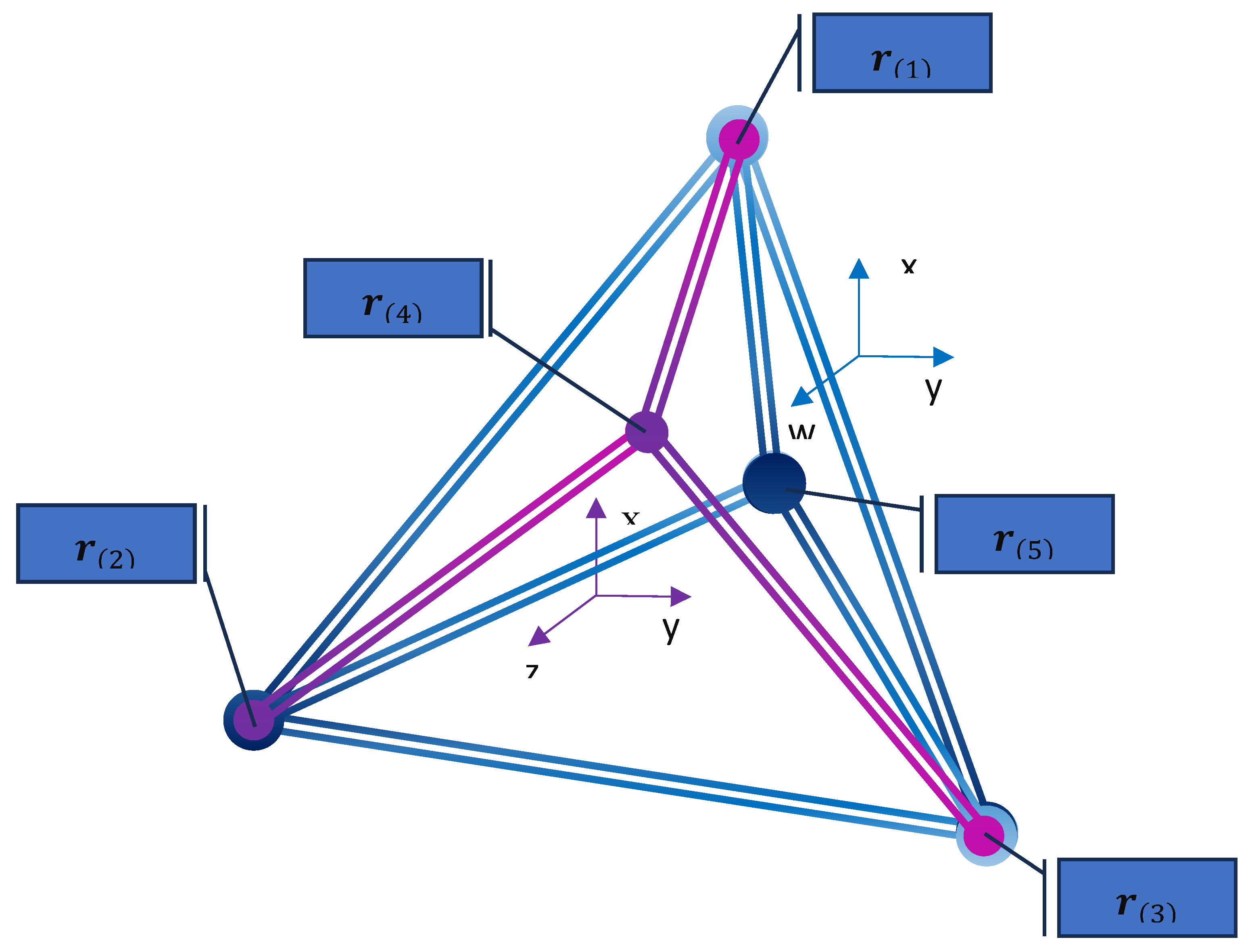
$\mu =32,{\mathbb{L}}_I^2=b^2+c^2+d^2,{\mathbb{L}}_{II}^2=a^2+c^2+d^2,{\mathbb{L}}_{III}^2=a^2+b^2+d^2,{\mathbb{L}}_{IV}^2=a^2+b^2+c^2.$4.2. 5D-Pentachoron

A pentachoron, also referred to as a 5-cell, pentatope, or four-dimensional hypertetrahedron, is a four-dimensional hyperpyramid with a tetrahedron. Its "base", or a 4-simplex, the simplest four-dimensional figure, polychoron. It consists of five tetrahedron-shaped cells and is the analog of the triangle (2-simplex) and the tetrahedron (3-simplex). The coordinates of the edges in 4D space are:

Figure 2. Two 3D projections of a 5-cell (xyz and xyw). The unit masses are placed on the vertices of the rigid massless pentachoron.

Figure 2. Two 3D projections of a 5-cell (xyz and xyw). The unit masses are placed on the vertices of the rigid massless pentachoron.

$R=⟦\begin{array}{c}\begin{array}{cc}\begin{array}{cc}a\sqrt{5}/4& b\sqrt{5}/4\\ a\sqrt{5}/4& -b\sqrt{5}/4\end{array}& \begin{array}{cc}c\sqrt{5}/4& -d/4\\ -c\sqrt{5}/4& -d/4\end{array}\\ \begin{array}{cc}-a\sqrt{5}/4& b\sqrt{5}/4\\ -a\sqrt{5}/4& -b\sqrt{5}/4\end{array}& \begin{array}{cc}-c\sqrt{5}/4& -d/4\\ c\sqrt{5}/4& -d/4\end{array}\end{array}\\ \begin{array}{cc}\begin{array}{cc} 0 & 0 \end{array}& \begin{array}{cc} 0 & d\end{array}\end{array}\end{array}⟧$

The masses on each vertex are equal to one. The non-zero components of the inertia tensor (22) are equal to:

$\begin{array}{c}\begin{array}{c}{I}^{1212}={\displaystyle \frac{5}{8}}\left(a^2+b^2\right),\\ I^{1313}={\displaystyle \frac{5}{8}}\left(a^2+c^2\right),\\ I^{1414}={\displaystyle \frac{5}{8}}\left(a^2+d^2\right),\end{array}\\ \begin{array}{c}{I}^{2424}={\displaystyle \frac{5}{8}}\left(b^2+d^2\right),\\ I^{3434}={\displaystyle \frac{5}{8}}\left(c^2+d^2\right),\\ I^{4141}={\displaystyle \frac{5}{8}}\left(a^2+d^2\right).\end{array}\end{array}$The inertia tensor is given by the matrix:

$\mathbb{I}=5⟦\begin{array}{cc}\begin{array}{cc}{b}^2+c^2+d^2& \\ & a^2+c^2+d^2\end{array}& 0\\ 0& \begin{array}{cc}{a}^2+b^2+d^2& \\ & a^2+b^2+c^2\end{array}\end{array}⟧$.

$\mu =5,{\mathbb{L}}_I^2=b^2+c^2+d^2,{\mathbb{L}}_{II}^2=a^2+c^2+d^2,{\mathbb{L}}_{III}^2=a^2+b^2+d^2,{\mathbb{L}}_{IV}^2=a^2+b^2+c^2.$Remarks. Consider the point mass rigid bodies with the equal masses in each vertex. Should the distances from each vertex to the center of mass prove equal for all vertices, then the inertia factor will be equal to the constant value, denoted as $\mathsf{\Theta }$, equal to one. It is important to note that the inertia factor remains constant under affine transformations, regardless of the shape of the bodies undergoing these transformations.

5. Inertia Tensor of a Rectangular Cuboid

The components of the components of the inertia tensor (22) of a cuboid (hyper-paralepidid) in multidimensional Euclidean space could be determined analogously. It is hypothesized that the material possesses homogeneity and an isotropic structure, characterized by an inherent constant unit density.

5.1. 4D Cuboid

In the context of $N=4$, this object can be regarded as a 4D analog of a conventional 3D parallelepiped. The geometric figure under consideration is rectangular in shape with parallel sides of different lengths $2a,2b,2c,2d$. It can be demonstrated that the hypervolume of the 4D analogue of a parallelepiped is equal to:

$V_{\left(4\right)}=2^4·a b c d$.

The non-zero components of the components of the inertia tensor (22) of the cuboid made of homogeneous material of the unit density are as follows:

$\begin{array}{c}\begin{array}{c}{I}^{1212}=-I^{2112}=-I^{1221}=I^{2121}={\displaystyle \frac{V_{\left(4\right)}}{3}}·\left(a^2+b^2\right),\\ I^{1313}=-I^{3113}=-I^{1331}=I^{3131}={\displaystyle \frac{V_{\left(4\right)}}{3}}·\left(a^2+c^2\right)\\ I^{1414}=-I^{4114}=-I^{1441}=I^{4114}={\displaystyle \frac{V_{\left(4\right)}}{3}}·\left(a^2+d^2\right),\end{array},\\ \begin{array}{c}{I}^{3232}=-I^{3223}=-I^{2332}=I^{2323}={\displaystyle \frac{V_{\left(4\right)}}{3}}·\left(b^2+c^2\right),\\ I^{2424}=-I^{4224}=-I^{2442}=I^{4242}={\displaystyle \frac{V_{\left(4\right)}}{3}}·\left(b^2+d^2\right),\\ I^{3434}=-I^{3443}=-I^{4334}=I^{4343}={\displaystyle \frac{V_{\left(4\right)}}{3}}·\left(c^2+d^2\right).\end{array}\end{array}$$\mathbb{I}={\displaystyle \frac{ V_{\left(4\right)}}{3}}·⟦\begin{array}{cc}\begin{array}{cc}{b}^2+c^2+d^2& \\ & a^2+c^2+d^2\end{array}& 0\\ 0& \begin{array}{cc}{a}^2+b^2+d^2& \\ & a^2+b^2+c^2\end{array}\end{array}⟧$.

$\mu =V_{\left(4\right)},{\mathbb{L}}_I^2={\displaystyle \frac{b^2+c^2+d^2}{3}},{\mathbb{L}}_{II}^2={\displaystyle \frac{a^2+c^2+d^2}{3}},{\mathbb{L}}_{III}^2={\displaystyle \frac{a^2+b^2+d^2}{3}},{\mathbb{L}}_{IV}^2={\displaystyle \frac{a^2+b^2+c^2}{3}}.$Particularly, a homogeneous hypercube has a constant unit density and all equal edge lengths $2a=2b=2\mathrm{c}=2d$.

5.2. 5D Cuboid

In the context of $N = 5$, the object can be regarded as a five-dimensional analog of a conventional three-dimensional parallelepiped. Its volume is equal to

$V_{\left(5\right)}=2^5·a b c d e$.

The non-zero components of the components of the inertia tensor (22) of 5D hyper-paralepidid are:

$\begin{array}{cc}\begin{array}{c}{I}^{1212}={\displaystyle \frac{V_{\left(5\right)}}{3}}·\left(a^2+b^2\right),\\ I^{1414}={\displaystyle \frac{V_{\left(5\right)}}{3}}·\left(a^2+d^2\right),\\ \begin{array}{c}{I}^{2323}={\displaystyle \frac{V_{\left(5\right)}}{3}}·\left(b^2+c^2\right),\\ I^{2525}={\displaystyle \frac{V_{\left(5\right)}}{3}}·\left(b^2+e^2\right),\\ I^{3535}={\displaystyle \frac{V_{\left(5\right)}}{3}}·\left(c^2+e^2\right),\end{array}\end{array}& \begin{array}{c}{I}^{1313}={\displaystyle \frac{V_{\left(5\right)}}{3}}·\left({-a}^2-c^2\right),\\ I^{1515}={\displaystyle \frac{V_{\left(5\right)}}{3}}·\left(a^2+e^2\right),\\ \begin{array}{c}{I}^{2424}={\displaystyle \frac{V_{\left(5\right)}}{3}}·\left({-b}^2-d^2\right),\\ I^{3434}={\displaystyle \frac{V_{\left(5\right)}}{3}}·\left(c^2+d^2\right),\\ I^{4545}={\displaystyle \frac{V_{\left(5\right)}}{3}}·\left(d^2+e^2\right).\end{array}\end{array}\end{array}$

6. Inertia Moments of Hyperspheres and Ellipsoids

6.1. 3D Ellipsoid

The initial step involves the calculation of volume and moments of inertia for a standard three-dimensional ellipsoid that represents a homogeneous unit density. The direct integration was conducted in order to determine the volume and the components of inertia tensor (22) in three-dimensional space $N = 3$:

$V_{\left(3\right)}=\underset{-a}{\overset{a}{\int }}\left\{{\int }_{-b\sqrt{1-{\left({\displaystyle \frac{x}{a}}\right)}^2}}^{b\sqrt{1-{\left({\displaystyle \frac{x}{a}}\right)}^2}}\left[{\int }_{-c\sqrt{1-{\left({\displaystyle \frac{x}{a}}\right)}^2{-\left({\displaystyle \frac{y}{a}}\right)}^2}}^{c\sqrt{1-{\left({\displaystyle \frac{x}{a}}\right)}^2{-\left({\displaystyle \frac{y}{a}}\right)}^2}}dz\right]dy\right\}dx={\displaystyle \frac{4\pi }{3}}abc$,

$I^{.1.1}=\left\{\underset{-a}{\overset{a}{\int }}\left\{{\int }_{-b\sqrt{1-{\left({\displaystyle \frac{x}{a}}\right)}^2}}^{b\sqrt{1-{\left({\displaystyle \frac{x}{a}}\right)}^2}}\left[{\int }_{-c\sqrt{1-{\left({\displaystyle \frac{x}{a}}\right)}^2{-\left({\displaystyle \frac{y}{a}}\right)}^2}}^{c\sqrt{1-{\left({\displaystyle \frac{x}{a}}\right)}^2{-\left({\displaystyle \frac{y}{a}}\right)}^2}}dz\right]dy\right\}{\mathrm{x}}^{2}dx\right\}={\displaystyle \frac{4\pi }{15}}{a}^{3}bc$,

$I^{.2.2}=\left\{\underset{-a}{\overset{a}{\int }}\left\{{\int }_{-b\sqrt{1-{\left({\displaystyle \frac{x}{a}}\right)}^2}}^{b\sqrt{1-{\left({\displaystyle \frac{x}{a}}\right)}^2}}\left[{\int }_{-c\sqrt{1-{\left({\displaystyle \frac{x}{a}}\right)}^2{-\left({\displaystyle \frac{y}{a}}\right)}^2}}^{c\sqrt{1-{\left({\displaystyle \frac{x}{a}}\right)}^2{-\left({\displaystyle \frac{y}{a}}\right)}^2}}dz\right]{\mathrm{y}}^{2}dy\right\}dx\right\}={\displaystyle \frac{4\pi }{15}}{b}^{3}ac,$$I^{.3.3}=\left\{\underset{-a}{\overset{a}{\int }}\left\{{\int }_{-b\sqrt{1-{\left({\displaystyle \frac{x}{a}}\right)}^2}}^{b\sqrt{1-{\left({\displaystyle \frac{x}{a}}\right)}^2}}\left[{\int }_{-c\sqrt{1-{\left({\displaystyle \frac{x}{a}}\right)}^2{-\left({\displaystyle \frac{y}{a}}\right)}^2}}^{c\sqrt{1-{\left({\displaystyle \frac{x}{a}}\right)}^2{-\left({\displaystyle \frac{y}{a}}\right)}^2}}{\mathrm{z}}^{2}dz\right]dy\right\}dx\right\}={\displaystyle \frac{4\pi }{15}}{c}^{3}ab$.

From Eq. (84),(85),(86) follow the common expression for the inertia tensor of second rank, §3.5, (Woan, 2000):

$\mathbb{I}={\displaystyle \frac{4\pi }{15}}abc·⟦\begin{array}{ccc}{b}^2+c^2& 0& 0\\ 0& a^2+c^2& 0\\ 0& 0& a^2+b^2\end{array}⟧={\displaystyle \frac{ V_{\left(3\right)}}{5}}⟦\begin{array}{ccc}{b}^2+c^2& 0& 0\\ 0& a^2+c^2& 0\\ 0& 0& a^2+b^2\end{array}⟧$.

$\mu =V_{\left(3\right)},{\mathbb{L}}_I^2={\displaystyle \frac{b^2+c^2}{5}},{\mathbb{L}}_{II}^2={\displaystyle \frac{a^2+c^2}{5}},{\mathbb{L}}_{III}^2={\displaystyle \frac{a^2+b^2}{5}}.$If $a=b=c=R$, the ellipsoid turns into the sphere with the following characteristics:

$\mu =V_{\left(3\right)}={\displaystyle \frac{4\pi }{3}}{R}^3$, ${\mathbb{L}}_{\alpha }^2={\displaystyle \frac{1}{5}}{R^2,\mathbb{I}}_{\alpha \alpha }={\displaystyle \frac{2}{5}}{R}^2\mu ,\alpha =I,II,III$.

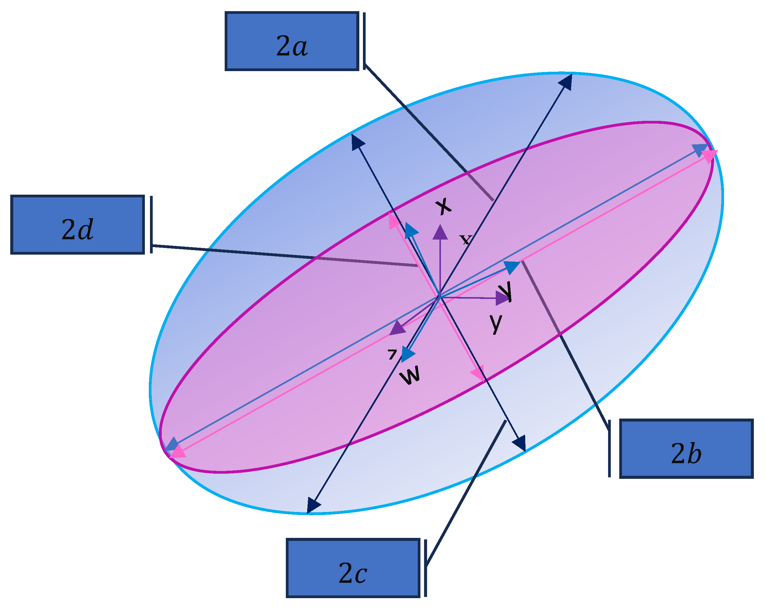
6.2. 4D Ellipsoid

In the context of $N=4$, the corresponding object can be regarded as a 4D analog of a conventional 3D ellipsoid. The computation of the volume and a component of inertia tensor (22) on 4D space leads to the integrals:

Figure 3. Two 3D projections of 4D ellipsoid.

Figure 3. Two 3D projections of 4D ellipsoid.

$V_{\left(4\right)}=\left\{\underset{-a}{\overset{a}{\int }}\left\{{\int }_{-b\sqrt{1-{\left({\displaystyle \frac{x}{a}}\right)}^2}}^{b\sqrt{1-{\left({\displaystyle \frac{x}{a}}\right)}^2}}\left[{\int }_{-c\sqrt{1-{\left({\displaystyle \frac{x}{a}}\right)}^2{-\left({\displaystyle \frac{y}{a}}\right)}^2}}^{c\sqrt{1-{\left({\displaystyle \frac{x}{a}}\right)}^2{-\left({\displaystyle \frac{y}{a}}\right)}^2}}\left\{\underset{-d\sqrt{1-{\left({\displaystyle \frac{x}{a}}\right)}^2{-\left({\displaystyle \frac{y}{a}}\right)}^2{-\left({\displaystyle \frac{z}{c}}\right)}^2}}{\overset{d\sqrt{1-{\left({\displaystyle \frac{x}{a}}\right)}^2{-\left({\displaystyle \frac{y}{a}}\right)}^2{-\left({\displaystyle \frac{z}{c}}\right)}^2}}{\int }}1 dw\right\}dz\right]dy\right\}dx\right\}={\displaystyle \frac{{\pi }^2}{2}}abcd$,

$I^{.1.1}=\left\{\underset{-a}{\overset{a}{\int }}\left\{{\int }_{-b\sqrt{1-{\left({\displaystyle \frac{x}{a}}\right)}^2}}^{b\sqrt{1-{\left({\displaystyle \frac{x}{a}}\right)}^2}}\left[{\int }_{-c\sqrt{1-{\left({\displaystyle \frac{x}{a}}\right)}^2{-\left({\displaystyle \frac{y}{a}}\right)}^2}}^{c\sqrt{1-{\left({\displaystyle \frac{x}{a}}\right)}^2{-\left({\displaystyle \frac{y}{a}}\right)}^2}}\left\{\underset{-d\sqrt{1-{\left({\displaystyle \frac{x}{a}}\right)}^2{-\left({\displaystyle \frac{y}{a}}\right)}^2{-\left({\displaystyle \frac{z}{c}}\right)}^2}}{\overset{d\sqrt{1-{\left({\displaystyle \frac{x}{a}}\right)}^2{-\left({\displaystyle \frac{y}{a}}\right)}^2{-\left({\displaystyle \frac{z}{c}}\right)}^2}}{\int }} dw\right\}dz\right]dy\right\}{\mathrm{x}}^{2}dx\right\}={\displaystyle \frac{{\pi }^2}{12}}{a}^{3}bcd$,

$I^{.2.2}=\left\{\underset{-a}{\overset{a}{\int }}\left\{{\int }_{-b\sqrt{1-{\left({\displaystyle \frac{x}{a}}\right)}^2}}^{b\sqrt{1-{\left({\displaystyle \frac{x}{a}}\right)}^2}}\left[{\int }_{-c\sqrt{1-{\left({\displaystyle \frac{x}{a}}\right)}^2{-\left({\displaystyle \frac{y}{a}}\right)}^2}}^{c\sqrt{1-{\left({\displaystyle \frac{x}{a}}\right)}^2{-\left({\displaystyle \frac{y}{a}}\right)}^2}}\left\{\underset{-d\sqrt{1-{\left({\displaystyle \frac{x}{a}}\right)}^2{-\left({\displaystyle \frac{y}{a}}\right)}^2{-\left({\displaystyle \frac{z}{c}}\right)}^2}}{\overset{d\sqrt{1-{\left({\displaystyle \frac{x}{a}}\right)}^2{-\left({\displaystyle \frac{y}{a}}\right)}^2{-\left({\displaystyle \frac{z}{c}}\right)}^2}}{\int }} dw\right\} dz \right]y^{2}dy\right\}dx\right\}={\displaystyle \frac{{\pi }^2}{12}}{b}^{3}acd$,

$I^{.3.3}=\left\{\underset{-a}{\overset{a}{\int }}\left\{{\int }_{-b\sqrt{1-{\left({\displaystyle \frac{x}{a}}\right)}^2}}^{b\sqrt{1-{\left({\displaystyle \frac{x}{a}}\right)}^2}}\left[{\int }_{-c\sqrt{1-{\left({\displaystyle \frac{x}{a}}\right)}^2{-\left({\displaystyle \frac{y}{a}}\right)}^2}}^{c\sqrt{1-{\left({\displaystyle \frac{x}{a}}\right)}^2{-\left({\displaystyle \frac{y}{a}}\right)}^2}}\left\{\underset{-d\sqrt{1-{\left({\displaystyle \frac{x}{a}}\right)}^2{-\left({\displaystyle \frac{y}{a}}\right)}^2{-\left({\displaystyle \frac{z}{c}}\right)}^2}}{\overset{d\sqrt{1-{\left({\displaystyle \frac{x}{a}}\right)}^2{-\left({\displaystyle \frac{y}{a}}\right)}^2{-\left({\displaystyle \frac{z}{c}}\right)}^2}}{\int }} dw\right\}{\mathrm{z}}^{2}dz\right]dy\right\}dx\right\}={\displaystyle \frac{{\pi }^2}{12}}{c}^{3}acd$,

$I^{.4.4}=\left\{\underset{-a}{\overset{a}{\int }}\left\{{\int }_{-b\sqrt{1-{\left({\displaystyle \frac{x}{a}}\right)}^2}}^{b\sqrt{1-{\left({\displaystyle \frac{x}{a}}\right)}^2}}\left[{\int }_{-c\sqrt{1-{\left({\displaystyle \frac{x}{a}}\right)}^2{-\left({\displaystyle \frac{y}{a}}\right)}^2}}^{c\sqrt{1-{\left({\displaystyle \frac{x}{a}}\right)}^2{-\left({\displaystyle \frac{y}{a}}\right)}^2}}\left\{\underset{-d\sqrt{1-{\left({\displaystyle \frac{x}{a}}\right)}^2{-\left({\displaystyle \frac{y}{a}}\right)}^2{-\left({\displaystyle \frac{z}{c}}\right)}^2}}{\overset{d\sqrt{1-{\left({\displaystyle \frac{x}{a}}\right)}^2{-\left({\displaystyle \frac{y}{a}}\right)}^2{-\left({\displaystyle \frac{z}{c}}\right)}^2}}{\int }}{\mathrm{w}}^{2}dw\right\}dz\right]dy\right\}dx\right\}={\displaystyle \frac{{\pi }^2}{12}}{d}^{3}abc$.

The contracted tensor notation (24) of the moment of inertia of a homogeneous ellipsoid with density $\rho =1$ reads:

$\mathbb{I}={\displaystyle \frac{{\pi }^2}{2}}abcd·⟦\begin{array}{cc}\begin{array}{cc}{\displaystyle \frac{b^2+c^2+d^2}{6}}& \\ & {\displaystyle \frac{a^2+c^2+d^2}{6}}\end{array}& 0\\ 0& \begin{array}{cc}{\displaystyle \frac{a^2+b^2+d^2}{6}}& \\ & {\displaystyle \frac{a^2+b^2+c^2}{6}}\end{array}\end{array}⟧$,

$\mathbb{I}={\displaystyle \frac{V_{\left(4\right)}}{6}}·⟦\begin{array}{cc}\begin{array}{cc}{b}^2+c^2+d^2& \\ & a^2+c^2+d^2\end{array}& 0\\ 0& \begin{array}{cc}{a}^2+b^2+d^2& \\ & a^2+b^2+c^2\end{array}\end{array}⟧$,

$\mu =V_{\left(4\right)},{\mathbb{L}}_I^2={\displaystyle \frac{b^2+c^2+d^2}{6}},{\mathbb{L}}_{II}^2={\displaystyle \frac{a^2+c^2+d^2}{6}},{\mathbb{L}}_{III}^2={\displaystyle \frac{a^2+b^2+d^2}{6}}, {\mathbb{L}}_{IV}^2={\displaystyle \frac{a^2+b^2+c^2}{6}}$.

If all half-axes are of equal length, $a=b=c=d=R$. In this case the 4D-ellipsoid turns into 4D-sphere with the following characteristics:

$\mu =V_{\left(4\right)}={\displaystyle \frac{{\pi }^2}{2}}{R}^4$, ${\mathbb{L}}_{\alpha }^2={\displaystyle \frac{1}{2}}{R^2,\mathbb{I}}_{\alpha \alpha }={\displaystyle \frac{\mu }{2}}{R}^2$, $\alpha =I,II,III,IV$.

The 5D-ellipsoid may be studied using an analogous approach.

6.3. Hyperspheres

For all hyperspheres of arbitrary dimensions, the half-axes of Poinsot's inertia ellipsoids are equal. The Poinsot's ellipsoids turns into the hyperspheres in the same dimension, by with the gyration radius ${\mathbb{L}}_{\alpha }^2,\alpha =1,..,N$, which depends unto the dimension of space $N$. The evaluation of the gyration radius is based on the outcomes reported in extant literature (Huber, 1982), (Salgia, 1983), (Hong & Hong, 2014), (Bender & Mead, 1995).

The volume $V_{\left(N\right)}$and the surface ${\partial V}_{\left(N\right)}$of the sphere in the space of dimension $N$ were defined in (Huber, 1982):

$V_{\left(N\right)}={\displaystyle \frac{{\pi }^{\mathrm{N}/2}}{\mathsf{\Gamma }\left(1+\frac{N}{2}\right)}}{R}^N$, ${\partial V}_{\left(N\right)}={\displaystyle \frac{{\pi }^{\mathrm{N}/2}}{\mathsf{\Gamma }\left(1+\frac{N}{2}\right)}}N{R}^{N-1}$.

The aforementioned method (Bender & Mead, 1995) is applied for the hypersphere of the radius $R.$In order to perform the necessary calculations of mass moments of inertia, it is first necessary to determine the moment of weight $p$ about the polar axis, which is normal to the space of the sphere. This auxiliary value is equal to:

$I_{(N,p)}^P={\int }_0^R{\partial V}_{\left(N\right)}{R}^{p}dR={\displaystyle \frac{{\pi }^{N/2}}{\mathsf{\Gamma }\left(\frac{N}{2}+1\right)}}{\displaystyle \frac{N}{N+p}}{R}^{N+p}$.

Particularly, for $p=2$ the inertia moments of the second order of the homogeneous hyperspheres with the density $\rho =1$ are:

$I_{(N,2)}^P={\displaystyle \frac{N{\pi }^{N/2}}{\mathsf{\Gamma }\left(\frac{N}{2}+1\right)}}{\displaystyle \frac{R^{N+2}}{N+2}}.$The combination of equations (101) and (99) yields for the polar moments of inertia:

$\begin{array}{cc}{\displaystyle \frac{I_{(N,2)}^P}{V_{\left(N\right)}}}={\displaystyle \frac{N }{N+2}}{R}^2.& \end{array}.$It has been established that the value of the inertia factor is equivalent to the constant value (102) for hyperspheres in spaces of dimension $N$. Since the inertia factor remains constant under affine transformations, the same value of the inertia factor is obtained for ellipsoids in spaces of the same dimension.

The moment of second order about a diameter $I_{(N,2)}^D\equiv {\mathbb{I}}_{\alpha \alpha }, \alpha =I,\dots ,N$ was defined in (Bender & Mead, 1995). For the calculation the following integral will be used, Eq. 3.621, (Gradshteyn, Ryzhik, Geronimus, Tseytlin, & Jeffrey, 2014):

$\mathsf{\phi }\left(\mu \right)\stackrel{\scriptscriptstyle\mathrm{def}}{=}{\int }_0^{{\displaystyle \frac{\pi }{2}}}{\mathrm{s}\mathrm{i}\mathrm{n}}^{\mu }x dx={\int }_0^{{\displaystyle \frac{\pi }{2}}}{\mathrm{c}\mathrm{o}\mathrm{s}}^{\mu }x dx={\displaystyle \frac{\sqrt{\pi }}{2}} {\displaystyle \frac{\mathsf{\Gamma }\left(\frac{\mu +1}{2}\right)}{\mathsf{\Gamma }\left(\frac{\mu }{2}+1\right)}}$.

The moment of weight $p$ about a diameter equal to:

$I_{\left(N,p\right)}^D=\mathsf{\Phi }\left(N,p\right)I_{(N,p)}^P={\displaystyle \frac{{\pi }^{N/2}}{\mathsf{\Gamma }\left(\frac{N-1}{2}\right)}}{\displaystyle \frac{\mathsf{\Gamma }\left(\frac{N+p-1}{2}\right)}{\mathsf{\Gamma }\left(\frac{N+p+1}{2}\right)}}{R}^{N+p}$.

The auxiliary function $\mathsf{\Phi }\left(N,p\right)$ is defined in Eq. (104) with the special function (105):

$\mathsf{\Phi }\left(N,p\right)\stackrel{\scriptscriptstyle\mathrm{def}}{=}{\displaystyle \frac{\mathsf{\phi }\left(N+p-2\right)}{\mathsf{\phi }\left(N-2\right)}}$.

The combination of equations (104) and (99) yields for the polar moments of inertia${\mathbb{I}}_{\alpha \alpha }$ and the gyration radii ${\mathbb{L}}_{\alpha }$ of the hyperspheres in the space of dimension $N$ :

$\begin{array}{cc}{\displaystyle \frac{I_{(N,2)}^D}{V_{\left(N\right)}}}={\displaystyle \frac{N-1 }{N+2}}{R}^2,& {\mathbb{L}}_{\alpha }^2={\displaystyle \frac{N-1 }{N+2}}{R^2,\mathbb{I}}_{\alpha \alpha }={\displaystyle \frac{N-1 }{N+2}}{\mu R}^2\end{array}, \alpha =I,\dots ,N.$The result of equation (106) is equivalent to the values obtained from equations (89) and (98) in the cases $N = 3$ and $N = 4$, respectively. The results obtained from equation (106) facilitate the calculation of the diagonal moments of inertia, which bear a resemblance to the structures depicted in equations (87) and (96).

7. Solutions of the Euler Equations in 4D Spaces

7.1. All Moments of Inertia Equal

The system of nonlinear ordinary differential Eq. (52) is nonlinear and depend upon six initial conditions and six fixed components of inertia tensor. The coefficients of equations (52) depend upon four parameters $a,b,c,d$ or ${\mathbb{L}}_{\alpha }^2,\alpha =1,..,4$.

In some special cases the system (52) allows the closed form solutions. In the initial phase of this investigation, we shall establish the solution to the Euler equations (52) in the case of an equal moment of inertia across all possible axes of rotation:

$a=b=c=d.$The Platonic bodies and hyperspheres satisfy this condition, as we can see form Eq.(89),(98). For such bodies all gyration radii are equal. In this case the second term in all left sides of the equations (52) vanish. The time derivatives of the rotation components nullify in the absence of the external moments:

${\displaystyle \frac{d{\omega }_{12}}{dt}}={\displaystyle \frac{d{\omega }_{23}}{dt}}={\displaystyle \frac{d{\omega }_{13}}{dt}}={\displaystyle \frac{d{\omega }_{24}}{dt}}={\displaystyle \frac{d{\omega }_{14}}{dt}}={\displaystyle \frac{d{\omega }_{34}}{dt}}=0$.

Consequently, it is evident that all components of the rotation velocity are sustained over a given period of time. It can be posited that this behavior holds in all multidimensional Euclidean spaces.

7.2. A Sole Different and One Triad of Equal Moments of Inertia

The second case corresponds to three equal principal moments of inertia with one distinct principal moment. In the absence of any restrictions, the equal principal moments of inertia are set to one, and the distinct one is referred to as $\kappa$:

$a=b=c=1, d=\kappa$.

The aforementioned equations (53)..(58) can be simplified to three nullifying expressions and three linear ordinary differential equations with constant coefficients:

${\displaystyle \frac{d{\omega }_{12}}{dt}}=0,$${\omega }_{12}\left(t=0\right)=c_3$,

${\displaystyle \frac{d{\omega }_{23}}{dt}}=0$, ${\omega }_{23}\left(t=0\right)=c_1$,

${\displaystyle \frac{d{\omega }_{13}}{dt}}=0$, ${\omega }_{13}\left(t=0\right)=c_2$.

The resolution (110)…(112)of three ordinary differential equations of a nullifying nature guarantees that the three rotation velocities remain constant. It is evident that the coefficients of three additional ordinary differential equations are contingent upon the initial three constant velocities ${{\omega }_{23}\equiv c}_1,{\omega }_{13}\equiv c_2,{\omega }_{12}\equiv c_3$:

$\left(1+{\kappa }^2\right){\displaystyle \frac{d{\omega }_{24}}{dt}}+\left({1-\kappa }^2\right)\left(c_3{\omega }_{14}-c_1{\omega }_{34}\right)=0$,

$\left(1+{\kappa }^2\right){\displaystyle \frac{d{\omega }_{14}}{dt}}-\left({1-\kappa }^2\right)\left(c_3{\omega }_{24}+c_2{\omega }_{34}\right)=0$,

$\left(1+{\kappa }^2\right){\displaystyle \frac{d{\omega }_{34}}{dt}}+\left({1-\kappa }^2\right)\left(c_2{\omega }_{14}+c_1{\omega }_{24}\right)=0$.

The equations (113)…(115) are the linear ordinary differential equations of the first order with the constant coefficients. The closed form solution of the Eq. (113)…(115) reads:

${\omega }_{14}\left(t\right)=c_6\mathbb{C}+c_5\mathbb{S}+c_4$,

${\omega }_{24}={\displaystyle \frac{{{c_{1}c}_{2}c}_6-c_3{c}_5\sqrt{{c_1}^2+{c_2}^2+{c_3}^2}}{{c_2}^2+{c_3}^2}}·\mathbb{C}+{\displaystyle \frac{{{c_{1}c}_{2}c}_5+c_3{c}_6\sqrt{{c_1}^2+{c_2}^2+{c_3}^2}}{{c_2}^2+{c_3}^2}}·\mathbb{S}-{\displaystyle \frac{c_2{c}_4}{c_1}}$,

${\omega }_{34}=-{\displaystyle \frac{{{{c_1}^{2}c}_{3}c}_6+c_1{c}_2{c}_5\sqrt{{c_1}^2+{c_2}^2+{c_3}^2}}{c_1\left({c_2}^2+{c_3}^2\right)}}·\mathbb{C}+{\displaystyle \frac{-{{{c_1}^{2}c}_{3}c}_5+c_1{c}_2{c}_6\sqrt{{c_1}^2+{c_2}^2+{c_3}^2}}{c_1\left({c_2}^2+{c_3}^2\right)}}·\mathbb{S}+{\displaystyle \frac{c_3{c}_4}{c_1}}$.

The auxiliary functions in Eqs. (116)…(118) are the following:

$\mathbb{C}\left(t\right)\stackrel{\scriptscriptstyle\mathrm{def}}{=}\mathrm{c}\mathrm{o}\mathrm{s}\left({\displaystyle \frac{{\kappa }^2-1}{{\kappa }^2+1}}·t·\sqrt{{c_1}^2+{c_2}^2+{c_3}^2}\right)$,

$\mathbb{S}\left(t\right)\stackrel{\scriptscriptstyle\mathrm{def}}{=}\mathrm{s}\mathrm{i}\mathrm{n}\left({\displaystyle \frac{{\kappa }^2-1}{{\kappa }^2+1}}·t·\sqrt{{c_1}^2+{c_2}^2+{c_3}^2}\right)$.

The rotation velocities are harmonically oscillating functions. The oscillation periods of the third last velocities depend on the first three constant velocities $c_1,c_2,c_3$. The constants $c_4,c_5,c_6$ are contingent on the initial conditions that have been imposed upon the remaining three velocities.

7.3. Two Duets of Equal Moments of Inertia

The third closely solved case corresponds to two pairs of equal principal moments of inertia. The first two equal principal moments of inertia are set to one, and the second two are referred to as $\kappa$:

$a=b=1, d=c=\kappa$.

The aforementioned equations (53)..(58) can be simplified to two nullifying expressions and four linear ordinary differential equations with constant coefficients

${\displaystyle \frac{d{\omega }_{12}}{dt}}=0,$${\omega }_{12}\left(t=0\right)=c_1$,

${\displaystyle \frac{d{\omega }_{34}}{dt}}=0$, ${\omega }_{34}\left(t=0\right)=c_2$,

$\left(1+{\kappa }^2\right){\displaystyle \frac{d{\omega }_{13}}{dt}}+\left({\kappa }^2-1\right)\left(c_1{\omega }_{23}-c_2{\omega }_{14}\right)=0$,

$\left(1+{\kappa }^2\right){\displaystyle \frac{d{\omega }_{14}}{dt}}+\left({\kappa }^2-1\right)\left(c_2{\omega }_{13}+c_1{\omega }_{24}\right)=0$,

$\left(1+{\kappa }^2\right){\displaystyle \frac{d{\omega }_{34}}{dt}}-\left({\kappa }^2-1\right)\left(c_2{\omega }_{24}+c_1{\omega }_{13}\right)=0$,

$\left(1+{\kappa }^2\right){\displaystyle \frac{d{\omega }_{24}}{dt}}-\left({1-\kappa }^2\right)\left(c_1{\omega }_{14}-c_2{\omega }_{23}\right)=0$.

The equations are the linear ordinary differential equations of the first order. The closed form solution of the Eq. (124),(125),(126),(127) reads:

${\omega }_{13}=c_3 {·\mathbb{F}}_1+c_4 ·{\mathbb{F}}_2+c_5 ·{\mathbb{F}}_3+c_6 {·\mathbb{F}}_4$,

${\omega }_{14}=c_4· {\mathbb{F}}_1-c_3· {\mathbb{F}}_2-c_6· {\mathbb{F}}_3+c_5· {\mathbb{F}}_4$,

${\omega }_{23}=c_4· {\mathbb{F}}_1-c_3· {\mathbb{F}}_2+c_6 ·{\mathbb{F}}_3-c_5 ·{\mathbb{F}}_4$,

${\omega }_{24}=-c_3 ·{\mathbb{F}}_1-c_4· {\mathbb{F}}_2+c_5· {\mathbb{F}}_3+c_6 ·{\mathbb{F}}_4$.

There are the following auxiliary functions in Eqs. (128)..(131):

${\mathbb{F}}_1\left(t\right)=\mathrm{s}\mathrm{i}\mathrm{n}\left({\displaystyle \frac{{\kappa }^2-1}{{\kappa }^2+1}}\left(c_1-c_2\right)t\right)\equiv \mathrm{s}\mathrm{i}\mathrm{n}\left({\omega }_{1}t\right)$, ${\mathbb{F}}_2\left(t\right)=\mathrm{c}\mathrm{o}\mathrm{s}\left({\displaystyle \frac{{\kappa }^2-1}{{\kappa }^2+1}}\left(c_1-c_2\right)t\right)\equiv \mathrm{c}\mathrm{o}\mathrm{s}\left({\omega }_{1}t\right)$,

${\mathbb{F}}_3\left(t\right)=\mathrm{s}\mathrm{i}\mathrm{n}\left({\displaystyle \frac{{\kappa }^2-1}{{\kappa }^2+1}}\left(c_1+c_2\right)t\right)\equiv \mathrm{s}\mathrm{i}\mathrm{n}\left({\omega }_{2}t\right)$, ${\mathbb{F}}_4\left(t\right)=\mathrm{c}\mathrm{o}\mathrm{s}\left({\displaystyle \frac{{\kappa }^2-1}{{\kappa }^2+1}}\left(c_1+c_2\right)t\right)\equiv \mathrm{c}\mathrm{o}\mathrm{s}\left({\omega }_{2}t\right)$.

The rotation velocities (128)…(131) are shown once again to be harmonic oscillating functions. The oscillation frequencies of the four last velocities are determined by the first two constant velocities, $c_1,c_2$:

$\begin{array}{cc}{\omega }_1={\displaystyle \frac{{\kappa }^2-1}{{\kappa }^2+1}}·\left(c_1-c_2\right),& {\omega }_2={\displaystyle \frac{{\kappa }^2-1}{{\kappa }^2+1}}·\left(c_1+c_2\right)\end{array}$.

The remaining three velocities are constrained by initial conditions that are imposed upon them; these are denoted $c_3,c₄,c₅,c₆.$In general case of the different four parameters $a,b, d,c$ the Euler equations could be solved numerically. The solution to the differential equations (52) manifests as oscillating behavior in the rotational velocities, as observed over the given interval of time.

8. Conclusions and Directions for Future Research

The present manuscript undertakes a study of the rotational behavior of rigid bodies in spaces of higher dimensions. It is demonstrated that two integrals of motion exist for an unperturbed rotational motion. In the context of Euclidian spaces of dimension four, the number of rotational degrees of freedom is six. In the case of a five-dimensional Euclidian space, the number of rotational degrees of freedom is increased to ten. The Euler equations are derived using the tensor representation of rotational velocities. The closed form solutions were discovered for a certain relation between the principal moments of inertia.

Spin angular momentum, also known as spin, is a fundamental property of all particles, regardless of their status as elementary or composite entities. It is an intrinsic property, independent of spatial coordinates, and manifests as the particle's inherent angular momentum. The succeeding study will explore the quantization of the rotation motion of four-dimensional rigid bodies in order to analyze the symmetries and relations between the virtual moments of inertia in higher dimensions. These can be experimentally observed on the verifiable three-dimensional projections of the four- or five-dimensional hypothetical spaces on the microscopic scale.

References

- Bender, C., & Mead, L. (1995). D-dimensional moments of inertia. Am. J. Physics, Vol 63(11), 1011-1014.
- Cayley, A. (1846). Sur quelques propriétés des déterminants gauches. Journal für die reine und angewandte Mathematik, 32.
- Gradshteyn, I. S., Ryzhik, I. M., Geronimus, Y. V., Tseytlin, M. Y., & Jeffrey, A. (2014). Table of Integrals, Series, and Products. Amsterdam : Academic Press, Elsevier.
- Hestenes, D. (2002). New Foundations for Classical Mechanics. NEW YORK, BOSTON, DORDRECHT, LONDON, MOSCOW: KLUWER ACADEMIC PUBLISHERS.
- Hong, S.-I., & Hong, S.-C. (2014). Moments of inertia of spheres without integration in arbitrary dimensions. European Journal of Physics, 35, 025003. [CrossRef]
- Huber, G. (1982). The Gamma Function Derivation of n-Sphere Volumes. American Mathematical Monthly, 89(5), 301–302. [CrossRef]
- Krey, U., & Owen, A. (2007). Basic Theoretical Physics. A Concise Review. Berlin Heidelberg : Springer-Verlag.
- Landau, L., & Lifshitz, E. M. (1976). Mechanics: Volume 1, Course of Theoretical Physics. Oxford: Butterworth-Heinemann.
- Parker, E. (2024). The Ricci decomposition of the inertia tensor for a rigid body in arbitrary spatial dimensions. International Journal of Theoretical Physics. [CrossRef]
- Poinsot, L. (1834). Theorie Nouvelle de la Rotation des Corps. Paris: Bachelier.
- Salgia, R. (1983). VOLUME OF AN n-DIMENSIONAL UNIT SPHERE. Pi Mu Epsilon Journal, 496-501, https://www.jstor.org/stable/24337805.
- Ten Bosch, M. (2020). N-Dimensional Rigid Body Dynamics. ACM Trans. 39(4) Article 55. [CrossRef]
- Woan, G. (2000). The Cambridge Handbook of Physics Formulas. Cambridge: Cambridge University Press.