
Submitted:
31 July 2025
Posted:
01 August 2025
You are already at the latest version
Abstract
Rio Grande do Sul accounts for 22% of Brazil’s losses from extreme events, mainly droughts and floods. The state had the second-worst economic performance in the country between 2000 and 2022. This study quantifies the impacts of major events like droughts, floods, and the Covid-19 pandemic on economic sectors. Three methods were applied: structural breaks, recovery time, and sector-specific loss estimates. The analysis covers 15,365,123 observations of monthly invoice values from January 2017 to April 2025, involving 357,001 companies paying value-added tax on consumption. The results indicate that negative structural breaks have occurred in a few sectors, accounting for 5% of the state's economy. The recovery time followed a similar trajectory between droughts and Covid-19. The average recovery time for sectors was 12 months for Covid-19, while it was close to 6 months for other events. The sectors most impacted were travel, artistic activities, machinery and equipment industry, accommodation and domestic services. As for aggregated loss estimates, they were most relevant during the Covid-19 event, with -8%, followed by floods with -1%, and droughts with 0%. The results indicate remarkable overall economic resilience. Furthermore, sectors such as information technology, consulting, business services, and healthcare performed exceptionally well.
Keywords:
natural hazards and sustainability
; natural hazards assessment
; disaster risk management and sustainability
; post-disaster recovery
; economic resilience
; regional development planning and policy
1. Introduction
Rio Grande do Sul (RS), the southernmost state in Brazil, has been affected by extreme weather events such as droughts and floods, which have reoccurred again following the COVID-19 pandemic. Although the economy of RS is relatively diversified, agriculture and agribusiness continue to play a fundamental role in its overall production. However, between 2000 and 2024, RS recorded the second-lowest GDP growth rate among all Brazilian states. It is also the state with the highest economic losses caused by weather events, accounting for 22% of the total damage reported in both the public and private sectors nationwide. Following RS are Minas Gerais (MG) with 10%, Santa Catarina (SC) with 9%, and Paraná (PR) with 8% (Figure 1). The southern region of Brazil stands out as a hotspot for extreme events, representing 39% of the country’s total losses.
Figure 2 shows that the loss in RS from 2000 to 2024 is close to 140 billion reais, more than double that of the hard-hit states of Minas Gerais and Santa Catarina. In terms of the number of events, Minas Gerais reached 8,635, Rio Grande do Sul 8,369 and Santa Catarina 7,594. Bahia is the 4th state with the highest number of events with 4,952.
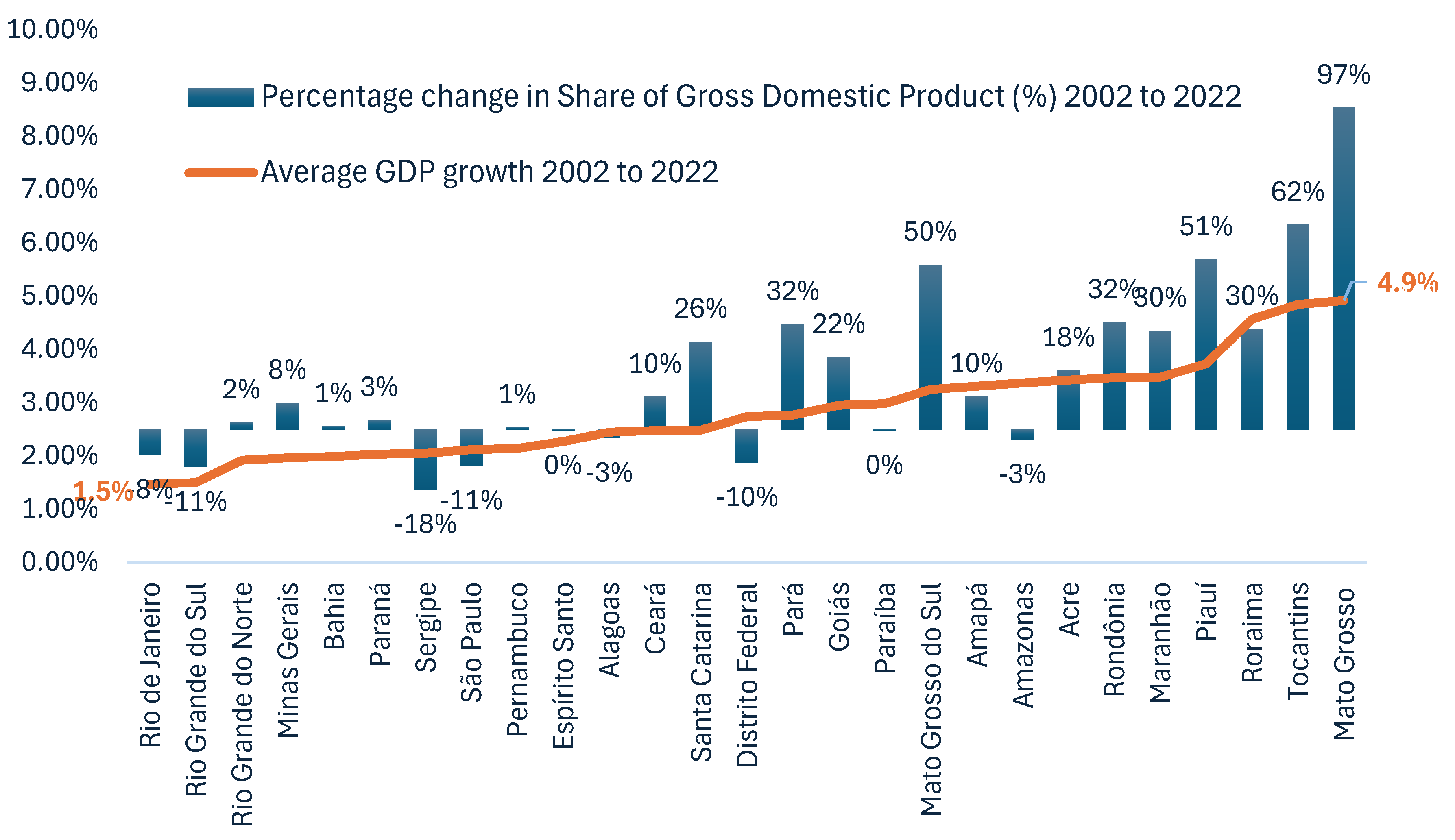
An analysis of the 2002–2022 period reveals that Rio Grande do Sul (RS) demonstrated relatively weak economic performance. RS recorded an average growth of just 1.50%, ranking only slightly ahead of Rio de Janeiro (RJ), which posted the lowest growth rate in the country at 1.47%. In contrast, Mato Grosso experienced an average growth of 4.9% during the same period, nearly doubling its share of the national GDP. Meanwhile, the states of Sergipe, São Paulo, Rio Grande do Sul, the Federal District, and Rio de Janeiro saw notable declines in their respective contributions to Brazil’s GDP.
Figure 3.
Average GDP growth of the States and share of the national product, from 2002 to 2022. Source: Prepared by the authors. IBGE – Instituto Brasileiro de Geografia e Estatística.
Figure 3.
Average GDP growth of the States and share of the national product, from 2002 to 2022. Source: Prepared by the authors. IBGE – Instituto Brasileiro de Geografia e Estatística.
Rio Grande do Sul is characterized by a strong presence in the primary sector, particularly in agriculture and livestock, and plays a significant role in Brazil’s export economy. Table 1 presents the main economic sectors in the state, measured by the value of invoices subject to the state’s consumption tax. The commerce sector ranks first, followed by food manufacturing. As of 2024, the state has approximately 165,000 companies, with around three-quarters classified as small businesses operating under a simplified tax regime. In terms of sectoral distribution, commerce stands out with nearly 100,000 companies. Notably, there is also substantial activity in vehicle and motorcycle-related commerce, followed by the food industry and the wholesale sector.
A recent study evaluates the impact of tax incentives in Rio Grande do Sul (RS) on company efficiency, specifically in terms of value-added generation and job creation. The findings indicate higher efficiency in the chemical and leather-footwear sectors, while the electronics, beverages, food, and agro-industrial sectors demonstrate lower efficiency. The results also underscore the importance of human capital as a determinant of efficiency, with the agro-industrial sector notably distinguished by its strong export orientation (Tonetto et al., 2025b).
Table 2 presents the total public and private losses in Rio Grande do Sul (RS) since 2000—adjusted for inflation—alongside the frequency of hydrometeorological events recorded at the municipal level. Droughts emerge as the most frequent and economically damaging phenomenon, although heavy rains and floods also occur with high regularity. RS continues to face significant exposure to a range of hydrometeorological hazards. According to the Governor’s 2024 message to the Legislative Assembly, droughts are the most common type of disaster in the state, followed by floods (Governo do Estado do Rio Grande do Sul, 2024). A study examining the duration of droughts in 2020, 2022, and 2023—based on the time required for economic recovery at the municipal level—found that, following each drought event, at least 75% of the affected municipalities recovered economically within three months, while 24% of municipalities were unaffected by any of these events (Tonetto et al., 2024).
It is important to note that according to the Inter-American Development Bank (IDB) and the World Bank, the total effects of floods in RS in 2024 were estimated at BRL 88.9 billion, using their own methodology, and this was the largest catastrophe in the history of RS. The flood directly affected 876,565 people, with 95 municipalities declaring a state of calamity and 323 declaring a state of emergency. A study showed that the municipalities of RS have limited fiscal response capacity for these events (Tonetto et al., 2025).
The objective of this study is to estimate the impacts of extreme events that occurred between 2020 and 2024 on the economic sectors of Rio Grande do Sul (RS) and to identify those sectors most susceptible to crises. The analysis includes estimates of both the magnitude of losses and the duration of the impacts. The methodology combines the Bai and Perron (1998) structural break model, Kaplan-Meier survival analysis adapted to measure recovery time, and sector-specific loss estimates across 74 economic sectors. The data employed consist of the total monthly invoice values issued by companies operating in the state, covering both B2C and B2B transactions. Each company is classified by sector according to the Brazilian Institute of Geography and Statistics (IBGE).
Following this introduction, Section 2 provides a review of the literature on the economic impacts of natural disasters. Section 3 describes the methodologies used, including descriptive statistics of the dataset and a detailed explanation of the procedures adopted. Section 4 presents and discusses the results, and finally, Section 5 summarizes the main conclusions of the study
2. Literature Review on Economic Impacts of Natural Disasters
The 2015 Paris Agreement has emerged as the most important scientific safeguard for climate action worldwide. The quest to limit the increase in global average temperature to 2°C above pre-industrial levels and pursue a reduction to 1.5°C will greatly reduce the effects of climate change (Kirchen and Pichler, 2025). A study on the effects of climate change, considering the non-linear impact of historical temperature, highlights that rich and poor countries behave similarly, indicating that it cannot be assumed that a richer country will suffer less. It indicates that failure to mitigate global warming can reshape the global economy and increase inequality (Burke et al., 2015). The demand for research, information and action to meet the challenges of a changing climate is growing (parker et al., 2023). The damages have been noted in several countries (Stríkis et al., 2024; Burns et al., 2010; Motha, 2011; Moore, 2024).
To better analyze climate risks for economic agents, beyond generic and global or national forecasts, it is necessary to map and quantify them. A study of the Province of Belluno (Italy) for its main sectors: summer tourism, winter sports and events, eyewear industry and electricity supply. With the involvement of stakeholders, it was possible to provide socioeconomic agents with simple and clear messages about how their activities could suffer or benefit from climate change (Giupponi et al., 2024). The study analyzes the propagation of sectoral shocks in the economy. The analysis starts from the impact on the sector and then its spillovers to other sectors and finds that supply and demand shocks have large spillover effects on the sectoral gross value added and on a sector’s share of the economy. Regarding the pandemic specifically, it pointed out that the spillover effects are considerable, making up a significant part of the reduction in economic activity in 2020 (Das et al., 2021).
A study on the medium- to long-term effects of pandemics in relation to other economic disasters points to significant and persistent macroeconomic effects, with substantially reduced real rates of return. The capital stock does not decrease as it does in wars, but the pandemic can lead to a relative shortage of labor and also to a change in the savings pattern (Jordà et al., 2020). It was found that after a pandemic period, innovation production is interrupted for approximately seven years, although this varies between countries and economic sectors. Pandemic shocks lead to a short-term drop in the number of patent applications. Effects on growth are also expected (Wang et al., 2021). A study conducted in Greece examines the impact of economic shocks on the resilience and recovery of administrative regions. The findings indicate that regions heavily reliant on tourism shifted from high to low resilience during the COVID-19 pandemic. Strong local economic activity was identified as a key factor supporting resilience, whereas nationally dynamic sectors with external market dependencies were found to be more vulnerable and slower to recover. The study highlights the importance of strengthening local economic structures and diversifying activities as essential strategies for ensuring long-term sustainability (Gaki et al., 2025).
A study conducted in Brazil highlights the significant impact of the COVID-19 pandemic on small businesses, caused by the sharp drop in demand and interruption of activities. In terms of capital stock of micro and small companies, a conservative estimate was made of a loss of between R$9.1 billion and R$24.1 billion by June 2020, mainly in the trade and services sectors. It is estimated that it will take 1 to 3 years to recover this capital, depending on government support to reduce this period (Nogueira & Moreira,2023). Another study focused on small businesses analyzed the survival of 8,931 firms from 2017 to 2023 in Rio Grande do Sul, Brazil. The results indicate that survival rates were lower in the commercial sector and in financial intermediation activities. When detailing the commercial sector, which accounts for the vast majority of companies, the sectors that suffered the most were retail, accommodation and food in terms of survival rates. The results indicated that the survival of small businesses remained relatively strong during the COVID-19 pandemic, signaling the effectiveness of the government. The smallest companies with revenues below US$ 15,576 per year were the most affected, with only 39% survival after 7 years (Tonetto, et al. 2024b).
Looking at territorial scales and the possible impacts of climate change on the Brazilian economy in terms of temperature and precipitation, a study indicates that climate change will increase the concentration of activity in space and reinforce regional and social inequalities, with a reduction in well-being in rural areas, with the potential to create pressure on urban agglomerations. However, there will be sectors and regions that will benefit from the process (Haddad et al. 2010). Brazilian grain production declined in 2021 after several years of growth, primarily due to reduced agricultural productivity caused by a lack of rain, frost, and low temperatures in the country’s main producing regions. Nationally, this drop in productivity led to a GDP reduction of approximately 0.30% in 2021, impacting household consumption, investment, exports, employment, and capital stock. These effects are expected to have long-term implications, with an estimated GDP reduction of 0.14% projected for 2035. The most affected states were Mato Grosso do Sul, Paraná, and Amazonas, while Rio Grande do Sul was among the least affected in that particular year. The sectors that hit hardest were corn production and civil construction (Catelan et al., 2022).
The economic feasibility of adopting climate change adaptation measures in Italy’s agricultural sector is supported by a study that identifies several barriers to their adoption, including the difficulty of accessing knowledge about good practices and the lack of resources for investments. The economic feasibility was calculated based on the reduction in the impact of climate damage (De Leo et al. 2023).
The study investigates multiple disasters and their economic effects. It includes floods, pandemic control and export restrictions, and considers inter-regional substitution and production specialization influencing the economy’s resilience to events. The results suggest that an immediate, more stringent, but short-term pandemic control policy would help reduce the economic costs in the event of a combination of events (Hu et al., 2024). A study in China on worker productivity due to increased heat stress and the impact on economic sectors identifies that workers in outdoor environments will be seriously affected, while indoor workers may benefit from the massive use of air conditioning units. However, all regions will face the negative economic impacts of increased heat stress due to climate change. Agriculture and construction will suffer the most severe economic impact, but the effects on the manufacturing and service sectors should not be ignored due to their magnitude on GDP. At the national level, looking at the long term, GDP losses may be limited to 1% in the most optimistic scenario (Liu et al., 2021).
The drought and bushfires in Australia have reduced its well-being. In addition to the direct losses, there are also effects on livestock production and investment. There is potential future economic loss to the international tourism sector from the impact of the bushfires, which is the subject of debate (Witter & Waschik, 2021). In addition to the short-term effects and damage to physical capital, it is necessary to analyze the long-term effects of natural disasters. Events can promote increases in human capital, contributing to a certain compensation, and can also stimulate the development of new technologies, even contributing to an increase in total productivity (Skidmore, 2002). Studies emphasize that decentralized governments in terms of fiscal structure suffer fewer fatalities during extreme events, but they need a sufficient level of human capital [Skidmore, 2012). After a disaster event, companies increase their inventories, motivated both by possible future disruptions in the supply chain and, more significantly, by changes that occur in the perception of risk (Cho et al., 2023). This tends to speed up recovery, due to an unexpected effect.
To face competition, strategies can be summarized in three: cost leadership, differentiation or segmentation, or reach. Not all sectors are equally attractive, and even if a company is not very competitive, it can be economically and financially sustainable if the sector has high profitability (Porter, 2012). An important role is played by barriers to entry in certain sectors, which in their absence can be a factor of strong competition, although not all entrants have the same initial conditions. The entrant can be a newcomer or an established company that wishes to diversify (Porter, 2013). Commerce, for example, is a very competitive sector, with thousands of companies of all sizes.
3. Methodology
Three methods were used to understand the impact of events on economic sectors. First, we used the Bai and Perron method to detect structural breaks. The breaks were analyzed based on the IPCA-Updated Outputs field until April 2025. Twelve-month moving averages cannot be used as they produce a higher-than-normal number of breaks due to their relative stability. This first study shows more acute crises where there are changes in intercept and trends.
If the 12-month moving average were used instead of the monthly values corrected by the IPCA (real values), there would be an overdetection of breaks. This occurs for three main reasons. The first is the delay and smoothing of the moving averages, generating slower responses to shocks. This may seem like it should reduce the number of breaks, but in reality the opposite happens, since the moving average carries the effects of a shock for several months. This generates smooth ramps and non-linear trends, and the Bai & Perron method, when adjusting for trend breaks or changes in level, detects multiple break points when trying to follow these smooth curves. Another point is that the moving average generates gradual transitions that violate the assumption of stable segments and the model tries to compensate with several artificial breaks, even if the original series contains only a single shock. Another point is that the reduction of noise generates an increase in the detection of secondary trends that can be interpreted by the algorithm as structural changes.
In the second analysis, we focused on the recovery time of sectors when facing a crisis. The times for three events were calculated: COVID-19 in 2020, the droughts in 2023, and the floods in 2024. This model is based on Kaplan-Meyer and is a version of survival analysis, identifying the probability of recovery. From the generated base, we continued an analysis of the time until returning to the pre-crisis situation by sector. We used as a parameter a drop equivalent to 15% in monthly exits at the company level, which is equivalent to the 12-month moving average of 1.25%. Finally, we consolidated the results of the companies using the average of each sector. We analyzed 76 sectors that had complete data for the 76 months from January 2019 to April 2025, forming a time series with 5,776 observations.
Survival analysis (SA) is a widely used technique, especially the Kaplan-Meier estimator (Kaplan & Meyer, 1958) and the Cox model (Cox, 1972). The response variable for this type of analysis is the time elapsed until the occurrence of an event of interest, which is called the failure time. In this article, the event under study is the recovery from the economic crisis of the economic sectors. Thus, the occurrence of the event is a positive factor- a recovery- unlike the traditional model which represents death. SA aims to determine the probability of survival and the risk of an event for a group of individuals based on the time itself and variables called covariates (Colosimo & Giolo, 2021). The analysis will contain the presence of censoring, this being its main characteristic- in this specific case of the observations referring to economic sectors that did not present a relevant economic downturn due to the events (Carvalho et al., 2011). Censorship functions as a control group. Sectors that did not recover until a certain time are also censored. Observations of each of the events were censored according to their characteristics, with Covid-19 being 24 months, Droughts and Floods 12 months.
In the third analysis, we sought to estimate the amount of loss or gain by sector over 2020, 2021, 2022, 2023 and 2024. This required two more years of analysis with data since January 2017. We used 72 months of training for the models. In this analysis, it was only possible to use 74 sectors. We used output values grouped by sector on a monthly basis. The training model used 72 months, that is, from January 2017 to December 2022, and the test model used 28 months ahead. Linear, 4th-order polynomial, Prophet and Neural Network Autoregression (NNAR) models were applied. To determine the best model for each sector and use it to predict losses, the RMSE (Root Mean Squared Error) was used – mean squared error between real and estimated values – and the one with the lowest error was chosen for the entire period analyzed. Figure 4 summarizes the methods used.
Evaluations using appropriate tools allow us to verify the real effects of policies (Gertler et al., 2016). In some situations, in economic life, changes can be easily detected, but in others, statistical tests are necessary to distinguish between conditions at one time and another. There are cases in which conventional tests do not detect changes, because there is a structural change in which the values of the model parameters do not remain consistent over time (Hendry, 2000).
In many studies on structural change or breaks, the analysis is designed for cases of a single break. In this study, we use a method that identifies multiple structural changes, which occur at unknown dates, using a linear regression model estimated by least squares. The main advantages are related to the properties of the estimators, the estimation of break dates, and the construction of tests that allow inference about the presence and number of structural changes and breaks (Bai and Perron, 1998). Forecasting analyses that assume a constant and time-invariant data generation process, implicitly ruling out structural changes, may neglect significant aspects of the real world and provide inaccurate forecasts. Forecasting models that include the possibility of structural disruptions may increase their effectiveness and resilience (Clements & Hendry, 1996).
In the present study, there is also exogenous information that indicates probable dates of disruption. If there is prior information, exogenous to the data, suggesting a potential disruption on a given date due to an institutional change, this information can and should be used without restriction. Exogenous information does not distort the model’s properties of the dimension and will likely produce a more powerful test. However, it is common for the data to indicate a slightly different date. This discrepancy may arise because major adjustments or changes in behavior often do not coincide precisely with the date of the institutional change (Lopes, 2021).
We used the periodization of COVID-19 waves in Brazil as exogenous information. The study identified three distinct waves: the first from February 23 to July 25, 2020; the second from November 8, 2020, to April 10, 2021; and the third from December 26, 2021 to May 21, 2022 (Moura et al., 2022). According to the records of the Ministry of Integration and Regional Development (MIDR), we also adopted the periods of drought and flooding, with floods occurring in April, May and June of 2024 and droughts in January, February and March of 2023. Thus, the structural breaks were expected to occur around these periods.
The analysis of Covid-19 has been the subject of several time series forecasting methods, from the autoregressive moving average model (ARIMA) to the neural network autoregression model (NNAR), as well as hybrid models, which have been shown to facilitate decision-making by authorities (Perone, 2021). Many studies have analyzed forecasting methods. In stock price forecasting, for example, the use of Linear Regression, Polynomial Regression, and the Autoregressive Integrated Moving Average (ARIMA) model reveals their respective strengths and limitations. Linear Regression provides a general overview of trends, while Polynomial Regression offers deeper insight of price variations and cyclical trends. The ARIMA model demonstrates superior short-term accuracy. Forecasting models are often extremely complex (Mo, 2023).
In summary, we can say that linear regression is simple and easy to interpret, polynomial regression captures non-linearities, the autoregressive neural network models non-linear patterns in residuals or directly in the series, and Prophet models seasonality and specific effects (e.g., festivities, holidays) through regression by segments. In the study, we used the monthly sum of invoices issued by companies to consumers and between companies. Through this data, we have a proxy for the level of economic activity across sectors. The initial database contained 15,365,123 observations, with 357,001 companies, of which 3.9 million observations were from companies in the general tax regime and 11.4 million information from companies in the simplified tax regime. Table 3 describes the variables.
4. Results and Discussion
The first analysis using the structural breakdown method allowed us to identify the number of breakdowns and in which sectors and events. The second analysis focused on recovery time and the last on the estimated annual losses by sector.
4.1. Results of Structural Breaks
Structural breaks marked by declines in economic activity were identified during the periods of COVID-19, the 2023 droughts, and the 2024 floods in Rio Grande do Sul. A total of 82 breaks were observed across 20 sectors, representing 4.78% of economic activity, based on the annual average of 2024. The sectors that did not exhibit structural breaks accounted for approximately 95% of economic activity (Table 4). It is important to note that some sectors comprise a large number of companies and are highly competitive, which facilitates the expansion of some firms while others contract. Similarly, less affected municipalities often compensate for disruptions in more affected areas. Detecting structural breaks at the sectoral level is considerably more complex than identifying them in individual companies.
Of the 82 structural failures identified, we analyzed their causes by event (Table 5). Approximately half of these failures did not occur within the suggested periods, possibly due to delayed effects or other contributing factors. COVID-19, particularly the first wave, was the leading cause of structural failures. The 2024 floods ranked second, also contributing significantly to the total number of failures. It is important to note that a structural failure refers to a substantial disruption within an economic sector. May was the month with the highest number of failures, totaling 13—which 8 were attributed to the 2024 floods. February recorded the second highest number, with 11 failures.
4.2. Recovery Time Results
The second analysis, which deals with recovery time, was based on calculating the months that companies took to recover from the crisis. To calculate the crisis, the 12-month moving average was used, and a composite index based on the previous average of 0.9875, which is equivalent to a 15% drop in the month of the crisis, converted into a moving average value of 1.25%. The time windows for verifying the state of crisis followed the following sequence: Covid-19, time = 14 to 19; droughts, time = 49 to 51; floods time = 64 to 66. Time starts in January 2019, so Covid-19 begins to be detected in February 2020, for example. The censoring times were set at 24 months for Covid-19, and 12 months for climate events. Therefore, companies that had not yet recovered at that time were censored and assigned the maximum value.
Figure 5 shows the proportion of companies that had not yet recovered up to each point in time. In month 12, for example, 69% of the companies affected by floods had not yet recovered, with 55% showing no signs of crisis. In other words, 31% of the companies had already recovered, and in total 86% were in normal conditions. In general, after one year the percentage of companies that did not recover was 15% for Covid-19, and 14% for climate and hydrological events. It is possible to identify a similarity between the impact of Covid-19 and droughts in the first 12 periods, where we have up to 82% probability of non-recovery. In the case of floods, we see the probability of non-recovery lower in the first month, and in month 12, the probability of non-recovery is still 12 points lower than in the case of droughts and Covid-19. This is because the floods had a more profound localized effect, with many locations experiencing a state of emergency, but not a state of calamity. The traditional Kaplan-Meier model estimates the survival function, that is, the probability that the company has not died by a given time. In this case, the model is adapted so that the event is the recovery of the company rather than its death, so the curve shows the proportion that has not yet recovered by each point in time (Figure 5).
Many companies did not experience a crisis during these events, or at least not at the magnitude we used as a threshold. 65% of companies had already recovered or did not feel the effects within the first month in the case of Covid-19 or droughts, while only 55% did so in the case of floods. After 12 months, we can say that approximately 15% of companies are still below their pre-crisis level. This suggests an initial recovery in 3 or 4 months, reaching 80%, and then a more gradual and slower recovery.
Table 6 analyzes the key sectors of Rio Grande do Sul’s economy by month, indicating the percentage of companies affected by each event and the average recovery time for each crisis. During the COVID-19 crisis, the food and commerce sectors experienced the longest recovery periods, taking 14 and 12 months, respectively. In the case of droughts, commerce and wholesale were the most affected, though the impact across sectors was relatively uniform, with an average recovery time of 6.8 months. The flood event had the highest percentage of companies in crisis, reaching 45%, compared to 34% during COVID-19 and 33% during the droughts. Companies in the food sector again took the longest to recover, averaging 7 months. Notably, during the floods, the variation in recovery time across major sectors was minimal. Overall, droughts and floods exhibited similar average crisis durations across various sectors.
4.3. Loss Estimates
Loss estimates by economic sector were calculated across 74 sectors using four different models. The Root Mean Squared Error (RMSE)—which measures the mean squared difference between actual and estimated values—was used to evaluate model performance. The model with the lowest RMSE for the entire analysis period was selected. The neural network model was the most frequently selected, chosen 38 times, followed by linear regression, which was chosen 20 times (see Table 7).
Table 8 summarizes the number of sectors that reported losses from 2020 to 2024. Typically, 20 sectors experience crises, as shown in the table, and in crises this number doubles. Between 20 and 30 economic sectors show great resilience, showing no crises in their accumulated number of companies exits over the years. The year of Covid-19, 2020, was the year that showed an overall drop of -8%, and was followed by 2024, the year of the flood tragedy, where the accumulated loss in activity was 1%. If we compare the state’s GDP performance in 2020, we see a certain coherence in the results, as it had a 7.2% drop, the largest in two decades.
The analysis of the estimated result versus the actual result, by sector, gives us the value of the estimated annual losses. Table 9 shows the great impact of Covid-19 on the sectors of travel, artistic activities, machinery and equipment industry and even domestic services. In 2024, the year of the flood, the sectors that suffered significant losses were accommodation, travel, machinery and equipment manufacturing and domestic services. The situation is very similar to that of Covid-19, but of lesser magnitude.
Figure 6 represents the estimated (red line) and actual (blue line) performance of the main economic sectors in Rio Grande do Sul, highlighting the best-performing prediction model and the point of greatest discrepancy (marked by a yellow dot). In eight of the sixteen sectors, this greatest discrepancy occurred during the first wave of COVID-19—seven indicating losses and one indicating gains. Two additional instances of greatest distance were observed during the flood period.
The sectors that proved resilient to natural hazards and outperformed estimates were primarily service-based, including information services, corporate headquarters and management consulting, scientific research and development, office support services, and integrated health care and social assistance. Vehicle manufacturing also performed well, along with the petroleum products and biofuels sector, and support activities for mineral extraction.
5. Conclusions
The objective of this study was to assess the extent of the impact that recent natural disasters and pandemics have had on the economic sectors of Rio Grande do Sul. Three analytical approaches were employed: structural breaks, recovery time, and loss estimation. The first approach utilized the Bai and Perron method; the second used the Kaplan-Meier estimator; and the third involved a set of predictive models, with the best fit determined by the Root Mean Square Error (RMSE).
A total of 82 negative structural breaks were identified, 40 of which were not directly linked to COVID-19, droughts, or flooding events. Notably, 95% of economic activities showed no structural breaks. In other words, large-scale impacts—as indicated by structural breaks—have had only a limited effect on the economy of Rio Grande do Sul. Regarding recovery time for companies that experienced significant losses (greater than 15% of their activity), a similar recovery pattern was observed between the effects of COVID-19 and droughts. By the end of one year, 14% and 15% of affected companies, respectively, remained unrecovered. Overall, two-thirds of companies in the state did not enter a crisis. However, in the case of floods, the proportion of companies affected was higher, reaching 45%.
These findings align with recent studies (Tonetto, 2024; Tonetto, 2024b). Nonetheless, the duration that companies remained in crisis varied: approximately six months for climate and hydrological events, and nearly twice as long in the case of COVID-19. The recovery time by sector—measured as the average duration required by companies within each sector to return to pre-crisis levels—indicates that the food sector was the most affected by COVID-19, taking 14 months to recover. During the 2023 droughts, commerce and wholesale trade were the most impacted among the main sectors of the Rio Grande do Sul economy. In the 2024 floods, the food sector once again showed the weakest performance. The sectors most resilient to natural disasters—capable of maintaining strong performance—include information services, management consulting, research and development, administrative support services, and integrated health and social assistance.
The economy of Rio Grande do Sul has shown notable flexibility. For instance, a water crisis can boost tax revenue by shifting production to thermal energy, which raises prices. In many crises, higher prices help balance lower output. Companies often adopt costlier, less efficient alternatives that persist due to market demand, keeping invoice levels stable. These findings reinforce previously published studies and contribute to the validation of the existing literature. From a public policy perspective, the results support better targeting of aid during crises and enable improved planning to enhance resilience and sustainability. Sound fiscal policy plays a crucial role in maintaining economic strength, helping to prevent catastrophic projections that might otherwise hinder recovery. Generally, with few exceptions, although some months of hardship may occur, economic stability is typically restored within six months to a year, without major aggregate losses in annual economic flows.
One limitation of the study is the limited number of variables considered. Nevertheless, the series spans 100 months and includes more than 15 million observations. Future research should explore the long-term effects of extreme events on factor productivity and examine intersectoral impacts. Despite its limitations, the robust dataset and the development of multiple complementary methods lend strong credibility to the study’s findings.
References
- Bai, J., & Perron, P. (1998). Estimating and testing linear models with multiple structural changes. Econometrica, 66(1), 47–78. https://www.jstor.org/stable/2998540?origin=crossref.
- Burke, M., Hsiang, S. M., & Miguel, E. (2015). Global non-linear effect of temperature on economic production. Nature, 527(7577), 235–239. [CrossRef]
- Burns, A., Gleadow, R., Cliff, J., Zacarias, A., & Cavagnaro, T. (2010). Cassava: The drought, war and famine crop in a changing world. Sustainability, 2(11), 3572–3607. [CrossRef]
- Carvalho, M., Andreozzi, V., Codeço, C., Campos, D., Barbosa, M. T., & Shimakura, S. (2011). Análise de sobrevivência: Teoria e aplicações em saúde. Editora Fiocruz.
- Catelan, D., Carvalho, T., & Vale, V. (2022). Eventos climáticos extremos no Brasil e impactos econômicos provenientes de mudanças na produtividade agrícola (TD NEDUR 1-2022). Núcleo de Estudos em Desenvolvimento Urbano e Regional, Universidade Federal do Paraná. https://ideas.repec.org/p/ris/tnedur/2022_001.html.
- Cho, S., Jung, F. B., Silva, G., & Yoo, C.-Y. (2023). Managers’ inventory holding decisions in response to natural disasters. Korean Studies Information Service System (KISS). https://kiss.kstudy.com/Detail/Ar?key=4054722.
- Clements, M. P., & Hendry, D. F. (1996). Intercept corrections and structural change. Journal of Applied Econometrics, 11(5), 475–494. [CrossRef]
- Colosimo, E. A., & Giolo, S. R. (2021). Análise de sobrevivência aplicada. Editora Blucher.
- Cox, D. R. (1972). Regression models and life-tables. Journal of the Royal Statistical Society: Series B (Methodological), 34(2), 187–220. http://www.jstor.org/stable/2985181.
- Das, S., Magistretti, G., Pugacheva, E., & Wingender, P. (2021). Sectoral shocks and spillovers: An application to COVID-19 (IMF Working Paper No. 2021/204). International Monetary Fund. [CrossRef]
- De Leo, S., Di Fonzo, A., Giuca, S., Gaito, M., & Bonati, G. (2023). Economic implications for farmers in adopting climate adaptation measures in Italian agriculture. Land, 12(4), 906. [CrossRef]
- Gaki, E., Christofakis, M., & Gkouzos, A. (2025). Navigating turbulence to ensure sustainability: The role of economic sectors in shaping regional resilience in Greece amid the economic crisis and COVID-19. Sustainability, 17, 2127. [CrossRef]
- Gertler, P. J., Martinez, S., Premand, P., Rawlings, L. B., & Vermeersch, C. M. J. (2016). Impact evaluation in practice (2nd ed.). Inter-American Development Bank and World Bank. http://hdl.handle.net/10986/25030.
- Giupponi, C., Barbato, G., Leoni, V., Mercogliano, P., Papa, C., Valtorta, G., Zen, M., & Zulberti, C. (2024). Spatial risk assessment for climate proofing of economic activities: The case of Belluno Province (North-East Italy). Climate Risk Management, 46, 100656. [CrossRef]
- Governo do Estado do Rio Grande do Sul. (2024). Mensagem do Governador à Assembleia Legislativa. https://planejamento.rs.gov.br/upload/arquivos/202402/26173419-mensagem-2024-atualizada-26-02-2024.pdf.
- Haddad, E. A., Domingues, E. P., Perobelli, F. S., Almeida, E. S., Azzoni, C. R., Guilhoto, J. J. M., et al. (2010). Impactos econômicos das mudanças climáticas no Brasil. http://www.cedeplar.ufmg.br/seminarios/seminario_diamantina/2010/D10A047.pdf.
- Hendry, D. F. (2000). On detectable and non-detectable structural change. Structural Change and Economic Dynamics, 11(1-2), 45–65. [CrossRef]
- Hu, Y., Wang, D., Huo, J., Chemutai, V., Brenton, P., Yang, L., & Guan, D. (2024). Assessing the economic impacts of a perfect storm of extreme weather, pandemic control, and export restrictions: A methodological construct. Risk Analysis, 44(1), 155–189. [CrossRef]
- Jordà, Ò., Singh, S. R., & Taylor, A. M. (2020). Longer-run economic consequences of pandemics (NBER Working Paper No. 26934). National Bureau of Economic Research. http://www.nber.org/papers/w26934.
- Kaplan, E. L., & Meier, P. (1958). Nonparametric estimation from incomplete observations. Journal of the American Statistical Association, 53(282), 457–481. [CrossRef]
- Kirchengast, G., & Pichler, M. (2025). A traceable global warming record and clarity for the 1.5 °C and well-below-2 °C goals. Communications Earth & Environment, 6, 402. [CrossRef]
- Lopes, Artur Silva. 2021. Uma Introdução à Análise de Estabilidade dos Coeficientes. Lisboa: ISEG/ULISBOA. Available online: http://hdl.handle.net/10400.5/17668 (accessed on 7 July 2023).
- Liu, Y., Zhang, Z., Chen, X., Huang, C., Han, F., & Li, N. (2021). Assessment of the regional and sectoral economic impacts of heat-related changes in labor productivity under climate change in China. Earth’s Future, 9, e2021EF002028. [CrossRef]
- Mo, H. (2023). Comparative analysis of linear regression, polynomial regression, and ARIMA model for short-term stock price forecasting. Advances in Economics, Management and Political Sciences, 49, 166–175. [CrossRef]
- Moore, F. C. (2024). Learning, catastrophic risk, and ambiguity in the climate change era. In NBER Chapters (Vol. 14, p. 495). National Bureau of Economic Research. https://www.nber.org/system/files/working_papers/w32684/w32684.pdf.
- Motha, R. P. (2011). Chapter 30: The impact of extreme weather events on agriculture in the United States. USDA-ARS/UNL Faculty Publications, 1311. https://digitalcommons.unl.edu/usdaarsfacpub/1311.
- Moura, E. C., Cortez-Escalante, J., Cavalcante, F. V., Barreto, I. C. H. C., Sanchez, M. N., & Santos, L. M. P. (2022). COVID-19: Evolução temporal e imunização nas três ondas epidemiológicas, Brasil, 2020–2022. Revista de Saúde Pública, 56, 105. https://orcid.org/0000-0002-9237-432X.
- Nogueira, M. O., & Moreira, R. F. C. (2023). A Covid deixa sequelas: A destruição do estoque de capital das micro e pequenas empresas como consequência da pandemia de Covid-19. Texto para Discussão, No. 2894. Instituto de Pesquisa Econômica Aplicada (Ipea). [CrossRef]
- Parker, B. A., Lisonbee, J., Ossowski, E., Prendeville, H. R., & Todey, D. (2023). Drought assessment in a changing climate: Priority actions and research needs. U.S. Department of Commerce, National Oceanic and Atmospheric Administration, Office of Oceanic and Atmospheric Research.
- Perone, G. (2022). Comparison of ARIMA, ETS, NNAR, TBATS and hybrid models to forecast the second wave of COVID-19 hospitalizations in Italy. European Journal of Health Economics, 23, 917–940. [CrossRef]
- Porter, M. E. (2012). Ventaja competitiva: Creación y sostenibilidad de un rendimiento superior (6ª ed.). Ediciones Pirámide.
- Porter, M. E. (2013). Ser competitivo (Edición actualizada y aumentada). Harvard Business Press.
- Skidmore, M., & Toya, H. (2002). Do natural disasters promote long-run growth? Economic Inquiry, 40(4), 664–687. [CrossRef]
- Skidmore, M., & Toya, H. (2012). Natural disaster impacts and fiscal decentralization. Land Economics, 89(1), 101–117. [CrossRef]
- Stríkis, N. M., Buarque, P. F. S. M., Cruz, F. W., et al. (2024). Modern anthropogenic drought in Central Brazil unprecedented during last 700 years. Nature Communications, 15, 1728. [CrossRef]
- Tonetto, J. L., Pique, J. M., Fochezatto, A., & Rapetti, C. (2024). Economic impact of droughts in Southern Brazil: A duration analysis. Climate, 12(11), 186. [CrossRef]
- Tonetto, J. L., Pique, J. M., Fochezatto, A., & Rapetti, C. (2024b). Survival analysis of small business during COVID-19 pandemic: A Brazilian case study. Economies, 12(7), 184. [CrossRef]
- Tonetto, J. L., Pique, J. M., Rapetti, C., & Fochezatto, A. (2025). Municipal fiscal sustainability in the face of climate disasters: An analysis of the 2024 floods in Southern Brazil. Sustainability, 17(5), 1827. [CrossRef]
- Tonetto, J. L., Pique, J. M., Rapetti, C., Petry, G. C., & Muller, J. A. (2025b). Avaliando a eficiência dos incentivos fiscais: Desempenho setorial de empresas no Sul do Brasil. SciELO Preprints. [CrossRef]
- Wang, L., Zhang, M., & Verousis, T. (2021). The road to economic recovery: Pandemics and innovation. International Review of Financial Analysis, 75, 101729. [CrossRef]
- Wittwer, G., & Waschik, R. (2021). Estimating the economic impacts of the 2017–2019 drought and 2019–2020 bushfires on regional NSW and the rest of Australia. Australian Journal of Agricultural and Resource Economics, 65(4), 918–936. [CrossRef]
Figure 1.
Total Disaster Losses 2000 - 2024 by State. Source: Prepared by the authors. Note: AC (Acre), AL (Alagoas), AP (Amapá), AM (Amazonas), BA (Bahia), CE (Ceará), DF (Distrito Federal), ES (Espírito Santo), GO (Goiás), MA (Maranhão), MT (Mato Grosso), MS (Mato Grosso do Sul), MG (Minas Gerais), PA (Pará), PB (Paraíba), PR (Paraná), PE (Pernambuco), PI (Piauí), RJ (Rio de Janeiro), RN (Rio Grande do Norte), RS (Rio Grande do Sul), RO (Rondônia), RR (Roraima), SC (Santa Catarina), SP (São Paulo), SE (Sergipe) e TO (Tocantins).
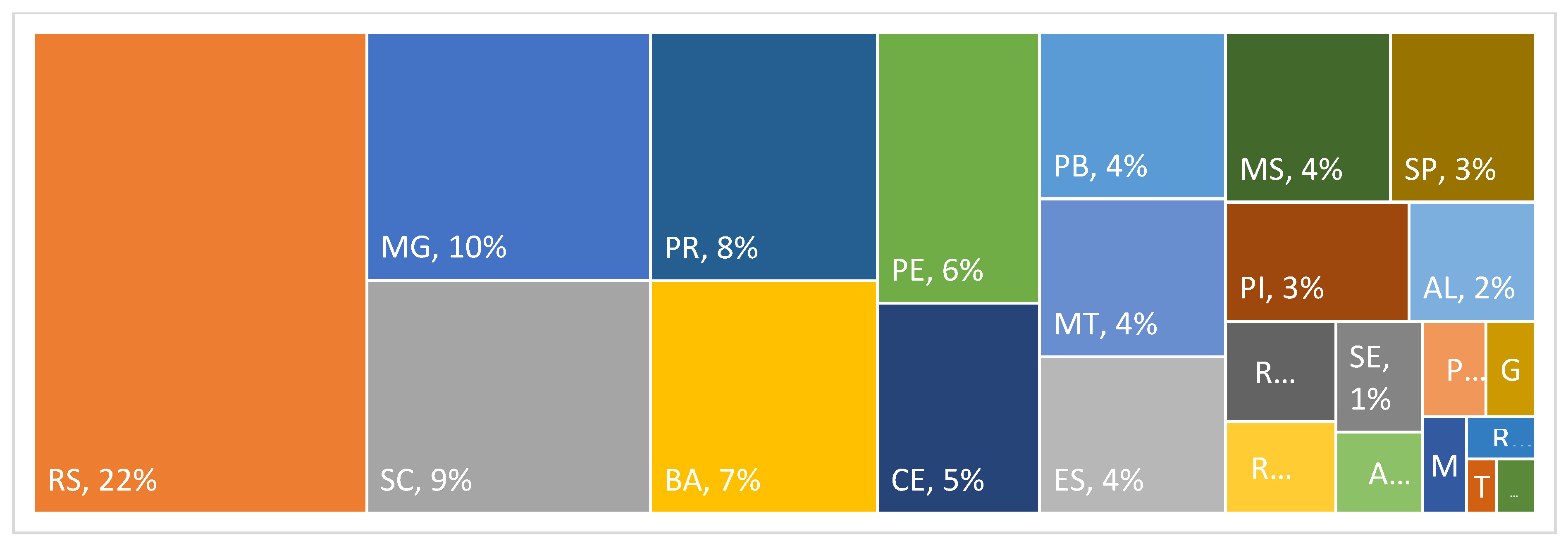
Figure 2.
Brazilian states: number of occurrences and losses (in billions), from 2000 to 2024. Source: Prepared by the authors. National Secretariat for Civil Defense and Protection—Sedec/MIDR—and the Center of Studies and Research in Engineering and Civil Defense—Ceped/UFSC. .
Figure 2.
Brazilian states: number of occurrences and losses (in billions), from 2000 to 2024. Source: Prepared by the authors. National Secretariat for Civil Defense and Protection—Sedec/MIDR—and the Center of Studies and Research in Engineering and Civil Defense—Ceped/UFSC. .
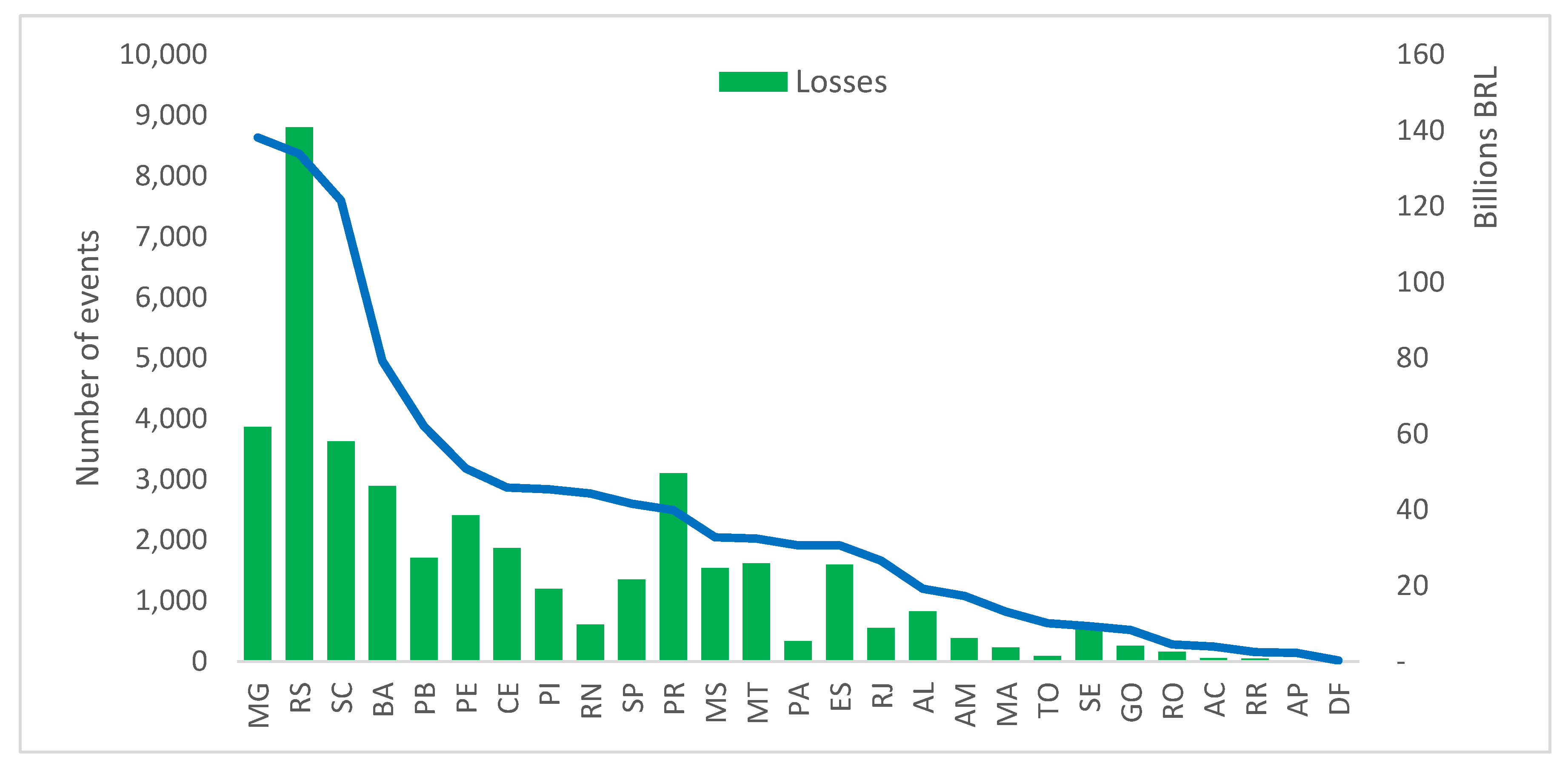
Figure 4.
Summary of analysis Methods. Source: Prepared by the authors.
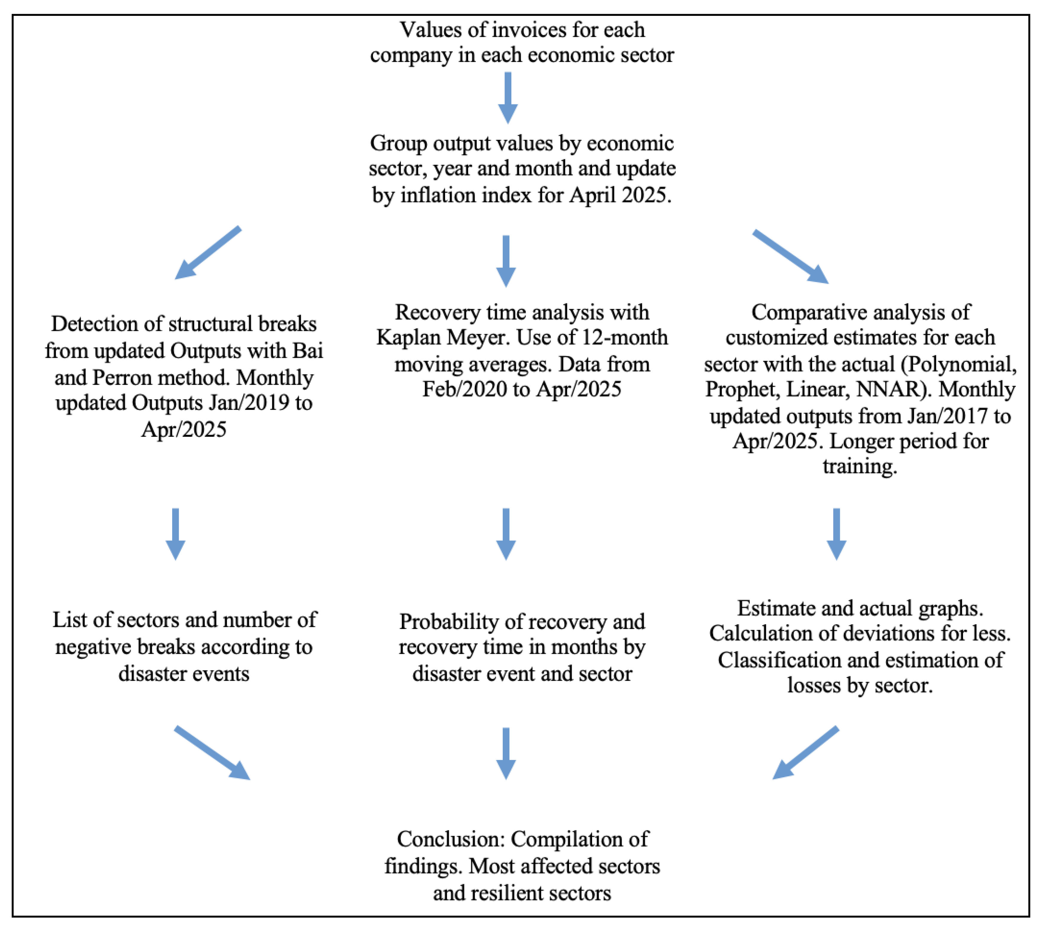
Figure 5.
Kaplan Meyer adaptada para os eventos. Source: Prepared by the authors.
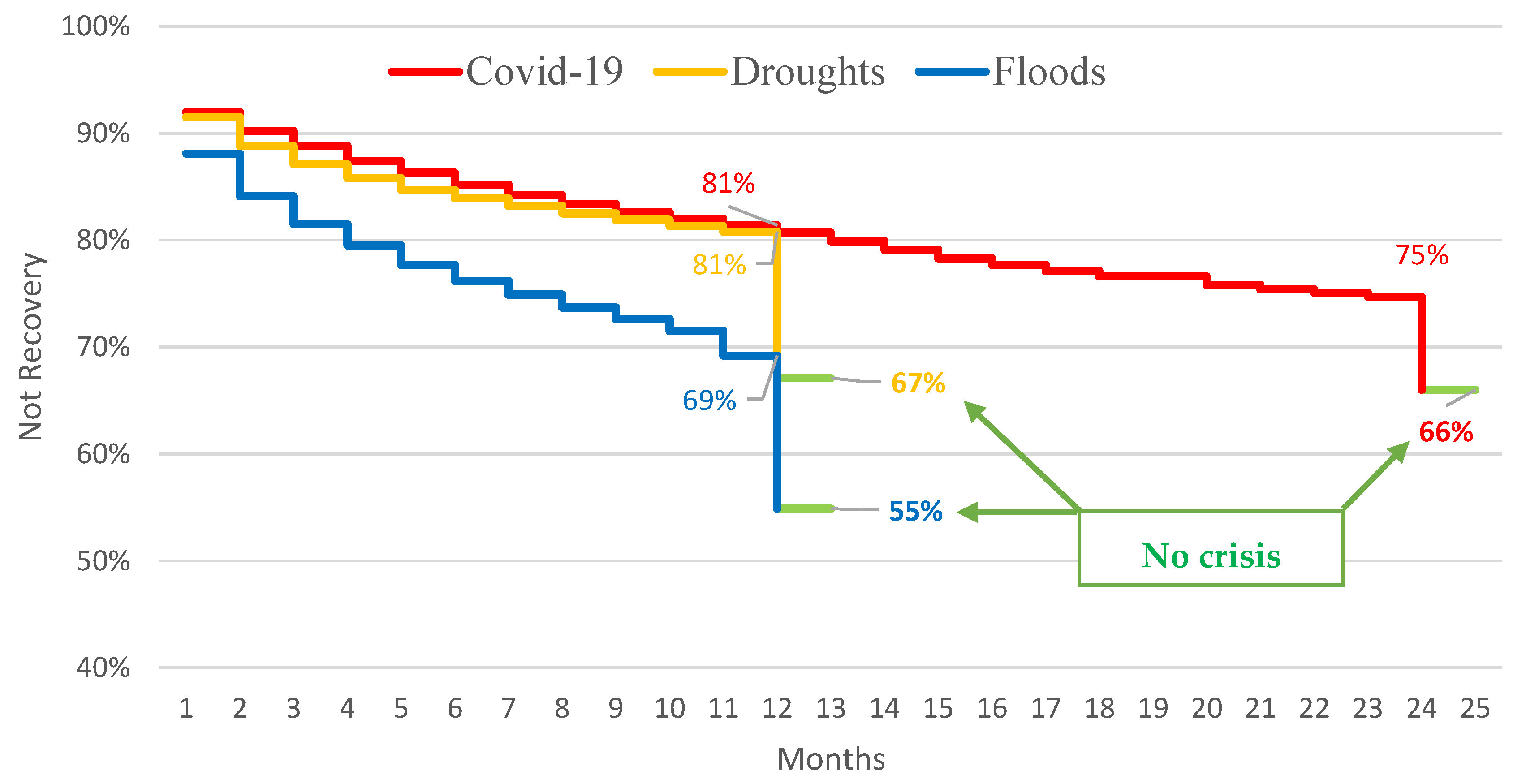
Figure 6.
Graph of the 16 largest sectors, estimated and actual from Jan/2020 to Apr/2025. Source: Prepared by the authors.
Figure 6.
Graph of the 16 largest sectors, estimated and actual from Jan/2020 to Apr/2025. Source: Prepared by the authors.
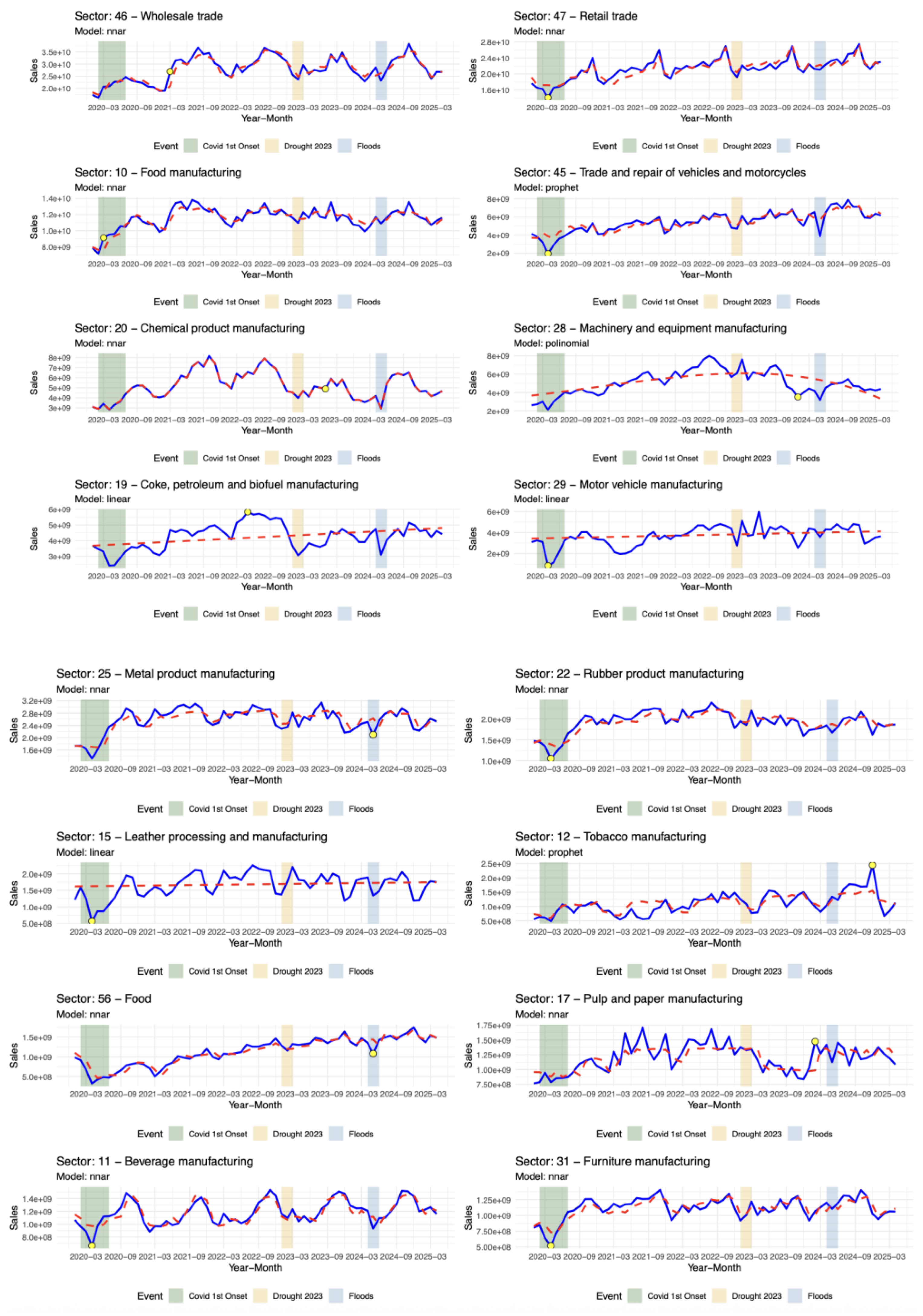

Table 1.
Main 18 economic sectors RS, average percentage in NF value from 2019 to 2024 and number of companies in 2024.
Table 1.
Main 18 economic sectors RS, average percentage in NF value from 2019 to 2024 and number of companies in 2024.
| Code | Sector | Average Perc. 2019-2024 |
Number of Companies 2024 | ||
|---|---|---|---|---|---|
| Standard | Simplified tax regime | Total | |||
| 46 | Wholesale trade, except motor vehicles and motorcycles | 26.52 | 7,617 | 7,322 | 14,939 |
| 47 | Retail trade | 20.68 | 23,559 | 73,093 | 96,652 |
| 10 | Manufacture of food products | 10.97 | 1,809 | 3,129 | 4,938 |
| 45 | Trade and repair of motor vehicles and motorcycles | 5.15 | 4,107 | 12,711 | 16,818 |
| 20 | Manufacture of chemical products | 4.95 | 478 | 356 | 834 |
| 28 | Manufacture of machinery and equipment | 4.69 | 1,037 | 1,129 | 2,166 |
| 19 | Manufacture of coke, petroleum products and biofuels | 4.09 | 23 | 4 | 27 |
| 29 | Manufacture of motor vehicles, trailers and bodies | 3.66 | 283 | 337 | 620 |
| 25 | Manufacture of metal products, exc. Machinery, equipment | 2.45 | 923 | 3,722 | 4,645 |
| 22 | Manufacture of rubber and plastic products | 1.85 | 661 | 816 | 1,477 |
| 15 | Preparation and manufacture of leather goods and footwear | 1.65 | 505 | 629 | 1,134 |
| 12 | Manufacture of tobacco products | 1.04 | 24 | 27 | 51 |
| 56 | Food | 1.07 | 2,012 | 14,573 | 16,585 |
| 17 | Manufacture of pulp, paper and paper products | 1.15 | 199 | 229 | 428 |
| 11 | Manufacture of beverages | 1.18 | 253 | 581 | 834 |
| 31 | Manufacture of furniture | 1.09 | 423 | 2,231 | 2,654 |
| 24 | Metallurgy | 1.18 | 104 | 143 | 247 |
| 35 | Electricity, gas and other utilities | 1.06 | 167 | 0 | 167 |
| Total | 94.41 | 44,184 | 121,032 | 165,216 | |
Source: Prepared by the authors.
Table 2.
Type of events that occurred in RS between 2000-2024, sum of updated value and number of incidences.
Table 2.
Type of events that occurred in RS between 2000-2024, sum of updated value and number of incidences.
| Event | Sum loss public and private | Frequency |
|---|---|---|
| Drought and dry spell | 99,991,029,811 | 3272 |
| Heavy rains | 16,877,598,521 | 1195 |
| Flash floods | 8,111,654,401 | 1408 |
| Floods | 5,866,260,674 | 529 |
| Windstorms and cyclones | 5,354,169,047 | 1080 |
| Hail | 3,809,812,126 | 654 |
| Flooding | 269,355,708 | 103 |
| Cold wave | 187,287,720 | 18 |
| Tornado | 160,653,724 | 31 |
| Others | 152,135,881 | 22 |
| Mass movement | 59,752,093 | 43 |
| Erosion | 10,999,763 | 2 |
| Forest fire | 6,816,583 | 7 |
| Dam failure | 1,746,494 | 2 |
| Infectious diseases | 17,797 | 2 |
| Heat wave and low humidity | 3,420 | 1 |
| Total geral | 140,859,293,762 | 8369 |
Source: Prepared by the authors. National Secretariat for Civil Defense and Protection—Sedec/MIDR—and the Center of Studies and Research in Engineering and Civil Defense—Ceped/UFSC. .
Table 3.
Descriptive statistics of variables.
| Variable | Description | Min | Median | Mean | Max |
|---|---|---|---|---|---|
| year | Year | 2017 | 2021 | 2021 | 2025 |
| month | Month | 1 | 6 | 6.392 | 12 |
| cod_firm | identification of the company | 0 | 17 | 58 | 979 |
| sector | sector national code | 0 | 47 | 42.93 | 97 |
| category | tax regime | regular | 3,933,169 | simplified | 11,431,954 |
| sai_nfe_nfc | Monthly value of sales invoices | 0 | 35,000 | 504,300 | 5,285,000,000 |
| IPCA | Inflation index | 1 | 1.288 | 1.268 | 1.518 |
Source: Prepared by the authors.
Table 4.
Sectors with structural breaks.
| Code | Sector | Breaks | Sector % |
|---|---|---|---|
| 26 | Manufacture of computer, electronic and optical equipment | 1 | 0,60% |
| 27 | Manufacture of electrical machinery, equipment and materials | 2 | 0,58% |
| 23 | Manufacture of non-metallic mineral products | 1 | 0,56% |
| 16 | Manufacture of wood products | 2 | 0,53% |
| 49 | Land transport | 3 | 0,45% |
| 32 | Manufacture of various products | 2 | 0,41% |
| 14 | Manufacture of clothing and accessories | 1 | 0,29% |
| 13 | Manufacture of textile products | 2 | 0,26% |
| 8 | Extraction of non-metallic minerals | 2 | 0,15% |
| 33 | Maintenance, repair and installation of machinery and equipment | 3 | 0,14% |
| 52 | Storage and auxiliary activities for transport | 2 | 0,12% |
| 38 | Collection, treatment and disposal of waste | 2 | 0,12% |
| 18 | Printing and reproduction of recordings | 2 | 0,09% |
| 21 | Manufacture of pharmaceutical and pharmaceutical products | 1 | 0,08% |
| 61 | Telecommunications | 2 | 0,07% |
| 43 | Specialized services for construction | 1 | 0,05% |
| 5 | Coal extraction | 2 | 0,04% |
| 58 | Publishing and integrated publishing with printing | 2 | 0,04% |
| 42 | Infrastructure works | 1 | 0,03% |
| 95 | Repair and maintenance of computer equipment | 2 | 0,02% |
| 20 sectors | 36 | 4.64% | |
| Other 26 sectors | 46 | 0.14% | |
| Total Breaks | 82 | 4,78% | |
| No breaks | 95,22% | ||
Source: Prepared by the authors.
Table 5.
Structural Breaks by event identification.
| Event | 2019 | 2020 | 2021 | 2022 | 2023 | 2024 | Total |
|---|---|---|---|---|---|---|---|
| Covid 1st Onset | 14 | 14 | |||||
| Covid 2nd Onset | 3 | 8 | 11 | ||||
| Covid 3rd Onset | 3 | 3 | |||||
| Covid 3rd Onset - Drought 2022 | 3 | 3 | |||||
| Drought 2023 | 3 | 3 | |||||
| Floods | 8 | 8 | |||||
| not detected | 4 | 3 | 11 | 11 | 10 | 1 | 40 |
| Total | 4 | 20 | 22 | 14 | 13 | 9 | 82 |
Source: Prepared by the authors.
Table 6.
Main Sectors, disaster and average time to recovery in months, only firms in crisis.
| Sectors | Covid-19 | Droughts | Floods | |||
| Perc. firms in crisis | Months | Perc. firms in crisis | Months | Perc. firms in crisis | Months | |
| Retail trade | 33% | 12.05 | 32% | 7.30 | 44% | 6.76 |
| Trade and repair of motor vehicles | 36% | 10.69 | 34% | 5.87 | 45% | 5.45 |
| Food | 30% | 14.62 | 21% | 6.27 | 38% | 7.03 |
| Wholesale trade | 35% | 10.03 | 35% | 7.03 | 48% | 6.39 |
| Manufacture of metal products | 41% | 8.66 | 44% | 6.40 | 52% | 5.80 |
| Food manufacturing | 37% | 11.43 | 30% | 6.96 | 44% | 6.95 |
| Manufacture of furniture | 43% | 9.22 | 47% | 6.32 | 52% | 5.07 |
| Manufacture of machines and equipment | 50% | 7.91 | 52% | 6.54 | 60% | 5.76 |
| Wood manufacturing | 46% | 9.01 | 49% | 6.46 | 58% | 5.79 |
| Clothing and accessories | 45% | 11.37 | 39% | 5.79 | 56% | 6.51 |
| Land transport | 21% | 9.78 | 26% | 6.13 | 36% | 5.64 |
| Average | 34% | 11.47 | 33% | 6.88 | 45% | 6.43 |
Source: Prepared by the authors.
Table 7.
Models and best adjustment.
| Model | Melhor ajuste | Descrição |
|---|---|---|
| Linear | 20 | Simple linear regression of Saidas_At as a function of time |
| Nnar | 38 | Autoregressive neural network for time series |
| Polinomial | 3 | 4th degree polynomial regression for complex curvatures |
| Prophet | 13 | Used for time series, with annual seasonality |
| Total of sectors | 74 |
Source: Prepared by the authors.
Table 8.
Resume of number of sectors with losses from 2020 to 2024.
| Item | 2020 | 2021 | 2022 | 2023 | 2024 |
|---|---|---|---|---|---|
| Number of sectors with losses | 54 | 24 | 21 | 44 | 43 |
| Resilient sectors | 20 | 50 | 53 | 30 | 31 |
| Average of losses in sectors with losses | -12% | -14% | -9% | -5% | -5% |
| Average 74 sectors | -8% | 0% | 3% | 0% | -1% |
Source: Prepared by the authors.
Table 9.
Performing of selected sectors.
| Sectors | 2020 | 2021 | 2022 | 2023 | 2024 |
|---|---|---|---|---|---|
| Travel agencies, tour operators and booking services | -27% | 4% | 2% | 18% | -8% |
| Agriculture, livestock and related services | -10% | 10% | 2% | -3% | -3% |
| Food | -7% | 2% | 3% | 2% | -2% |
| Accommodation | -9% | 4% | 3% | 5% | -7% |
| Artistic, creative and entertainment activities | -63% | -28% | 0% | 22% | 1% |
| Trade and repair of motor vehicles and motorcycles | -11% | 4% | 3% | -1% | 1% |
| Wholesale trade | -1% | 5% | 0% | -2% | 0% |
| Retail trade | -3% | 5% | 1% | -4% | 1% |
| Manufacture of clothing and accessories | -6% | 6% | 3% | 0% | -2% |
| Construction of buildings | -1% | -27% | -2% | -3% | 14% |
| Manufacture of beverages | -1% | -4% | 3% | 2% | 2% |
| Manufacture of machinery and equipment | -16% | 1% | 13% | 0% | -12% |
| Manufacture of machinery and materials electrical | 2% | 1% | 0% | -2% | 1% |
| Metallurgy | -1% | 2% | 0% | -1% | -1% |
| Household services | -20% | 8% | 10% | 18% | -8% |
Source: Prepared by the authors.
Disclaimer/Publisher’s Note: The statements, opinions and data contained in all publications are solely those of the individual author(s) and contributor(s) and not of MDPI and/or the editor(s). MDPI and/or the editor(s) disclaim responsibility for any injury to people or property resulting from any ideas, methods, instructions or products referred to in the content. |
© 2025 by the authors. Licensee MDPI, Basel, Switzerland. This article is an open access article distributed under the terms and conditions of the Creative Commons Attribution (CC BY) license (http://creativecommons.org/licenses/by/4.0/).
Copyright: This open access article is published under a Creative Commons CC BY 4.0 license, which permit the free download, distribution, and reuse, provided that the author and preprint are cited in any reuse.


