
Submitted:
28 July 2025
Posted:
30 July 2025
You are already at the latest version
Abstract
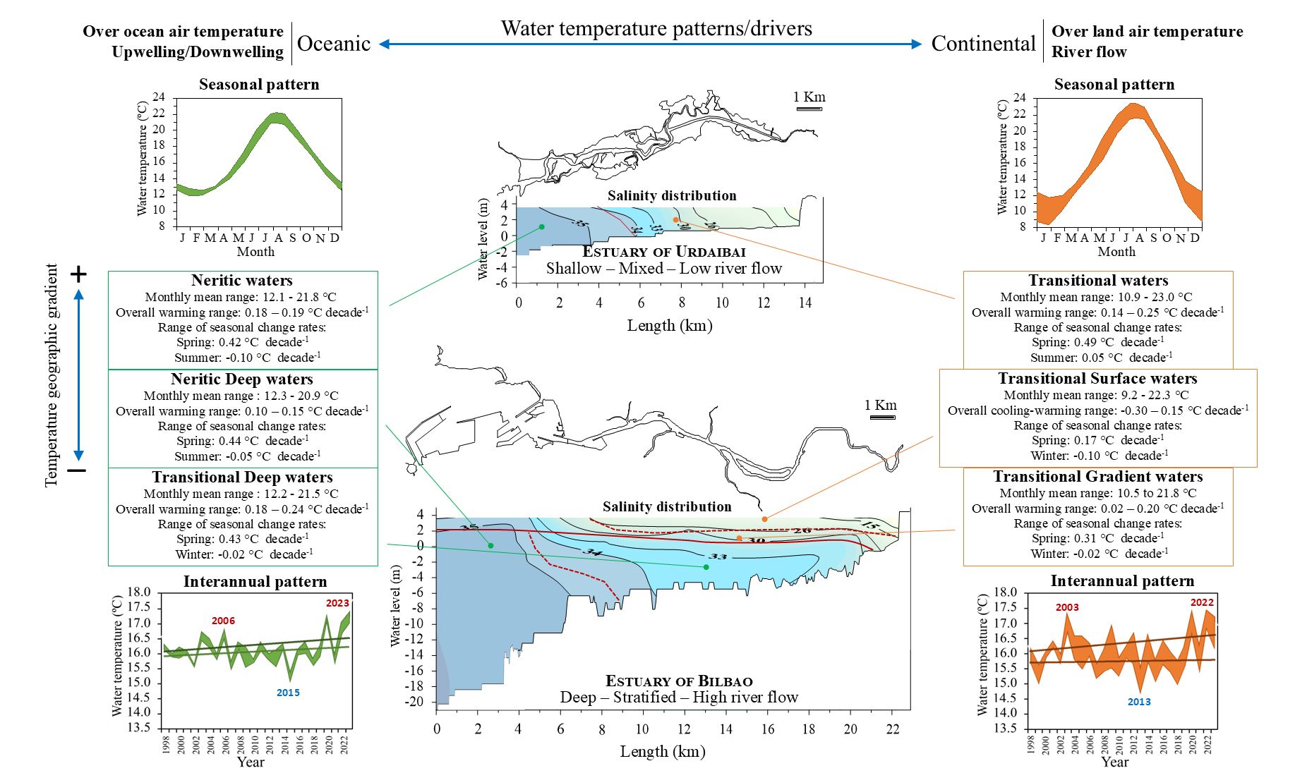
Temporal and spatial variations in water temperature were analysed from 23 time series across two contrasting Basque coast estuaries over a 26-year period (1998-2023). We examined long-term trends, seasonality, and intra- and inter-estuary variability, as well as links to local hydrometeorological factors and North Atlantic climate-ocean teleconnections. Time-series decomposition, clustering, and regression and correlation analyses were used. Water temperature interannual and seasonal patterns differed mainly between outer neritic waters and shallow transitional waters. Most water masses exhibited an overall warming trend, with temperature increases until 2003-2006, followed by declines until 2013-2015, and a sharp rise in 2020-2023, largely driven by spring temperatures. Warming was strongest (0.24-0.25 °C decade-1) in middle-estuary waters, while no trend or even cooling occurred in inner above-halocline waters of the stratified system. Spring, particularly May, experienced the highest warming rates, reaching 0.49 °C and 0.80 °C decade-1, respectively, in transitional waters of the mixed estuary. Seasonal temperature minima and maxima occurred earlier in surface transitional waters than in neritic waters and deep transitional waters of the stratified system. Over time, annual maxima advanced, minima were delayed, and spring temperatures rose, this extending the warm period. Air temperature, especially over-sea, was the primary driver of water temperature trends. River flow modulated the trends to annual and seasonal scales, inducing cooling, mainly in spring. AMO index was the teleconnection best related to water temperature, while links with the NAO index and the EA pattern were more restricted to specific seasons.
Keywords:
water temperature
; time series
; seasonality
; warming
; estuaries
; Bay of Biscay
1. Introduction
Temperature is a key driver of biological processes from molecular to ecosystem levels and varies over daily to multidecadal time scales. Much effort is being devoted to the development of theories and the prediction of biological responses to climate change across different levels of biological organization, and on different spatial and temporal scales [1,2,3]. A major focus of attention is the analysis of spatial and temporal temperature patterns in terrestrial and marine ecosystems in the context of the expected climate warming throughout the 21st century [4]. Globally, sea surface temperature (SST) is increasing [5], although there are some exceptions [6] and marked interregional differences in warming rates [7], which differ not only between ocean basins [8] but also at regional scales [9,10,11]. Coastal warming is highly heterogeneous, with temperature trends differing across continental shelves, and from coastal to open-ocean locations [12,13,14]. Beyond these systems, studies in Australia [15] and South Florida [16] have shown that estuarine waters are warming faster than adjacent shelf areas and at a greater rate than predicted by global ocean and atmospheric models, suggesting that these models may not accurately predict estuarine temperature trends [15]. A recent global assessment of estuarine surface water warming rates has shown that less than half of the studied estuaries have exhibited warming trends over the recent 30-yr period (1985-2022). Additionally, estuarine water warming trends have shown significant differences across hemispheres, continents, and between small and large estuaries [17].
Moreover, climate change affects not only mean SST trends but also variability, extreme values and seasonality, although these aspects remain less explored [6]. Models predict regional variability in SST warming in large marine systems such as the Baltic Sea, with clear latitude dependent seasonal warming differences [18,19]. Both predicted and observed water temperature changes also show spatial and seasonal differences in estuaries [20,21].
However, aquatic systems have a tridimensional structure and functioning, which cannot be shaped only from changes observed at surface. Studies on long-term water temperature variability with depth are more limited due to the scarcity of data at subsurface and bottom layers, but the existing evidence suggests that warming trends differ across depths, due to the influence of different forcing factors at each layer [22]. Similarly, the intensity, duration and spatial extension of heatwaves vary with water depth [23,24]. These differences are expected to be larger in coastal areas and estuaries, which are naturally prone to experiencing greater temperature fluctuations at smaller spatial (regional and local) and temporal scales than offshore environments, and therefore they are more likely to undergo increased ecological stress [25].
Estuaries are ecologically and economically valuable systems [26] but due to their high warming response to the current climate crisis [15,16], the biodiversity and uniqueness of estuarine biota, as well as the commercial and recreational services of estuaries are threatened. The rise in temperature is a common driver of water quality impairment in estuaries [27]. It can enhance the severity and extent of hypoxia [28] as well as the level of pathogens and infectious diseases [29], and increase the frequency, severity, and duration of harmful algal blooms [30]. Extreme thermal events can also affect fisheries, due to catastrophic fish mortality [31]. However, estuaries vary widely in size, morphology and hydrodynamics, and therefore encompass a broad range of vulnerabilities to climate warming [15]. Beyond atmospheric drivers, estuarine water temperature is affected by external factors such as upstream river temperature and discharge, marine water intrusions and coastal upwelling, as well as by internal processes such as mixing, dispersion, and water residence time e.g., [32,33,34,35]. This complexity in temperature patterns across spatial and temporal scales leads to different vulnerabilities to warming in the context of climate change, with implications for estuarine functions now and in the future [36]. Therefore, disentangling the spatial and temporal patterns and rates of temperature change in different types of estuaries and identifying their main driving factors is essential to improve our understanding of future environmental and biotic changes. Such insights are vital for informing management actions in these dynamic systems.
The aim of this study was to analyse water temperature variability at interannual and seasonal scales, as well as along axial and vertical spatial gradients, in two estuaries of the Basque coast, the estuary of Bilbao and the estuary of Urdaibai (Bay of Biscay), during the last 26-yr period (1998-2023). The specific objectives were the following
a) To identify distinct water mass clusters based on temperature variability similarities.
b) To describe long-term water temperature trends and assess rates of change.
c) To establish seasonal patterns, phenological changes, and seasonal and monthly differences in interannual temperature variations.
d) To determine the relationship of air temperature, river flow and upwelling events and the main climate teleconnections with water temperature variability at the different spatial and temporal scales studied.
e) To assess the role of estuarine morphology in shaping thermal conditions in the estuaries under study.
2. Materials and Methods
2.1. Study Area
The nearby estuaries of Bilbao (43° 23′ N, 03° 07′ W) and Urdaibai (43° 22’ N, 02° 43′ W) are located in the Basque coast (inner Bay of Biscay), within the eastern North Atlantic temperate region (Figure 1a). They share a temperate oceanic climate characterized by mild winters, warm summers, and frequent rainfall [37]. However, they differ largely in morphology, topography, and watershed characteristics [38]. The estuary of Bilbao is a highly man-modified system currently turned into an artificial channel 25 m wide and 0.5 m deep in the upper fluvial reaches, 270 m wide in the widest middle reaches and 10 m deep in the deepest lower reaches. This channel meets the Abra harbour, a semiconfined funnel-shaped embayment that increases in depth from around 12 m in the inner Abra to 32 m at the coastline (Figure 1b). Extensive land reclamation has greatly reduced intertidal areas, and dredging has deepened the estuary for navigation [39]. In contrast, the estuary of Urdaibai has remained much more natural, with an average depth of ~3 m at high tide and a greater proportion of intertidal and supratidal zones. However, a straight artificial channel was built alongside the natural meandering one in the upper estuary to facilitate navigation (Figure 1c).
Both estuaries experience a meso-macrotidal, semidiurnal tidal regime, but the estuary of Urdaibai has a much higher tidal prism volume/total volume ratio [40]. The estuary of Bilbao receives greater freshwater inflows, leading to a stratified system with a two-layer circulation [41] and a well-defined estuarine plume drifting offshore [42], whereas the estuary of Urdaibai is mostly a well-mixed system. Under usual river discharge conditions, both estuaries are sea-dominated systems with high salinity (euhaline > 30) water masses reaching the upper estuary below the halocline in the estuary of Bilbao and filling the outer half of the estuary of Urdaibai at high tide. However, the torrential nature of Basque coastal rivers [43] means that extreme flood events can for brief periods of time flush freshwater to the estuary mouths.
In the adjacent marine region, downwelling events prevail in autumn and winter due to southwesterly winds, while frequent episodes of weak upwelling occur in spring and summer under easterly and northeasterly winds [44].
2.2. Data Acquisition
Water temperature data were obtained from an ongoing hydrography and plankton monitoring program in the estuaries of Bilbao and Urdaibai. A Lagrangian sampling approach was used to assess changes in water masses of specific salinities instead of samplings at fixed locations. From 1998 to 2023, monthly measurements were taken at sites with salinities of 35, 34, 33, and 30 in the estuary of Bilbao and 35, 33, 30, and 26 in the estuary of Urdaibai, all of them below the halocline. These salinity sites were selected based on the axial distribution of water masses, ranging from the main salinity habitat (~35 salinity) for neritic plankton to brackish plankton habitats at varying salinities in each estuary. At each sampling site, water temperature was measured at 0.5 m intervals from just below the surface (where the sensor became submerged; hereafter referred to as surface (0.0 m)) to the bottom using different multiparameter meters (WTW and YSI) during the study period. To minimize tidal currents interference and short-term physical stressor variability, sampling was conducted, whenever possible, in the morning, close to the high tide slack, and during the second neap tide of the month.
To account for local influences, air temperature data for the marine area adjacent to the estuaries were obtained from the Copernicus Climate Data Store (https://cds.climate.copernicus.eu/datasets). Additionally, air temperature over land was sourced from three hydrometeorological stations (Figure 1a): Sondika (https://www.aemet.es), located between the basins of the two estuaries; Abusu (https://www.euskalmet.euskadi.eus/hasiera/), near the head of the estuary of Bilbao; and Muxika (https://www.euskalmet.euskadi.eus/hasiera/), near the head of the estuary of Urdaibai. River flow data were also obtained from the latter two gauging stations (https://www.uragentzia.euskadi.eus/), representing the combined flow of the Ibaizabal and Nerbioi rivers in the estuary of Bilbao and the Oka river in the estuary of Urdaibai. Upwelling index data were accessed from the Spanish Institute of Oceanography (http://www.indicedeafloramiento.ieo.es/interactivo.html).
Finally, teleconnection indices (NAO: North Atlantic Oscillation, EA: East Atlantic pattern, AMO: Atlantic Multidecadal Oscillation, and AO: Arctic Oscillation) were obtained from the NOAA Climate Prediction Center (https://www.cpc.ncep.noaa.gov/).
2.3. Data Selection
23 water temperature time series (combinations of sites and depths) were used for the present study. The selected temperature measurements included surface (0.0 m) and 2.5 m depths at all salinity sites in both estuaries, and 5.0 m and 7.5 m depths at all salinity sites in the estuary of Bilbao except for 30 salinity at 7.5 m, where this depth was generally unavailable. Due to the shallowness of the estuary of Urdaibai, data below 2.5 m were not consistently available. Similarly, in the estuary of Bilbao, measurements at 5.0 m and 7.5 m were occasionally missing due to shallow water depths or cable length limitation (8 m) of the multiparameter meter used until 2003. To fill these gaps at some depths, missing values were primarily replaced with values from the depth nearest to the missing depth. Likewise, for other occasional missing data, two gap-filling methods were applied: 1) When a predefined salinity was not found, or temperature data were missing due to instrument failure (overall <4.5%), missing values of temperature were estimated from polynomial regression models of temperature variation as a function of salinity. To this purpose data from other sampling sites of the same date were used; 2) When a sampling was cancelled, missing values were estimated using the average of the preceding and following sampling dates (< 2.5%).
Finally, the criterion to establish the months included in each season was that the three coldest and three warmest consecutive months in the highest salinity time series are winter and summer, respectively. As a result, January, February and March were considered as winter, April, May and June as spring, July, August and September as summer and October, November and December as winter.
2.4. Data Processing
First, the interannual trend component of the 23 water temperature time series, the afore mentioned local hydrometeorological factors and the teleconnection indices were extracted using the multiple seasonal decomposition function (mstl) from the forecast v.8.21 package in R [45].
According to similarities in interannual trends, the 23 water temperature time series were grouped into six distinct water mass clusters using Ward's hierarchical clustering method, based on Spearman’s rank correlation (r = 0.8), with clusters defined at a 0.3 height threshold. For each sampling date, mean temperatures were calculated for each cluster of time series. To identify breakpoints in the variations of these mean temperatures throughout the study period, a Cumulative Sum (CuSum) analysis was conducted for each water mass cluster.
Additionally, the monthly mean for the entire study period were calculated for each water temperature time series to establish the standard seasonal pattern.
Linear regression analysis was performed to estimate temperature change rates per decade and assess their statistical significance in the trend component of each water temperature time series. The same analysis was applied to temperature data for each water mass cluster split by seasons.
Finally, Spearman rank correlation analyses were conducted to explore relationships between water temperature and local environmental factors and North Atlantic climate teleconnections.
All statistical analyses were performed by means of R software [46].
3. Results
3.1. Water Temperature Time-Series Clustering
Hierarchical clustering analysis of the 23 water temperature time series identified six water mass clusters based on similarities in interannual trends (Figure 2) herein termed as:
1) BTD (Bilbao-Transitional-Deep). It includes time series from the intermediate and inner (transitional) waters of the estuary of Bilbao, specifically from below the halocline (deep). This water mass cluster comprises data from 2.5, 5.0, and 7.5 m depths at the 34 salinity site, 5.0 and 7.5 m at the 33 salinity site, and 5.0 m at the 30 salinity site.
2) UN (Urdaibai-Neritic). It includes time series from the neritic waters of the 35 salinity site (both surface and 2.5 m depths) of the estuary of Urdaibai.
3) BND (Bilbao-Neritic-Deep). It includes time series from the outer zone (neritic) of the estuary of Bilbao, specifically from below the halocline (deep). This group comprises data from 2.5, 5.0 and 7.5 m at the 35 salinity site.
4) UT (Urdaibai-Transitional). It includes time series from the transitional waters of the estuary of Urdaibai, comprising data from surface and 2.5 m depths at the 33, 30, and 26 salinity sites.
5) BTS (Bilbao-Transitional-Surface). It includes time series from the intermediate and inner (transitional) surface waters of the estuary of Bilbao. The group comprises data from 0.0 m depth at the 34, 33, and 30 salinity sites.
6) BTG (Bilbao-Transitional-Gradient). It is a mixed group from the estuary of Bilbao, which includes the time series from the 35 salinity site at surface and the 33 and 30 salinity sites at 2.5 m depth.
Figure 2.
Similarity dendrogram of water temperatures from the 23 time series, constructed using Ward's hierarchical clustering method based on Spearman's rho correlations. Water masses (see text for definition of BTD, UN, BND, UT, BTS and BTG waters) are defined by a 0.3 height threshold (dotted line), with water clusters outlined by boxes.
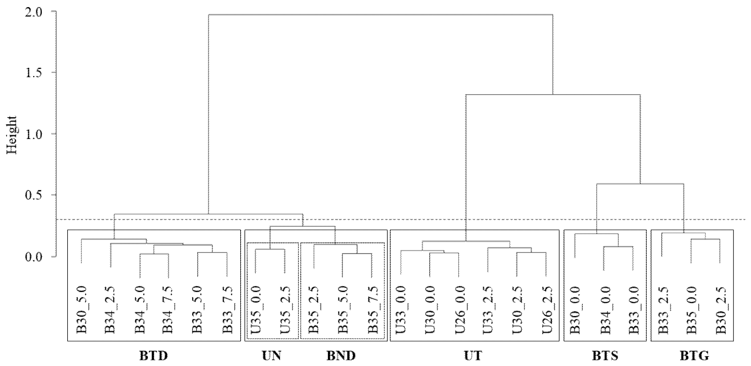
As shown in Figure 2, BND and UN were grouped into a single cluster at the set threshold and therefore they included data from both estuaries. However, this was an exception, as the rest of groups were related to a single estuary. Therefore, it was decided to treat BND and UN as separate clusters. At a lower similarity level, BTD merged with the neritic assemblage (BND and UN), while the other transitional waters (UT, BTS, and BTG) formed a separate group.
3.2. Interannual Trends in Water Temperature Across Water Masses
Interannual trends of water temperature at each depth, salinity site and estuary showed an overall significant increase in most cases during the study period (Figure 3 and Table 1).
Exceptions were observed in some surface waters of the estuary of Bilbao, where a clear downward trend (-0.3 °C decade-1 at the 30 salinity site) or no trend (at the 33 and 35 salinity sites) was found. The strongest increases were observed at the 26 salinity site in the UT water masses and at the 33 salinity site in the BTD ones, with warming rates of 0.25 °C and 0.24 °C decade-1, respectively. Additionally, UN waters showed a slightly higher increase (0.18-0.19 °C decade-1) than BND ones (0.10-0.15 °C decade-1).
However, the increase was not gradual. Water temperature trend showed a decrease across all time series from 2003-2006 to 2013-2015, followed by an increase in the last years of the study period. In addition, the warmest and coldest years varied between clusters. Annual mean values for each water mass (cluster) showed that 2023 was the warmest year in neritic waters (UN and BND) and 2022 in transitional waters (UT, BTG, BTS). In the first half of the study period temperature peaked in 2006 in neritic waters and 2003 in transitional waters. The coldest years were 2015 in neritic waters and 2013 in transitional waters. Temperature in BTD waters (nearest ones to the neritic waters of the estuary of Bilbao) were an exception because they aligned better with the neritic pattern (Figure 3).
The CuSum analysis of water temperature data calculated for the six water mass clusters (Figure 4) revealed five distinct periods: 1) 1998-2002, characterized by values below the mean in the main water masses (UN, BND, BTD, and UT); 2) 2003-2006, with values above the mean, especially in the earliest years in UT, BTG, and BTS, and in later years in BND, UN, and BTD; 3) 2007-2012, with values below the mean but closer to it in UT, BTG, and BTS waters; 4) 2013-2019, characterized by the lowest values below the mean across all waters; and 5) 2020-2023, with values significantly above the mean.
The linear interannual trends and the periods of increase and decrease identified by the CuSum analysis primarily reflected the interannual patterns of spring (April-June) water temperature, which showed stronger variations and higher rates of increase than other seasons temperatures (Figure 5 and Table 2). Indeed, spring showed the strongest warming across all water masses, with UT showing the largest spring increase (0.49 °C decade-1) and BTS waters the smallest one (0.17 °C decade-1). Autumn also showed considerable warming (0.28 to 0.22 °C decade-1 in UN, UT and BTD clusters).
In contrast, summer and winter displayed greater variability, with summer showing both warming (e.g., in BTD waters 0.23 °C decade-1) and cooling (e.g., minimum rise in UN waters: -0.10 °C decade-1), while winter had the most inconsistent patterns, with predominantly negative trends. However, none of these relationships were statistically significant. Similarly, the interannual rates of change of water temperature at the monthly scale (Figure 6) were positive for all spring months, with May showing the strongest rates across most water masses (0.88 °C decade-1 in UT, and between 0.5 and 0.6 °C decade-1 in BND, BTD, and UN). In autumn months, highest rates were observed in November or December (e.g. 0.63 °C decade-1 in December in UT). Negative change rates were primarily observed in summer and winter months, especially in August for UN (-0.37 °C decade-1) and in March for BTS (-0.60 °C decade-1).
3.3. Seasonal Patterns in Water Temperature Across Water Masses
Overall, as depth and salinity increased, winter temperatures were higher, summer temperatures lower, and the annual temperature range narrowed (Figure 7). An exception was observed in the estuary of Bilbao, where summer maxima were higher at the surface of the 33 salinity site compared to the 30 salinity site. Also, the estuary of Urdaibai showed higher temperatures at the same depths and salinity sites than the estuary of Bilbao. The ranges of average water temperatures of each water mass cluster (Figure 7) were the following: from 12.2-12.4 to 20.6-21.1 °C in BND waters, from 12.0-12.2 to 21.7-21.8 °C in UN ones, from 11.9-12.4 to 21.0-21.9 °C in BTD ones, from 10.1-11.6 to 22.5-23.4 °C in UT ones, and from 8.4-10.9 to 21.5-22.6 °C for the joint BTG plus BTS waters.
The timing of the annual water temperature minima and maxima, as well as the coldest and warmest periods varied between the different water masses. Coldest periods occurred from January to March, with annual minima in February for the BND, UN, and BTD waters, while for BTS and UT ones the coldest periods were from December to February, with annual minima in January. Annual maxima were skewed toward July in UN, UT and BTS waters (Figure 7). Spring water temperatures were always higher than autumn temperatures, with the smallest differences observed in deep water masses of the estuary of Bilbao (BND and BTD), and the highest in inner surface ones (BTS) (Figure 7). In the estuary of Urdaibai, such seasonal differences were also found from UN to UT waters with an increase in the difference between spring and autumn temperatures and decreases in the temperature difference between spring and summer, and between autumn and winter.
In all water masses temperature seasonality (Figure 8) was similar in the five time periods identified by the CuSum analysis. The most significant variation over time of the annual cycle was the delay of the coldest winter values towards March and the advance of the warmest summer values towards July, which led to a shortening of the seasonal warming period (although this process did not occur in a totally gradual manner). The delay of the winter minima was more evident in the neritic waters of both systems and the transitional waters of the estuary of Urdaibai, where a faster and greater warming from April to May was also observed in the last period (2020-2023). In contrast, the first period (1998-2002) showed the lowest May temperatures and the coldest springs in all water masses, except in BTS ones. The 2003-2006 period was characterized by the coldest winters (at least in January and February or February and March) in all water masses and warmest summers (except in BTD waters), and therefore, the highest temperature ranges. The 2007-2012 time span showed the coldest autumns in all water masses. The 2013-2019 period was characterized by water temperatures below the time series mean for all the seasons in all water masses, and by the lowest range of temperature variation between the warmest and coldest periods. In contrast, the 2020-2023 period showed water temperatures above the time series mean for all the seasons, with warmest springs and autumns in all water masses, warmest winters in UN, BND and BTD, and warmest summers in BTD.
3.4. Relationship of Water Temperature with Local Environmental Factors and Climate Teleconnections
Interannual trends of local environmental factors and teleconnection indices showed a significant increase over the study period (Figure 9 and Table 3). Regarding air temperatures, the rate of change varied considerably across meteorological station sources (Table 3).
At the monthly scale (Figure 10), warming rates were quite similar between over-land and over-ocean air temperature data. The assessment of the month specific rate of warming/cooling showed an overall increasing trend of warming rates from winter (with decreasing rates in January) to autumn, with highest warming rates in November-December. Similarly, at the monthly scale, river flow trends showed an almost coincident seasonal pattern between basins; with increasing rates in late autumn and early winter (from November to February) and clear decreasing rates in early spring (March-April) and early autumn (October). The upwelling index showed a somewhat opposite pattern to that of river flow, with a marked increase in April and October but a decline in January.
Regarding the relationship between environmental factors and water temperature (Table 4), air temperature showed the highest positive correlations across all cases, with over ocean air temperature data (ATc) being the most consistent. However, over-land-air temperatures showed stronger correlations during winter and/or summer in some water masses, the air temperature measured at the head of the estuaries (ATa/m) being the most strongly correlated factor with water temperature in all transitional water masses (BTD, UT, BTG and BTS). River flow showed significant negative correlations, except during the summer in the estuary of Urdaibai (UN and UT) and below the halocline in the estuary of Bilbao (BND and BTD), where no correlations were observed. The upwelling index was positively correlated with water temperature in spring in all water masses. In contrast, overall teleconnection indices showed fewer and less significant correlations. AMO index showed significant positive correlations with temperature in all water masses and generally in most seasons except summer. Negative correlations were found for NAO index, but only in autumn. EA pattern only correlated with water temperature in summer in deep waters of the estuary of Bilbao (BND and BTD), and in winter in non-deep transitional waters (UT, BTG and BTS). Positive correlations with AO were only observed for BTD and BTG in winter.
4. Discussion
4.1. Differences in Thermal Environments
Water masses differed between and within estuaries in their interannual variability, seasonal pattern and range of temperature. Neritic waters of both estuaries showed a very similar pattern, likely influenced by the connectivity of waters along the adjacent coastal area. However, the thermal features of transitional waters responded differently in each estuary depending on the water circulation and mixing patterns, which are shaped by the morphology of the estuaries and the river discharges. The higher river discharge and deeper water column generate vertical stratification in the estuary of Bilbao, and this causes differences in thermal features between surface and deeper transitional waters. The deep transitional waters in the estuary of Bilbao are formed by the intrusion of high-salinity marine water that flows landwards [41]. The limited air temperature and river flow influences allow these waters to retain a neritic thermal behaviour, as shown in the present work. The surface transitional waters, however, exhibited a different thermal environment due to the persistence and extent of the stratification that allowed a greater influence of air temperatures. In contrast, under conditions of low river discharge and shallowness, mixing dominates in the estuary of Urdaibai and a similar thermal behaviour over the entire column was observed, influenced also by air temperatures. The distinction between the neritic thermal environment and the thermal environments of transitional waters in both estuaries agrees with the differentiation of water masses due to the dominance of neritic and brackish zooplankton species, respectively [38,47]. The thermal differences we found followed a spatial pattern commonly observed in estuaries, where upper reaches are consistently warmer than the lower estuary [33]. However, results also revealed that the main waters of the estuary of Bilbao were, on average, colder and more thermally stable than those in the estuary of Urdaibai. This implies differences in the thermal habitats of brackish communities in each estuary, which could partly explain the observed between-estuary differences in the dominance and phenology of the main zooplankton brackish species [48].
4.2. Overall Trends and Change Rates
Water temperature increased during the 1998-2023 period in all the water masses, except for the lowest-salinity above-halocline waters of the inner estuary of Bilbao, where it decreased. Our data further suggests that warming trends may reverse if poorly mixed freshwater masses expand at surface towards lower reaches if river flows increase. In estuaries, freshwater discharge generally affects upper layers more than bottom layers, and freshwater runoff can influence the magnitude and spatial distribution of heating or cooling rates, especially in frontal areas [49]. This agrees with observations in the present study, where the correlation between water temperature and river flow was higher in transitional gradient waters than in bottom or inner surface transitional waters during the rainiest seasons in the stratified estuary of Bilbao. As observed in our study, sites within estuaries that deviate from the prevailing warming trend have been reported from many other estuaries [50,51]. Both of our systems showed the highest warming in transitional waters, with rates of 0.25-0.24 °C decade-1 (considering data from all months in the series). The average warming rate from 1998 to 2023 in the main transitional waters of these two estuaries (0.21 °C decade-1) was lower than the average increase of 0.37 °C decade-1 reported for all modelled English estuaries between 1990 and 2022 [51]. However, our series lacks the colder years registered in the early 90’s (as shown by SST data from the nearby Aquarium of San Sebastian [52], which may bias the comparison towards lower warming rates. Nonetheless, interregional differences between our south-eastern Bay of Biscay estuaries and English estuaries are smaller than the intraregional differences (0.70-0.05 °C decade-1) reported for the latter [51]. The higher warming rates in transitional water masses compared to the average 0.15 °C decade-1 in neritic waters of our two systems is in agreement with the idea that estuaries are more sensitive to global warming than open sea waters [15,16]. Our results, however, also evidenced that warming rates in neritic waters decreased substantially from surface layers in the estuary of Urdaibai (0.19 °C decade-1) to subsurface layers in the estuary of Bilbao (0.13 °C decade-1). This is very likely due to the combined effect of depth and the west to east gradient of temperature increase that develops in the inner Bay of Biscay during the warm period [11]. In fact, in the Bay of Biscay the southeastern corner has shown the strongest warming trend [53], and our two neritic sites have shown progressively lower rates westward, but lower than the 0.23 °C decade-1 SST rate of change obtained further east along the Basque coast from 1980 to 2019 [54]. However, as mentioned above, this comparison must be taken with caution due to the lack of data from the 80’s and most years of the 90`s in our series. The surface layer of neritic water masses in the estuary of Bilbao showed a thermal behaviour different from that of the subsurface layers. Similarly, in the more vertically homogeneous shelf waters, spatial and temporal differences in warming have been identified at contrasting depths [22].
4.3. Trends and Change Rates at Intra-Annual Scales
In our systems, the interannual trends and rates of change of seasonal and monthly water temperatures showed strongest warming in spring (April to June), lower in autumn (November/December), and lowest or even cooling trends in summer (August) and winter (February/March). This pattern is consistent with observations in the Bay of Biscay from 1982 to 2014 [11]. This latter study reported higher warming trends from September to November and from April to June and lower SST increases from January to March and from July to August. However, the seasonal and monthly rates of change they recorded (range: > 0.3 °C decade-1 to < 0.2 °C decade-1) were smaller than those in our two systems indicating that, while intra-annual variations in water temperature trends at our local scale are in accordance with the regional patterns, in the nearshore-inshore waters rates of change are higher.
Our results also confirm that warming was mainly driven by an extended warm season rather than milder winters or warmer summers [11]. This pattern appears to characterize the first quarter of the 21st century in the Bay of Biscay, but it does not match observations during the last decades of the 20th century. For example, during the 1965-2004 period, [55] reported a clear seasonal dependence of warming rates, with summer temperature trends being twice as strong as those of winter in surface waters. In the southeastern Bay of Biscay, from 1972 to 1993, both winter and summer showed warming trends, but the winter increase was slightly higher [53]. Likewise, along the Cantabrian coast, spring and summer showed similar warming trends from 1985 to 2005 [56]. Results from other marine (e.g. NW Mediterranean [57]; northeastern continental shelf of North America [13]) and estuarine areas (e.g. Yangtze River Estuary [21]; Hudson River Estuary [58]; South Florida estuaries [16]) further confirm that seasonal variations in water temperature trends and rates of change can vary greatly as a function of the time-window and sites/areas analysed. Overall, these differences highlight the need for joint analysis of water temperature series from different regions and time periods to better understand the spatial and temporal effects of climate change in coastal and transitional systems.
4.4. Interannual Patterns
The alternation of warming and cooling periods identified in our systems, with inflexion points in 2003-2006 and 2013-2015, matched the large scale subpolar North Atlantic SST trend reversal from warming (1994-2004) to cooling (2005-2015) [59]. Earlier and longer (from 1965 to 2004) water temperature data from 0 to 100 m depth in the Bay of Biscay also showed an overall, though non steady, warming during 1965-2004, when an initial cooling period occurred until the early 1970s [55]. A six-decade (1947-2007) SST analysis from a coastal location close to our study area identified cycles of approximately 8, 11, and 18 years, linked to climate cycles [52]. These alternating cooling-warming trends in the Bay of Biscay were more patent during the first decade of the 2000s (2002-2014) under atmospheric conditions favourable for plume enhancement [60]. Our results support the relationship between cooling and increased river discharge, but overall, the cooling-warming cycles also coincide with broader spatial scale cycles that affect the Bay of Biscay and the temperate Atlantic region. Regarding extreme temperatures, in the cooling-warming cycles in neritic waters we identified the warm summer values of 2020 and 2023 and the cold winter values of 2015, in addition to the warm summer values of 2003 and 2006 and the cold winter values of 2005. This timing for the maximum and minimum values was also observed for the SST series from a more eastward site on the Basque coast [52].
4.5. Seasonal Patterns
The largest difference in seasonal patterns was observed between neritic subsurface waters of the estuary of Bilbao and surface waters of the inner estuary of Bilbao, and it seemed to be mostly due to the dominant oceanic and continental influence respectively. This difference involved larger temperature variations in the shallower waters located landwards from the mouth, a pattern observed in other estuaries too e.g., [61]. Annual water temperature minima were lowest and most skewed towards January in above-halocline waters of the estuary of Bilbao and transitional shallow waters of the estuary of Urdaibai. In contrast, in neritic and below-halocline waters of the estuary of Bilbao, minima were milder and skewed towards March, as in the adjacent coastal/shelf waters of the Cantabrian Sea [56]. However, no such differences were observed for the annual maximum values and their timing. A similar pattern has been reported in other European marine areas, including the Baltic Sea, where summer SST peaks in August, but winter minima occur in February in shallow waters and in March in deeper areas [62]. Seasonal patterns also showed interannual differences. Throughout the study period, the seasonal warming phase shortened due to a delay in winter minima, an advance in summer maxima, and an earlier start of an extended warm period. This pattern agrees with observations of trends made at a broader spatial scale across the North Atlantic in recent decades. These data have shown that despite the timing of the spring warming transition has remained constant from 1998 to 2022, there are small areas that have experienced either delayed or advanced transitions, such as the earlier spring warming transition registered in the Bay of Biscay [63]. Similarly, SST trends in the North American northeastern continental shelf showed earlier summer onset and longer durations between 1982 and 2014 [13].
4.6. Relationships with Local Climate and Hydrographic Factors
In our two systems, at the interannual scale air temperature was the main driver of water temperature variability. In addition, warming rates in transitional waters (0.25-0.24 °C decade-1) were comparable to trends in offshore air temperatures from the Copernicus database. However, overall, the waters (neritic and transitional) of both estuaries warmed more slowly than air temperature. In contrast, Chesapeake Bay showed faster warming of some estuarine waters than of air temperature, particularly in the main stem [50], while the Hudson estuary showed no significant difference between air and water temperature increases [58]. However, the seasonal patterns of air and water temperature from our two systems showed differences, which suggests that local factors modulate estuarine water warming responses. Unlike air temperature, spring (April-June) water temperature showed strong warming trends. A similar pattern was reported for the Hudson River estuary, where water warming maximum occurred in April-August but air temperature one in December and February-March [58].
Despite differences in river flow between estuaries, the overall trend of increase in freshwater discharge had a cooling effect on water temperature in both systems, which was reflected in a decline until 2013–2015, followed by a rise as river discharges first increased and then decreased. A similar cooling influence of freshwater discharge has been reported for the Bay of Biscay during 1982-2014, where river-influenced areas cooled while offshore waters warmed [60]. In the present study, the highest cooling effect was observed in above-halocline water masses of the inner estuary of Bilbao. However, responses of water temperature to river discharge and air temperature vary across estuaries. For example, in the Hudson River estuary increased freshwater input did not counteract water warming related to the increase in air temperature [58], while in the San Francisco Bay-Delta system, the combined effects of atmospheric and riverine influences differed spatially [34]. In our study, water temperature correlated strongly with river flow in spring and autumn, but no relationship was found in summer. Similarly, in the upper San Francisco Estuary, the negative relationships between water temperature and river inflow were most common, although positive relationships were found, in winter [35].
Significant positive correlations between water temperature and upwelling index were found across all water-masses in the estuaries of Bilbao and Urdaibai, but only in spring. Spatial differences in SST show that regions in the SW Bay of Biscay experiencing intense upwelling show lower SST values [53] and coastal upwelling mitigates warming in nearshore waters in comparison to adjacent ocean waters along the western Iberian Peninsula [12,64]. Upwelling and downwelling events also shape the thermohaline properties of the northwestern Iberian estuaries [32,65]. In our study, downwelling was the dominant process, and it showed a weakening trend (upwelling index increased), that was most intense in April; accordingly, as stated above, we only found a significant positive correlation between upwelling index and temperature in spring. This interannual pattern is opposite to what we would expect if upwelling/downwelling had a dominant effect on SST e.g., [66,67,68]. Coastal upwelling and downwelling processes are driven by local atmospheric forces, and on the Basque coast, the seasonal pattern shows that spring downwelling relaxation is related to reduced wind stress and changes in wind direction, mainly of the prevailing northwesterly winds [40]. This suggest that water temperature trends in our estuaries may be influenced more by changes in more local winds than by shelf water advective processes. Surface water warming can be influenced by both atmospheric surface heat flux and oceanic horizontal thermal advection, with winds playing a significant role in air-water heat flux [69] (Pei et al., 2017). However, studies report positive, negative and uncertain relationships between SST and surface wind speed in coastal waters e.g., [69,70,71,72]. Therefore, the effect of winds on water temperature in our study area remains unclear, highlighting the need to include wind data in future analyses of water temperature variability.
4.7. Relationships with Climate Teleconnections
The AMO index showed the most consistent relationship with interannual temperature variations across all water masses and seasons in both estuaries. According to [73], the AMO has been the dominant teleconnection pattern in the Bay of Biscay, i.e. it has explained the highest percentage of interannual SST variability, over a recent period of 150 years, while the influence of the NAO and EA patterns has been smaller and limited to specific years or shorter periods. In our study, the AMO was always positively correlated with water temperature in spring and autumn, the two seasons with the highest warming rates, while the NAO was correlated inversely only with autumn temperature. This contrasts with observations from coastal areas of the Bay of Biscay located northwards from our study sites and influenced by river plumes, where SST was positively correlated with the NAO index between 1982 and 2014 [60]. However, it agrees with the sequential negative correlation of the NAO index with air temperature and the positive correlation between air temperature and water temperature obtained in our study area from 1997 to 2005 [74]. Such change of sign in the relationship between NAO and SST across the Bay of Biscay might be due to the transitional position of this marine region between the northern and southern European centres, which exhibit opposite temperature responses to the NAO index [75]. On the North American northeastern continental shelf, SST change trends also show regionally variable links to the NAO index [13]. In our sites the EA and OA patterns showed weaker relationships with water temperature overall and seasonally. However, the positive relationships obtained in our study area are consistent with findings from nearby areas, where the positive phase of the EA was linked to increased incidence, duration, and intensity of marine heatwaves in a central coastal area of the Cantabrian Sea (SW Bay of Biscay) between 1998 and 2019 [76].
5. Conclusions
Our results reveal common patterns in water temperature variability across both estuaries, which agree with those observed over wider areas in the Cantabrian Sea, the Bay of Biscay, and the North Atlantic. However, differences between and within estuaries highlight the sensitivity of estuaries to climate warming in a global context, as well as, to the specific features that characterize the Basque coast. Based on temperature ranges and seasonal and interannual variability, two main thermal behaviours were identified. One is associated with water masses from the estuary mouths (neritic) and below the halocline in the stratified estuary of Bilbao, which was characterized by lower temperature variability, later annual minima and an interannual delay in the alternation of warmest and coldest events influenced by shelf waters thermal properties and dynamics. The other one is linked to water masses in the intermediate-inner reaches of the estuary of Urdaibai and surface waters of the estuary of Bilbao, which showed a higher variability and a stronger influence of local land-atmosphere conditions.
Temperature trends showed similar maximum warming rates in transitional water masses of both estuaries, but in different water masses, because these maxima were observed in below-halocline higher salinity waters (euhaline) in the estuary of Bilbao and in shallow lower salinity waters (polyhaline) in the estuary of Urdaibai. Warming rates were higher in the neritic waters of the estuary of Urdaibai than in the estuary of Bilbao, likely due to between-estuary differences in depth and geographic location. Overall, decreasing trends in above-halocline inner waters of the estuary of Bilbao were linked to river discharge and over-land climate factors.
Highest warming rates occurred in spring, particularly in May, except for the above-halocline waters of the estuary of Bilbao, likely due to the higher influence of river discharge in these waters. The strongest cooling in August sharpened summer negative trends in the neritic waters of both estuaries. A similar pattern was observed in winter in the above-halocline waters of the estuary of Bilbao. These cooling trends were attributed to external factors of marine and continental origin, respectively. A delay in the coldest annual temperatures and an advance in the warmest ones, which shortened the annual warming period, were the main water temperature phenological changes. Additionally, a sharp increase in May extended the warm period, reflecting a transition from cooler to warmer conditions over the study period.
Water temperature was primarily driven by air temperature but modulated by river flow, which had a cooling impact, particularly in spring and autumn. The relationship between upwelling index and temperature was complex, suggesting the influence of additional factors.
Teleconnection patterns showed the AMO index had the most consistent relationship with temperature, especially in waters with higher influence of marine waters (neritic waters and below-halocline waters of the estuary of Bilbao), while the NAO was mainly linked to autumn temperatures. The EA and AO had weaker associations with temperature changes.
Author Contributions
Conceptualization, F.V.; methodology, I.U.; software, I.U. and G.B.; validation, I.U. and F.V.; formal analysis, I.U., X.L. and G.B.; investigation, I.U.; resources, I.U., F.V. and A.I.; data curation, , I.U., X.L. and G.B.; writing—original draft preparation, F.V.; writing—review and editing, I.U., F.V., G.B. and A.I.; visualization, I.U., F.V. and A.I.; supervision, F.V. and A.I.; project administration, F.V. and A.I.; funding acquisition, F.V. All authors have read and agreed to the published version of the manuscript.
Funding
This research was funded by the Basque Government (PIBA2020-1-0028 & IT1723-22).
Data Availability Statement
Data will be made available at a reasonable request.
Acknowledgments
We also thank the High Technical School of Navigation of the Faculty of Engineering in Bilbao (UPV/EHU) for the facilities offered to carry out the field work.
Conflicts of Interest
The authors declare no conflicts of interest.
References
- Waldock, C.; Dornelas, M.; Bates, A.E. Temperature-driven biodiversity change: disentangling space and time. BioScience 2018, 68, 873–884. [Google Scholar] [CrossRef]
- Bütikofer, L.; Anderson, K.; Bebber, D.P.; Bennie, J.; Early, R.; Maclean, I.M.D. The problem of scale in predicting biological responses to climate. Glob. Change Biol. 2020, 26, 6657–6666. [Google Scholar] [CrossRef] [PubMed]
- Arroyo, J.I.; Díez, B.; Kempes, C.P.; West, G.B.; Marquet, P.A. A general theory for temperature dependence in biology. Proc. Natl. Acad. Sci. U.S.A. 2022, 119(30), e2119872119. [CrossRef]
- Di Cecco, G.J.; Gouhier, T.C. Increased spatial and temporal autocorrelation of temperature under climate change. Sci. Rep. 2018, 8, 14850. [CrossRef]
- Hartmann, D.L.; Klein-Tank, A.M.G.; Rusticucci, M.; Alexander, L.V.; Bronnimann, S.; Charabi, Y.; Dentener, F.J.; Edlugokencky, E.J.; Easterling, D.R.; Kaplan, A.; Soden, B.J.; Thorne, P.W.; Wild, M.; Zhai, P. Observations: Atmosphere and Surface, in The Physical Science Basis. In Contribution of Working Group I to the Fifth Assessment Report of the Intergovernmental Panel on Climate Change; Stocker, T.F.; Qin, D.; Plattner G.-K.; et al.; Eds; Cambridge University Press, Cambridge, United Kingdom, 2013; pp. 159-254.
- Alexander, M.A.; Scott, J.D.; Friedland, K.D.; Mills, K.E.; Nye, J.A.; Pershing, A.J.; Thomas, A.C. Projected sea surface temperatures over the 21st century: Changes in the mean, variability and extremes for large marine ecosystem regions of Northern Oceans. Elementa-Sci. Anthrop. 2018, 6, 9. [CrossRef]
- Lee, M.A.; Huang, W.P.; Shen, Y.L.; Weng, J.S.; Semedi, B.; Wang, Y.C.; Chan, J.W. Long term observations of interannual and decadal variation of sea surface temperature in the Taiwan Strait. J. Mar. Sci. Tech. 2021, 29, 7. [CrossRef]
- Levitus, S.; Antonov, J.I.; Boyer, T.P. Warming of the World Ocean, 1955-2003. Geophys. Res. Lett. 2005, 32, L02604. [Google Scholar] [CrossRef]
- Ginzburg, A.I.; Kostianoy, A.G.; Sheremet, N.A. Seasonal and interanual variability of the Black Sea surface temperature as revealed from satellite data (1982-2000). J. Mar. Syst. 2004, 52, 33–50. [Google Scholar] [CrossRef]
- Santos, A.M.P.; Kazmin, A.S.; Peliz, A. Decadal changes in the Canary upwelling system as revealed by satellite observations: Their impact on productivity. J. Mar. Res. 2005, 63, 359–379. [Google Scholar] [CrossRef]
- Costoya, X.; Decastro, M.; Gómez-Gesteira, M.; Santos, F. Changes in sea surface temperature seasonality in the Bay of Biscay over the last decades (1982–2014). J. Mar. Syst. 2015, 150, 91–101. [Google Scholar] [CrossRef]
- Santos, F.; Gómez-Gesteira, M.; deCastro, M.; Álvarez, I. Variability of coastal and ocean water temperature in the upper 700 m along the western Iberian Peninsula from 1975 to 2006. PLOS ONE 2012, 7(12), e50666. [CrossRef]
- Thomas, A.; Pringle, P.; Pfleiderer, P.; Schleussner, C.F. Tropical cyclones: impacts, the link to climate change and adaptation. Climate Analytics, 2017, Nov. 6. (PDF) Climate Change and Small Island Developing States. Available online: https://climateanalytics.org/publications/tropical-cyclones-impacts-the-link-to-climate-change-and-adaptation/.
- Varela, R.; de Castro, M.; Días, J.M.; Gómez-Gesteira, M. Coastal warming under climate change: Global, faster and heterogeneous. Sci. Total Environ. 2023, 15, 886, 164029. [CrossRef]
- Scanes, E.; Scanes, P.R.; Ross, P.M. Climate change rapidly warms and acidifies Australian estuaries. Nat. Commun. 2020, 11, 1803. [Google Scholar] [CrossRef]
- Shi, J.; Hu, Ch. South Florida estuaries are warming faster than global oceans. Environ. Res. Lett. 2023, 18, 014003. [CrossRef]
- Prum, P.; Harris, L.; Gardner, J. Widespread warming of Earth's estuaries. Limnol. Oceanogr. Lett. 2024, 9, 268–275. [Google Scholar] [CrossRef]
- BACC Lead Author Group. Assessment of Climate Change for the Baltic Sea Basin. International BALTEX secretariat. 2006. Available online: http://www.gkss.de/baltex/publications/PubNo_35/IBS%20No35%20BACC.pdf.
- Meier, H.E.M. Baltic Sea climate in the late 21st century - A dynamical downscaling approach using two global models and two emission scenarios. Clim. Dyn. 2006, 27, 39–68. [Google Scholar] [CrossRef]
- Brown, C.; Sharp, D.; Mochon Collura, T.C. Effect of climate change on water temperature and attainment of water temperature criteria in the Yaquina estuary, Oregon (USA). Estuar. Coast. Shelf Sci. 2016, 169, 136–146. [Google Scholar] [CrossRef]
- Wang, J.; Wang, J.; Xu, J.; Yang, Y.; Lyv, Y.; Luan, K. Seasonal and interannual variations of sea surface temperature and influencing factors in the Yangtze River Estuary. Reg. Stud. Mar. Sci. 2021, 45, 101827. [Google Scholar] [CrossRef]
- Friedland, K.D.; Morse, R.E.; Manning, J.P.; Melrose, D.C.; Miles, T.; Goode, A.G.; Brady, D.C.; Kohut, J.T.; Powell, E.N. Trends and change points in surface and bottom thermal environments of the US Northeast Continental Shelf Ecosystem. Fish. Oceanogr. 2020, 29, 396–414. [Google Scholar] [CrossRef]
- Fernández-Barba, M.; Huertas, I.E.; Navarro, G. Assessment of surface and bottom marine heatwaves along the Spanish coast. Ocean Model. 2024, 190, 102399. [Google Scholar] [CrossRef]
- Lien, V.S.; Raj, R.P.; Chatterjee, S. Surface and bottom marine heatwave characteristics in the Barents Sea: a model study. In 8th edition of the Copernicus Ocean State Report (OSR8); von Schuckmann, K.; Moreira, L.; Grégoire, M.; Marcos, M.; Staneva, J.; Brasseur, P.; Garric, G.; Lionello, P.; Karstensen, J.; Neukermans, G.; Eds; Copernicus Publications, State Planet, 4-osr8, 8, 2024. [CrossRef]
- Wolowicz, M.; Sokołowski, A.; Lasota, R. Estuaries - a biological point of view. Oceanol. Hydrobiol. Stud. 2007, 36, 113–130. [Google Scholar] [CrossRef]
- Thrush, S.F.; Townsend, M.; Hewitt, J.E.; Davies, K.; Lohrer, A.M.; Lundquist, C.; Cartner, K. The many uses and values of estuarine ecosystems. In Ecosystems services in New Zealand- conditions and trends; Dymond, J.R.; Eds; Manaaki Whenua Press, New Zealand, 2014; pp. 226-237.
- US EPA, 2006. Oregon Water Quality Assessment Report. Available online: http://iaspub.epa.gov/waters10/attains_state.control?p_state.OR&p_cycle.2006.
- Rabalais, N.N.; Turner, R.E.; Díaz, R.J.; Justic, D. Global change and eutrophication of coastal waters. ICES J. Mar. Sci. 2009, 66, 1528–1537. [Google Scholar] [CrossRef]
- Burge, C.A.; Eakin, C.M.; Friedman, C.S.; Froelich, B.; Hershberger, P.K.; Hofmann, E.E.; Petes, L.E.; Prager, K.C.; Weil, E.; Willis, B.L.; Ford, S.E.; Harvell, C.D. Climate change influences on marine infectious diseases: implications for management and society. Ann. Rev. Mar. Sci. 2014, 6, 249–77. [Google Scholar] [CrossRef] [PubMed]
- Moore, S.K.; Trainer, V.L.; Mantua, N.J.; Parker, M.S.; Laws, E.A.; Backer, L.C.; Fleming, L.E. Impacts of climate variability and future climate change on harmful algal blooms and human health. Environ. Health 2008, 7(2), S4. [CrossRef]
- Blewett, D.A.; Stevens, P.W. Temperature variability in a subtropical estuary and implications for common snook Centropomus undecimalis, a cold-sensitive fish. Gulf Mex. Sci. 2014, 32, 44–54. [Google Scholar] [CrossRef]
- Alvarez, I.; Gomez-Gesteira, M.; deCastro, M.; Prego, R. Variation in upwelling intensity along the NorthWest Iberian Peninsula (Galicia). J. Atmos. Ocean Sci. 2005, 10, 309–324. [Google Scholar] [CrossRef]
- Wooldridge, T.; Deyzel, S. Variability in estuarine water temperature gradients and influence on the distribution of zooplankton: a biogeographical perspective. Afr. J. Mar. Sci. 2012, 34, 465–477. [Google Scholar] [CrossRef]
- Vroom, J.; van der Wegen, M.; Martyr-Koller, R.C.; Lucas, L.V. What determines water temperature dynamics in the San Francisco Bay-Delta system? Water Resour. Res. 2017, 53, 9901–9921. [Google Scholar] [CrossRef]
- Bashevkin, S.M.; Mahardja, B. Seasonally variable relationships between surface water temperature and inflow in the upper Sa Francisco Estuary. Limnol. Oceanogr. 2022, 67, 684–702. [Google Scholar] [CrossRef]
- Gross, P.L.; Gan, J.C.L.; Scurfield, D.J.; Frank, C.; Frank, C.; McLean, C.; Bob, C.; Moore, J.W. Complex temperature mosaics across space and time in estuaries: implications for current and future nursery function for Pacific salmon. Front. mar. sci. 2023, 10, 1278810. [Google Scholar] [CrossRef]
- Usabiaga, J.I.; Sáenz-Aguirre, J.; Valencia, V.; Borja, A. Climate and meteorology, variability and its influence on the ocean. In Oceanography and marine environment of the Basque Country; Borja, A.; Collins, M.; Eds.; Elsevier Oceanography Series 70. Elsevier, Amsterdam, 2004; pp. 75-95.
- Barroeta, Z.; Uriarte, I.; Iriarte, A.; Villate, F. Intraregional variability of exotic and native zooplankton in Basque coast estuaries (inner Bay of Biscay): effect of secondary dispersion, estuary features and regional environmental gradients. Hydrobiologia 2024, 851, 667–687. [Google Scholar] [CrossRef]
- Cearreta, A.; Irabien, M.J.; Pascual, A. Human activities along the Basque coast during the last two centuries: geological perspective of recent anthropogenic impact on the coast and its environmental consequences. In Oceanography and marine environment of the Basque Country; Borja, A.; Collins, M.; Eds.; Elsevier Oceanography Series 70. Elsevier, Amsterdam, 2004; pp. 27-50.
- Valencia, V.; Borja, A.; Franco, J.; Galparsoro, I.; Tello, E. Medio físico y dinámica de los estuarios de la costa vasca. aplicaciones en ecología y gestión. 2024. Departamento de Ordenación del Territorio y Medio Ambiente, Gobierno Vasco.
- Uriarte, I.; Villate, F.; Iriarte, A.; Duque, J.; Ameztoy, I. Seasonal and axial variations of net water circulation and turnover in the estuary of Bilbao. Estuar. Coast. Shelf Sci. 2014, 150, 312–324. [Google Scholar] [CrossRef]
- Fernández-Nóvoa, D.; Costoya, X.; deCastro, M.; Gómez-Gesteira, M. Dynamic characterization of the main Cantabrian river plumes by means of MODIS. Cont. Shelf Res. 2019, 183, 14–27. [Google Scholar] [CrossRef]
- Uriarte, A.; Collins, M.; Cearreta, A.; Bald, J.; Evans, G. Sediment supply, transport and deposition: contemporary and Late Quaternary evolution. In Oceanography and marine environment of the Basque Country; Borja, A.; Collins, M.; Eds.; Elsevier Oceanography Series 70. Elsevier, Amsterdam, 2004; pp. 97-131.
- Fontán, A.; Valencia, V.; Borja, Á.; Goikoetxea, N. Oceano-meteorological conditions and coupling in the southeastern Bay of Biscay, for the period 2001–2005: A comparison with the past two decades. J. Mar. Syst. 2008, 72, 167–177. [Google Scholar] [CrossRef]
- Hyndman, R.; Athanasopoulos, G.; Bergmeir, C.; Caceres, G.; Chhay, L.; O'Hara-Wild, M.; Petropoulos, F.; Razbash, S.; Wang, E.; Yasmeen, F. Forecast: Forecasting functions for time series and linear models. R package version 8.21. 2023. Available online: https://pkg.robjhyndman.com/forecast/.
- R Core Team. R: A Language and Environment for Statistical Computing. R Foundation for Statistical Computing, Vienna, Austria. 2024. Available online: https://www.R-project.org/.
- Barroeta, Z.; García, T.; Uriarte, I.; Iriarte, A.; Villate, F. Response of native and non-indigenous zooplankton to inherent system features and management in two Basque estuaries: a niche decomposition approach. Estuar. Coast. Shelf Sci. 2022, 272, 107878. [Google Scholar] [CrossRef]
- Barroeta, Z.; Villate, F.; Uriarte, I.; Iriarte, A. Differences in the colonization success and impact of non-indigenous and other expanding copepod species on the zooplankton of two contrasting estuaries of the Bay of Biscay. Biol. Invasions 2020, 22, 3239–3267. [Google Scholar] [CrossRef]
- Shen, H.; Zhu, Y.; He, Z.; Li, L.; Lou, Y. Impacts of river discharge on the sea temperature in Changjiang estuary and its adjacent sea. J. Mar. Sci. Eng. 2022, 10, 343. [Google Scholar] [CrossRef]
- Ding, H.; Elmore, A.J. Spatio-temporal patterns in water surface temperature from Landsat time series data in the Chesapeake Bay, U.S.A. Remote Sens. Environ. 2015, 168, 335–348. [Google Scholar] [CrossRef]
- Hutchings, A.M.; De Vries, C.S.; Hayes, N.R.; Orr, H.G. Temperature and dissolved oxygen trends in English estuaries over the past 30 years. Estuar. Coast. Shelf Sci. 2024, 306, 108892. [Google Scholar] [CrossRef]
- Goikoetxea, N.; Borja, Á.; Fontán, A.; González, M.; Valencia, V. Trends and anomalies of sea surface temperature during the last 60 years, within the southeastern Bay of Biscay. Cont. Shelf Res. 2009, 29, 1060–1069. [Google Scholar] [CrossRef]
- Koutsikopoulos, C.; Beillois, P.; Leroy, C.C.; Taillefer, F. Temporal trends and spatial structures of the sea surface temperature in the Bay of Biscay. Oceanol. Acta 1998, 21, 335–344. [Google Scholar] [CrossRef]
- Chust, G.; González, M.; Fontán, A.; Revilla, M.; Alvarez, P.; Santos, M.; Cotano, U.; Chifflet, M.; Borja, A.; Muxika, I.; Sagarminaga, Y.; Caballero, A.; de Santiago, I.; Epelde, I.; Liria, P.; Ibaibarriaga, L.; Garnier, R.; Franco, J.; Villarino, E.; Irigoien, X.; Fernandes-Salvador, J.A.; Uriarte, A.; Esteban, X.; Orue-Echevarria, D.; Figueira, T.; Uriarte, A. Climate regime shifts and biodiversity redistribution in the Bay of Biscay. Sci. Total Environ. 2022, 803, 149622. [Google Scholar] [CrossRef] [PubMed]
- Michel, S.; Treguier, A.M.; Vandermeirsch, F. Temperature variability in the Bay of Biscay during the past 40 years, from an in situ analysis and a 3D global simulation. Cont. Shelf Res. 2009, 29, 1070–1087. [Google Scholar] [CrossRef]
- Gómez-Gesteira, M.; deCastro, M.; Álvarez, I.; Gesteira, J.L.G. Coastal sea surface temperature warming trend along the continental part of the Atlantic Arc (1985-2005). J. Geophys. Res. 2008, 113, C04010. [Google Scholar] [CrossRef]
- Salat, J.; Pascual, J.; Flexas, M.; Chin, T.M.; Vazquez-Cuervo, J. Forty-five years of oceanographic and meteorological observations at a coastal station in the NW Mediterranean: a ground truth for satellite observations. Ocean Dyn. 2019, 69, 1067–1084. [Google Scholar] [CrossRef]
- Seekell, D.A.; Pace, M.L. Climate change drives warming in the Hudson River Estuary, New York (USA). J. Environ. Monit. 2011, 13, 2321–2327. [Google Scholar] [CrossRef]
- Piecuch, C.G.; Ponte, R.M.; Little, C.M.; Buckley, M.W.; Fukumori, I. Mechanisms underlying recent decadal changes in subpolar North Atlantic Ocean heat content. J. Geophys. Res. 2017, 122, 7181–7197. [Google Scholar] [CrossRef]
- Costoya, X.; Fernandez-Novoa, D.; deCastro, M.; Santos, F.; Lazure, P.; Gomez-Gesteira, M. Modulation of sea surface temperature warming in the Bay of Biscay by Loire and Gironde Rivers. J. Geophys. Res. Oceans 2016, 121, 966–979. [Google Scholar] [CrossRef]
- Marin, M.J.; Sutherland, D.A.; Helms, A.R. Water temperature variability in the Coos Estuary and its potential link to eelgrass loss. Front. mar. sci. 2022, 9, 930440. [Google Scholar] [CrossRef]
- Bradtke, K.M.; Herman, A.; Urbanski, J.A. Spatial and interannual variations of seasonal sea surface temperature patterns in the Baltic Sea. Oceanologia 2010, 52, 345–362. [Google Scholar] [CrossRef]
- Friedland, K.D.; Nielsen, J.M.; Record, N.R.; Brady, D.C.; Morrow, C.J. The phenology of the spring phytoplankton bloom in the North Atlantic does not trend with temperature. Elem. Sci. Anth. 2024, 12(1), 00111. [CrossRef]
- Piedracoba, S.; Pardo, P.C.; Álvarez-Salgado, X.A.; Torres, S. Seasonal, interannual and long-term variability of sea surface temperature in the NW Iberian upwelling, 1982-2020. J. Geophys. Res. Oceans 2024, 129, e2024JC021075. [Google Scholar] [CrossRef]
- Alvarez, I.; Días, J.M.; DeCastro, M.; Vaz, N.; Sousa, M.C.; Gómez-Gesteira, M. Influence of upwelling events on the estuaries of the north-western coast of the Iberian Peninsula. Mar. Freshw. Res. 2013, 64, 1123–1134. [Google Scholar] [CrossRef]
- Barton, E.D.; Largier, J.; Torres, R.; Sheridan, M.; Trasviña, A.; Souza, A.; Pazos, Y.; Valle-Levinson, A. Coastal upwelling and downwelling forcing of circulation in a semi-enclosed bay: Ria de Vigo. Prog. Oceanogr. 2015, 134, 137–189. [Google Scholar] [CrossRef]
- Goela, P.C.; Cordeiro, C.; Danchenko, S.; Icely, J.; Cristina, S.; Newton, A. Time series analysis of data for sea surface temperature and upwelling components from the southwest coast of Portugal. J. Mar. Syst. 2019, 163, 12–22. [Google Scholar] [CrossRef]
- Gramer, L.J.; Zhang, J.A.; Alaka, G.J.; Hazelton, A.T.; Gopalakrishnan, S.G. Coastal downwelling intensifies landfalling hurricanes. Geophys. Res. Lett. 2022, 49(13), e2021GL096630. [CrossRef]
- Pei, Y.H.; Liu, X.H.; He, H.L. Interpreting the sea surface temperature warming trend in the Yellow Sea and East China Sea. Sci. China Earth Sci. 2017, 60, 1558–1568. [Google Scholar] [CrossRef]
- Yeh, S.-W.; Kim, C.-H. Recent warming in the Yellow/East China Sea during winter and the associated atmospheric circulation. Cont. Shelf Res. 2010, 30, 1428–1434. [Google Scholar] [CrossRef]
- Qu, B.; Gabric, A.J.; Zhu, J.; Lin, D.; Qian, F.; Zhao, M. Correlation between sea surface temperature and wind speed in Greenland Sea and their relationships with NAO variability. Water Sci. Eng. 2012, 5, 304–315. [Google Scholar] [CrossRef]
- El-Geziry, T.M.; Elbessa, M.; Tonbol, K. On the relationships between sea surface temperature and atmospheric conditions over the southern Levantine basin. Egypt. J. Aquat. Biol. Fish. 2023, 27, 203–216. [Google Scholar] [CrossRef]
- García-Soto, C.; Pingree, R.D. Atlantic Multidecadal Oscillation (AMO) and sea surface temperature in the Bay of Biscay and adjacent regions. J. Mar. Biol. Assoc. U. K. 2012, 92, 213–234. [Google Scholar] [CrossRef]
- Aravena, G.; Villate, F.; Iriarte, A.; Uriarte, I.; Ibañez, B. Influence of the North Atlantic Oscillation (NAO) on climatic factors and estuarine water temperature on the Basque coast (Bay of Biscay): Comparative analysis of three seasonal NAO indices. Cont. Shelf Res. 2009, 29, 750–758. [Google Scholar] [CrossRef]
- Castro-Díez, Y.; Pozo-Vázquez, D.; Rodrigo, F.S.; Esteban-Parra, M.J. NAO and winter temperature variability in southern Europe. Geophys. Res. Lett. 2002, 29, 1-1-1-4. [Google Scholar] [CrossRef]
- Izquierdo, P.; Rico, J.M.; González, F.; González, R.; Arrontes, J.M. Characterization of marine heatwaves in the Cantabrian Sea, S Bay of Biscay. Estuar. Coast. Shelf Sci. 2022, 274, 107923. [Google Scholar] [CrossRef]
Figure 1.
a) Geographic location of the estuaries of Bilbao and Urdaibai, with map of the estuary watersheds and location of hydrometeorological stations (Abusu (a), Sondika (s), and Muxika (m)) also indicated. b) Shape of the estuaries of Bilbao (left) and Urdaibai (right). c) Boxplots of salinity at selected depths for each sampled salinity site throughout the study period in the estuary of Bilbao (left) and Urdaibai (right).
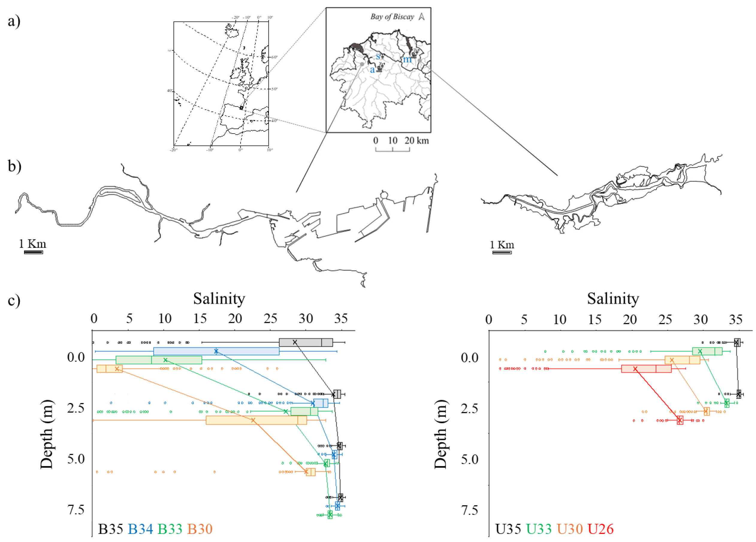
Figure 3.
Variation in the trend component of water temperature in the estuaries of Urdaibai (U) and Bilbao (B) at the studied sites (35, 34, 33, 30 and 26 salinity) and depths (0.0, 2.5, 5.0 and 7.5 m from surface), that conformed the water masses obtained in the cluster analysis (see Figure 2), throughout the study period. Straight lines represent the linear adjustment (regression parameters detailed in Table 1). Circles indicate the annual means for the water mass. Warmest years for the first and second half of the study period are shown in red, and the coldest one across the study period in blue.
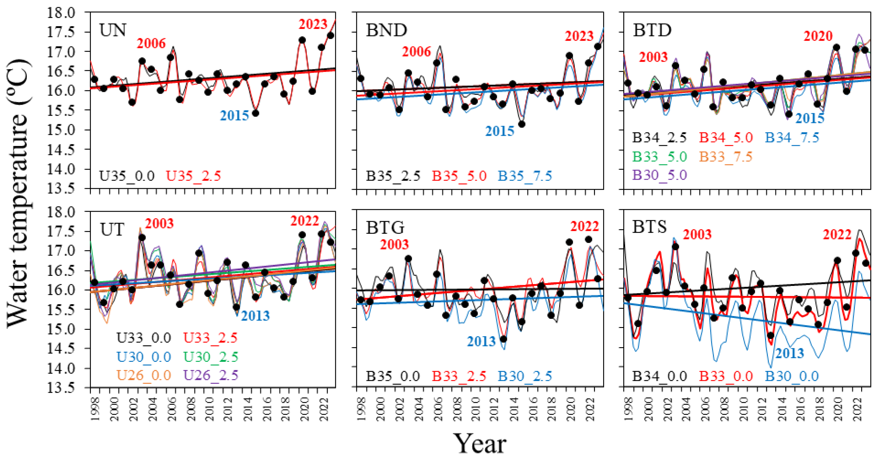
Figure 4.
Cumulative Sum (CuSum) plots of the temperature averaged for each water mass cluster of the estuaries of Bilbao and Urdaibai throughout the study period. Dashed vertical lines split periods with temperature values above (increasing CuSum values), near (similar CuSum values) and below (decreasing CuSum values) the time series mean value in each water mass cluster.
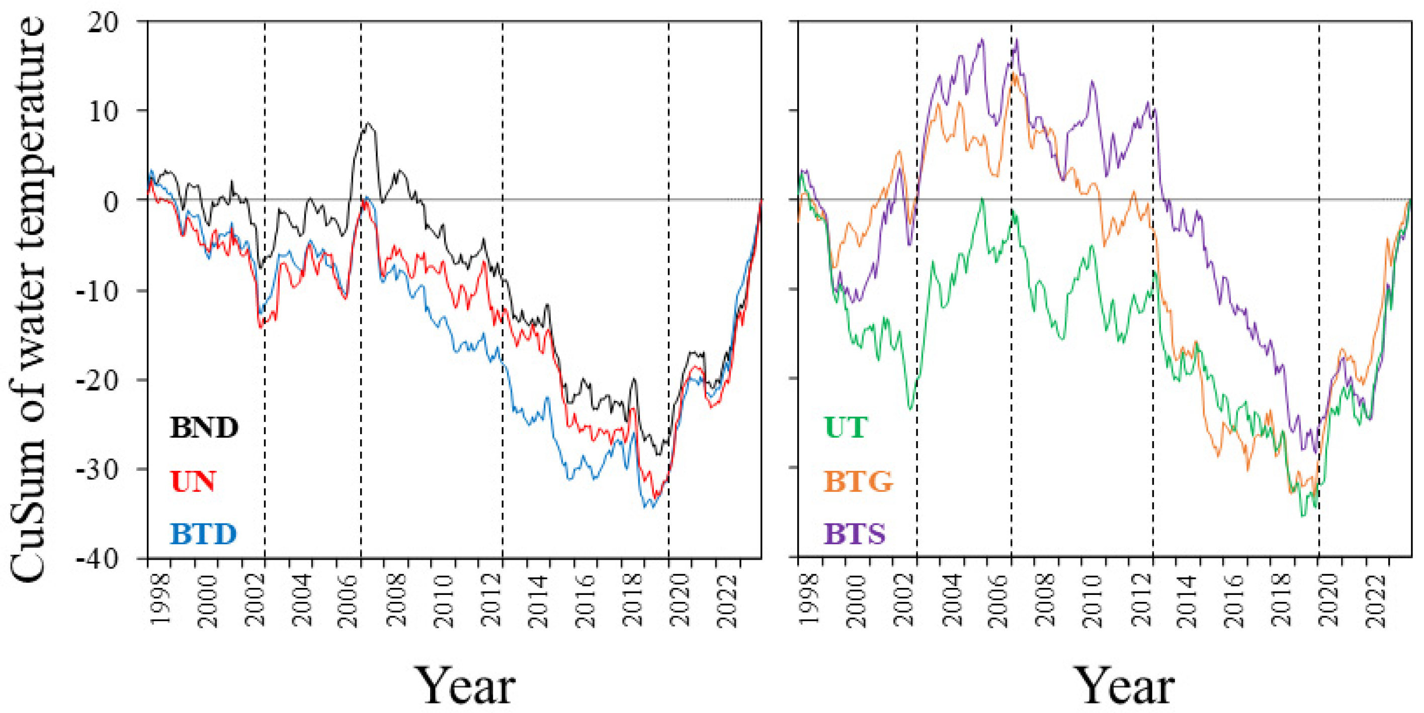
Figure 5.
Year-to-year variations of water temperature values (points) and yearly means (lines), averaged for each water mass cluster of the estuaries of Bilbao and Urdaibai, shown split by season (winter is in blue, spring in green, summer in red, and autumn in brown). Straight lines represent linear fits (regression parameters detailed in Table 2), while dotted lines indicate order 6 polynomial fits.
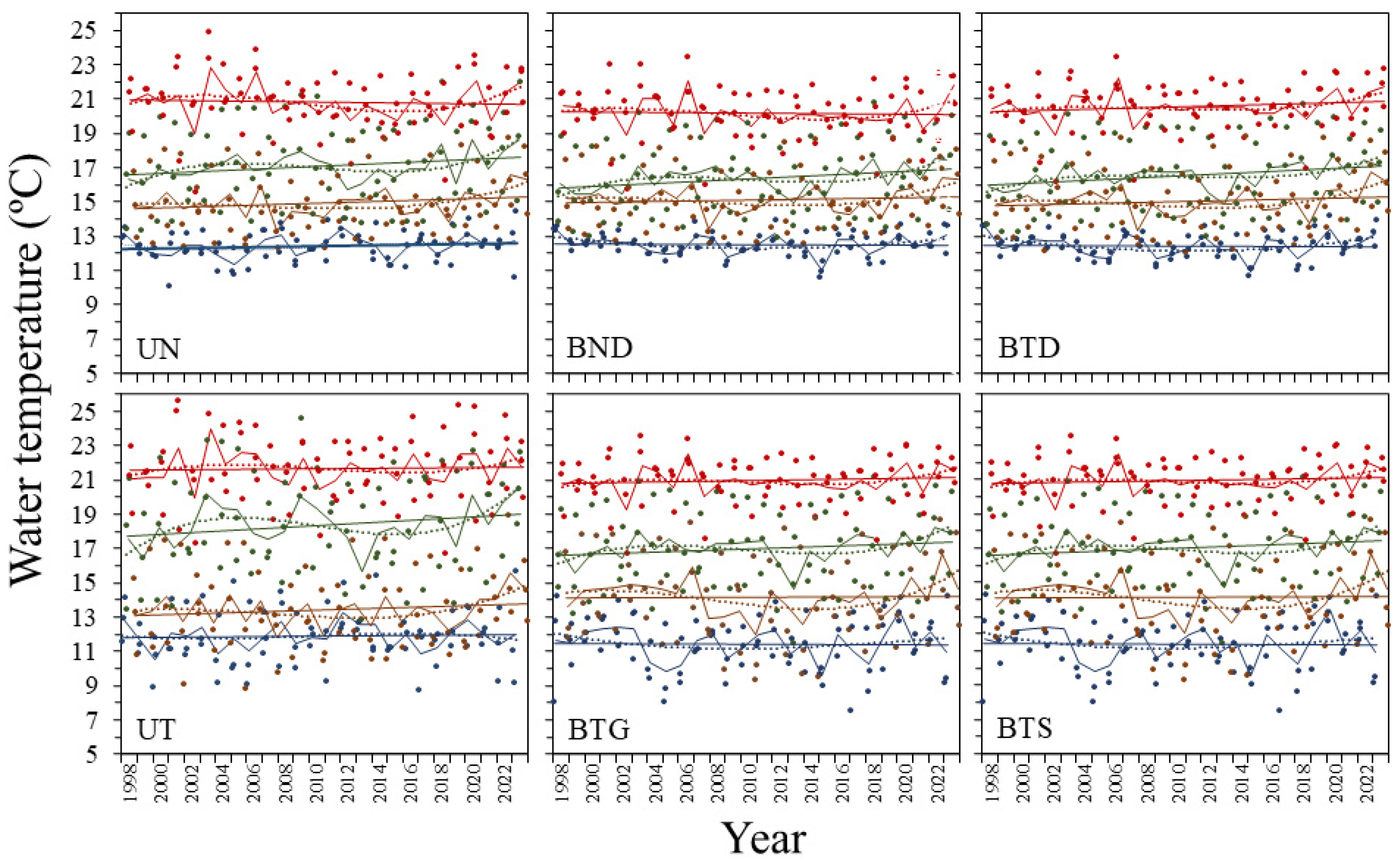
Figure 6.
Monthly water temperature change rates (°C per decade-1) in the water mass clusters of the estuaries of Bilbao and Urdaibai throughout the study period. Winter months are shown in blue, spring months in green, summer months in red, and autumn months in yellow.
Figure 6.
Monthly water temperature change rates (°C per decade-1) in the water mass clusters of the estuaries of Bilbao and Urdaibai throughout the study period. Winter months are shown in blue, spring months in green, summer months in red, and autumn months in yellow.
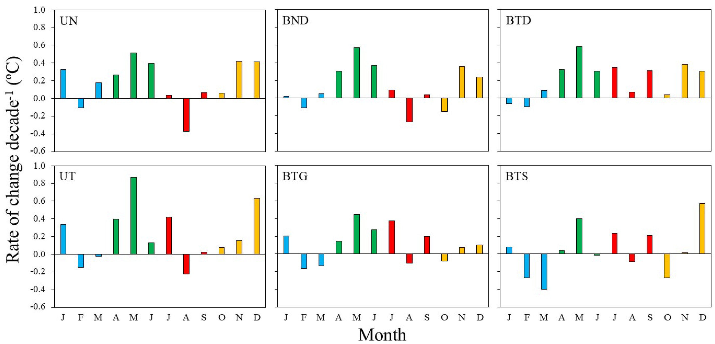
Figure 7.
Monthly variation in the mean water temperature at the analysed sites/depths, clustered into the water masses, of the estuaries of Bilbao and Urdaibai throughout the study period. Estuary, site and depth abbreviations as in Figure 3 caption.
Figure 7.
Monthly variation in the mean water temperature at the analysed sites/depths, clustered into the water masses, of the estuaries of Bilbao and Urdaibai throughout the study period. Estuary, site and depth abbreviations as in Figure 3 caption.
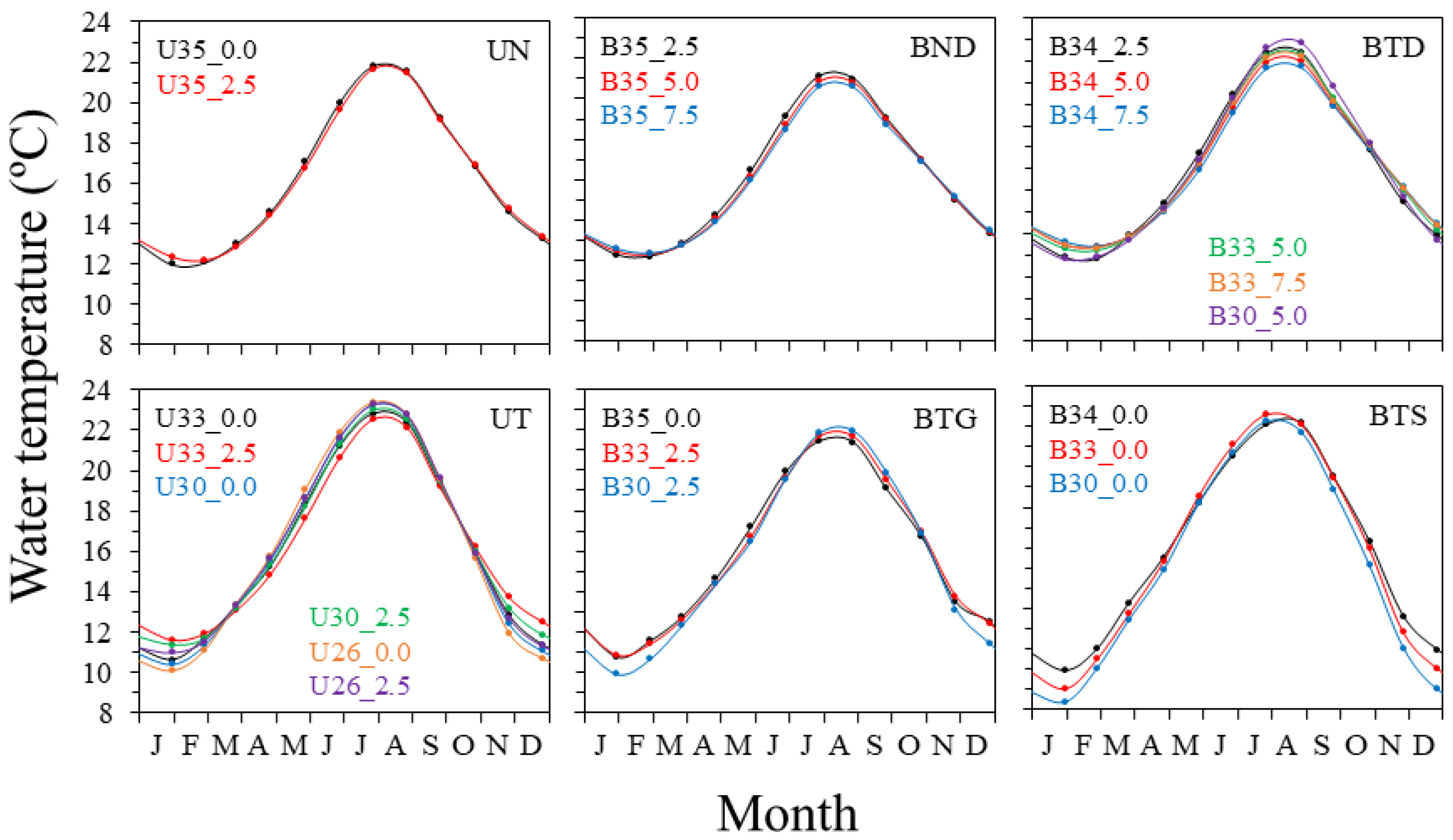
Figure 8.
Month-to-month variation in the mean water temperature averaged for each water mass clusters of the estuaries of Bilbao and Urdaibai for each period identified (see legend for colours) by the CuSum analysis.
Figure 8.
Month-to-month variation in the mean water temperature averaged for each water mass clusters of the estuaries of Bilbao and Urdaibai for each period identified (see legend for colours) by the CuSum analysis.
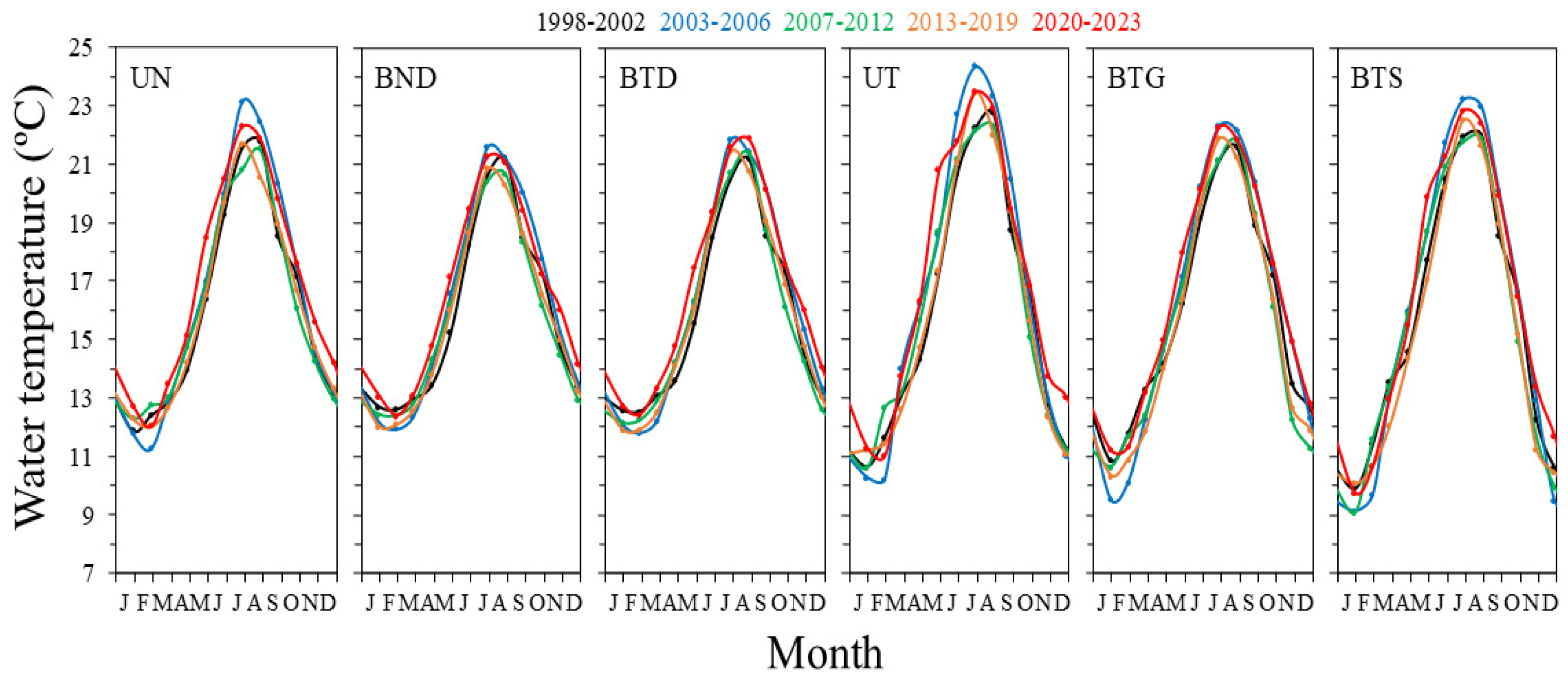
Figure 9.
Variation in the trend component of air temperature (C: Copernicus, S: Sondika, A: Abusu, M: Muxika), river flow (A: Abusu, M: Muxika), upwelling index, and climate teleconnections (NAO index, EA pattern, AMO index, and AO index) throughout the study period. Straight lines represent linear fits (regression parameters detailed in Table 3).
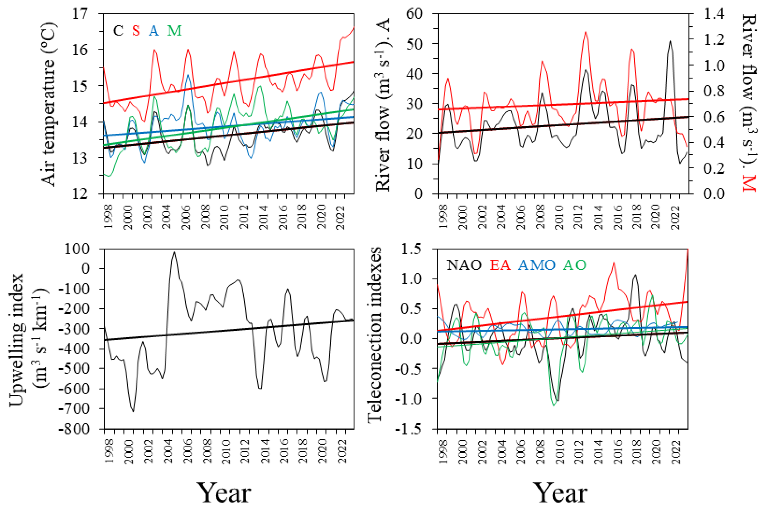
Figure 10.
Monthly rates of change (ºC decade-1) in air temperature (AT), river flow (RF), and upwelling index (UPW) throughout the study period. Winter months are shown in blue, spring months in green, summer months in red, and autumn months in yellow. Data sources include Copernicus (c), Sondika (s), Muxika (m), and Abusu (a).
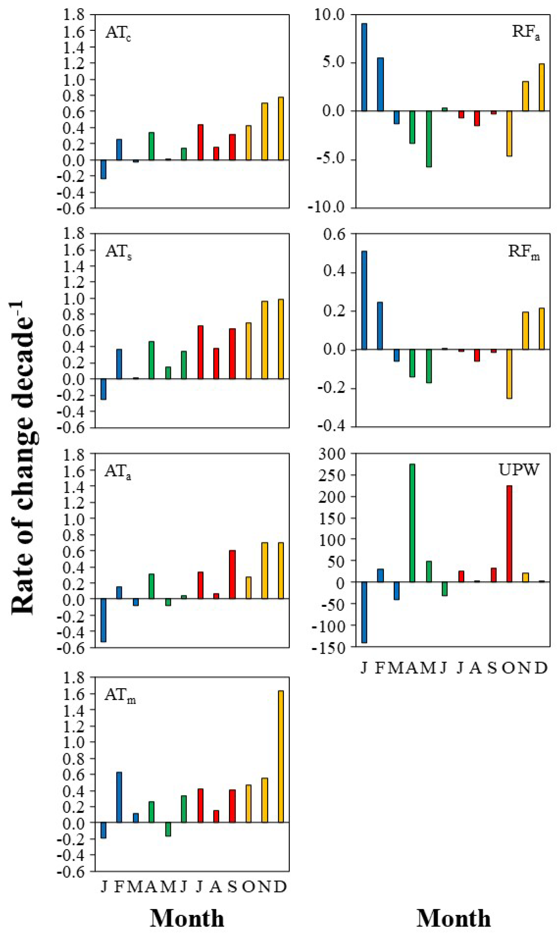

Table 1.
Equation and parameters (R2 and p-value) of the linear regression model describing the variation in the trend component of water temperature at each water cluster over the study period (see Figure 3). Significant p-values in bold. Additionally, the rate of change decade-1 is shown.
Table 1.
Equation and parameters (R2 and p-value) of the linear regression model describing the variation in the trend component of water temperature at each water cluster over the study period (see Figure 3). Significant p-values in bold. Additionally, the rate of change decade-1 is shown.
| Water cluster | Point | Equation | R2 | p-value | Rate of change decade-1 |
|---|---|---|---|---|---|
| UN | U35_0.0 | y = -21.23 + 0.019x | 0.108 | <0.001 | 0.19 |
| U35_2.5 | y = -20.91 + 0.018x | 0.101 | <0.001 | 0.18 | |
| BND | B35_2.5 | y = -3.21 + 0.010x | 0.029 | 0.002 | 0.10 |
| B35_5.0 | y = -9.75 + 0.013x | 0.057 | <0.001 | 0.13 | |
| B35_7.5 | y = -13.98 + 0.015x | 0.074 | <0.001 | 0.15 | |
| BTD | B34_2.5 | y = -20.81 + 0.018x | 0.101 | <0.001 | 0.18 |
| B34_5.0 | y = -20.83 + 0.018x | 0.107 | <0.001 | 0.18 | |
| B34_7.5 | y = -22.39 + 0.019x | 0.114 | <0.001 | 0.19 | |
| B33_5.0 | y = -32.13 + 0.024x | 0.202 | <0.001 | 0.24 | |
| B33_7.5 | y = -32.55 + 0.024x | 0.217 | <0.001 | 0.24 | |
| B30_5.0 | y = -24.89 + 0.020x | 0.121 | <0.001 | 0.20 | |
| UT | U33_0.0 | y = -30.52 + 0.023x | 0.136 | <0.001 | 0.23 |
| U33_2.5 | y = -25.29 + 0.021x | 0.101 | <0.001 | 0.21 | |
| U30_0.0 | y = -12.66 + 0.014x | 0.047 | <0.001 | 0.14 | |
| U30_2.5 | y = -19.72 + 0.018x | 0.073 | <0.001 | 0.18 | |
| U26_0.0 | y = -33.82 + 0.025x | 0.125 | <0.001 | 0.25 | |
| U26_2.5 | y = -33.87 + 0.025x | 0.135 | <0.001 | 0.25 | |
| BTG | B35_0.0 | y = 11.60 + 0.002x | 0.001 | 0.570 | 0.02 |
| B33_2.5 | y = -23.49 + 0.020x | 0.107 | <0.001 | 0.20 | |
| B30_2.5 | y = -1.06 + 0.008x | 0.017 | 0.022 | 0.08 | |
| BTS | B34_0.0 | y = -13.95 + 0.015x | 0.042 | <0.001 | 0.15 |
| B33_0.0 | y = 18.95 - 0.002x | 0.0004 | 0.740 | -0.02 | |
| B30_0.0 | y = 75.66 - 0.030x | 0.096 | <0.001 | -0.30 |
Table 2.
Rate of temperature change decade-1 for each water mass cluster in each season over the study period (see Figure 5).
Table 2.
Rate of temperature change decade-1 for each water mass cluster in each season over the study period (see Figure 5).
| Rate of change decade-1 | ||||
|---|---|---|---|---|
| Water cluster | Winter | Spring | Summer | Autumn |
| UN | 0.14 | 0.42 | -0.10 | 0.28 |
| BND | -0.01 | 0.44 | -0.05 | 0.13 |
| BTD | -0.02 | 0.43 | 0.23 | 0.22 |
| UT | 0.07 | 0.49 | 0.05 | 0.27 |
| BTG | -0.02 | 0.31 | 0.14 | 0.01 |
| BTS | -0.18 | 0.17 | 0.10 | 0.08 |
Table 3.
Equation and parameters (R2 and p-value) of the linear regression model describing the variation in the trend component of air temperature (from various sources), river flow, upwelling index, and teleconnection indices (NAO, EA, AMO, AO) over the study period (see Figure 9). Significant p-values in bold. The rate of change decade-1 is also shown.
| Variable | Type | Equation | R2 | p-value | Rate of change decade-1 |
|---|---|---|---|---|---|
| Air temperature | Copernicus | y = -41.03 + 0.027x | 0.218 | <0.001 | 0.27 |
| Sondika | y = -73.63 + 0.044x | 0.339 | <0.001 | 0.44 | |
| Abusu | y = -26.16 + 0.020x | 0.102 | <0.001 | 0.20 | |
| Muxika | y = -63.62 + 0.039x | 0.278 | <0.001 | 0.39 | |
| River flow | Abusu | y = -396.62 + 0.209x | 0.038 | 0.001 | 0.21 |
| Muxika | y = -5.53 + 0.003x | 0.016 | 0.024 | 0.03 | |
| Upwelling index | y = -7985.5 + 3.805x | 0.027 | 0.004 | 38.05 | |
| Teleconnection indices | NAO | y = -14.32 + 0.007x | 0.022 | 0.008 | 0.07 |
| EA | y = -38.19 + 0.019x | 0.159 | <0.001 | 0.19 | |
| AMO | y = -5.47 + 0.003x | 0.047 | <0.001 | 0.03 | |
| AO | y = -24.88 + 0.002x | 0.081 | <0.001 | 0.02 |
Table 4.
Spearman’s rank correlation coefficients between water temperature and local factors (AT: air temperature, RF: river flow, UPW: upwelling index) and climate teleconnections (NAO: North Atlantic Oscillation index, EA: East Atlantic index, AMO: Atlantic Multidecadal Oscillation index, AO: Arctic Oscillation index), analysed by season at each water mass cluster. Only statistically significant correlations (p < 0.05) are shown. Correlations with p < 0.001 are highlighted in bold. Shaded cells indicate the highest correlation for each identified water mass cluster and season. Data sources of local factors include Copernicus (c), Sondika (s), Abusu (a), and Muxika (m).
| Local factors | Teleconnections | |||||||||
|---|---|---|---|---|---|---|---|---|---|---|
| Water cluster | Season | ATc | ATs | ATa/m | RFa/m | UPW | NAO | EA | AMO | AO |
| UN | Winter | 0.589 | 0.602 | 0.494 | -0.306 | 0.241 | ||||
| Spring | 0.907 | 0.881 | 0.868 | -0.537 | 0.430 | 0.261 | ||||
| Summer | 0.593 | 0.514 | 0.521 | |||||||
| Autumn | 0.871 | 0.861 | 0.780 | -0.483 | -0.356 | 0.335 | ||||
| BND | Winter | 0.496 | 0.473 | 0.410 | -0.418 | 0.291 | ||||
| Spring | 0.893 | 0.874 | 0.882 | -0.442 | 0.398 | 0.344 | ||||
| Summer | 0.559 | 0.503 | 0.551 | 0.240 | ||||||
| Autumn | 0.844 | 0.835 | 0.805 | -0.466 | -0.331 | 0.294 | ||||
| BTD | Winter | 0.599 | 0.537 | 0.536 | -0.434 | 0.304 | 0.233 | |||
| Spring | 0.918 | 0.893 | 0.897 | -0.525 | 0.411 | 0.314 | ||||
| Summer | 0.645 | 0.609 | 0.647 | 0.233 | ||||||
| Autumn | 0.868 | 0.858 | 0.833 | -0.509 | -0.331 | 0.326 | ||||
| UT | Winter | 0.681 | 0.700 | 0.632 | 0.261 | |||||
| Spring | 0.896 | 0.886 | 0.864 | -0.607 | 0.476 | 0.274 | ||||
| Summer | 0.608 | 0.525 | 0.624 | 0.313 | ||||||
| Autumn | 0.835 | 0.839 | 0.811 | -0.526 | -0.420 | 0.319 | ||||
| BTG | Winter | 0.667 | 0.650 | 0.624 | -0.486 | 0.259 | 0.244 | |||
| Spring | 0.925 | 0.904 | 0.907 | -0.504 | 0.448 | 0.331 | ||||
| Summer | 0.679 | 0.624 | 0.701 | -0.273 | ||||||
| Autumn | 0.836 | 0.812 | 0.812 | -0.669 | 0.241 | -0.322 | 0.332 | |||
| BTS | Winter | 0.737 | 0.737 | 0.722 | -0.267 | 0.317 | ||||
| Spring | 0.855 | 0.843 | 0.854 | -0.491 | 0.481 | 0.263 | ||||
| Summer | 0.633 | 0.552 | 0.678 | -0.319 | 0.298 | |||||
| Autumn | 0.878 | 0.853 | 0.866 | -0.624 | -0.384 | 0.331 | ||||
Disclaimer/Publisher’s Note: The statements, opinions and data contained in all publications are solely those of the individual author(s) and contributor(s) and not of MDPI and/or the editor(s). MDPI and/or the editor(s) disclaim responsibility for any injury to people or property resulting from any ideas, methods, instructions or products referred to in the content. |
© 2025 by the authors. Licensee MDPI, Basel, Switzerland. This article is an open access article distributed under the terms and conditions of the Creative Commons Attribution (CC BY) license (https://creativecommons.org/licenses/by/4.0/).
Copyright: This open access article is published under a Creative Commons CC BY 4.0 license, which permit the free download, distribution, and reuse, provided that the author and preprint are cited in any reuse.


