Submitted:
28 July 2025
Posted:
29 July 2025
Read the latest preprint version here
Abstract
This study investigated the vertical structure of an anticyclonic eddy (AE) in the northern South China Sea (SCS) in August 2017 and its response to Typhoon Hato using underwater glider data and satellite altimeter data. Additionally, comparative experiments with and without typhoon forcing were conducted using the Regional Ocean Modeling System (ROMS) for supplementary analysis. The observational results reveal that the maximum temperature and salinity differences between the center and edge of the upper layer of the AE did not occur at the sea surface but near the 100 m depth, with a maximum temperature difference of 2.86°C and a maximum salinity difference of 0.65 PSU. The typhoon caused a significant temperature decrease above 200 m, with the maximum cooling (~2°C) occurring near 50 m. Near this depth, salinity initially increased due to upwelling but later decreased due to surface mixing. The most pronounced cooling and salinity changes occurred one day after the typhoon passage, followed by a gradual deepening of the mixed layer over the next four days, with conditions below the mixed layer largely returning to pre-typhoon states. The numerical simulations indicate that upwelling rapidly intensified during the typhoon’s passage, consistent with the observational temperature changes in the upper ocean. The typhoon’s wind stress increased kinetic energy at the AE site, while the input of positive vorticity reduced absolute vorticity, disrupting the surface anticyclonic flow structure. One day after the typhoon, the flow field gradually recovered.
Keywords:
anticyclonic eddy
; typhoon
; underwater glider
; northern South China Sea
1. Introduction
Mesoscale eddy is transient yet intense mesoscale oceanic phenomena, accounting for the majority of kinetic energy in the ocean. They exhibit strong nonlinearity[1] and play a significant role in the global transport and redistribution of oceanic mass and energy[2], thereby influencing atmospheric responses[3], climate variability, and interactions with other oceanic processes. The South China Sea (SCS), the largest and deepest semi-enclosed marginal sea in the western Pacific, is a region with frequent and abundant mesoscale eddy activity[4], connected to the open ocean and adjacent seas through multiple straits[5].
Previous studies have extensively investigated the characteristics of mesoscale eddies in the SCS, such as their spatial distribution, radius, amplitude, and other properties, using eddy detection methods based on flow fields and sea surface height data[6]. However, since satellite altimeters can only capture surface information, analyzing the three-dimensional structure of mesoscale eddies relies on in-situ observations or numerical modeling. Underwater glider, a novel type of autonomous oceanographic instrument, is buoyancy-driven and capable of following preprogrammed paths while equipped with various sensors to collect temperature, conductivity, sound velocity, and other hydrographic data[7]. They offer advantages such as extensive spatial coverage, long endurance, and high resolution. Currently, underwater gliders have been widely employed in observing mesoscale eddies and analyzing their three-dimensional structures. For instance, Qiu et al.[8] tracked an anticyclonic eddy (AE) in the northern SCS using three gliders, revealing a lifespan of two months and an average radius of 70 km. Their study found that background currents induced asymmetries in the eddy’s shape, velocity, and heat distribution. Shu et al.[9] combined glider and CTD data to investigate an AE in the SCS in 2017, demonstrating that its three-dimensional structure was strongly influenced by sloping topography. Qiu et al.[10] observed an AE in the northern SCS from April to June 2018 using gliders, identifying submesoscale frontal structures ahead of the eddy and using numerical modeling to show that baroclinic processes dominated its deformation. Additionally, Li et al.[11] designed a coordinated glider observation network to reconstruct the 3D structure of an AE in the northern SCS, analyzing its thermohaline characteristics and suggesting its possible generation through Kuroshio shedding.
The northern SCS is also a region frequently traversed by typhoons. Typhoon specifically refers to a tropical cyclone (TC) generated in the northwest Pacific Ocean, is an intense low-pressure weather system characterized by strong winds, heavy rainfall, and low atmospheric pressure, often causing significant destruction. Its powerful cyclonic wind field injects positive vorticity into the ocean while enhancing upper-ocean mixing[12]. The intense disturbance induced by typhoons in the upper ocean can substantially influence the generation and evolution of mesoscale eddies, altering their shape, intensity, lifespan, and other properties, with the extent of impact depending on the typhoon’s path and strength[13]. The effects of typhoons on mesoscale eddies vary depending on the eddy’s nature[14]. Huang et al.[15] investigated the impact of a typhoon on a dipole eddy pair and found that the typhoon caused asymmetry in the dipole structure. After the typhoon’s passage, internal interactions within the dipole eddy led to faster stabilization compared to an isolated eddy. When a typhoon interacts with a cyclonic eddy, the eddy tends to intensify[16]. Post-typhoon, the cyclonic eddy exhibits increased amplitude and rotational speed, resulting in enhanced kinetic energy, an expanded radius, and altered shape[17]. Vertically, the combined upwelling induced by both the cyclonic eddy and the typhoon strengthens surface cooling and enhances vertical material transport[18]. In contrast, the influence of typhoons on AEs is generally opposite to that on cyclonic eddies. The changes in upper-ocean currents and density structure induced by typhoons can weaken or even dissipate AEs[19]. The warm-core anomaly of AEs may intensify passing typhoons, while typhoon-induced upwelling counteracts the eddy’s downward flow, leading to a slight temperature reduction near the eddy. However, stronger AEs can retain their structure, establishing a negative feedback mechanism between the eddy and the typhoon[20]. In terms of amplitude, absolute vorticity, and radius, AEs generally exhibit weakening trends, accompanied by significant losses in heat[21] and kinetic energy.
This study primarily employs observational data and numerical modeling to analyze the three-dimensional structural characteristics of an AE generated near the Luzon Strait in June 2017 and its variations under typhoon influence. Section 1 investigates the evolution process and fundamental characteristics of the AE based on satellite altimeter data. Section 2 utilizes underwater glider observations to analyze the vertical thermohaline structure of the eddy and its response process to Typhoon Hato. Section 3 conducts a comparative analysis of the eddy's response under typhoon and non-typhoon conditions using the Regional Ocean Modeling System (ROMS).
2. Materials and Methods
2.1. Underwater Glider Data
In August 2017, Tianjin University of China deployed 12 "Petrel II" underwater gliders in the northern SCS. Each glider was equipped with a CTD sensor to measure temperature, pressure, and salinity[11,22]. The gliders operated from August 4 to 29, 2017, with their trajectories shown in Figure 1. The average horizontal sampling resolution was approximately 2.25 km, and the mean horizontal speed was about 1.68 km/h. The vertical sampling range spanned from 15.05 m to 980.55 m, with an average vertical resolution of 0.8 m and a mean vertical velocity of approximately 0.2 m/s[11,22]. The operational periods and maximum diving depths varied among the gliders. Since the collected data were non-gridded in both time and space, preprocessing was required. During each dive or climb, a glider typically covered an average horizontal displacement of about 2.3 km. To ensure data density, measurements from both descending and ascending profiles were utilized. The raw data were interpolated onto a standardized vertical grid with 0.2 m intervals.
2.2. Satellite Altimeter Data
The study utilized the global gridded satellite altimeter reprocessed dataset from the Copernicus Marine Environment Monitoring Service (CMEMS), which includes sea surface height anomaly (SSHA), absolute dynamic topography (ADT), geostrophic velocity, and geostrophic velocity anomaly. These anomalies were calculated relative to the 20-year mean (1993-2012). The data were obtained by merging multiple satellite altimeters and applying Optimal Interpolation, yielding a horizontal spatial resolution of 0.125° and a temporal resolution of 1 day. These data were used to identify and track mesoscale eddies in this study.
2.3. Typhoon Information
Typhoon data were obtained from the International Best Track Archive for Climate Stewardship (IBTrACS), which consolidates best-track data from multiple global Tropical Cyclone Warning Centers (TCWCs) and Regional Specialized Meteorological Centers (RSMCs) designated by the World Meteorological Organization. This study specifically used data provided by U.S. agencies (National Hurricane Center [NHC], Joint Typhoon Warning Center [JTWC], and Central Pacific Hurricane Center [CPHC]). For Typhoon Hato, which passed through the northern SCS in August 2017, the dataset provided 3-hourly information including the typhoon's center position, central pressure, and radius of maximum wind speed.
2.4. Mesoscale Eddy Identification Method
This study adopts the winding angle (WA) algorithm for eddy detection and tracking, a streamline geometry-based method for identifying mesoscale eddies[6,23]. The algorithm begins by scanning 4×4 grid windows across the study domain to locate local extrema in SSHA as potential eddy cores. From each candidate core, the method examines surrounding streamlines by expanding outward radially, confirming an eddy when the accumulated turning angle of examined streamlines reaches 2π radians. The eddy boundary is then defined as the outermost closed streamline that encompasses only the target extremum. To track eddies through time and depth, we implement a conservative approach that considers eddies detected within a 30 km radius (based on the typical 30 km/day translation speed of SCS eddies[24]) as the same feature. Several key eddy properties are quantified in this study:
The eddy radius(R) is calculated as the equivalent circular radius of the eddy area with a minimum threshold of 30 km:
where S represents the area enclosed by the eddy's boundary streamline.
The amplitude(A) represents the mean SSHA difference between the eddy center and its boundary:
where denotes the sea surface height anomaly at the eddy core and represents the SSHA along the boundary streamline.
The eddy kinetic energy(EKE) and vorticity(ζ) are derived from the geostrophic velocity fields within the eddy structure:
where x and y indicate longitudinal and latitudinal directions respectively.
2.5. Numerical Model Configuration
To complement the glider observations which lack current measurements, we conducted two parallel numerical experiments with different wind forcing scenarios using the ROMS (version 3.9)[25]. The model domain covers the SCS with a horizontal resolution of 1/12° (~9 km at the equator) and employs a terrain-following S-coordinate system with 30 vertical layers to better resolve coastal and subsurface processes. The turbulence closure scheme is a Generic Mixed Length-Scale (GLS) turbulence closure scheme. Initial and boundary conditions were derived from the daily Mercator Ocean global analysis product, while atmospheric forcing was provided by the 6-hourly ERA5 reanalysis dataset. The simulation period spans August 2017, initialized at 00:00 UTC on August 1st to capture the complete evolution of the target eddy system. A control run with baseline climatological forcing was compared against a perturbed run incorporating additional wind stress derived from IBTrACS data, allowing for isolation of typhoon-induced perturbations from background variability. This configuration follows established practices for South China Sea eddy simulations, with particular attention to resolving mesoscale processes through appropriate horizontal resolution and vertical layer distribution.
3. Results and Discussion
3.1. Evolution analysis of the AE in the Northern SCS Based on Satellite Altimeter Data
From June to September 2017, daily SSHA and surface geostrophic velocity data were obtained from the CMEMS global gridded satellite altimeter reprocessed dataset. The WA detection algorithm was applied to identify the position and boundaries of an AE located southwest of Taiwan in the northern SCS.
The AE persisted from June 25 to September 10, 2017. It initially formed as a closed anticyclonic circulation in the Luzon Strait on June 25 before propagating westward (Figure 2). On July 27, the eddy altered its trajectory to a southwestward direction. Between August 4 and 29, a fleet of "Petrel II" underwater gliders deployed by Tianjin University conducted continuous monitoring of the eddy, collecting high-resolution temperature, salinity and pressure data (Figure 3 displays the daily operational glider numbers and their positions). The eddy subsequently turned southward on August 29 before eventually dissipating after September 10.
The AE exhibited rapid growth in radius, amplitude, and kinetic energy following its formation (Figure 4), reaching peak intensity on July 25 before undergoing three significant typhoon interactions. After Typhoon Haitang's passage on July 29, the eddy's radius, amplitude, and kinetic energy decreased sharply, with the radius recovering after August 3 while amplitude and kinetic energy stabilized at reduced levels. Subsequent passages of Typhoons Hato (August 22) and Pakhar (August 26) caused further rapid declines in all parameters, followed by gradual recovery after August 31 and persistent weakening leading to dissipation after September 3. Throughout its lifespan, the eddy maintained mean values of 93.9 km radius, 10.6 cm amplitude, 0.042 m²/s² kinetic energy, -7.2×10⁻⁶ rad/s vorticity, and 7.94 km/day translation speed, demonstrating characteristic responses to multiple typhoon forcings while preserving its core structure through recovery periods.
3.2. Vertical Thermohaline analysis of Mesoscale Eddy Based on Underwater Glider Observations
In the Northern Hemisphere, AEs induce seawater convergence toward their cores, transporting warmer surface waters downward and resulting in positive temperature anomalies within the eddy center relative to its periphery. This thermal signature serves as a reliable indicator for identifying AE positions.
The trajectories of the 12 underwater gliders predominantly followed straight-line paths (Figure 1). To characterize the spatial distribution of temperature and salinity across the surveyed area, all glider data were integrated and horizontally interpolated onto several depth layers (Figure 5). The analysis revealed a distinct warm-core feature between 30-150m depths northwest of 20.5°N and 118.5°E, which was confirmed as the AE center through comparison with the eddy position in Figure 3. Below 200m, this region maintained warmer characteristics but without a clearly defined core. While surface temperature variations were modest (<1°C), substantial thermal contrasts (>2°C) between maximum and minimum temperatures were observed between 75-200m depths, indicating maximum eddy strength in this subsurface layer rather than at the surface.
The salinity distributions (Figure 5b) exhibited analogous patterns, with a pronounced high-salinity core in the same geographic region that became less distinct below 200m while retaining elevated salinity characteristics. From the surface to 100m, salinity increased with depth, exceeding 34.9 PSU at maximum values. Below this depth, salinity decreased gradually, maintaining values above 34.7 PSU between 75-150m depths. Notably, the salinity difference between 75m and 100m exceeded 0.2 PSU, demonstrating strong vertical haline stratification within the eddy's core region. These thermohaline structures collectively illustrate the three-dimensional signature of the AE, with maximum intensity manifested in subsurface layers rather than at the surface.
Figure 6.
Locations of underwater gliders in relation to the anticyclonic eddy on 5 August 2017. Background fields display the SSHA and geostrophic currents, with the red contour marking the eddy boundary identified by the WA method.
Figure 6.
Locations of underwater gliders in relation to the anticyclonic eddy on 5 August 2017. Background fields display the SSHA and geostrophic currents, with the red contour marking the eddy boundary identified by the WA method.
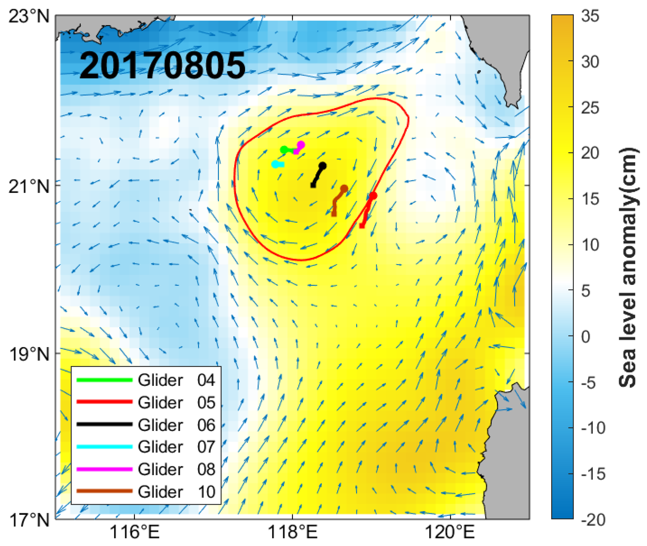
The underwater gliders were strategically deployed at different locations within the eddy to enable comparative analysis of temperature and salinity distributions across various eddy regions. Among them, Gliders 05, 06, and 10 exhibited the longest and nearly parallel trajectories (Figure 1). Analysis of daily relative positions between the eddy and gliders revealed that on August 5, Glider 06 was positioned closest to the eddy center, while Glider 05 was located precisely at the eddy boundary, with Glider 10 situated midway between them. The precise distances from these gliders to the eddy center are provided in Table 1.
The temperature and salinity profiles collected by the three underwater gliders are presented in Figure 7. Comparative analysis of their temperature profiles (Figure 7a) reveals distinct isotherm depressions in Gliders 06 and 10 within the eddy interior - a characteristic signature of AEs resulting from convergent surface water transport downward[26]. The salinity profiles (Figure 7b) exhibit a pronounced high-salinity water mass (>34.7 PSU) between 100-200 m depths. This saline core demonstrates clear radial attenuation, with its vertical thickness progressively decreasing as the gliders move away from the eddy center, eventually disappearing beyond the eddy boundary. These observations capture the three-dimensional thermohaline structure of the AE, confirming its subsurface-intensified nature.
Although the anticyclonic flow field drives downward transport of warm surface waters, turbulent mixing in the ocean surface layer weakens the warm-core signature near the surface. For Glider 06 (near the eddy center), the maximum temperature difference relative to Glider 05 (near the boundary) reached 2.86°C at 122 m depth, while the maximum salinity difference was 0.65 PSU at 61 m depth (Table 2). In contrast, Glider 10 (between the center and boundary) exhibited a smaller maximum temperature difference of 1.67°C at 94 m depth and a salinity difference of 0.14 PSU at 61 m depth compared to Glider 05. These observations highlight that horizontal distance from the eddy center is the dominant factor controlling temperature distribution within the eddy, with the strongest anomalies occurring in the subsurface layer (50–200 m) rather than at the surface.
The temperature and salinity differences decreased rapidly from their maximum anomaly depths down to approximately 300 m (Figure 8b, d), with the disparities between Glider 06 and Glider 10 showing similar attenuation trends. Below 300 m, the residual thermohaline anomalies became substantially weaker (Table 3), with Glider 06 recording maximum differences of only 0.85°C at 358 m and 0.09 PSU at 350 m, while Glider 10 exhibited even smaller anomalies of 0.72°C at 361 m and 0.07 PSU at 347 m. These markedly reduced gradients below 300 m depth clearly demonstrate the rapidly diminishing influence of the AE in deeper layers, reflecting its primarily upper-ocean character.
3.3. Vertical Structural Changes of the Mesoscale Eddy Under Typhoon Influence
All times mentioned in this section are in Coordinated Universal Time (UTC).
3.3.1 Typhoon-Induced Thermohaline Variations Revealed by Underwater Gliders
Typhoon Hato originated over the western North Pacific and intensified into a tropical storm by 06:00 on August 21 (Figure 9). Tracking westward, it crossed the Luzon Strait at 00:00 on August 22, attaining severe tropical storm status. The system then took a northwestward trajectory, arriving over the AE at 06:00. It further intensified to typhoon strength by 09:00 during its 6-hour passage above the eddy, before departing the eddy region after 12:00. Hato reached severe typhoon intensity by 21:00 and made landfall in Guangdong Province, China at 06:00 on August 23, eventually dissipating as a tropical depression by 12:00 on August 24, the typhoon maintained an average translation speed of 24.2 km/h.
During Typhoon Hato's passage, four underwater Gliders 06, 09, 12, and 13 were operational (Figure 9). Notably, all gliders except Glider 13 (located outside the AE) were positioned within the eddy's boundary. As Glider 12 ceased operation after 22 August, our subsequent analysis focuses primarily on data from Gliders 6 and 9 to examine the typhoon's impact on the thermohaline structure within the eddy.
During Typhoon Hato's passage over the AE on 22 August, Glider 06 recorded significant cooling across nearly all depth layers (22–24 August), manifested by upward displacement of isotherms in Figure 10a. The 30°C isotherm shoaled from ~40 m to <15 m, indicating strong wind-driven mixing and upwelling. Post-24 August, downward migration of isotherms marked the beginning of thermal recovery. Glider 09, positioned west of Glider 06, exhibited similar but delayed responses due to its offset location relative to the typhoon track.
Salinity changes were more complex (Figure 10b). Above 125 m, isohalines mirrored thermal patterns (upward shift), with salinity increasing from the surface to 125 m before decreasing with depth. On 22–23 August, salinity rose above 125 m but declined below this depth. By 24 August, while upper-layer salinity began recovering, ongoing isohaline uplift below 125 m compressed the high-salinity core (>34.7 PSU).
To investigate the typhoon's impact on the eddy during and after its passage, we conducted a comparative analysis of temperature and salinity changes on 22 August (during typhoon passage) versus 23, 25, and 27 August (post-typhoon period). However, the continuous movement of underwater gliders introduced significant variability in observations between the eddy center and periphery. To isolate the typhoon's influence from positional effects, we implemented the following normalization procedures:
For Glider 06, which operated continuously throughout the observational period, we calculated its daily distance from the eddy center alongside the eddy's radius (Figure 11a). To account for the eddy's size variability, we normalized the glider-eddy center distance by the daily radius (Figure 11b), treating the eddy as a circular feature. This normalization revealed that Glider 06 occupied similar relative positions on the following dates: 22 August (typhoon passage) vs. 17 August (pre-typhoon baseline); 23 & 25 August (recovery phase) vs. 16 August (pre-typhoon baseline); 27 August (late recovery) vs. 18 August (pre-typhoon baseline). Using these matched pairs, we analyzed vertical thermohaline profiles and their anomalies (Figure 12):
Typhoon-induced perturbations extended to approximately 300 m depth (Figure 12). As the typhoon passed, the temperature within the eddy gradually decreased (Figure 12b). By 23 August, when the typhoon had completely passed, the upper layer reached its lowest average temperature, with the maximum cooling (~2°C) occurring near 50 m depth. This resulted from typhoon-driven upwelling surpassing the AE's inherent downwelling, causing the upward transport of colder subsurface water. Subsequently, the upper-layer temperature began to recover, though cooling persisted above 30 m due to strong wind-driven mixing. By 27 August, the subsurface layer had largely returned to pre-typhoon conditions, but the combined cooling above 50 m and warming below 50 m led to a deepening of the mixed layer beyond 50 m, accompanied by a notable drop in the layer's mean temperature.
Concurrently, the surface salinity within the eddy gradually increased (Figure 12c), while subsurface salinity decreased, albeit with a much smaller magnitude compared to the surface salinification. On 23 August, when the typhoon had fully passed, surface salinity peaked, with the maximum increase exceeding 0.25 PSU near 50 m (Figure 12d), again due to the vertical transport of saltier subsurface water. Subsequently, salinity continued to rise above 50 m while decreasing rapidly between 50–100 m (maximum reduction >0.3 PSU). The post-typhoon salinity evolution (25–27 August) indicated intense mixing in the surface layer, whereas changes at 150–300 m were minor and gradually reverted toward pre-typhoon conditions.
3.3.2. Numerical Experiment Design and Result Validation
To compare the different impacts on the AE under typhoon and non-typhoon conditions, we conducted numerical experiments by replacing the original typhoon wind field with a designed typhoon-free wind field during the period before and after the typhoon approached the mesoscale eddy (21–24 August; Figure 13a).
To isolate the typhoon’s impact while preserving the ambient wind field, the typhoon-free wind field (V) was constructed using a superposition method[27], formulated as:
Where represents the averaged wind in the SCS on that day, is the original typhoon-containing wind field, and denotes a Gaussian weighting function with r is the distance from the typhoon center, and R is the radius of 34-kt winds (90–150 km during the typhoon period). Beyond r > 370 km, (r) < 0.05, meaning the wind field reverts to the original ERA5 data.
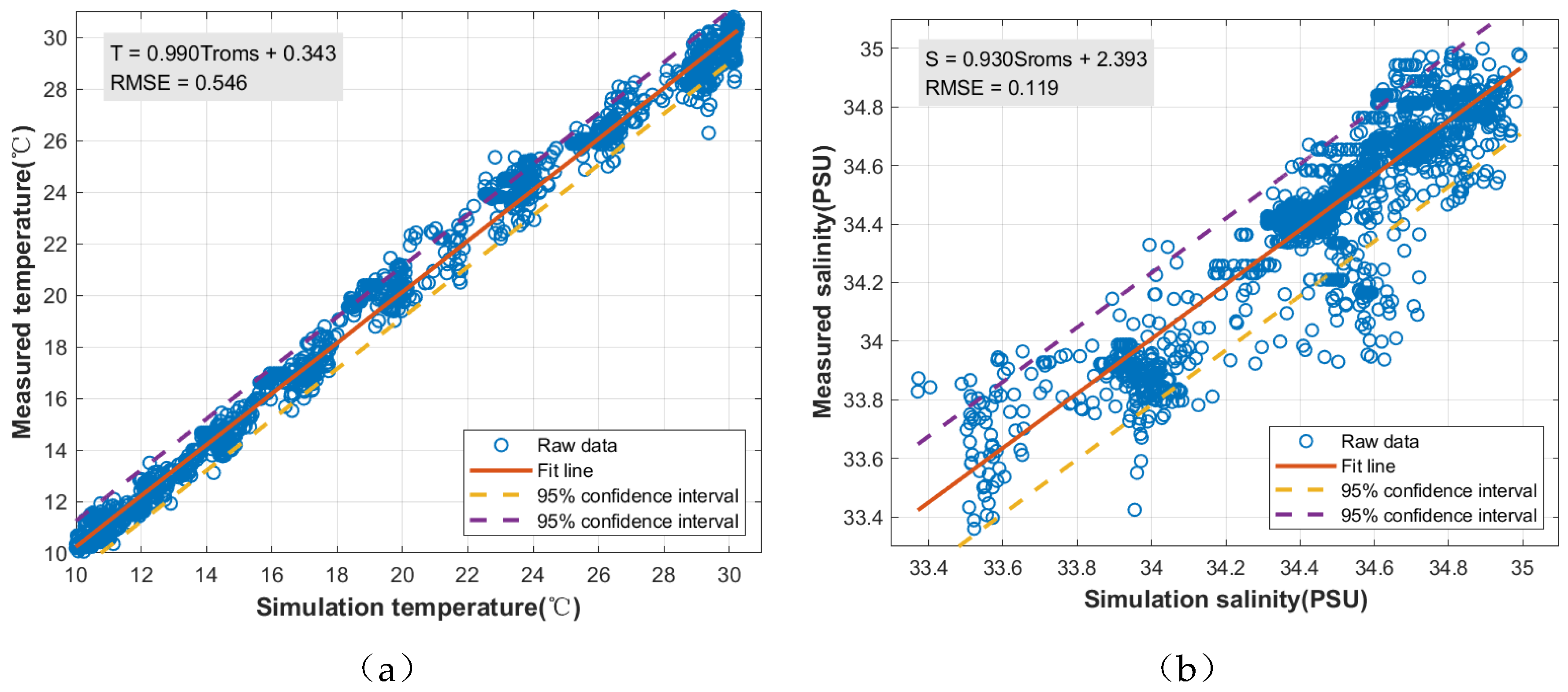
The ROMS simulation outputs were validated against underwater glider observations through spatiotemporal interpolation and statistical analysis. For temperature fields, the model demonstrated exceptional agreement with glider data, yielding a correlation coefficient of 0.990 and RMSE of 0.546°C. Salinity simulations showed slightly reduced but still robust performance (R=0.930, RMSE=0.119 PSU), with discrepancies likely attributable to finer-scale mixing processes not fully resolved by the model. The comparative results confirm the simulation's superior skill in replicating thermal responses compared to salinity variations, while overall successfully reproducing the observed thermohaline structure.
Figure 14.
Validation of ROMS simulations against underwater glider observations through spatiotemporal interpolation and statistical analysis. (a) Temperature comparison showing exceptional agreement between modeled (lines) and observed (circles) data. (b) Salinity comparison demonstrating good correspondence, the dashed lines represent the 95% confidence intervals of the linear regression fits.
3.3.3. Typhoon Impacts on the Vertical Structure of the Anticyclonic Eddy: Numerical Evidence
The typhoon primarily influences the upper ocean through wind stress and its curl, which modify oceanic dynamics via two key mechanisms: (1) wind stress injects kinetic energy, altering horizontal currents and enhancing surface turbulent mixing; (2) wind stress curl induces Ekman pumping, modifying vertical velocities and triggering horizontal divergence[28]. Our analysis thus examines these processes sequentially through EKE and ζ budgets before addressing the typhoon's integrated effects on the eddy's vertical structure.
The typhoon's passage triggered a distinct spatiotemporal evolution in the anticyclonic EKE and characteristics (Figure 15). During initial forcing (22 August), wind-current interactions shifted the high-EKE core from the eddy's eastern flank westward while amplifying peak values from ~0.05 to >0.15 m²/s², simultaneously eroding the anticyclonic vorticity by 60% through wind stress curl injection. By 23 August, EKE had decayed below 0.05 m²/s² as wind forcing ceased, whereas ζ began recovering through geostrophic adjustment. Full recovery of both parameters to pre-typhoon levels by 24 August confirmed the transient nature of typhoon impacts on surface dynamics. These processes collectively illustrate how typhoons dynamically reprogram upper-ocean circulation patterns through combined energy injection and vorticity modification, with the eddy's intrinsic stability ensuring eventual return to equilibrium states.
In the absence of typhoon forcing, the AE exhibited only minor EKE fluctuations while maintaining stable ζ characteristics, demonstrating that background winds alone cannot significantly disrupt the eddy's rotational balance (Figure 16). This contrasts sharply with typhoon conditions.
On 20 August 2017, prior to typhoon influence, the AE exhibited a stable structure centered at (118.5°E, 20.7°N), as shown in Figure 17. This pre-typhoon state served as the critical baseline for quantifying subsequent changes in vertical velocity, temperature, and salinity structure during 21–24 August.
The typhoon's strong wind stress curl generated intense Ekman pumping that fundamentally altered the vertical velocity structure of the AE (Figure 18a). Prior to typhoon arrival (21 August), background upwelling velocities remained below 10 m/day, characteristic of the eddy's weak natural circulation. During direct typhoon forcing on 22 August, upwelling amplified dramatically throughout the 0-300 m water column, peaking at 20 m/day near 50 m depth, this enhancement that suppressed all pre-existing downwelling flows. This vigorous upward transport of colder subsurface water explains the observed surface cooling.
In the typhoon-free control experiment, vertical velocities remained below 10 m/day except for one localized upwelling event (12 m/day on 23 August) caused by intermittent wind strengthening. This stark contrast confirms the observed >20 m/day upwelling was typhoon-specific.
On 21 August, prior to typhoon influence, the cross-section through the AE center revealed characteristic isotherm depression (Figure 19a), consistent with the eddy's warm-core structure. Temperature fluctuations remained within 0.5°C (Figure 19b), confirming the system's pre-typhoon equilibrium state. The typhoon's arrival on 22 August triggered marked isotherm uplift, reducing the area enclosed by the 30°C isotherm and enhancing cooling between 50-100 m (ΔT > 0.5°C, locally exceeding 1°C) due to wind-driven upwelling of subsurface cold water. By 23 August, cooling intensified further, with the weakening of isotherm depression above the 26°C isotherm, reflecting the eddy's declining intensity under typhoon forcing. The cooling region expanded. This progressive thermal weakening continued through 24 August, temperatures in the upper 150 m layer dropping by >1.5°C in localized areas demonstrating the prolonged influence of typhoon-induced mixing despite the storm's departure.
The wind fields in the control experiment, while lacking typhoon-scale structures, still exerted measurable but substantially weaker impacts on the upper ocean compared to typhoon forcing conditions. Isotherm displacements remained relatively minor (Figure 20a), with the area enclosed by the 30°C isotherm showing significantly less reduction than observed under typhoon influence. During the experiment, weak asymmetric temperature variations emerged along the eddy periphery while the core maintained greater thermal stability. On 23-24 August, the eddy interior exhibited temperature reductions with a maximum amplitude of merely 0.66°C (Table 4) while surrounding areas exhibited slight warming. These findings highlight how typhoon-scale forcing uniquely disrupts the eddy's deep thermal architecture, whereas background wind effects remain comparatively limited and transient.
Both experimental scenarios produced maximum cooling within the 50-100 m depth range, yet exhibited fundamentally different thermal responses. Initial conditions on 21 August showed minimal temperature variations (<0.5°C) in both cases. During typhoon passage (22 August), the typhoon experiment demonstrated rapid cooling intensification to 1.15°C, contrasting sharply with the modest 0.36°C change in non-typhoon conditions. This divergence amplified subsequently, with peak cooling reaching 1.68°C under typhoon forcing versus 0.66°C in control conditions by 24 August. The numerical simulations showed consistency with observational data, particularly in capturing three critical features: (1) the primary cooling layer between 50-100 m depth, (2) peak cooling magnitudes of 1.5-2.0°C, and (3) the characteristic 1-2 day lag between typhoon passage and maximum thermal response. The model-observation agreement validates the simulation's capability to reproduce key dynamical aspects of typhoon-eddy thermal interactions, particularly the enhanced and prolonged thermal modifications characteristic of typhoon passage.
The numerical simulations revealed a distinct high-salinity core within the AE, extending from 50-200 m depth at the eddy center and 90-180 m at the periphery (Figure 21a). While the model produced a slightly thicker saline layer compared to observations, it accurately captured the fundamental characteristic of AEs - significantly higher salinity in the core relative to surrounding waters. During typhoon passage, the upper 100 m exhibited complex salinity changes: surface layers showed both increases and decreases (Figure 21b), reflecting competing effects of wind-driven turbulent mixing (salinification) and typhoon rainfall (freshening). By 23 August, surface salinity increases exceeded 0.3 PSU, while the 50 m depth displayed alternating zones of positive and negative anomalies - a pattern consistent with observational data and attributable to the interplay between upwelling and vertical mixing. These perturbations intensified further by 24 August, demonstrating the progressive nature of typhoon-induced haline changes.
To isolate the distinct impacts of typhoon wind forcing versus precipitation on eddy salinity structure, the control experiment maintained baseline rainfall levels while excluding typhoon-enhanced winds. Under these conditions, the weaker background upwelling only produced localized upper-ocean salinification (Figure 22b), while persistent precipitation drove progressive surface freshening - a stark contrast to the typhoon scenario where wind-dominated mixing overcame precipitation effects.
Given the absence of 3D current observations, numerical simulations provided critical dynamical insights through eddy identification using the WA method across depth layers (Figure 23). The analysis focused on the upper 300m where typhoon impacts.
The typhoon's impact on the eddy's vertical structure exhibited marked depth stratification (Figure 23a). Prior to typhoon arrival, coherent anticyclonic circulation extended uniformly from surface to 300m depth. During peak forcing on 22 August, the surface flow field (5m depth) lost detectable eddy structure[29], while the 25m layer showed significantly distorted but still identifiable vortical characteristics - clear evidence of wind stress disrupting the surface anticyclonic flow, consistent with the observed reduction in absolute vorticity. The deeper structure (≥50m) remained largely intact, demonstrating the typhoon's limited capacity to perturb subsurface dynamics. The subsequent recovery process revealed the eddy's resilience: by 23 August, surface eddy structure had regenerated albeit with a smaller radius, expanding toward pre-typhoon dimensions by 24 August through the guiding influence of the preserved subsurface flow architecture. In contrast, the typhoon-free simulation (Figure 23b) maintained persistent eddy coherence at all depths with only gradual radius reduction, demonstrating that while background winds modify eddy morphology, only typhoon-strength forcing can fully disrupt surface vorticity. These findings collectively establish the eddy's vertical connectivity and self-restoration capacity, where the intact subsurface circulation serves as a template for surface flow regeneration following extreme wind events, while simultaneously highlighting the depth-dependent vulnerability of mesoscale eddies to atmospheric forcing.
4. Conclusions
In this study, we identified and analyzed an AE in the northern SCS southwest of Taiwan in August 2017 by combining underwater glider observations with satellite altimetry data. The eddy, which originated at the Luzon Strait on June 25, 2017, was captured by the "Petrel II" underwater glider from August 4 to 29. The glider-derived temperature and salinity data revealed a well-defined high-temperature, high-salinity core near 118.5°E, 20.5°N, consistent with the eddy location identified from satellite altimetry. Vertical profiles showed that the core intensified from the surface to 100 m depth, as indicated by denser isopleths, and gradually weakened below 100 m, though horizontal high-temperature and high-salinity anomalies persisted throughout the eddy. Notably, the maximum temperature (2.86°C) and salinity (0.65 PSU) differences between the eddy center and periphery occurred near 100 m depth rather than at the surface, with a distinct high-salinity zone (>34.7 PSU) embedded within the eddy.
During the passage of Typhoon Hato (August 21–23), Gliders No. 6 and No. 9 recorded significant modifications in the eddy’s thermal-saline structure. Three days prior to the typhoon’s arrival, uplifted isotherms and isohalines indicated typhoon-induced upwelling. Detailed analysis of Glider No. 6 data demonstrated that the most pronounced cooling (>2°C) and salinification (>0.2 PSU) occurred at 50 m depth on the second day after typhoon arrival. While anomalies below ~30 m depth gradually recovered, those in the upper 30 m persisted. By day 5 post-typhoon, the upper layer (0–50 m) exhibited cooler temperatures and higher salinities compared to pre-typhoon conditions, whereas the 50–100 m layer showed warmer temperatures and lower salinities. Below 100 m, conditions largely reverted to pre-typhoon states, accompanied by a significantly deepened mixed layer. These findings highlight a 1–2 day lag in the typhoon’s impact on vertical thermal-saline structure, followed by a 4–5 day recovery period, except for the persistently altered mixed layer.
Numerical experiments using the ROMS model corroborated the observational results. The simulations revealed maximum typhoon-induced cooling at 50–100 m depth, with a 1–2 day delay relative to wind forcing, alongside surface salinification. During typhoon passage, kinetic energy at the eddy initially increased before decreasing, absolute vorticity declined, and upper-layer upwelling intensified abruptly. While the surface anticyclonic flow structure was disrupted, the eddy’s structure below 50 m remained resilient. Post-typhoon, the surface flow gradually reverted to its original state, control experiments confirmed that background winds alone triggered weaker, analogous responses, underscoring the dominant role of typhoon forcing.
This study provides a detailed case analysis of typhoon-eddy interactions, yet the generalizability of these findings requires further investigation. Future work should systematically examine how eddy intensity modulates susceptibility to typhoon-induced disruptions, employing expanded observational datasets and targeted numerical experiments to quantify the mechanistic relationships between typhoon characteristics (e.g., wind speed, translation speed) and eddy responses.
Author Contributions
Conceptualization, W.M. and W.Z.; methodology, W.Z.; validation, W.M., S.Z.; formal analysis, W.M.; investigation, W.M.; resources, W.Z.; data curation, W.Z.; writing—original draft preparation, W.M.; writing—review and editing, W.Z.; visualization, W.M.; supervision, W.Z.; project administration, W.Z.; funding acquisition, W.Z. All authors have read and agreed to the published version of the manuscript.
Funding
This research received no external funding.
Institutional Review Board Statement
Not applicable.
Informed Consent Statement
Not applicable.
Data Availability Statement
The IBTrACS typhoon data were obtained from the NOAA (https://www.ncei.noaa.gov/products/international-best-track-archive, accessed on 7 November 2024). The sea surface height of satellite altimeter data is provided by the CMEMS ( https://data.marine.copernicus.eu/product, accessed on 4 June 2025). The temperature, salinity, and other data used to provide initial and boundary conditions for model calculations are sourced from CEMES(https://data.marine.copernicus.eu/product, accessed on 8 May 2024). The wind speed, pressure, and other data used to provide climate conditions for the model are sourced from ERA5(https://cds.climate.copernicus.eu/datasets, accessed on 21 April 2025). The data of underwater gliders comes from the 12 "Petrel II" underwater gliders deployed by Tianjin University in the northern South China Sea in 2017.
Acknowledgments
The authors thank Tianjin University for providing the data and all open websites that provide the data.
Conflicts of Interest
The authors declare no conflict of interest.
References
- Chelton, D.B.; Schlax, M.G.; Samelson, R.M. Global observations of nonlinear mesoscale eddies J. Progress in Oceanography. 2011, Vol.91, 167–216. [Google Scholar] [CrossRef]
- Yang, Y.; Wang, D.; Wang, Q.; Zeng, L.; Xing, T.; He, Y.; Shu, Y.; Chen, J.; Wang, Y. Eddy-Induced Transport of Saline Kuroshio Water Into the Northern South China Sea. Journal of Geophysical Research: Oceans 2019, 124, 6673–6687. [Google Scholar] [CrossRef]
- Ma, Z.; Fei, J.; Liu, L.; Huang, X.; Li, Y. An Investigation of the Influences of Mesoscale Ocean Eddies on Tropical Cyclone Intensities. J. Monthly Weather Review. 2017, Vol.145, 1181–1201. [Google Scholar] [CrossRef]
- Lin, X.; Dong, C.; Chen, D.; Liu, Y.; Yang, J.; Zou, B.; Guan, Y. Three-dimensional properties of mesoscale eddies in the South China Sea based on eddy-resolving model output. Deep Sea Research Part I: Oceanographic Research Papers 2015, 99, 46–64. [Google Scholar] [CrossRef]
- Wang, G.; Su, J.; Chu, P.C. Mesoscale eddies in the South China Sea observed with altimeter data. Geophysical Research Letters 2003, 30. [Google Scholar] [CrossRef]
- Xing, T.; Yang, Y. Three Mesoscale Eddy Detection and Tracking Methods: Assessment for the South China Sea. Journal of Atmospheric and Oceanic Technology 2021, 38, 243–258. [Google Scholar] [CrossRef]
- Martin, J.P.; Lee, C.M.; Eriksen, C.C.; Ladd, C.; Kachel, N.B. Glider observations of kinematics in a Gulf of Alaska eddy. Journal of Geophysical Research: Oceans 2009, 114. [Google Scholar] [CrossRef]
- Chunhua, Q.; Huabin, M.; Yanhui, W.; Jiancheng, Y.; Danyi, S.; Shumin, L. An irregularly shaped warm eddy observed by Chinese underwater gliders. Journal of Oceanography 2018, 75, 139–148. [Google Scholar] [CrossRef]
- Shu, Y.; Chen, J.; Li, S.; Wang, Q.; Yu, J.; Wang, D. Field-observation for an anticyclonic mesoscale eddy consisted of twelve gliders and sixty-two expendable probes in the northern South China Sea during summer 2017. Science China Earth Sciences 2018, 62, 451–458. [Google Scholar] [CrossRef]
- Qiu, C.; Mao, H.; Liu, H.; Xie, Q.; Yu, J.; Su, D.; Ouyang, J.; Lian, S. Deformation of a Warm Eddy in the Northern South China Sea. Journal of Geophysical Research: Oceans 2019, 124, 5551–5564. [Google Scholar] [CrossRef]
- Li, S.; Wang, S.; Zhang, F.; Wang, Y. Constructing the Three-Dimensional Structure of an Anticyclonic Eddy in the South China Sea Using Multiple Underwater Gliders. Journal of Atmospheric and Oceanic Technology 2019, 36, 2449–2470. [Google Scholar] [CrossRef]
- Zhang, H.; He, H.; Zhang, W.-Z.; Tian, D. Upper ocean response to tropical cyclones: a review. J. Geoscience Letters. 2021, Vol.8, 1–12. [Google Scholar] [CrossRef]
- KAWAMURA; Hiroshi. Detection of cyclonic eddy generated by looping tropical cyclone in the northern South China Sea: a case study. J. Journal of Oceanography 2004, 213–224.
- Ma, Z.; Zhang, Z.; Fei, J.; Wang, H. Imprints of Tropical Cyclones on Structural Characteristics of Mesoscale Oceanic Eddies Over the Western North Pacific. Geophysical Research Letters 2021, 48. [Google Scholar] [CrossRef]
- Huang, X.; Wang, G. Response of a Mesoscale Dipole Eddy to the Passage of a Tropical Cyclone: A Case Study Using Satellite Observations and Numerical Modeling. Remote Sensing 2022, 14. [Google Scholar] [CrossRef]
- Sun, L.; Li, Y.X.; Yang, Y.J.; Wu, Q.; Chen, X.T.; Li, Q.Y.; Li, Y.B.; Xian, T. Effects of super typhoons on cyclonic ocean eddies in the western North Pacific: A satellite data-based evaluation between 2000 and 2008. Journal of Geophysical Research: Oceans 2014, 119, 5585–5598. [Google Scholar] [CrossRef]
- Lu, Z.; Wang, G.; Shang, X. Response of a Preexisting Cyclonic Ocean Eddy to a Typhoon. Journal of Physical Oceanography 2016, 46, 2403–2410. [Google Scholar] [CrossRef]
- Walker, N.D.; Leben, R.R.; Balasubramanian, S. Hurricane-forced upwelling and chlorophyll a enhancement within cold-core cyclones in the Gulf of Mexico. Geophysical Research Letters 2005, 32. [Google Scholar] [CrossRef]
- Rudzin, J.E.; Chen, S. On the dynamics of the eradication of a warm core mesoscale eddy after the passage of Hurricane Irma (2017). Dynamics of Atmospheres and Oceans 2022, 100. [Google Scholar] [CrossRef]
- Liu, X.; Sun, C.; Zuo, J. The Interactions Between Ocean and Three Consecutive Typhoons Affecting Northeast Asia in 2020 From a Model Perspective. Journal of Geophysical Research: Atmospheres 2023, 128. [Google Scholar] [CrossRef]
- Liu, S.S.; Sun, L.; Wu, Q.; Yang, Y.J. The responses of cyclonic and anticyclonic eddies to typhoon forcing: The vertical temperature-salinity structure changes associated with the horizontal convergence/divergence. Journal of Geophysical Research: Oceans 2017, 122, 4974–4989. [Google Scholar] [CrossRef]
- Li, S.; Zhang, F.; Wang, S.; Wang, Y.; Yang, S. Constructing the three-dimensional structure of an anticyclonic eddy with the optimal configuration of an underwater glider network. Applied Ocean Research 2020, 95. [Google Scholar] [CrossRef]
- Sadarjoen, I.A.; Post, F.H. Detection, quantification, and tracking of vortices using streamline geometry. J. Computers and Graphics. 2000, Vol.24, 333–341. [Google Scholar] [CrossRef]
- Chen, G.; Hou, Y.; Chu, X. Mesoscale eddies in the South China Sea: Mean properties, spatiotemporal variability, and impact on thermohaline structure. J. Journal of Geophysical Research-Oceans. 2011, 116. [Google Scholar] [CrossRef]
- Shchepetkin, A.F.; McWilliams, J.C. The regional oceanic modeling system (ROMS): a split-explicit, free-surface, topography-following-coordinate oceanic model. J. Ocean Modelling. 2005, Vol.9, 347–404. [Google Scholar] [CrossRef]
- Shu, Y.; Xiu, P.; Xue, H.; Yao, J.; Yu, J. Glider-observed anticyclonic eddy in northern South China Sea. Aquatic Ecosystem Health & Management 2016, 19, 233–241. [Google Scholar] [CrossRef]
- Orton, P.; Georgas, N.; Blumberg, A.; Pullen, J. Detailed modeling of recent severe storm tides in estuaries of the New York City region. J. Journal of Geophysical Research-Oceans. 2012, 117. [Google Scholar] [CrossRef]
- Ni, X.; Zhang, Y.; Wang, W. Hurricane influence on the oceanic eddies in the Gulf Stream region. Nature Communications 2025, 16. [Google Scholar] [CrossRef] [PubMed]
- Zhu, X.; Guo, S.; Chang, J.; Zhang, X.; Hu, Z.; Wang, H. Full destruction of an anticyclonic eddy in the Northern South China Sea by Tropical Storm Mulan. Deep Sea Research Part I: Oceanographic Research Papers 2025, 220. [Google Scholar] [CrossRef]
Figure 1.
Study region and trajectories of underwater gliders. The background shading represents water depth, while the colored curves indicate the movement paths of individual gliders.
Figure 1.
Study region and trajectories of underwater gliders. The background shading represents water depth, while the colored curves indicate the movement paths of individual gliders.
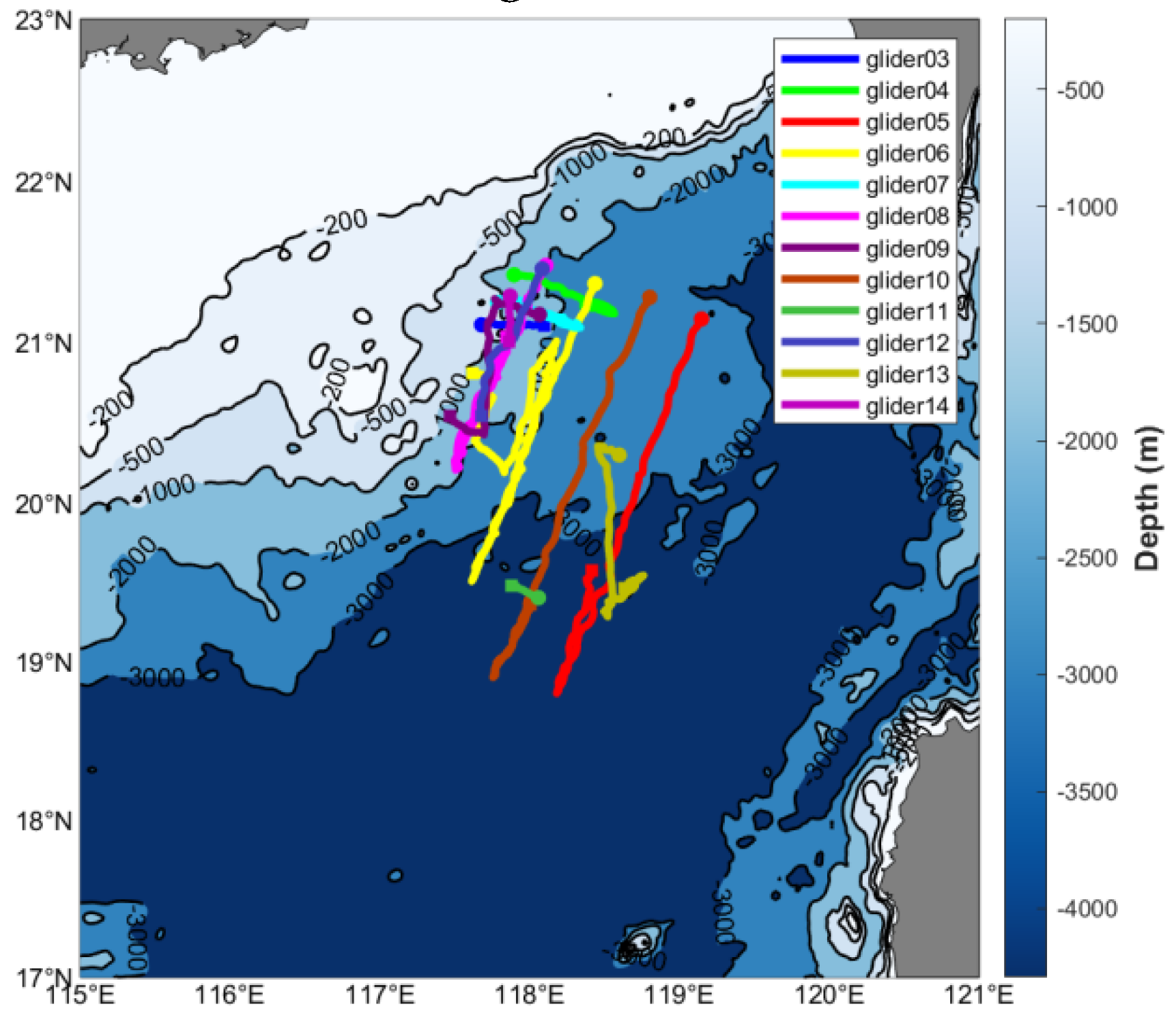
Figure 2.
The movement trajectory of the AE, with black dots representing the daily positions of the eddy center. Critical events including the eddy's generation time, the operational period of underwater gliders, the typhoon passage time, the completion of glider missions, and the eddy's dissipation time are all marked by distinct red dots.
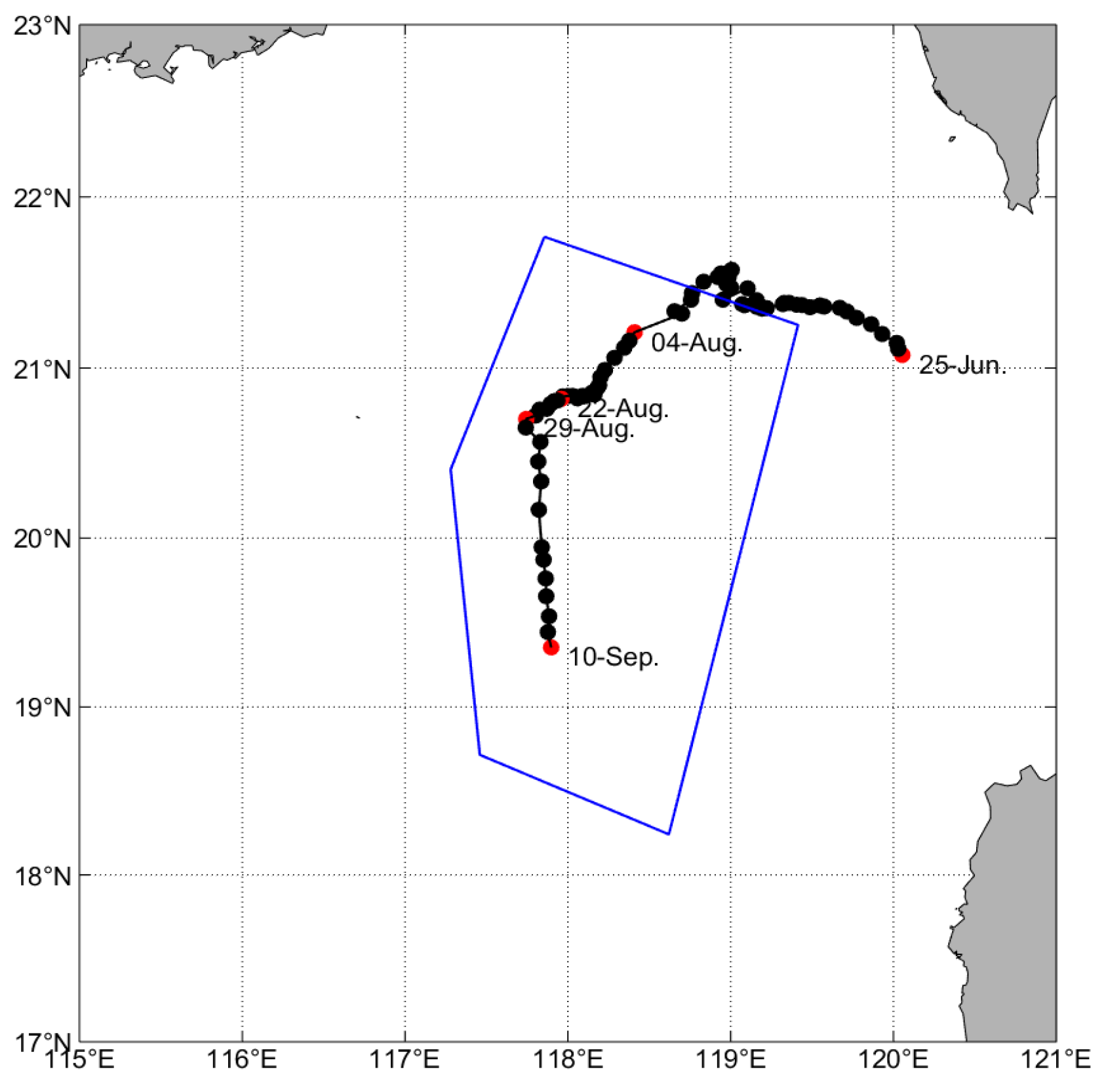
Figure 3.
The development of the AE, with the background representing SSHA and geostrophic current fields derived from satellite altimeter data. The red closed contour indicates the boundary of the AE identified using the WA method.
Figure 3.
The development of the AE, with the background representing SSHA and geostrophic current fields derived from satellite altimeter data. The red closed contour indicates the boundary of the AE identified using the WA method.
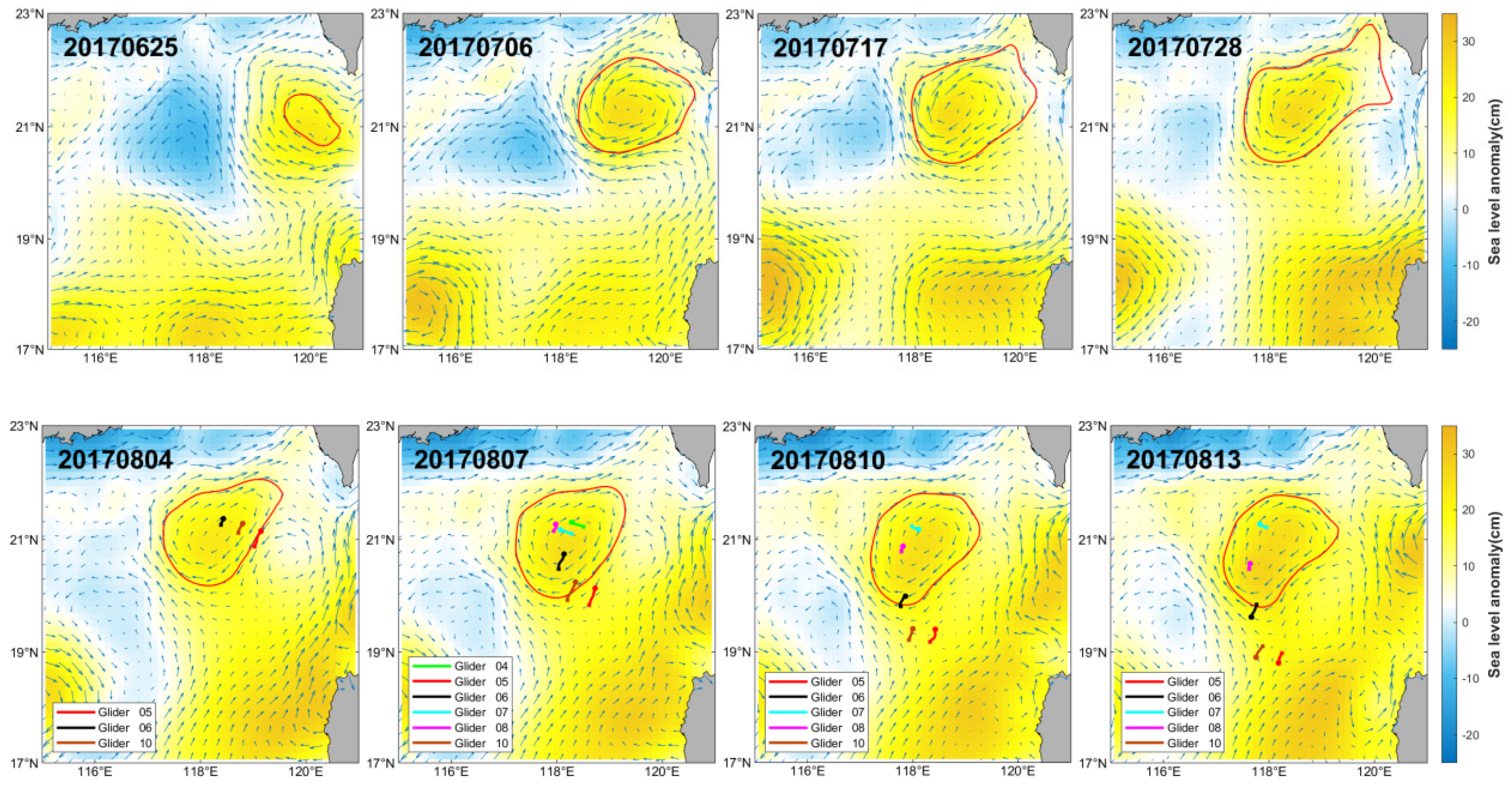
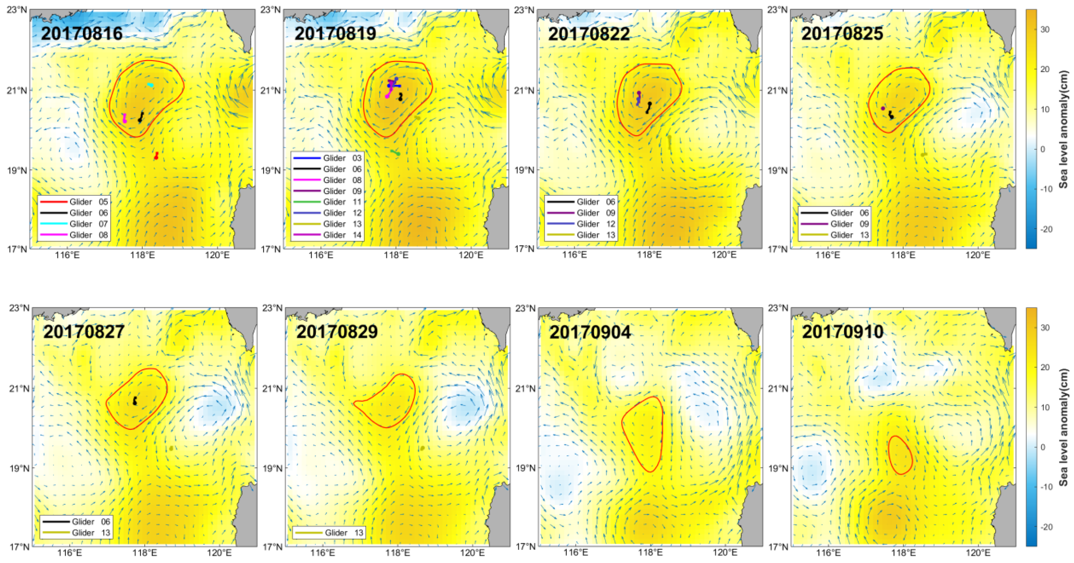
Figure 4.
Temporal evolution of the AE's properties, with vertical line segments indicating the timing of typhoon passages near the eddy: (a) eddy radius; (b) eddy amplitude; (c) eddy kinetic energy.
Figure 4.
Temporal evolution of the AE's properties, with vertical line segments indicating the timing of typhoon passages near the eddy: (a) eddy radius; (b) eddy amplitude; (c) eddy kinetic energy.
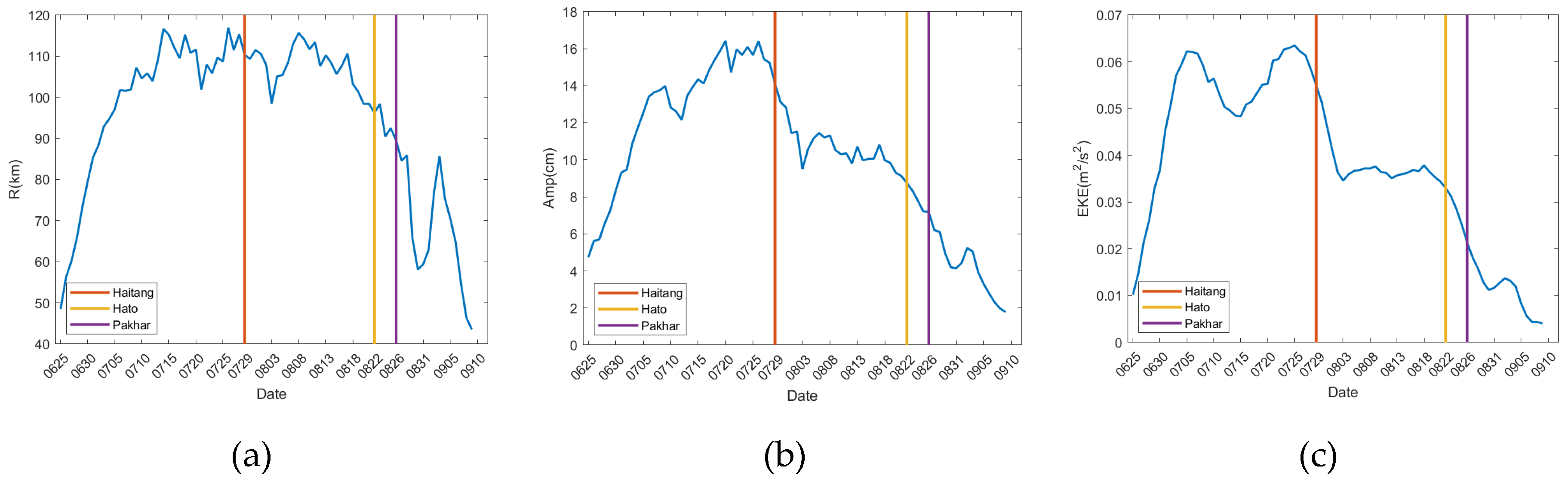
Figure 5.
Horizontal distribution of (a) temperature and (b) salinity across depth layers synthesized from all underwater glider observations.
Figure 5.
Horizontal distribution of (a) temperature and (b) salinity across depth layers synthesized from all underwater glider observations.
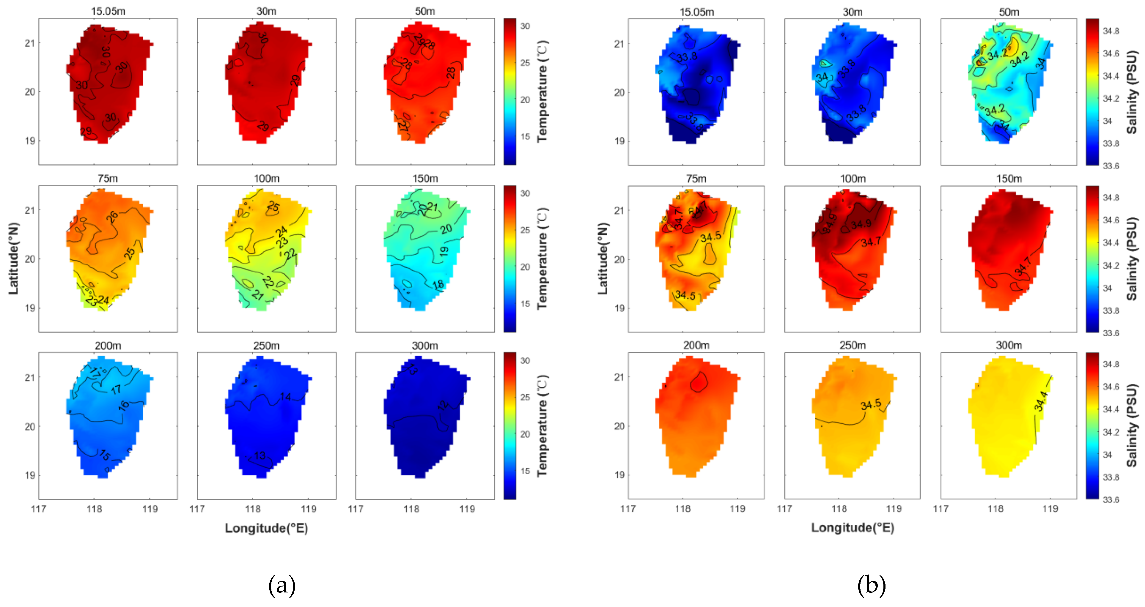
Figure 7.
(a) Temperature and (b) salinity profiles from Gliders 05, 06, and 10. The horizontal axis represents profile sequence numbers along each glider's trajectory, with data collected on August 5 bounded between two black vertical line segments. The red vertical line marks each glider's crossing of the eddy boundary (left: eddy interior; right: exterior).
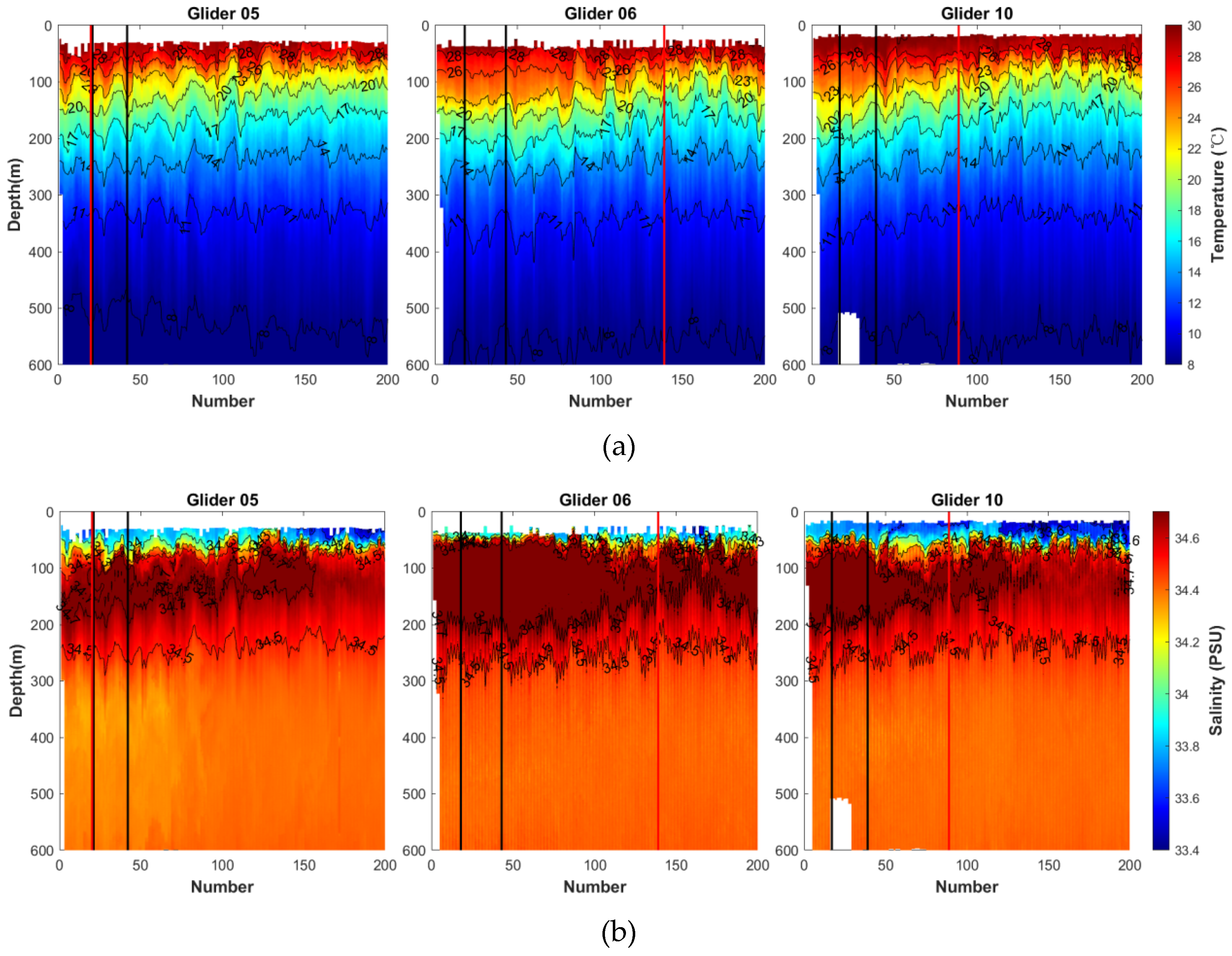
Figure 8.
Comparative analysis of temperature and salinity profiles from Gliders 05, 06, and 10 on August 5: (a) temperature-depth profiles ; (b) temperature differences (ΔT) between Gliders 06, 10 and Glider 05; (c) salinity-depth profiles ; (d) salinity differences (ΔS).
Figure 8.
Comparative analysis of temperature and salinity profiles from Gliders 05, 06, and 10 on August 5: (a) temperature-depth profiles ; (b) temperature differences (ΔT) between Gliders 06, 10 and Glider 05; (c) salinity-depth profiles ; (d) salinity differences (ΔS).
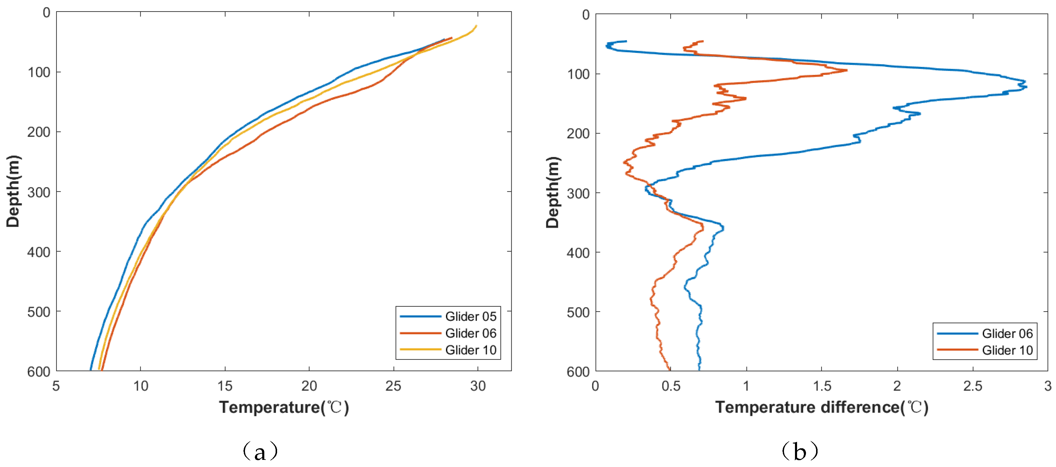

Figure 9.
Trajectory of Typhoon Hato (black curve) with annotated numbers indicating date and hour, superimposed on SSHA (background). The red contour denotes the AE boundary on 22 August. Typhoon intensity classification follows China Meteorological Administration standards, represented by point size and color (see legend). Operational glider numbers are annotated with corresponding typhoon intensity abbreviations during the observation period.
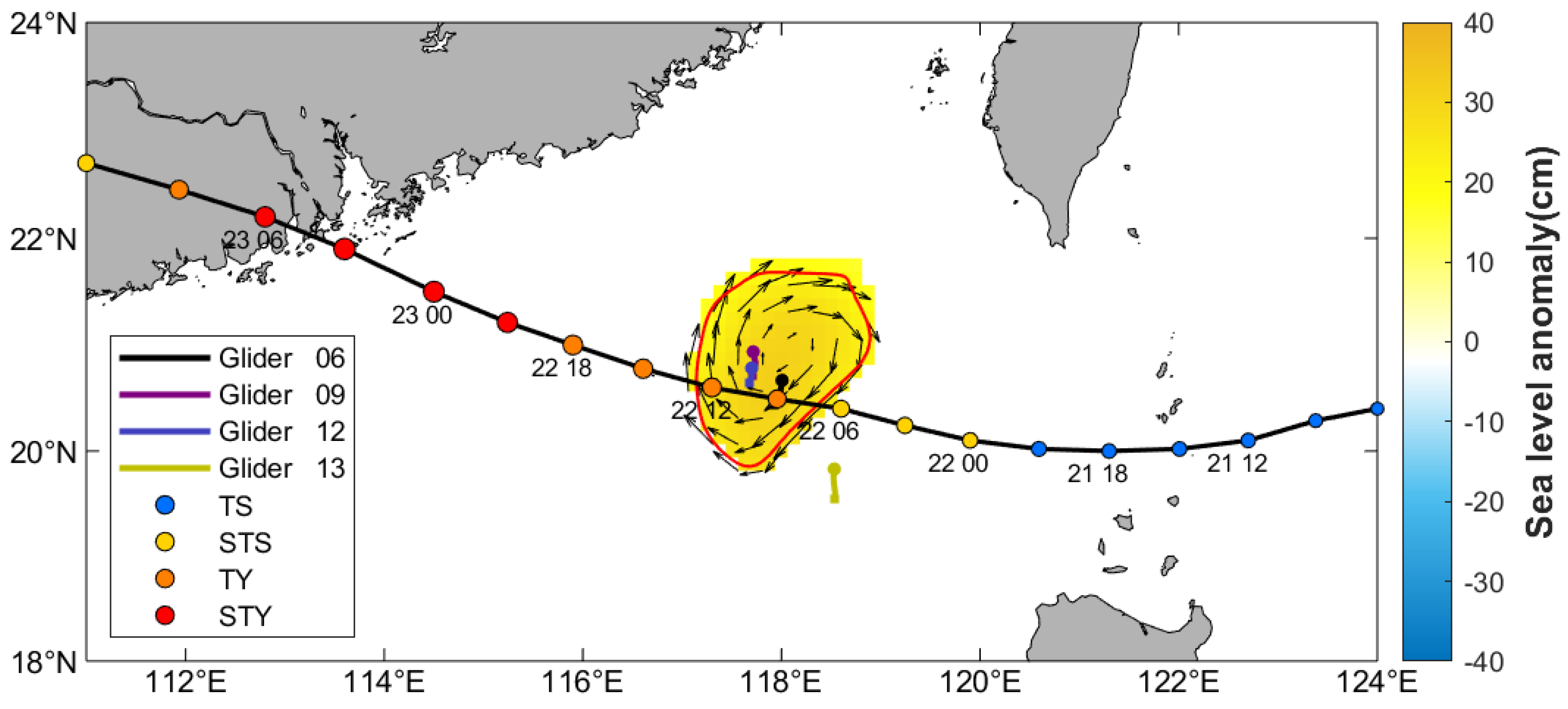
Figure 10.
Thermohaline structure within the AE during typhoon passage, derived from filtered glider profiles to remove high-frequency fluctuations: (a) temperature and (b) salinity distributions from Glider 06 (21-26 August) and Glider 09 (21-25 August).
Figure 10.
Thermohaline structure within the AE during typhoon passage, derived from filtered glider profiles to remove high-frequency fluctuations: (a) temperature and (b) salinity distributions from Glider 06 (21-26 August) and Glider 09 (21-25 August).
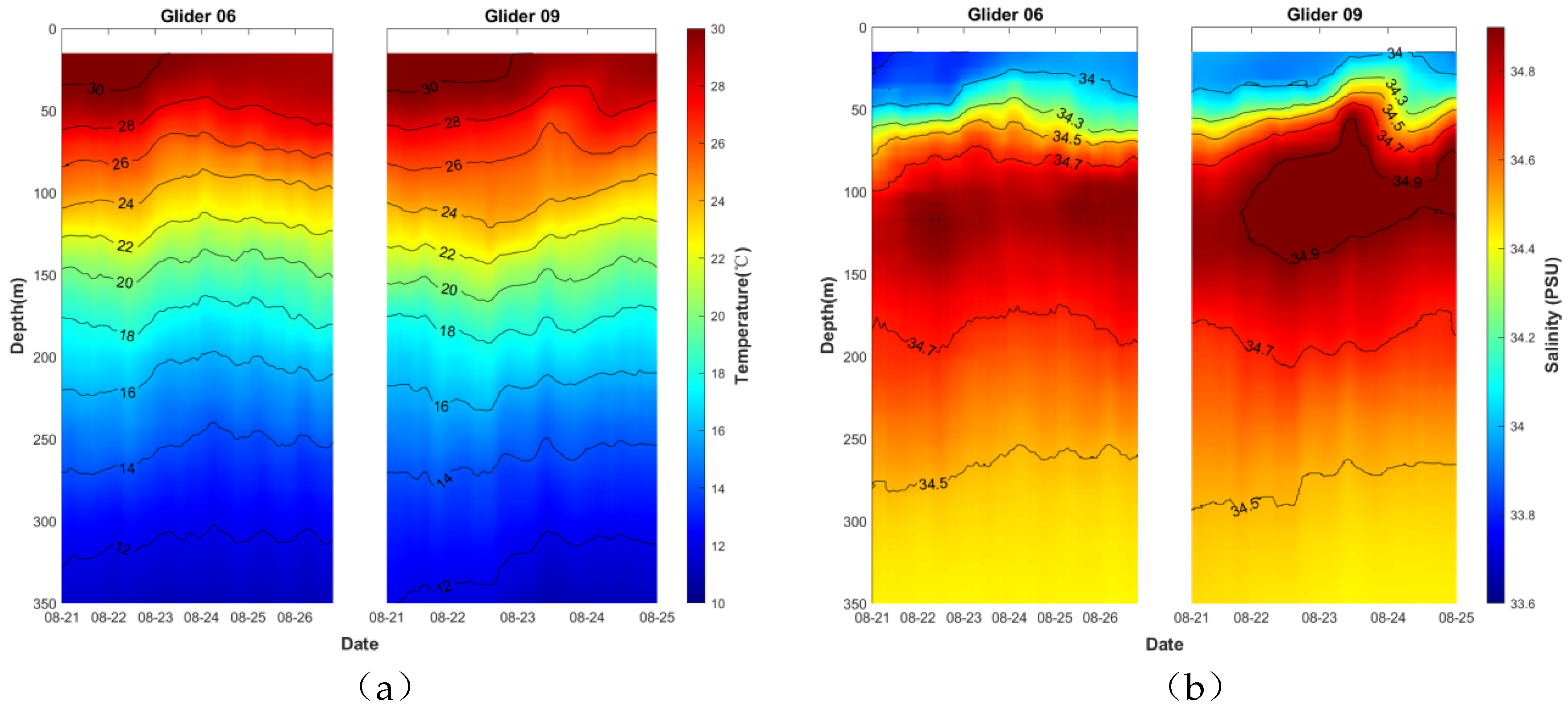
Figure 11.
Eddy-glider spatial relationship analysis: (a) Absolute distances showing temporal variations in eddy radius (blue curve) and Glider 06's distance from eddy center (orange curve) during 15-28 August. (b) Normalized relative distance (glider distance/eddy radius) revealing consistent sampling positions within the eddy's dynamic framework.
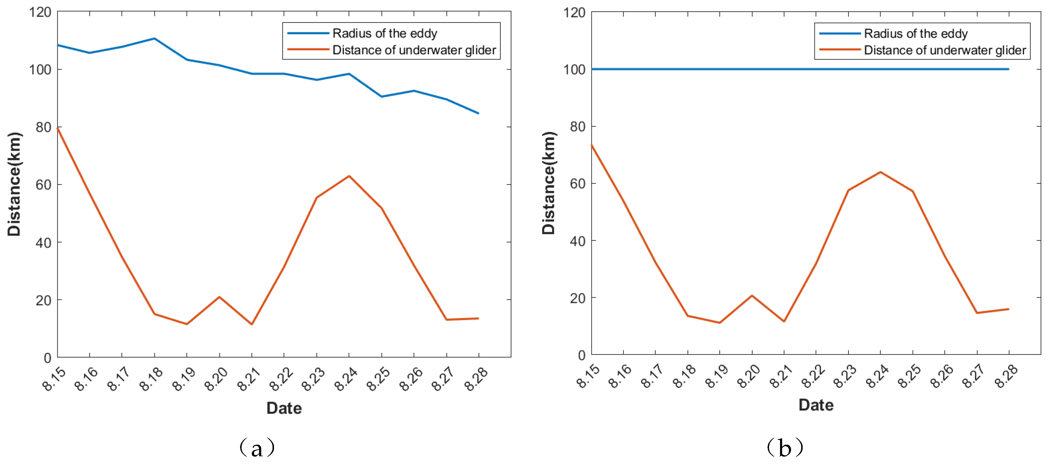
Figure 12.
Thermohaline evolution observed by Glider 06 during Typhoon Hato's passage and recovery phases: (a) Temperature-depth profiles on key dates (22, 23, 25, 27 August); (b) Temperature anomalies relative to position-matched control days (22 vs 17 August, 23/25 vs 16 August, 27 vs 18 August); (c) Salinity-depth profiles; (d) Salinity anomalies.
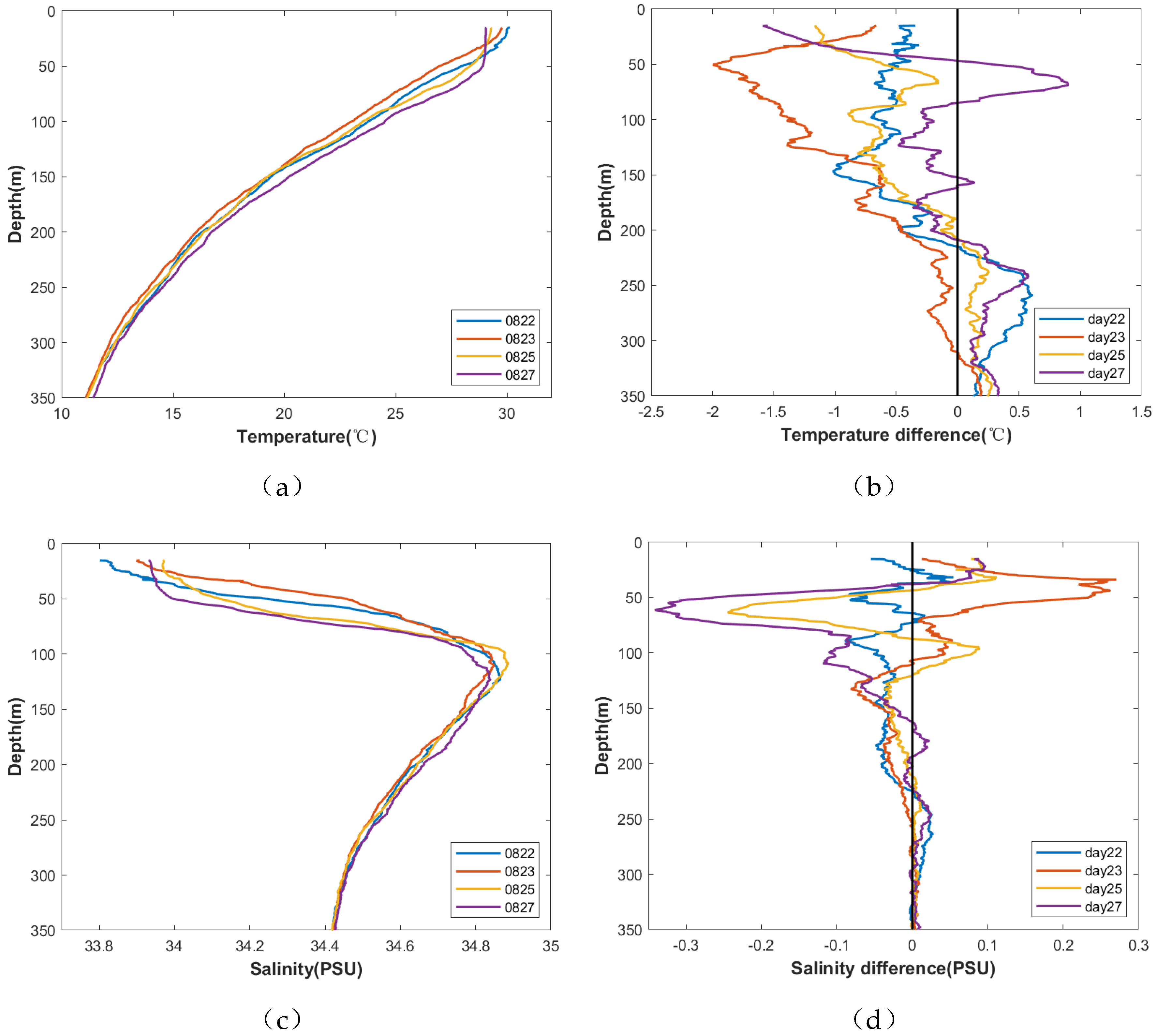
Figure 13.
Comparative wind fields on 22 August from dual numerical experiments: (a) Original ERA5 reanalysis data incorporating Typhoon Hato's complete wind structure; (b) Modified typhoon-free wind field where the typhoon-affected zone was replaced with the average wind in the SCS on that day, while preserving peripheral synoptic patterns.

Figure 15.
Evolution of surface EKE and ζ derived from surface current fields during typhoon passage (21-24 August). (a) EKE distribution; (b) ζ fields documenting the injection of positive vorticity.
Figure 15.
Evolution of surface EKE and ζ derived from surface current fields during typhoon passage (21-24 August). (a) EKE distribution; (b) ζ fields documenting the injection of positive vorticity.
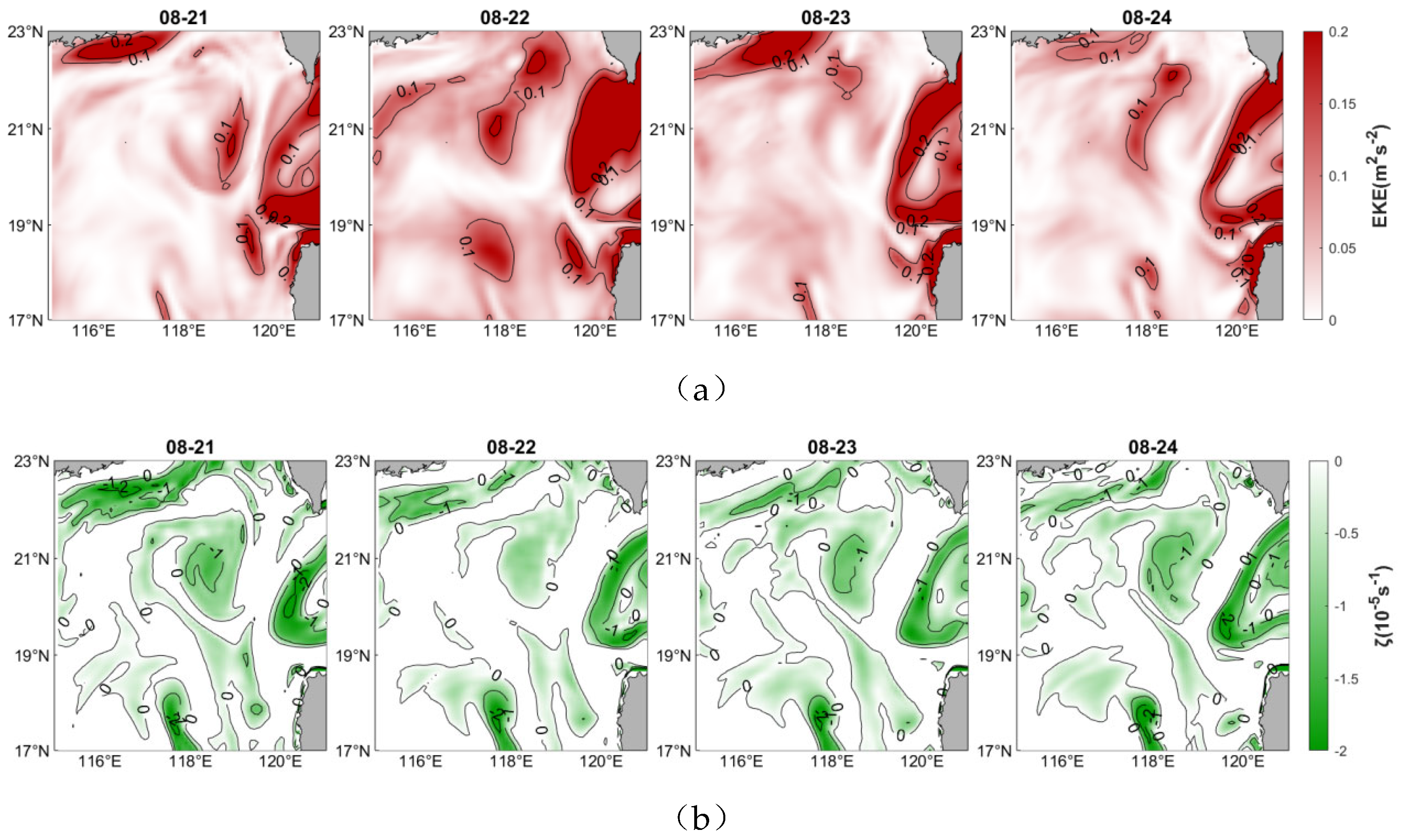
Figure 16.
Surface EKE and distributions under typhoon-free conditions (21-24 August), derived from numerical simulations with climatological wind forcing. (a) EKE distribution; (b) ζ fields documenting the injection of positive vorticity.
Figure 16.
Surface EKE and distributions under typhoon-free conditions (21-24 August), derived from numerical simulations with climatological wind forcing. (a) EKE distribution; (b) ζ fields documenting the injection of positive vorticity.

Figure 17.
Simulated SSHA and AE structure on 20 August (pre-typhoon baseline). The black transect line, aligned latitudinally through the eddy center at (118.5°E, 20.7°N), defines the reference section for analyzing subsequent vertical thermohaline changes.
Figure 17.
Simulated SSHA and AE structure on 20 August (pre-typhoon baseline). The black transect line, aligned latitudinally through the eddy center at (118.5°E, 20.7°N), defines the reference section for analyzing subsequent vertical thermohaline changes.
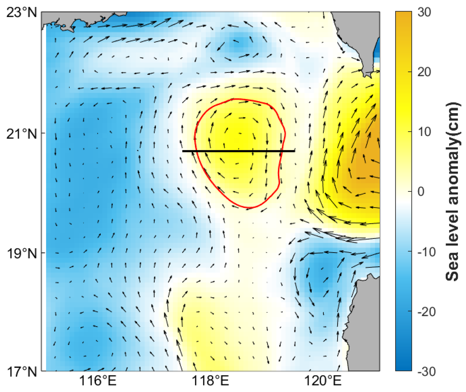
Figure 18.
Simulated vertical velocity cross-sections through the AE center (along 20.7°N), comparing typhoon-forced (a) and background (b) conditions during 21-24 August. Positive values (yellow) indicate upwelling, negative (blue) downwelling.
Figure 18.
Simulated vertical velocity cross-sections through the AE center (along 20.7°N), comparing typhoon-forced (a) and background (b) conditions during 21-24 August. Positive values (yellow) indicate upwelling, negative (blue) downwelling.
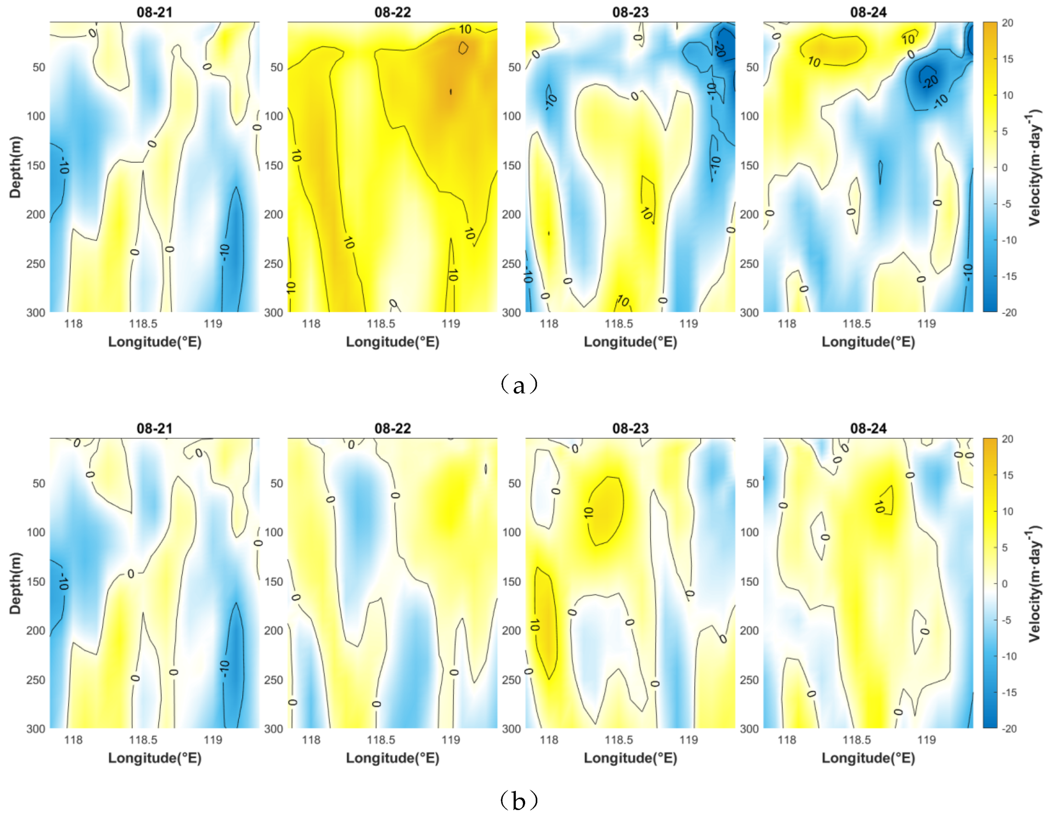
Figure 19.
Simulated temperature evolution in the typhoon experiment along the AE's central transect (aligned with 20 August eddy center position). (a) Temperature profiles from 21-24 August; (b) temperature anomalies relative to 20 August.
Figure 19.
Simulated temperature evolution in the typhoon experiment along the AE's central transect (aligned with 20 August eddy center position). (a) Temperature profiles from 21-24 August; (b) temperature anomalies relative to 20 August.
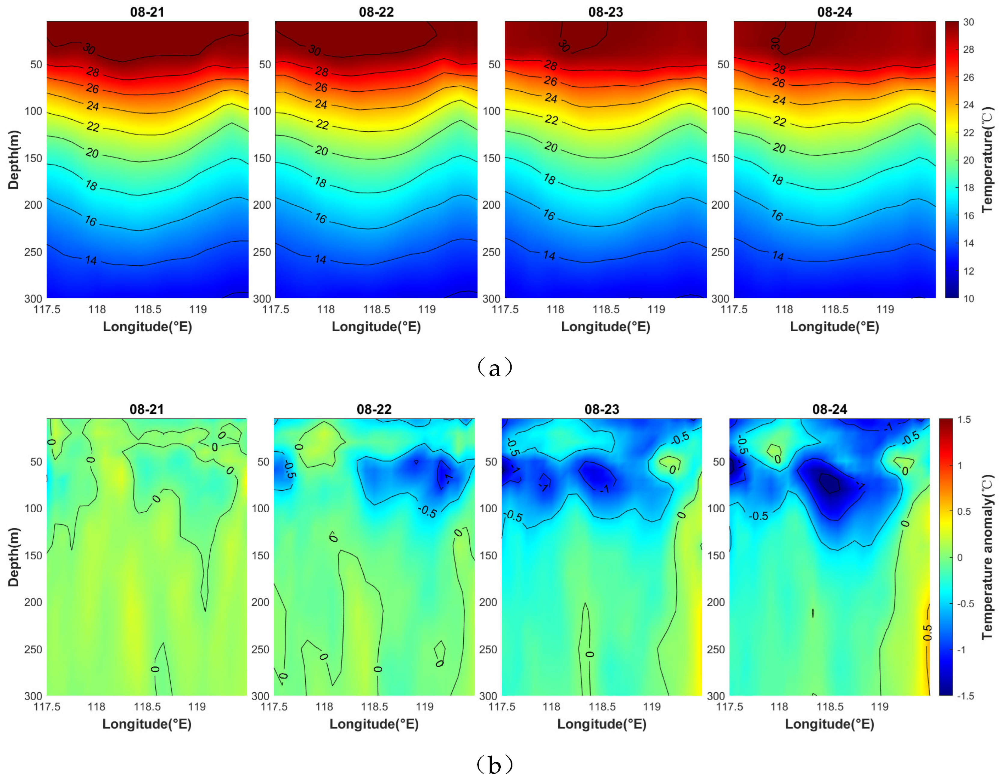
Figure 20.
Simulated temperature evolution in the typhoon-free control experiment along the AE's central transect (identical to Figure 19's spatial coordinates). (a) Temperature profiles from 21-24 August; (b) temperature anomalies relative to 20 August.
Figure 20.
Simulated temperature evolution in the typhoon-free control experiment along the AE's central transect (identical to Figure 19's spatial coordinates). (a) Temperature profiles from 21-24 August; (b) temperature anomalies relative to 20 August.
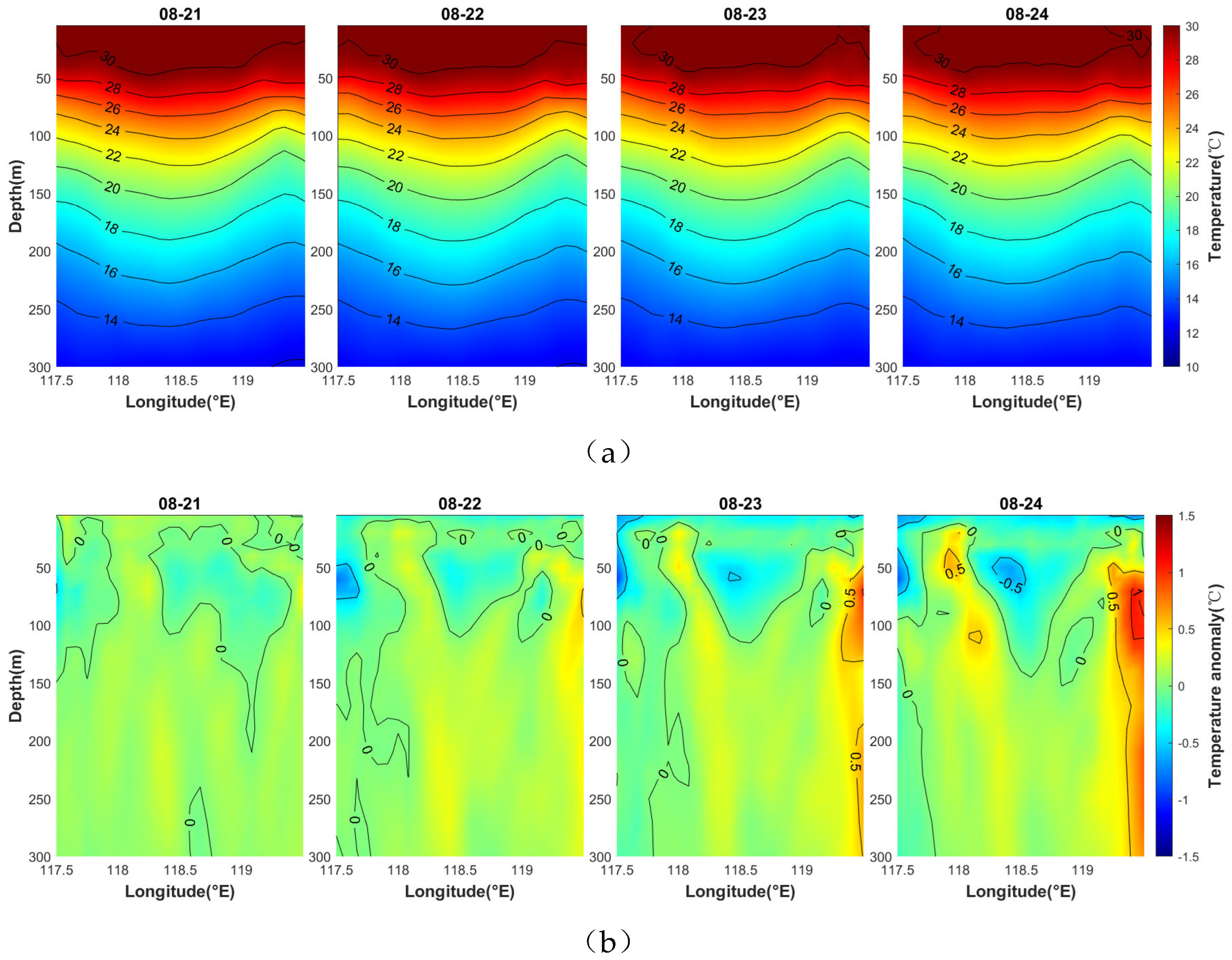
Figure 21.
Simulated salinity evolution in the typhoon experiment along the AE's central transect (aligned with 20 August eddy center position). (a) Salinity profiles from 21-24 August; (b) salinity anomalies relative to 20 August.
Figure 21.
Simulated salinity evolution in the typhoon experiment along the AE's central transect (aligned with 20 August eddy center position). (a) Salinity profiles from 21-24 August; (b) salinity anomalies relative to 20 August.
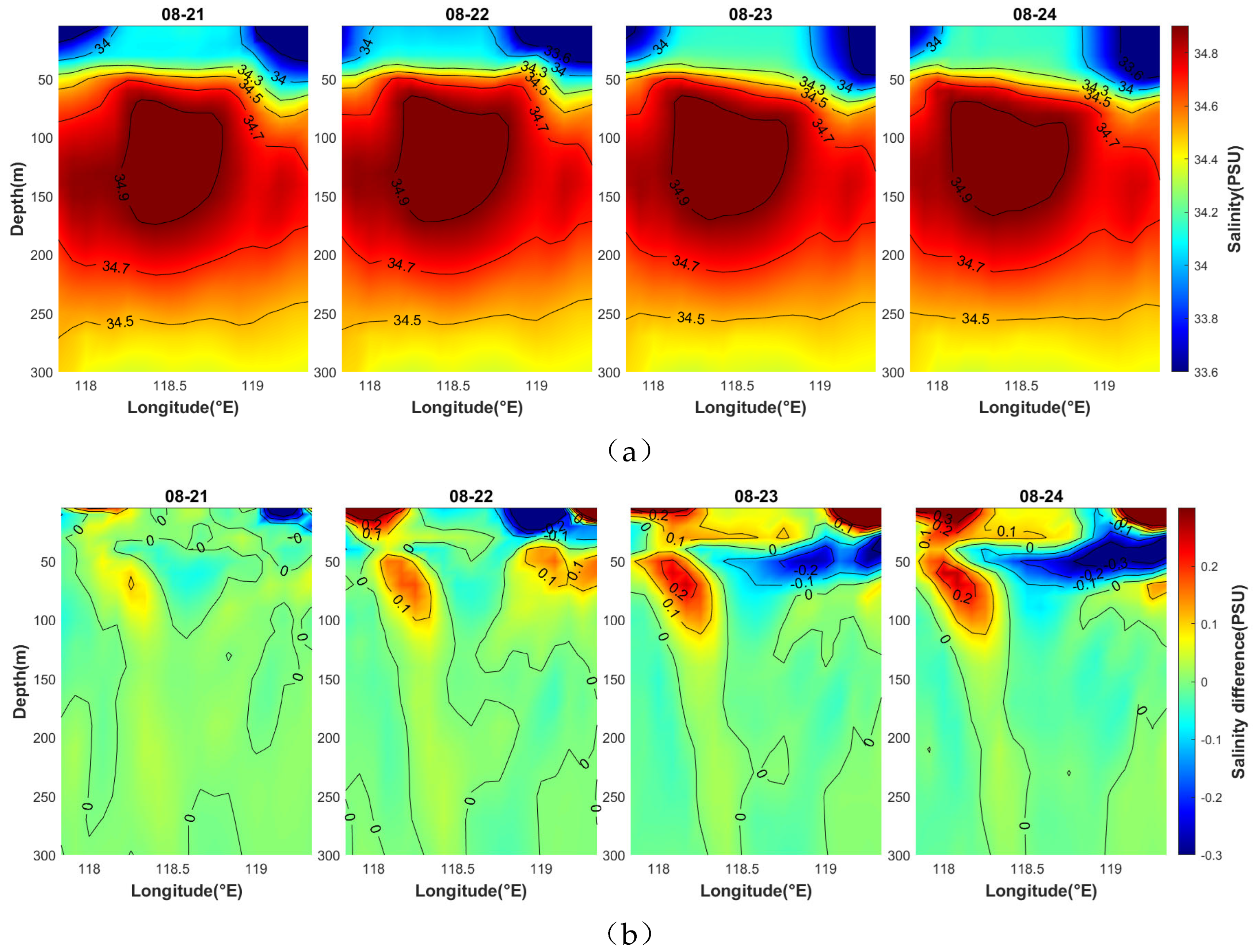
Figure 22.
Simulated salinity evolution in the typhoon-free control experiment along the AE's central transect (identical to Figure 19's spatial coordinates). (a) Salinity profiles from 21-24 August; (b) salinity anomalies relative to 20 August.
Figure 22.
Simulated salinity evolution in the typhoon-free control experiment along the AE's central transect (identical to Figure 19's spatial coordinates). (a) Salinity profiles from 21-24 August; (b) salinity anomalies relative to 20 August.
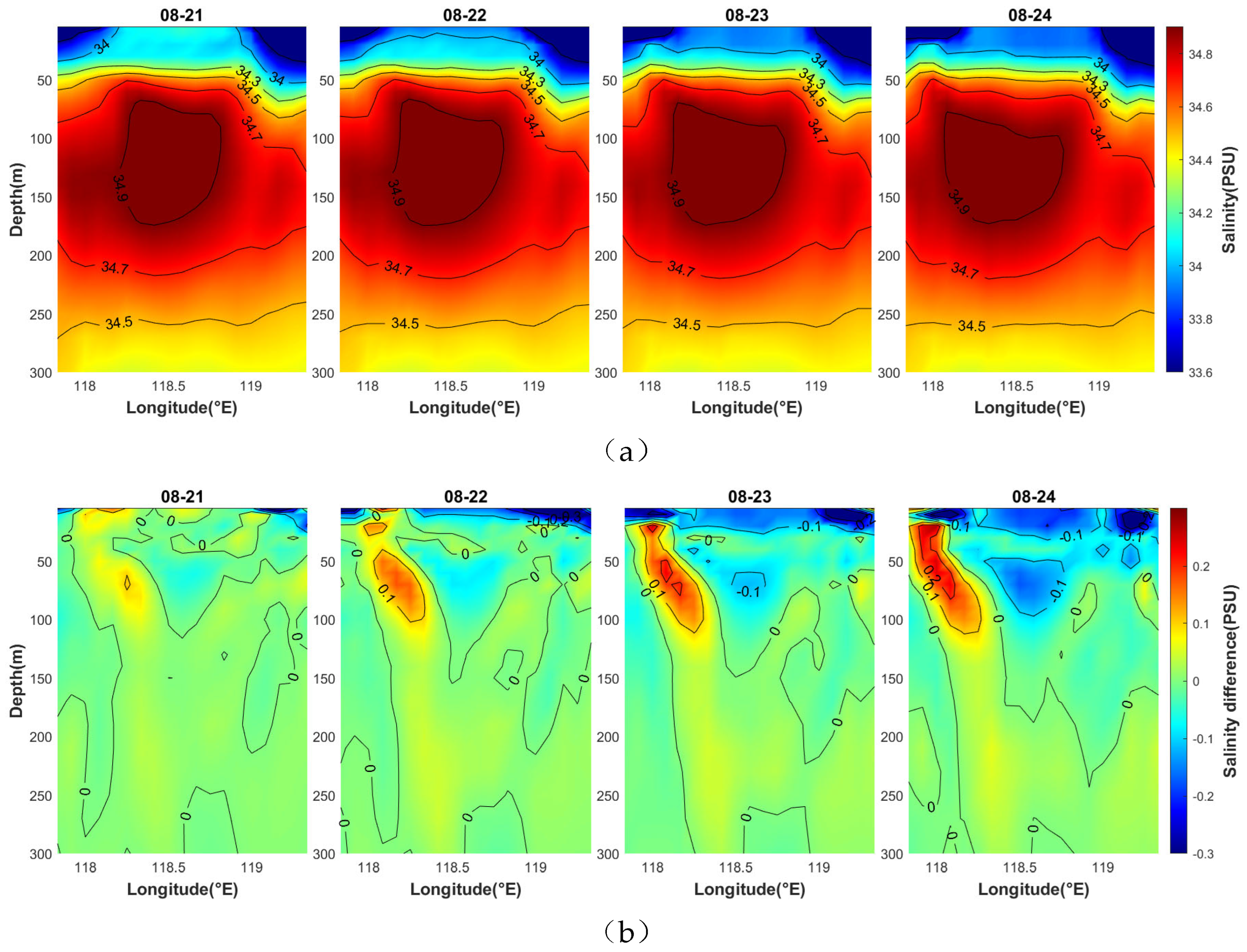
Figure 23.
Vertical structure and current velocity distribution of the AE from 21-24 August, with background colors indicating flow velocity magnitude and eddy identification via the WA method (missing depth layers indicate failed eddy detection). (a) Results from the typhoon-forced simulation; (b) results from the typhoon-free simulation.
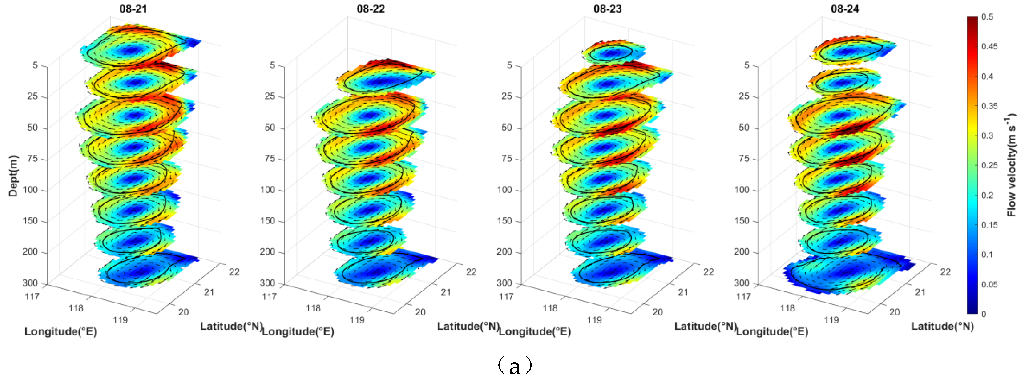
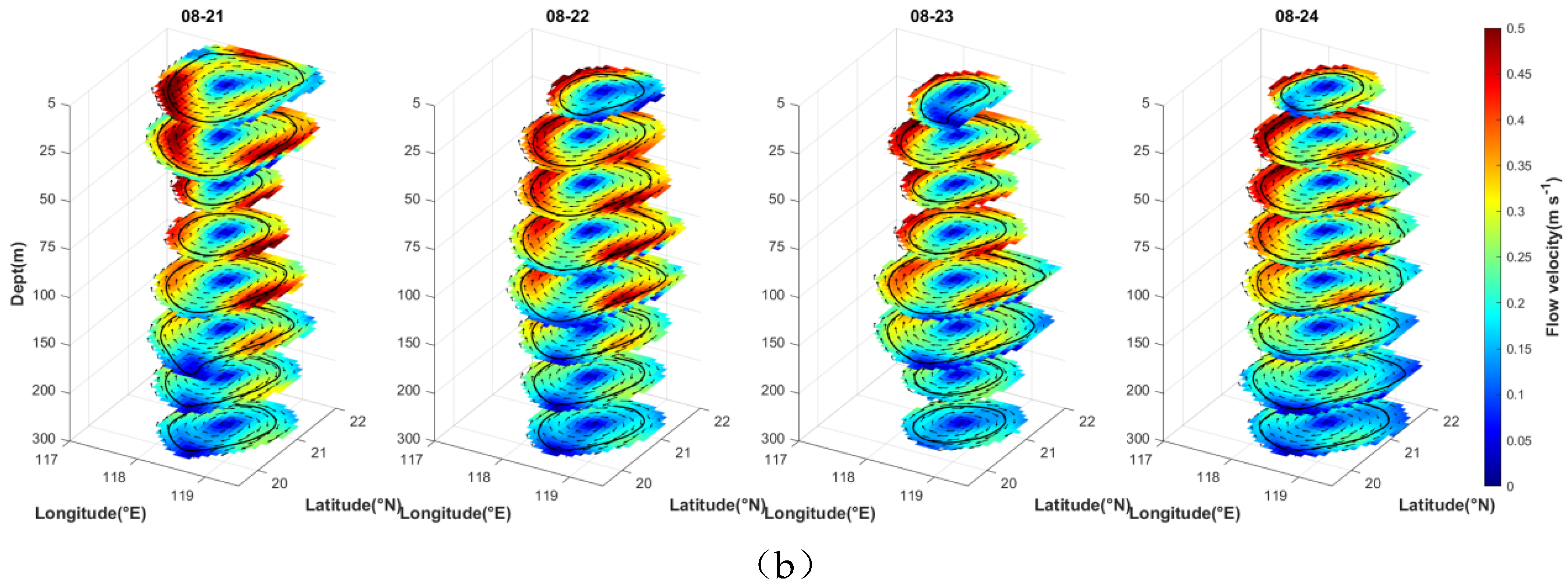

Table 1.
Distance between underwater gliders and the AE center on 5 August 2017.
| Glider ID | Distance from Eddy Center (km) | Relative Position |
| 05 | 78.5 | Eddy boundary |
| 06 | 9.8 | Near eddy core |
| 10 | 46.7 | Intermediate transition zone |
Table 2.
Maximum temperature and salinity differences between Gliders 06, 10 and Glider 05, with corresponding depths.
Table 2.
Maximum temperature and salinity differences between Gliders 06, 10 and Glider 05, with corresponding depths.
| Glider Pair | Max ΔT (°C) | Depth (m) | Max ΔS (PSU) | Depth (m) |
| Glider 06 vs. 05 | 2.86 | 122 | 0.65 | 61 |
| Glider 10 vs. 05 | 1.67 | 94 | 0.14 | 61 |
Table 3.
Maximum temperature and salinity differences below 300 m depth.
| Glider Pair | Max ΔT (°C) | Depth (m) | Max ΔS (PSU) | Depth (m) |
| Glider 06 vs. 05 | 0.85 | 358 | 0.09 | 350 |
| Glider 10 vs. 05 | 0.72 | 361 | 0.07 | 347 |
Table 4.
Comparative analysis of temperature reduction characteristics within the eddy core during the typhoon-affected period for both experimental scenarios.
Table 4.
Comparative analysis of temperature reduction characteristics within the eddy core during the typhoon-affected period for both experimental scenarios.
| Date | 08-21 | 08-22 | 08-23 | 08-24 |
| (TC)Max ΔT (°C) | 0.31 | 1.15 | 1.22 | 1.68 |
| (TC)Depth(m) | 70 | 60 | 60 | 70 |
| (No TC)Max ΔT (°C) | 0.25 | 0.36 | 0.51 | 0.66 |
| (No TC)Depth(m) | 50 | 70 | 60 | 50 |
Disclaimer/Publisher’s Note: The statements, opinions and data contained in all publications are solely those of the individual author(s) and contributor(s) and not of MDPI and/or the editor(s). MDPI and/or the editor(s) disclaim responsibility for any injury to people or property resulting from any ideas, methods, instructions or products referred to in the content. |
© 2025 by the authors. Licensee MDPI, Basel, Switzerland. This article is an open access article distributed under the terms and conditions of the Creative Commons Attribution (CC BY) license (http://creativecommons.org/licenses/by/4.0/).
Copyright: This open access article is published under a Creative Commons CC BY 4.0 license, which permit the free download, distribution, and reuse, provided that the author and preprint are cited in any reuse.


