Submitted:
28 July 2025
Posted:
29 July 2025
You are already at the latest version
Abstract
ANSYS-Fluent was applied to simulate diffusion combustion flame in a two-dimensional (2D) industrial burner to determine the contours of the mass fraction of gas emissions, ve-locity, and combustion temperature. The effects of the boundary conditions, including momentum, thermal, and species (inlet air, inlet fuel, and outlet pressure) on combustion temperature and mass fraction (gas emissions), were analyzed in the designed burner. The present study focused on using and analyzing the volumetric reaction and the turbu-lence-chemistry interaction of the eddy dissipation model for the diffusion flame model of kerosene in the field of combustion. The simulation used the discrete ordinate model and p1 for radiation and the k-e model for turbulence with enhanced wall treatment. Fuel con-sumption reduction was the main positive consequence of using this burner. Based on the results, the magnitude velocities of air and fuel, inlet temperature, and mass fraction of oxygen and inert gas can influence the parameters of flame temperature and gas emissions in the industrial burner. The inlet temperature provided a similar trend for the selected ra-dial positions. Adding the inlet temperature to the combustion chamber can increase flame temperature distributions. By varying the inlet temperature and oxygen mass fraction, the flame configurations on temperature, CO2, and H2O form a symmetry flame. The tempera-ture distribution resulted in the centerline being hotter than other radial positions for all the inlet temperatures. The emissions of CO2 and H2O generally rise with the addition of the oxygen mass fraction.
Keywords:
ANSYS Fluent
; combustion
; flame
; eddy dissipation model
; diffusion flame
1. Introduction
A challenge of combustion is a numerical simulation. Combustion research investigated the gas emissions of NOx and CO using 2D axisymmetric burners for methane-air diffusion flame combustion mode [1] and the numerical analysis of the partially-premixed burner for industrial gas turbine combustion application [2,3]. The research used the Eddy Dissipation Model (EDM), a non-premixed and partially premixed flame model, and the simulation of syngas combustion by a non-premixed flame model coupled with the DO approach that showed better agreement than experimental data [4].
In experimental and numerical investigations on the effect of different air-fuel mixing on the performance of a lean liquid-fueled swirl combustor, the numerical results show different temperatures and species fields predicted for the non-premixed and partially premixed models [5]. A numerical study applied the flamelet progress variable approach on the local flame structure for the partially premixed Dimethyl Ether (DME)/air flame. This study obtained excellent results for the temperature and the species mass fraction [6]. Combustion research [7] conducted a large Eddy simulation (LES) of kerosene spray injection in an aeronautic combustor to assess the capability of an energy deposition model and to reduce the chemical kinetic and global spray injection.
A type of burner, burner moderate and intense low oxygen Dilution (MILD), was tested by the eddy dissipation concept [8], a numerical study in a non-premixed micro combustor with different fuel inlet velocities [9], and direct numerical simulation (DNS) in non-premixed MILD combustion. The research investigated auto-ignition, flame propagation, and aspects of the combustion with a lean mixture. Concepts applied preheating and dilution of the reactant mixture to get a higher temperature than the auto-ignition temperature of the used fuel. It utilizes exhaust gas recirculation (EGR) to improve gas emissions and increase combustion efficiency and stability [10]. However, this method also raised the peak flame temperature and NOx. Inert gases from internal gas recirculation (IGR) have been one strategy to reduce NOx emissions. This method can also minimize oxygen use, known with moderate or intense low oxygen Dilution (MILD) and flameless combustion. Both ways can enhance thermal efficiency and decrease gas emissions [11].
A combustion strategy was applied again, using two spray flames with diameters of 10.5 mm and 25 mm to outline the effect of mixing models. CO2 mass fraction for the three models had similar trends by the result value ranging from 0.01 to 0.125 [12]. The mixing model has determined the flame shape, flow, turbulence, temperature, and species compositions. The predictions of the product H2O by different models were similar to predictions on temperature [13]. The reduction of nozzle diameter is one of the other ways to get an optimum operating condition as carried out by [11] in premixed cyclone combustion experimentally and numerically. The nozzle diameter of 30 mm and the equivalence ratio of 0.89 can yield better gas emissions and flame temperature. The research observed sizes of the fuel orifice, air orifice, combustor diameter, and tailpipe diameter were 1 mm and 2 mm, 5.9 cm, and 2.7 cm, respectively, with pipes of three different lengths, 25.4 cm, 40.7 cm, and 56 cm [14].
Making suitable mixtures between reactant flows and surroundings is a technique widely applied by modifying a nozzle geometry. It determines combustion products. Three nozzle types, namely circular, square, and rectangular, were investigated. From the mean velocity contours, using non-circular nozzles can shorten the potential core length by around 33% compared to the circular nozzle [15]. The rectangular nozzle can produce a centerline velocity decay rate higher than the circular nozzle. However, the slot nozzle produces a centerline velocity decay rate higher than both the rectangular and circular nozzles. The research observed eight different nozzle geometries, such as a round, square, cross, eight-corner start, six-lobe daisy, equilateral triangle, ellipse, and rectangle. The effects of nozzle geometry were significant in mean velocities and turbulent quantities [12] and determined the diameter size of droplets. The operating conditions at the size of around 20 mm for the gas turbine application generally were carried out. The small droplet sizes can evaporate much faster than bigger droplets [16].
The heat transfer process inside the burner was analyzed by coupling spray combustion, forced convection on the wall surface, and conduction in the solid with air heated over the wall. The results were that above and below the cone possessed a different behavior. Above the cone, the temperature gradient stimulated a hot flame so that the temperature of fresh air could elevate. However, below the torch, the negative temperature gradient and stable stratification were achieved [17]. The prediction of wall temperature can use multiphysics simulation with large-eddy simulation (LES), conjugate, and radiative heat transfers. The gas temperatures downstream of the burner chamber were cold. It took place when considering the radiation phenomena, and it were close to the adiabatic temperature when close to the combustion centerline. The maximum temperature remained the same because the sudden temperature increased through the flame front influenced by radiation heat transfer [18].
A comparative study tested non-premixed and partially premixed combustion models in a realistic Tay model combustor to identify temperature and species concentration [19]. To reduce gas emissions, a catalyst can also be used to get complete combustion [20]. The flame stability can be achieved by raising the temperature of reactant species which can also change other combustion characteristics of the flame temperature and the quality of gas emissions. As noted, the smaller geometry size of the combustion chamber can shorten the residence time of the combustion reaction of reactants. For better combustion, the residence time should be longer than the chemical reaction time. The rise of the mixture fraction temperature can shorten the combustion chemical reaction time [21,22]. As conducted by a researcher in [23] applied different chamber geometries to simulate species transport and non-premixed combustion model to determine better chamber design. A combustion technique stabilized the combustion flame using a stoichiometry ratio. The reactant mixtures were acetylene, H2, and air [24]. The other ways accelerated combustion chemistry and reduced CO on flame characteristics and chemical kinetics in a swirl gas turbine combustor using Large Eddy Simulation (LES) [25], used non-premixed combustion model and distributed combustion conditions with the methane as a fuel [26]. A study performed the combustion research of the H2/air mixture with CFD modeling for a 3D and 2D computational domain of micro-cylindrical combustor [27]. That was using the eddy dissipation concept (EDC) and the combustion characteristics of the wall and fluid temperature, hydrogen mass fraction, velocity, and also pressure.
This numerical simulation uses a 2D burner for the diffusion combustion flame. Preheating the mixture fraction of the reactants can widen and change the characteristics of the contours of flame temperature, gas emissions, and flame stability. This work aims to test the combustion performances of the designed geometry burner. Three parameters investigated are fuel and air inlet velocities, inlet temperatures, and oxygen concentrations.
2. Burner and Simulation Setups
The mathematical model has considered several assumptions about the chemical and physical processes to solve and yield results in the combustion study cases. Even though simplifications were performed, perfect setups of mathematical forms have to have similar cases in turbulent flames. The fundamental study of current research is to attend to mathematical tools. This study investigated the turbulence-chemistry interaction of the eddy dissipation model by solving the general transport equations of mass, momentum, energy, and species concentrations.
The combustion chamber for the current work is shown in Figure 1. The sizes of which are 100 cm in length, 50 cm in diameter, 2 cm in fuel injection, and 3 cm in air injection. The computational grid used triangle methods together with three-edge refinement around fuel and air inlets. The max face size, minimum size, and size function are 2 x 10⁻³ m, 1.333 x 10⁻⁴ m, and curvature, respectively, with which obtained the numbers of 146,973 nodes and 291,830 elements. To simulate the governing equations of mass, momentum, energy, and heat transfer for diffusion combustion flame models that are using FLUENT-ANSYS software. The pressure-velocity coupling uses a SIMPLE algorithm with a second-order upwind scheme to discretize the governing equations. The other solver setting with the gradient evaluation used the least-squares cell method. The momentum and energy use second-order upwind. The turbulent kinetic energy and turbulent dissipation rate use first-order upwind. The scale residuals for convergence are 1 x 10⁻⁶ for continuity, energy, and species mass fractions.
The boundary conditions were C12H23 as fuel and air as an oxidizer, consisting of 21% oxygen and 79% nitrogen. The inlet magnitude velocities of the fuel tested were 0.01, 0.03, 0.05, 0.075, 0.1, 0.3, 1, 5, and 10 m/s. The constant of the used air was 0.5 m/s. At the exit combustion chamber, a fixed pressure of 0 Pa was specified, and by choosing stainless steel as the combustion chamber material walls. The boundary conditions of the inlet fuel, inlet air, walls, and pressure in the current study are described in more detail in Table 1. The setup of the simulation is shown in Table 2. The simulation used an Intel (R) Core (TM) i5-7400 CPU @ 3.00 GHz and an installed RAM of 8 GB.
3. Numerical Combustion Model
Most combustors in industrial applications operate using the concepts of spray and reactive flows within the turbulent regime characterized by high Reynolds numbers. The simulation of multi-component fuel spray requires better treatment concepts to yield good turbulence within both the liquid and gaseous phases [28]. The oxy/air-fuel flow in many combustion systems is turbulent. The other types are laminar and transition. The transition flow exists between those two regimes. The turbulent flow is more complex mathematically than both of the flows [29].
3.1. Transport Equation and Chemical Model
The mathematical concept of fluid inside the combustion chamber is described by a set of governing equations (1-4) for mass, momentum, species, and energy in Cartesian coordinates, respectively:
where is the air-fuel mixture density, u is the velocity vector, and T is the mixture temperature. is the mass fraction of species , is the thermal diffusivity, is the specific heat at a constant pressure of species , and is the heat source terms due to chemical reaction. is the correction velocity of species i. The sear stress takes place due to a velocity gradient. The stress tensor equation (5) is
where is the air-fuel dynamic viscosity, is the identity matrix, and is the transpose operation. The Lewis number (Eq. 6), the specific heat at a constant pressure of the air-fuel mixture (Eq. 7), and the correction velocity (Eq. 8), respectively, are calculated with the following equations
where is the local mean molecular weight of the air-fuel mixture, is the mass diffusivity of species . The Schmidt number is the ratio between viscosity and diffusion, . The Prandtl number is the ratio between viscosity and heat transfer, . The Schmidt and Prandtl numbers are due to .
The combustion process in the combustor can influence the flow field through the density parameter. The equation of state for ideal gases expresses the density, . The local heat release rate (Eq. 9) and the relation between the enthalpy and the temperature (Eq. 10) are
The specific enthalpy of species can be expressed as the sum of formation enthalpy at a reference temperature ,
and the heat capacity of the gas mixture for the temperature range between To and the actual value T.
For the Combustion reaction model, the field of chemistry concerning the reaction rate is called chemical kinetics. The chemical reaction rate, , is the decrement change in concentration of the air-fuel reactant () to the gas emissions as combustion products at the time per time ().
For the combustion process the concentration of the fuel and air as the reactants depends on time. That always decreases with it, and the concentration of the combustion products as reaction results always increases with time. With this, the concentration of reactants always has a negative sign. For complete combustion reactions without involving N2 and some inert gaseous, the main chemical reaction (Eq. 14) inside the combustion chamber and the fuel consumption rate (Eqs. 15 and 16) can be determined as
The p and q calculated investigated the depending on the initial consumption rate and initial concentrations of Fuel and oxygen. The sum of n and m is as an overall reaction order. Computing the combustion rate constant (Eq. 14) that can use the following Arrhenius equation (13)
where A, z, p are the frequency factor, the collision frequency, the steric factor (p < 1), respectively, and is the collision fraction at sufficient energy to produce a chemical reaction. Eq. (17) can be rewritten as
Eq. (13) can also be expressed in the logarithmic form (Eq. 15) to find each of the variables
Which is identically a linear equation, Where slope and intercept.
Assuming the chemical equilibrium of gaseous emissions with a complete combustion reaction is occurring without involving N2 and some inert gases, the equilibrium constant inside the combustion chamber (Eq. 16) is
For the complete reversible reaction, the equilibrium rate constant at the left side, as described in equation (17), is
From the ideal gas, , the relation between pressure and concentration is
The equilibrium constant equations (19-20) are
where and are equilibrium constants in terms of concentrations and partial pressures, respectively. is the sum of the gas emission coefficients, and is the sum of the reactant coefficients.
To describe species equations in the governing equations, which can use either mole fraction (X or mass fraction (Y).
From the gas ideal as described in Equations (21-22), the equation becomes
The combustion reactants can also use the mass fraction (Y) (Eqs. 23-24) to symbolize the concentration of species
3.2. Radiation Model
ANSYS Fluent offers five radiation models: the discrete transfer radiation model (DTRM), the P1-radiation model, the Rosseland model, the surface-to-surface (S2S), and the discrete ordinate model (DOM). It allows for including radiation with or without a participating medium in heat transfer simulations. Heating or cooling the surfaces due to radiation or heat sources within the fluid phase is included in one of the above models. Considering the P-1 radiation model, the simplest problem of the more general P-N model, the influence of geometry configuration on the radiative heat transfer, is used as a numerical model in the current study.
Radiative heat transfer should be included in a numerical simulation when the radiant heat flux is large compared to the heat transfer rate due to convection or conduction [30]. Analysis should consider the radiation model if the combustion temperature is more than 2000 K [27]. The volumetric radiative heat transfer involving walls and the fluid medium is more prominent in the combustion chamber, where the gas emissions participate as a medium. Gas emissions can absorb and emit radiation [31]. The radiative transfer equation (25) for an absorbing, emitting, and scattering medium at position in the direction is
where is the scattering direction vector, s is the path length, a is the absorption coefficient. n is the refractive index, is the scattering coefficient, is the Stefan-Boltzmann constant (5.669 x 10⁻⁸ W/m2. K4), I is the radiation intensity, T is the local temperature, is the phase function, and is the solid angle.
3.3. Diffusion Combustion Flame
The combustion research mode consists of diffusion, premixed, and partially premixed flames. The diffusion flame (non-premixed combustion flame) occurs where oxidizer and fuel are not mixed or enter the combustor with distinct streams [32]. Combustion occurs in the mixing layer, which is very small compared to the combustion system, and the mixing step brings reactants into the mixing zone. Controlling combustion and the chemical reaction is very difficult [29]. The time required for turbulent mixing to occur through convection and diffusion processes is significantly larger than that for most of the combustion chemical reactions. The turbulent mixing and chemical reactions are the rate-limiting processes [33].
The combustion process is simplified to a mixing case where transport equations for one or two mixture fractions are solved. In the diffusion model in ANSYS Fluent, the thermochemistry processes of the mixture fraction between fuel and oxidizer are calculated using PDFs [28]. Applying the diffusion combustion model in ANSYS Fluent, which offers the modeling of secondary stream, empirical secondary stream, and empirical fuel stream. When reactant species of fuel and oxidizer mix in the reaction zone, the chemistry can be determined using the other approaches [28].
The mixing of fuel and oxygen, and the chemical reaction occur at the same time. Therefore, it is the rate of mixing that controls the combustion rate. Depending on the state of the fuel, there are gaseous diffusion combustion, and liquid spray combustion. Gaseous diffusion consists of laminar and turbulent combustion. Depending on the flow condition of the fuel gas discharge into the combustion chamber. Since the process occurs inside the flame, it is a complicated case. The simplifications of differential equations for diffusion flames are
- On the flame surface, fuel and air should mix in a proper ratio. Chemical reactions occur only on the flame surface, and they are instantaneous.
- b. The flows of fuel and air are one-dimensional with uniform velocity. The diffusion of the reactants only takes place along the radial directions.
- c. The mole number does not change in the combustion reactions. The pressure is the same throughout the whole process.
- d. The diffusion of fuel and oxygen in inert gases is regarded as the diffusion of two components. Their diffusion coefficients are equal.
The density and diffusion coefficient (D) of mixed gases do not correlate with temperature, so that both of them are constant in the radial direction .
At constant pressure, , the diffusion coefficient of the two components is . Therefore, the effects of temperature on are small. The value of which is approximated as a constant in the radial direction. According to the above assumptions, the mass fraction conservation equation for component k with the chemical reaction is
Each component as follows
By referring to assumption (b), the parameters are and and for a steady-state diffusion combustion process where , So that the eq. (35) becomes
Note that chemical reaction only takes place on the flame surface by referring to assumption (a), but when the process on the flame surface is not considered,, then by using assumption (d), .
The diffusion velocity is described in the following Equation (30)
The second term on the right side of equation (26) can be simplified by referring to the forms of ( and ) and assumption (e)
For the case of an axisymmetric diffusion flame with the cylindrical coordinate system are used
is not related to when it is axisymmetric. By referring to assumption (b) and neglecting the diffusion throughout the z-direction
Eq. (32) becomes
By substituting Eq. (35) into Eq. (32) is found (Eq. 36)
The diffusion flame equation can be simplified by substituting and equation (36) into equation (31), as formed in equation (37)
where is the mass fraction of component , D is the diffusion coefficient of two components, w is the flow rate of gaseous fuel or oxidizer, z is the distance of a certain plane of the flame from the coordinate of the discharge opening. The concentration fields of fuel and oxygen can be determined by the partial differential equation (38), only that the boundary conditions are different (not including the point on the flame surface, because at point . Thus, two differential equations have to be solved for the distribution of and . Adopting the mathematical method by Back and Schumann, a new variable is defined
where is the radius of the flame surface. The fuel-oxygen ratio calculated by Equation (39)
The concentration distribution function of the fuel inside the flame and oxidizer outside the flame (on each plane of the flame) can be correlated by the following boundary conditions, as shown in Equations (40-42), where L is the flame height.
4. Results and Discussion
As explained by previous research in [34], referring to some research conclusions, the spray flame depends on the nozzle, fuel, burner, and operating parameters. The diffusion combustion flame model, coupled with energy, p1 for the radiation model, and k-epsilon for the viscous model, is used to determine the combustion performance of a burner. The contours of the temperature and gas emissions are used as references to evaluate the combustion characteristics of this current work, as performed by previous work in [3]. For the high combustion temperature, gas emissions react with each other to form emission products. Therefore, the parameters under various conditions are an essential parameter to be investigated [3,27,28,31,36]. CO2 indicates complete combustion, whereas HC and CO indicate incomplete combustion [39]. The temperature of a cone is plotted along the axial axis at the radial axis of the centerline. That confirms the symmetry of the simulation result inside the combustion flame [17].
Each fuel has limits to burn (called flammability limits), so that the magnitude of velocities chosen in this work must cover the combustible ranges of the used fuel. The flammability limit of fuels depends on parameters such as temperature, pressure, fuel type, ignition source, and others, but that is not absolute. The lower and upper flammability limits of the kerosene are 0.65 and 1.45, respectively [16].
4.1. Influence of the Velocity Magnitude of Air and Fuel Inlets
Figure 2 presents the contours of temperature with the inlet temperature, and the mass fraction of oxygen in the inlet flow of fuel and air was kept constant at 300 K and 0.21%. As shown by Figure 2, the higher contour temperature for the same conditions is taking place at the magnitude velocity of the inlet fuel of 0.05 m/s in comparison to all of the others. As is expected from this measurement, the temperature along the centerline is low and does not show a constant value. It is also shown that the temperatures at axial distances from 0 cm to 50 cm, on the other hand, are more uniform and higher. This result is a little different from the previous research work in [3], where the temperature along the centerline showed a constant value of 1775 K, indeed at axial distances > 80 mm. The plots of temperature for the reference case in Figure 2 show that the maximum temperature takes place in the flame zone, namely around the centerline of the combustion chamber, as indicated in [40].
The temperature along the axial distances at various radial distances shows a constant value of 1200 for the axial distance >200 mm indeed. The flame shape for all cases is predominantly symmetric about the y=0 mm plane with respect to the centerline of the combustion chamber for all axial distances towards the outlet. The results agree with the experiments in [36,41]. Some research results have obtained an asymmetric flame shape or disagreed with the symmetric flame, as mentioned in [3]. The case of the transition from symmetric to asymmetric flame shape is seen in the present simulation of the NO mass fraction. By increasing fuel velocity, which can enhance the entrainment of flue gas, as well as the high velocity, can lead to a large amount of entrainment of flue gas, which can create a lower O2 concentration [42]. This result is different from the previous research, where the temperature of the centerline in the combustion zone and preheat zone increased slightly by applying a microporous combustor [43].
The H2O contours, as shown in Figure 3, under various air magnitude velocities, with the fuel velocity magnitude kept constant at 0.5 m/s. The inlet temperature was kept constant at 300 K by using the mass fraction of oxygen of 0.21. The maximum mass fraction of H2O takes place almost near the inlet air at all of those magnitudes of velocity. The complete combustion requires enough oxygen, which is provided near the air inlet. The location close to the air inlet is in good agreement with the other mass fraction results. A more visible discrepancy is noticed at the far-field location, as explained by the higher predicted temperature. The characteristics of the H2O flame contour are different at each of the various magnitude velocities and are very lovely at 0.0005 m/s.
The temperature contours inside the combustion chamber are not uniform, so the evaluation of temperature contour uniformity is usually needed by determining the pattern factor (PF). The parameter, which is defined by Eq. (52), is determined by measuring the homogeneity of the combustion chamber temperature and the maximum temperature contour. The value of PF is closer to 1, which indicates that the outlet temperature contour distribution of the combustion chamber is more uniform [40].
where Tin is the average inlet temperature of both air and fuel, is the maximum temperature at the combustor outlet, and is the average temperature contour at the outlet combustion chamber of the burner.
The flame contour area of radial velocity, as displayed in Figure 4 at a magnitude velocity of 0.1 m/s (inlet temperature =300oC), is better than the other contour. For the boundary condition at the inlet fuel of 0.01 m/s and temperature of 700 K, the radial velocity of 0.25-0.75 m/s dominates the flame contour with an area of more than 47%, and the maximum radial velocity is 1.93 m/s with the flame contour area of around 2.5%. For the boundary condition at the inlet fuel of 0.1 m/s and temperature of 300 K, the velocity of 0.5-1.4 m/s dominates the contour, with the area about 45% and the radial velocities of 3-4 m/s are about 5% of the flame contour area. The velocity of 0 m/s to 1 m/s dominates the flame contour with an area of more than 70% of the boundary condition at the inlet fuel of 0.1 m/s and temperature of 300 K. The radial velocities of 4 m/s to 5 m/s are around less than 5% of the flame contour area for this condition.
Figure 5(a-5d) are displaying the mass fraction of CO. An asymmetric curve for all the fuel inlets and four axial distances is almost formed. The lowest CO is obtained at the fuel inlet of 1.5 m/s. The concentration of CO is lower than that of the other cases of fuel inlets. At the centerline of radial position, CO gets a significant decrease for all the cases except for the case of B. The lower CO indicates a better combustion process for the operating condition, and it is expected to take place to achieve a higher temperature. CO is an intermediate product of gas emission formed and further oxidized into CO2. A chemical combustion reaction between air and fuel results in the following products: and . CO can be detected in flue gases. It is due to the following reasons, such as not enough residence time for both the air and fuel to react and burn in a combustor. The burner chamber is too cold. The air-fuel ratio is out of stoichiometry (the ideal mixing ratio). The fuel and air in a burner chamber are insufficiently mixed [34,35].
Figures (5e-5h) are the CO2 mass fraction versus radial and axial distances for various boundary conditions of fuel inlet at a constant air inlet of 0.5 m/s. Both the temperature fuel and temperature air inlets are kept at 300 K. The curves for all the fuel inlets and four axial distances form a symmetric curve with a similar trend when the radial distance of 0 m is used as a centerline. The curves obtained almost resemble the CO mass fraction. The highest CO2 mass fraction is obtained at the fuel inlet of 0.05 m/s by the highest concentration of around 0.52%. With the centerline of radial position, CO2 shows a significant decrease in all the cases. The higher CO2 indicates a complete combustion process for the operating condition. The characteristic of the CO2 contour is close to all of those. CO2 forms near the oxygen inlet because at this place, where the oxygen provided is more than at the wall and the center of the combustion chamber. This current research agreed with previous work in [46].
4.2. Influence of Inlet Temperature
In this section, the volume fraction of oxygen is kept constant at 0.21% with an air velocity of 0.5 m/s. The mass fraction and magnitude velocity of kerosene kept constant are 1% and 0.01 m/s, respectively. The effects of the inlet temperature of fuel and air on temperature distribution inside the combustion chamber at 500 K, 700 K, 900 K, and 1500 K are as shown in Figure 6. The increase of which can raise the combustion chamber temperature to all the selected radial positions. The maximum temperature occurs at the inlet temperature of 1500 K, followed by 900 K, 700 K, and 500 K. The chemical reaction occurs rapidly at a higher temperature, and the mixing of fuel and oxygen is faster [32]. The increment of the maximum temperature from 500 K to 900 K is 280 K, from 1573 K to 1853 K. However, it is 170 K from 1853 K to 2023 (lower at 700 K to 900 K). Furthermore, from 900 K to 1500 K, the increment is higher, 375 K from 2023 K to 2398 K. This is due to the higher inlet temperature, which results in more uniform temperature distribution. A similar result is shown in reference [42]. The configuration of flame forms a symmetry flame, which occurs at the radial positions of 0.1 m and -0.1 m for the temperature inlet. The temperature distributions at the centerline and close to the combustor centerline are hotter for all the inlet temperatures than at other radial positions. However, that is colder when far from the centerline. This yield differs from the research in [18].
The inlet temperature addition of 500 K to 1500 K can raise the CO mass fraction, as shown in Figure 7. The trend of the CO curve is very smooth, like taking place on temperature profiles in Figure 6. CO at the radial position of 0 m is prominent and significantly decreases up to 0.2 m axial distance. However, at the other radial positions, the values increase significantly, occurring for all the inlet temperatures. The levels of CO emission are almost constant at the axial distances > 0.4 m. The temperature range from 300 K to 1800 K corresponded to the prediction of CO, whereas the oxidation of CO dominated at temperatures above 1800 K [47].
Figure 8 displays CO2 mass fraction curves versus the axial direction at varying inlet temperatures from 500 K to 1500 K. Increasing inlet temperature can decrease the CO2 mass fraction for all radial positions. This result differs from the research in [34,37]. The trend of the CO2 curve is almost similar to that of H2O. The CO2 decreases in all the radial directions except at d=0 m. The emission of CO2 is more significant than CO because the concentration of oxygen is more dominant in forming CO2 than other emissions. The level of CO2 can change significantly up to the axial distances of 0.2-0.4 m because the oxygen is still more available around the positions. CO2 is almost constant at the axial distances > 0.4 m for all the cases. The curves of CO2 for all inlet temperatures under the radial positions of 0.1 m and -0.1 m show slight differences and form a symmetrical flame. Figure 9 shows the H2O mass fraction by blowing up air and fuel contours. The H2O mass fraction almost forms a symmetry flame configuration. The higher H2O concentration is obtained at the air inlet because forming this gas emission requires enough oxygen. The rise in inlet temperature can increase the CO2 level, but it is not significant.
4.3. Influence of Oxygen Mass Fraction
The current analysis compares previous research and simulation results. Results display different study fields of various oxygen mass fractions. The velocity magnitude and inlet temperature of air kept constant are 0.5 m/s and 300 K, respectively. For the fuel inlet, the values provided are kept at 0.01 m/s and 300 K, respectively. Figure 10 shows the effect of oxygen on temperature distribution inside the combustion chamber under various boundary conditions of the oxygen from 0.21% to 0.8 %. Know that increasing the oxygen concentration can raise contour temperatures. The higher oxygen concentration can result in a more uniform temperature distribution by yielding perfect combustion. The simulation results are similar to reference [42]. Said that the oxygen reduction can affect the field of temperature as a research in [26] by applying various oxygen concentrations of 21%, 18%, and 15%. The results agree with a reference [47] for the temperature contour, with the radial position of 0.2 m closer to the wall temperature.
This simulation not only provides the flame temperature distribution contours as a result of the combustion process, but also provides the gas emissions, as presented in Figure 10 and Figure 11. The effects of oxygen are that the emissions of H2O and CO2 increase, while the emissions of CO and NO decrease. The predicted gas emission results agree well with theory. The addition of oxygen level forms CO decreases, and CO2 increases because the perfect combustion takes place with enough oxygen [44,48]. The rise of temperature and oxygen for a stoichiometric burning can increase the amount of CO2 [39]. The results of NOx and CO decreased up to nearly zero, but CO2 increased slightly under the oxygen concentrations of 18% and 15% by volume [26]. The formation of NOx depends upon reaction duration, inlet temperature, and oxygen availability in the combustor [49]. NOx is reduced by dual-stage low premixed (DLF) flame technology because DLF controls combustion temperature by limiting the use of the equivalence ratio of premixed gas [50]. The level of NOx is dependent on the oxygen concentrations, and the CO emission is dependent on the air-fuel ratio [51].
Carbon monoxide (CO) is available in combustion gas as a result of the partial oxidation of carbon content in fuel. The presence of which in gas emission is an indication of low combustion efficiency because it is not completely oxidized to CO2. The form of which can reduce the thermal combustion efficiency, of course, which can increase fuel consumption. CO is present more when the combustion process is carried out with too little air than required stoichiometry, and therefore, the oxygen is insufficient for completing carbon oxidation reactions. The combustion process occurs with excess air/oxygen higher than the stoichiometric requirement [52].
The geometric size of the combustion chamber influences gas emissions. The emission of CO is higher for a small combustion chamber than for a large combustion chamber [48]. The higher temperature of the flame, which appears in forming H2O and CO2, is more dominant because the synthesis of the emissions yields an enthalpy of the combustion reaction higher than that of CO. Oxygen provided must be more than required to increase fuel conversion efficiency to gas emissions. The emissions of CO2 and H2O, as shown in Figures 11 (a-d), generally increase with the addition of the oxygen mass fraction at all the selected lines, except in the case of Figure 11d. The highest CO2 and H2O emissions take place for the cases of Figures 11C and 11L, respectively. Those cases describe the complete combustion for these operating conditions and can be used in the real application, as proved by the flame temperature in Figure 10. The flame configuration of CO2 and H2O almost forms a symmetrical shape, especially when the axial position is less than 0.25 m. The values of CO2 range from more than 0 to 0.6, which are more similar to the results in [12].
For an excellent understanding, Figure 12 displays the flame temperature contours at various oxygen mass fractions. The addition of oxygen mass fraction can increase the flame temperature in the combustion chemical reaction. That can change contour form, contour area, and flame stability of temperature. For the same oxygen concentration, as shown in Figure 12 (a-b), it is obvious that both have sharp differences. Saying the temperature contour in Figure 12b gives better results with the area of 2061 to 2400oC, which is wider than those of Figure 12a. The condition, as shown in Figure 12b, involves an inert gas of CO that can react with enough oxygen to form CO2. Another reason for this case is to predict the effect of the transport direction of O2 species on the near fuel distribution by an Injector.
The perfect combustion is more serious, taking place near the fuel injector area. The explanations proved, as shown in Figure 12c, are forming a sharp difference when the presence of CO is neglected in the case of Figure 12d. The condition in the case of Figure 12d just only involves CO2 and H2O, so that the temperature contour shows enough difference compared with the cases of Figure 12 (b-c). Displaying also that temperatures near the fuel inlet are more significant than the air inlet. The temperatures near the nozzle are generally higher for both axial and radial temperature profiles; those results agree well with previous research in [3].
5. Conclusions
The simulation results of operating conditions of various inlet temperatures, magnitude of velocity, and the mass fraction of oxygen are compared with the prior research results. The given tests to the combustion chamber using kerosene fuel have resulted in better performance when applying inlet velocity magnitudes for fuel=0.01 m/s and air=0.5 m/s. The flame shape for all the cases of inlet velocity is predominantly symmetric about the y=0 mm for all the axial distances towards the outlet. The maximum mass fraction of H2O takes place almost near the inlet air at all of those magnitudes of velocity. The characteristics of the H2O flame contour are different at each of the various magnitude velocities and very lovely at 0.0005 m/s. An asymmetric curve for all the fuel inlets and four axial distances forms on the mass fraction of CO, with the lowest CO mass fraction obtained at the fuel inlet of 1.5 m/s. The curves obtained are almost similar to the CO mass fraction. The highest CO2 mass fraction is obtained at the fuel inlet of 0.05 m/s by the highest concentration of around 0.52%. The curves for all the fuel inlets and four axial distances form a symmetric curve with a similar trend when the radial distance of 0 m is the centerline.
The increase of inlet temperature can raise the combustion chamber temperature to all the selected radial positions, and the maximum temperature takes place at the inlet temperature of 1500 K, followed by 900 K, 700 K, and 500 K, respectively. The CO2 curve trend is almost similar to H2O. The increase in the inlet temperature of air and fuel can raise the CO mass fraction, but can decrease CO2. Higher oxygen levels leading to a higher peak temperature in the flame, which can reduce fuel consumption. The inert gas, CO, can widen peak temperature areas. Adding the mass fraction of oxygen can raise the combustion flame temperature and can change the contour form, contour area, and flame stability with temperature. The inert gaseous concentrations can influence gas temperatures and the emissions of CO2, CO, and H2O in the combustion chemical reaction. Adding oxygen, the emissions of H2O and CO2 increase, while the emission of CO decreases. The predicted gas emission results agree well with theory. The highest CO2 and H2O emissions occurs for the cases of C and L, respectively. Those cases can be selected in real applications, as proved by the flame temperature. The emissions of CO2 and H2O form a symmetry flame when the axial position is less than 0.25 m.
Author Contributions
Conceptualization, M and W.C.C.; methodology, M.; software, W.C.C.; validation, W.C.C.; formal analysis, M.; investigation, M.; resources, M.; data curation, M.; writing—original draft preparation, M.; writing—review and editing, W.C.C.; visualization, W.C.C.; supervision, W.C.C.; project administration, W.C.C.; funding acquisition, M and W.C.C. All authors have read and agreed to the published version of the manuscript.
Funding
The authors working on this project have not accepted financial support.
Data Availability Statement
All data needed to support the findings of this research are included within the article.
Conflicts of Interest
The authors declare that they have no conflict of interest.
References
- Saini, R.; Prakash, S.; De, A.; Yadav, R. Investigation of NOx in piloted stabilized methane-air diffusion flames using finite-rate and infinitely-fast chemistry based combustion models. Therm. Sci. Eng. Prog. 2018, 5, 144–157. [Google Scholar] [CrossRef]
- Andreini, A.; Facchini, B.; Innocenti, A.; Cerutti, M. Numerical Analysis of a Low NOx Partially Premixed Burner for Industrial Gas Turbine Applications. Energy Procedia 2014, 45, 1382–1391. [Google Scholar] [CrossRef]
- Greifenstein, J.H.M. , Dreizler, B.B.A.: Experimental Investigation of Global Combustion Characteristics in an Effusion Cooled Single Sector Model Gas Turbine Combustor. Flow Turbul. Combust. 1025. [Google Scholar]
- Law, W.P.; Gimbun, J. Scale-adaptive simulation on the reactive turbulent flow in a partial combustion lance: Assessment of thermal insulators. Appl. Therm. Eng. 2016, 105, 887–893. [Google Scholar] [CrossRef]
- De Giorgi, M.G.; Sciolti, A.; Capilongo, S.; Ficarella, A. Experimental and Numerical Investigations on the Effect of Different Air-Fuel Mixing Strategies on the Performance of a Lean Liquid Fueled Swirled Combustor. Energy Procedia 2016, 101, 925–932. [Google Scholar] [CrossRef]
- Hartl, S.; Messig, D.; Fuest, F.; Hasse, C. Flame Structure Analysis and Flamelet/Progress Variable Modelling of DME/Air Flames with Different Degrees of Premixing. Flow, Turbul. Combust. 2018, 102, 757–773. [Google Scholar] [CrossRef]
- Senoner, L.H.J.M. , Cuenot, A.B.B.: Large-Eddy Simulation of Kerosene Spray Ignition in a Simplified Aeronautic Combustor. Flow Turbul. Combust. 2018. [Google Scholar]
- Lewandowski, M.T.; Ertesvåg, I.S. Analysis of the Eddy Dissipation Concept formulation for MILD combustion modelling. Fuel 2018, 224, 687–700. [Google Scholar] [CrossRef]
- Sarath, C.; Sreejith, M.; Reji, R. Flow Field Predictions of Bluff Body Introduced Micro Combustor. Procedia Technol. 2016, 24, 420–427. [Google Scholar] [CrossRef]
- Anh, N. , Doan, K., Swaminathan, N.: Autoignition and flame propagation in non-premixed MILD combustion. Combust. 2019. [Google Scholar]
- Chanphavong, L.; Al-Attab, K.; Zainal, Z.A. Flameless Combustion Characteristics of Producer Gas Premixed Charge in a Cyclone Combustor. Flow, Turbul. Combust. 2019, 103, 731–750. [Google Scholar] [CrossRef]
- Honhar, P.; Hu, Y.; Gutheil, E. Analysis of Mixing Models for use in Simulations of Turbulent Spray Combustion. Flow, Turbul. Combust. 2017, 99, 511–530. [Google Scholar] [CrossRef]
- Wang, H. , Pant, T., Zhang, P.: LES / PDF Modeling of Turbulent Premixed Flames with Locally Enhanced Mixing by Reaction. Flow Turbul. Combust. 2018. [Google Scholar]
- Anand, V.; Jodele, J.; Knight, E.; Prisell, E.; Lyrsell, O.; Gutmark, E. Dependence of Pressure, Combustion and Frequency Characteristics on Valved Pulsejet Combustor Geometries. Flow, Turbul. Combust. 2017, 100, 829–848. [Google Scholar] [CrossRef]
- Fabiola, G. , Tay, K., Tachie, M.F.: Effects of Nozzle Geometry on Turbulent Characteristics and Structure of Surface Attaching Jets. Flow Turbul. Combust. 2019. [Google Scholar]
- Chrigui, M.; Moesl, K.; Ahmadi, W.; Sadiki, A.; Janicka, J. Partially premixed prevalorized kerosene spray combustion in turbulent flow. Exp. Therm. Fluid Sci. 2009, 34, 308–315. [Google Scholar] [CrossRef]
- Moureau, G.L.V. , Chauvet, S.D.N.: Modeling of Conjugate Heat Transfer in a Kerosene/Air Spray. Flow Turbul. Combust. 2018. [Google Scholar]
- Koren, C.; Vicquelin, R.; Gicquel, O. Multiphysics Simulation Combining Large-Eddy Simulation, Wall Heat Conduction and Radiative Energy Transfer to Predict Wall Temperature Induced by a Confined Premixed Swirling Flame. Flow, Turbul. Combust. 2018, 101, 77–102. [Google Scholar] [CrossRef]
- Zhang, K.; Ghobadian, A.; Nouri, J. Comparative study of non-premixed and partially-premixed combustion simulations in a realistic Tay model combustor. Appl. Therm. Eng. 2017, 110, 910–920. [Google Scholar] [CrossRef]
- Chen, J.; Liu, B.; Yan, L.; Xu, D. Computational fluid dynamics modeling of the combustion and emissions characteristics in high-temperature catalytic micro-combustors. Appl. Therm. Eng. 2018, 141, 711–723. [Google Scholar] [CrossRef]
- Turkeli-Ramadan, Z.; Sharma, R.N.; Raine, R.R. Two-dimensional simulation of premixed laminar flame at microscale. Chem. Eng. Sci. 2015, 138, 414–431. [Google Scholar] [CrossRef]
- Sadiki, A.; Agrebi, S.; Chrigui, M.; Doost, A.; Knappstein, R.; Di Mare, F.; Janicka, J.; Massmeyer, A.; Zabrodiec, D.; Hees, J.; et al. Analyzing the effects of turbulence and multiphase treatments on oxy-coal combustion process predictions using LES and RANS. Chem. Eng. Sci. 2017, 166, 283–302. [Google Scholar] [CrossRef]
- Enagi, I.I.; Al-Attab, K.; Zainal, Z. Combustion chamber design and performance for micro gas turbine application. Fuel Process. Technol. 2017, 166, 258–268. [Google Scholar] [CrossRef]
- Andreini, A.; Bertini, D.; Facchini, B.; Puggelli, S. Large-Eddy Simulation of a Turbulent Spray Flame Using the Flamelet Generated Manifold Approach. Energy Procedia 2015, 82, 395–401. [Google Scholar] [CrossRef]
- Rajpara, P.; Shah, R.; Banerjee, J. Effect of hydrogen addition on combustion and emission characteristics of methane fuelled upward swirl can combustor. Int. J. Hydrogen Energy 2018, 43, 17505–17519. [Google Scholar] [CrossRef]
- Karyeyen, S. Combustion characteristics of a non-premixed methane flame in a generated burner under distributed combustion conditions: A numerical study. Fuel 2018, 230, 163–171. [Google Scholar] [CrossRef]
- Pashchenko, D. Comparative analysis of hydrogen/air combustion CFD-modeling for 3D and 2D computational domain of micro-cylindrical combustor. Int. J. Hydrogen Energy 2017, 42, 29545–29556. [Google Scholar] [CrossRef]
- Afshar, A. : Evaluation of liquid fuel spray models for hybrid RANS/LES and DLES prediction of turbulent reactive flows. 2014. [Google Scholar]
- Fachbereich Maschinenbau, V. , Kumar Goud Pantangi aus Nalgonda, P., Berichterstatter, I., Amsini Sadiki Mitberichterstatter, H., Dinkelacker Mitberichterstatter, F., Johannes Janicka, D.I.: Large Eddy Simulation of Mixing and Combustion in Combustion Systems under Non-adiabatic Conditions. Ph. 2015. [Google Scholar]
- ANSYS Fluent Tutorial Guide, www.ansys.
- Abubakar, Z.; Shakeel, M.R.; Mokheimer, E.M. Experimental and numerical analysis of non-premixed oxy-combustion of hydrogen-enriched propane in a swirl stabilized combustor. Energy 2018, 165, 1401–1414. [Google Scholar] [CrossRef]
- Gao, Y. , Chow, W.K.: A Brief Review on Combustion Modeling. Int. Journ. Architectural Sci. 2005; 6. [Google Scholar]
- Zimmermann, I. : Modeling and Numerical Simulation of Partially Premixed Flames. Ph. 2009. [Google Scholar]
- Guo, F.; Wang, C.; Zhang, A.; Li, M. Study on kerosene spray combustion and self-extinguishing behaviors under limited ventilation. Fuel 2019, 255. [Google Scholar] [CrossRef]
- Örs, I.; Sarıkoç, S.; Atabani, A.; Ünalan, S.; Akansu, S. The effects on performance, combustion and emission characteristics of DICI engine fuelled with TiO2 nanoparticles addition in diesel/biodiesel/n-butanol blends. Fuel 2018, 234, 177–188. [Google Scholar] [CrossRef]
- Arshad, S. , Adhiraj, E.G., Suresh, D., Oevermann, M.: Subgrid Reaction-Diffusion Closure for Large Eddy Simulations Using the Linear-Eddy Model. Flow Turbul. Combust. 2019. [Google Scholar]
- Masjudin; Chang, W. -C. Combustion performance of the premixed and diffusion burners with used lubricating oil and used cooking oil as fuel. Mod. Phys. Lett. B 2019, 33. [Google Scholar] [CrossRef]
- Michel, O.C.J. : A Two-Dimensional Tabulated Flamelet Combustion Model for Furnace Applications. Flow Turbul. Combust. 2016; 97. [Google Scholar]
- Bayındır, H. , Is, M.Z.: Evaluation of combustion, performance and emission indicators of canola oil-kerosene blends in a power generator diesel engine. Appl. Therm. Eng. 2017. [Google Scholar]
- Krieger, G.; Campos, A.; Takehara, M.; da Cunha, F.A.; Veras, C.G. Numerical simulation of oxy-fuel combustion for gas turbine applications. Appl. Therm. Eng. 2015, 78, 471–481. [Google Scholar] [CrossRef]
- Ma, L. , Xu, H., Wang, X., Fang, Q., Zhang, C., Chen, G.: A novel flame-anchorage micro-combustor : Effects of flame holder shape and height on premixed CH4/air flame blow-off limit. Appl. Therm. Eng. 1138. [Google Scholar]
- Zhu, S.; Pozarlik, A.; Roekaerts, D.; Rodrigues, H.C.; van der Meer, T. Numerical investigation towards HiTAC conditions in laboratory-scale ethanol spray combustion. Fuel 2018, 211, 375–389. [Google Scholar] [CrossRef]
- Wang, W.; Zuo, Z.; Liu, J. Numerical study of the premixed propane/air flame characteristics in a partially filled micro porous combustor. Energy 2019, 167, 902–911. [Google Scholar] [CrossRef]
- Baukal Jr, C.E. : Industrial Combustion Pollution and Control. Marcel Dekker Ink., New York U.S. 2004. [Google Scholar]
- Way, T.W. : Industrial Gas Burner. ( 2017.
- Bagheri, G.; Hosseini, S.E.; Wahid, M.A. Effects of bluff body shape on the flame stability in premixed micro-combustion of hydrogen–air mixture. Appl. Therm. Eng. 2014, 67, 266–272. [Google Scholar] [CrossRef]
- Heinrich, A.; Ganter, S.; Kuenne, G.; Jainski, C.; Dreizler, A.; Janicka, J. 3D Numerical Simulation of a Laminar Experimental SWQ Burner with Tabulated Chemistry. Flow, Turbul. Combust. 2017, 100, 535–559. [Google Scholar] [CrossRef]
- Flagan, R.C. , Seinfeld, J.H.: Fundamentals of Air Pollution Engineering. 1988. [Google Scholar]
- Choudhary, K.D. , Nayyar, A., Dasgupta, M.S.: Effect of compression ratio on combustion and emission characteristics of C.I. The engine operated with acetylene in conjunction with diesel fuel. 2018. [Google Scholar]
- Zhao, W.; Qiu, P.; Liu, L.; Shen, W.; Lyu, Y. Combustion and NOx emission characteristics of dual-stage lean premixed flame. Appl. Therm. Eng. 2019, 160. [Google Scholar] [CrossRef]
- Noel, D. , Kushnoore, S., Kamitkar, N., Satishkumar, M.: Experimental Studies of Compression Ignition Diesel Engine Using CNG and Pongamia Biodiesel in a Dual Fuel Mode. Americ. Journ. Mech. Indutr. Eng. 2016; 1. [Google Scholar]
- F. Draught: Buner Handbook. 2001.
Figure 1.
Diffusion burner.

Figure 2.
Radial temperature profile at the axial positions of 0.2, 0.4, 0.65, and 0.9 m with the velocity magnitude of the air inlet of 0.5 m/s and various fuel inlets of: (a) 0.05 m/s; (b) 0.1 m/s; (c) 0.3 m/s; and (d) 1.5 m/s.
Figure 2.
Radial temperature profile at the axial positions of 0.2, 0.4, 0.65, and 0.9 m with the velocity magnitude of the air inlet of 0.5 m/s and various fuel inlets of: (a) 0.05 m/s; (b) 0.1 m/s; (c) 0.3 m/s; and (d) 1.5 m/s.
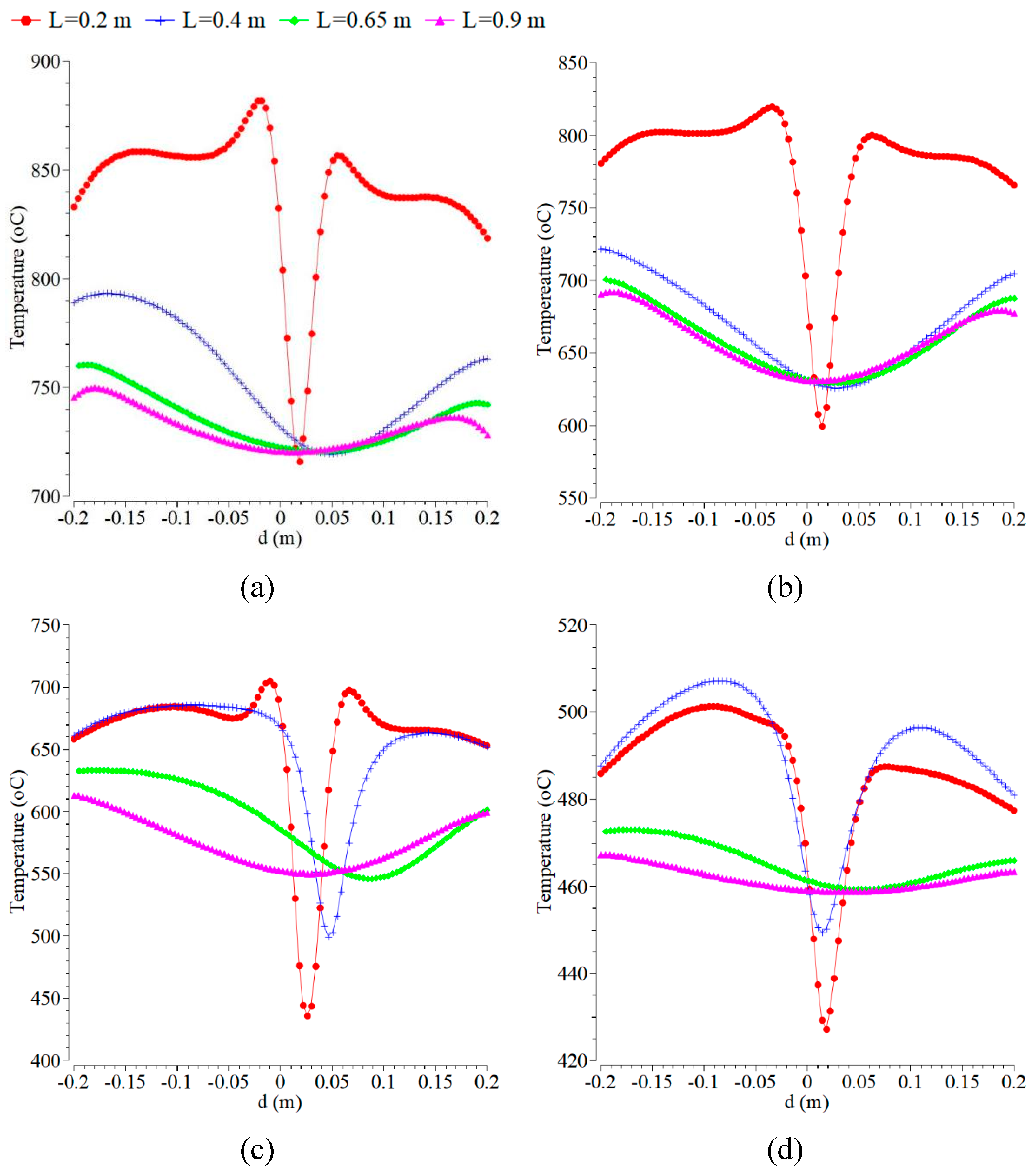
Figure 3.
Comparison of the contour of mass fraction of H2O at the axial positions of 0.2, 0.4, 0.65, and 0.9 m with the velocity magnitude of the air inlet of 0.5 m/s and various fuel inlets: (a) 0.0005 m/s; (b) 0.1 m/s; (c) 0.3 m/s; and (d) 1.5 m/s.
Figure 3.
Comparison of the contour of mass fraction of H2O at the axial positions of 0.2, 0.4, 0.65, and 0.9 m with the velocity magnitude of the air inlet of 0.5 m/s and various fuel inlets: (a) 0.0005 m/s; (b) 0.1 m/s; (c) 0.3 m/s; and (d) 1.5 m/s.
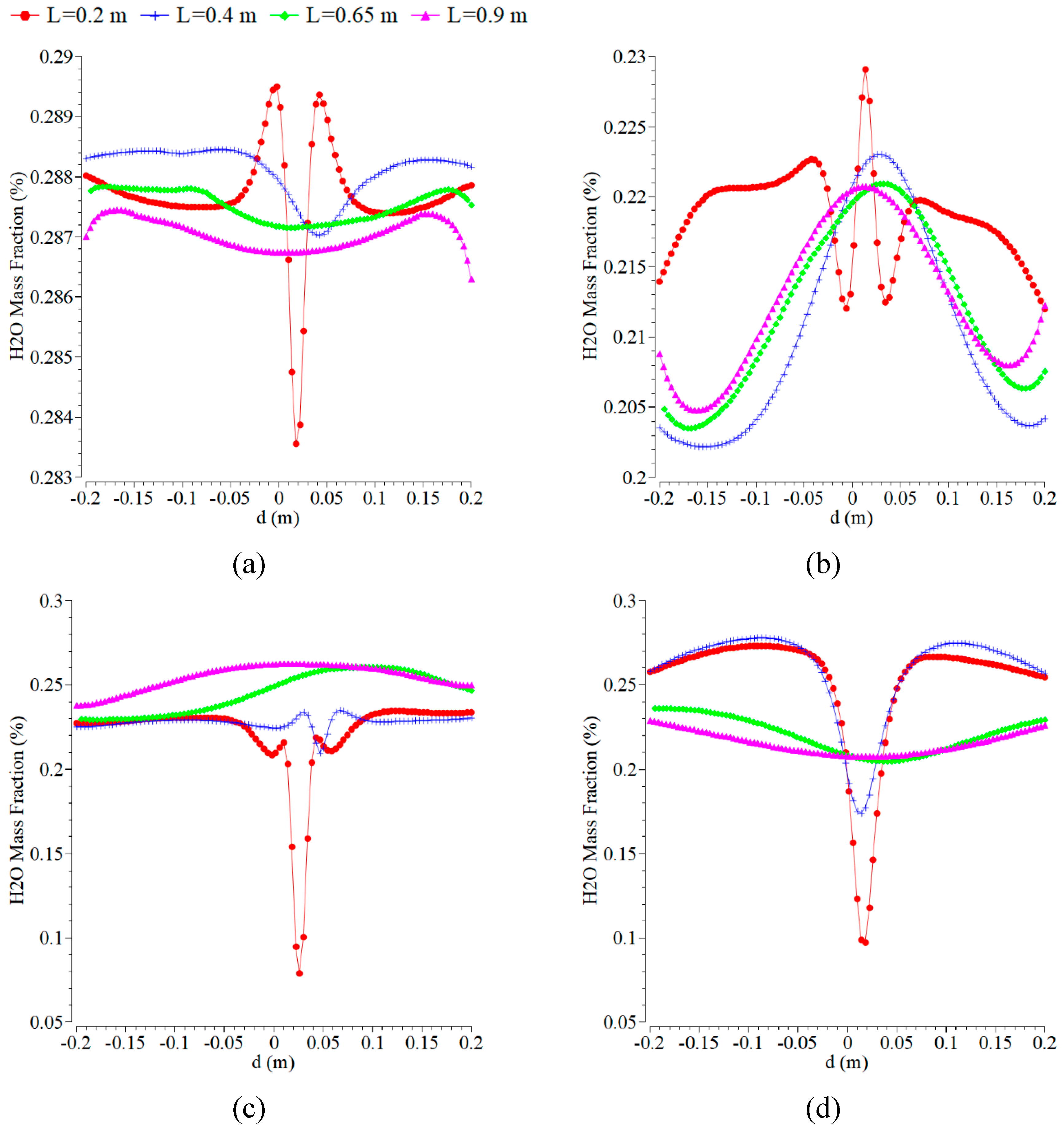
Figure 4.
Contours of radial velocity at the velocity magnitude of the air inlet of 0.5 m/s and the fuel inlets of: (a) 0.01 m/s, Tin= 700 K; (b) 0.01 m/s, Tin= 300 K; and (c) 0.1 m/s, Tin= 300 K.
Figure 4.
Contours of radial velocity at the velocity magnitude of the air inlet of 0.5 m/s and the fuel inlets of: (a) 0.01 m/s, Tin= 700 K; (b) 0.01 m/s, Tin= 300 K; and (c) 0.1 m/s, Tin= 300 K.
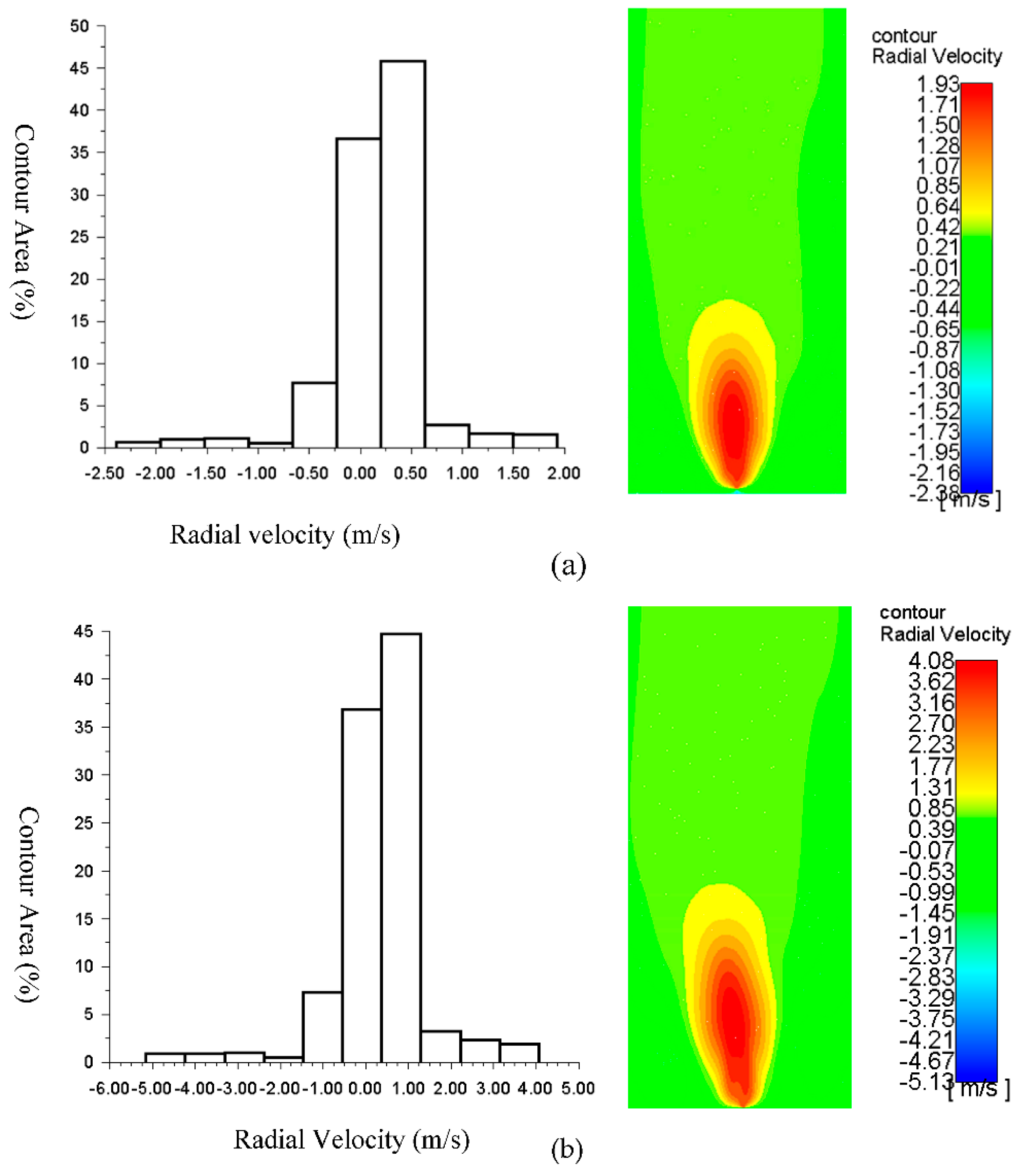
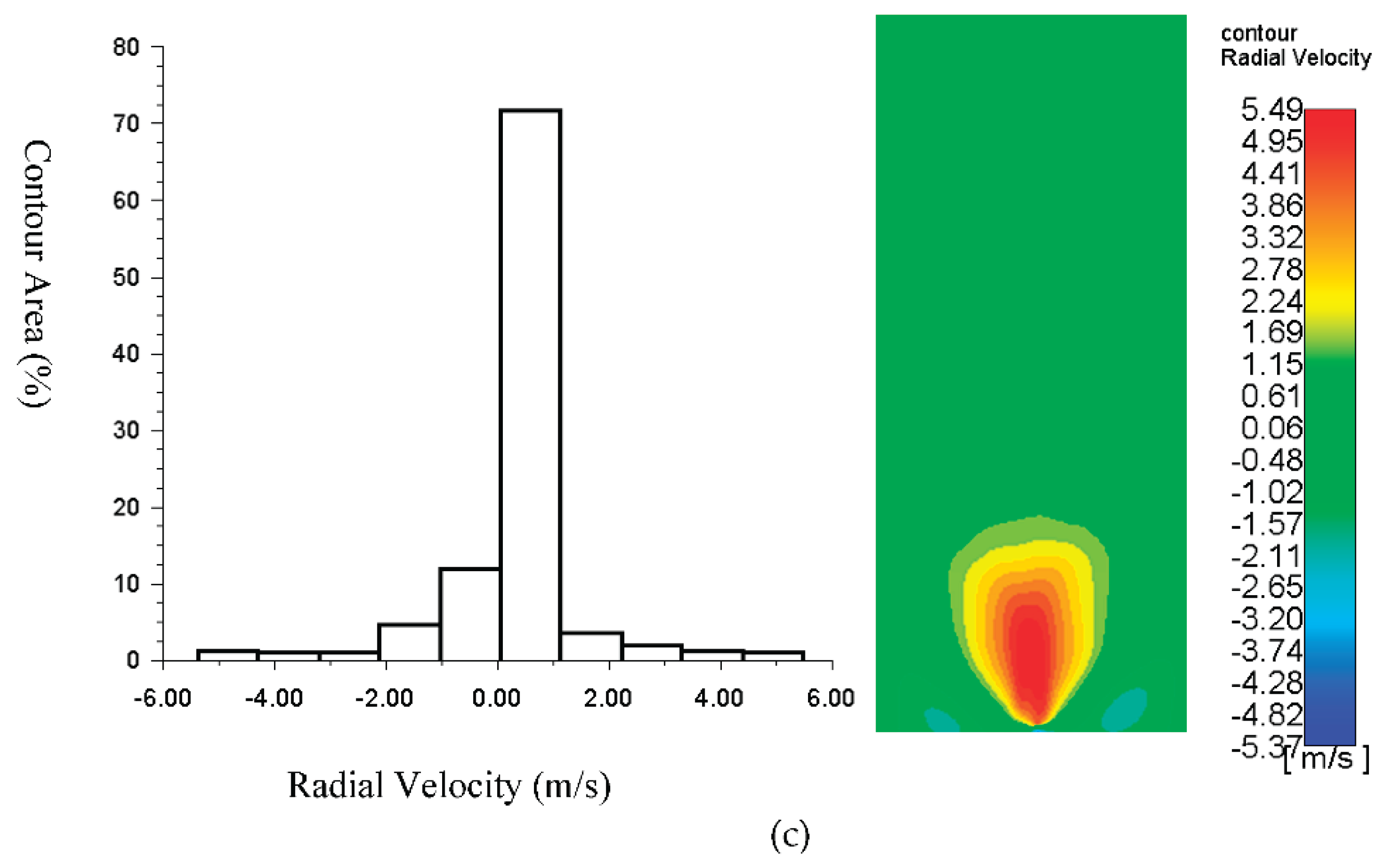
Figure 5.
The mass fraction contours of CO, CO2, and HCO at the axial positions of 0.2, 0.4, 0.65, and 0.9 m with the velocity magnitude of the air inlet of 0.5 m/s and varying the fuel inlets: (a) 0.05 m/s; (b) 0.1 m/s; (c) 0.3 m/s; (d) 1.5 m/s; (e) 0.05 m/s; (f) 0.1 m/s; (g) 0.3 m/s; (h) 1.5 m/s; (i) 0.05 m/s; (j) 0.1 m/s; (k) 0.3 m/s; and (l) 1.5 m/s.

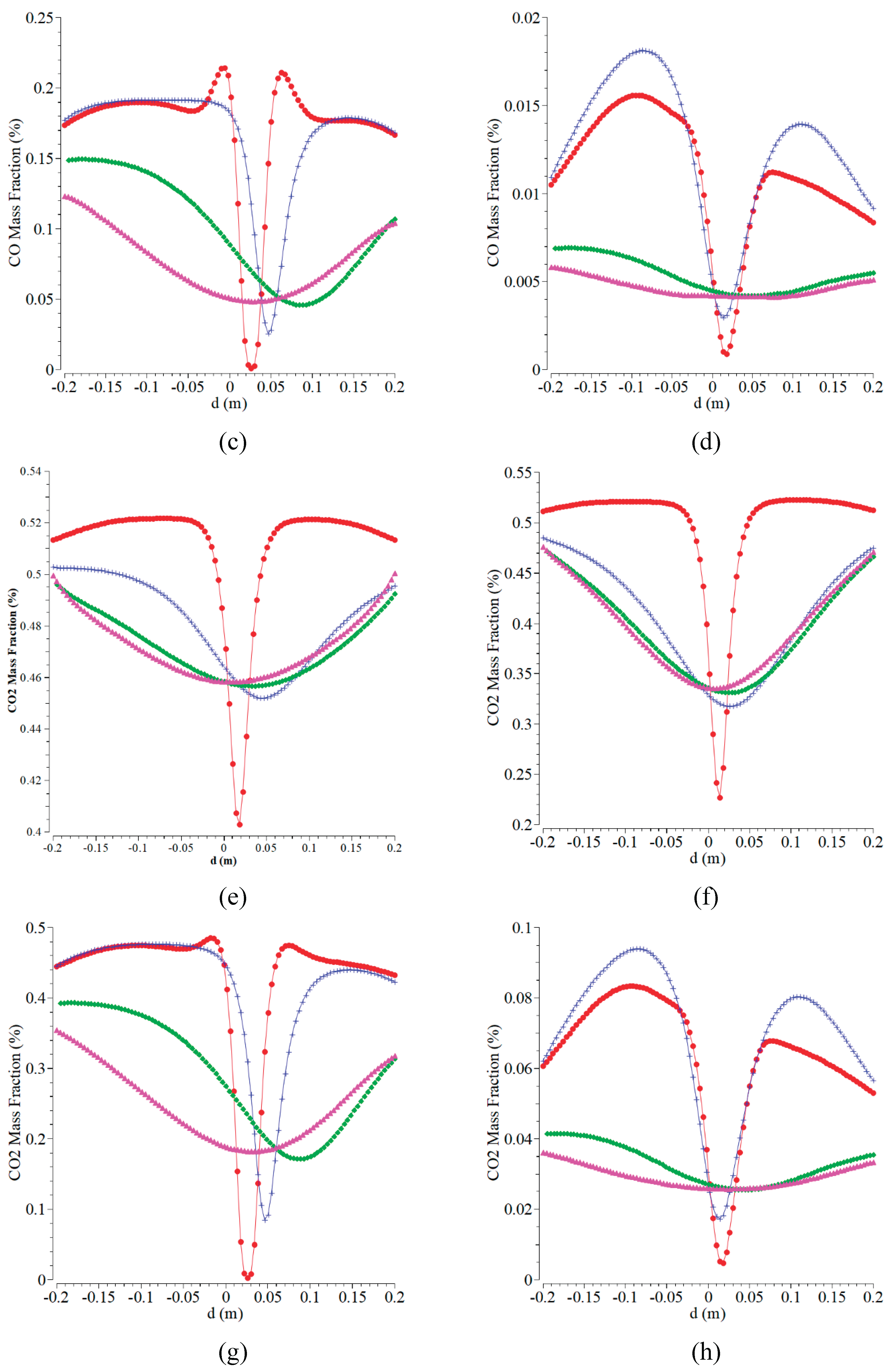

Figure 6.
The temperature distribution at the radial positions of 0, 0.025, -0.1, 0.1, and 0.2 m with the velocity magnitudes of the air inlet of 0.5 m/s and the fuel inlet of 0.01 m/s. The inlet temperatures of air and fuel are A. 500 K, B. 700 K, C. 900 K, D. 1500 K.
Figure 6.
The temperature distribution at the radial positions of 0, 0.025, -0.1, 0.1, and 0.2 m with the velocity magnitudes of the air inlet of 0.5 m/s and the fuel inlet of 0.01 m/s. The inlet temperatures of air and fuel are A. 500 K, B. 700 K, C. 900 K, D. 1500 K.
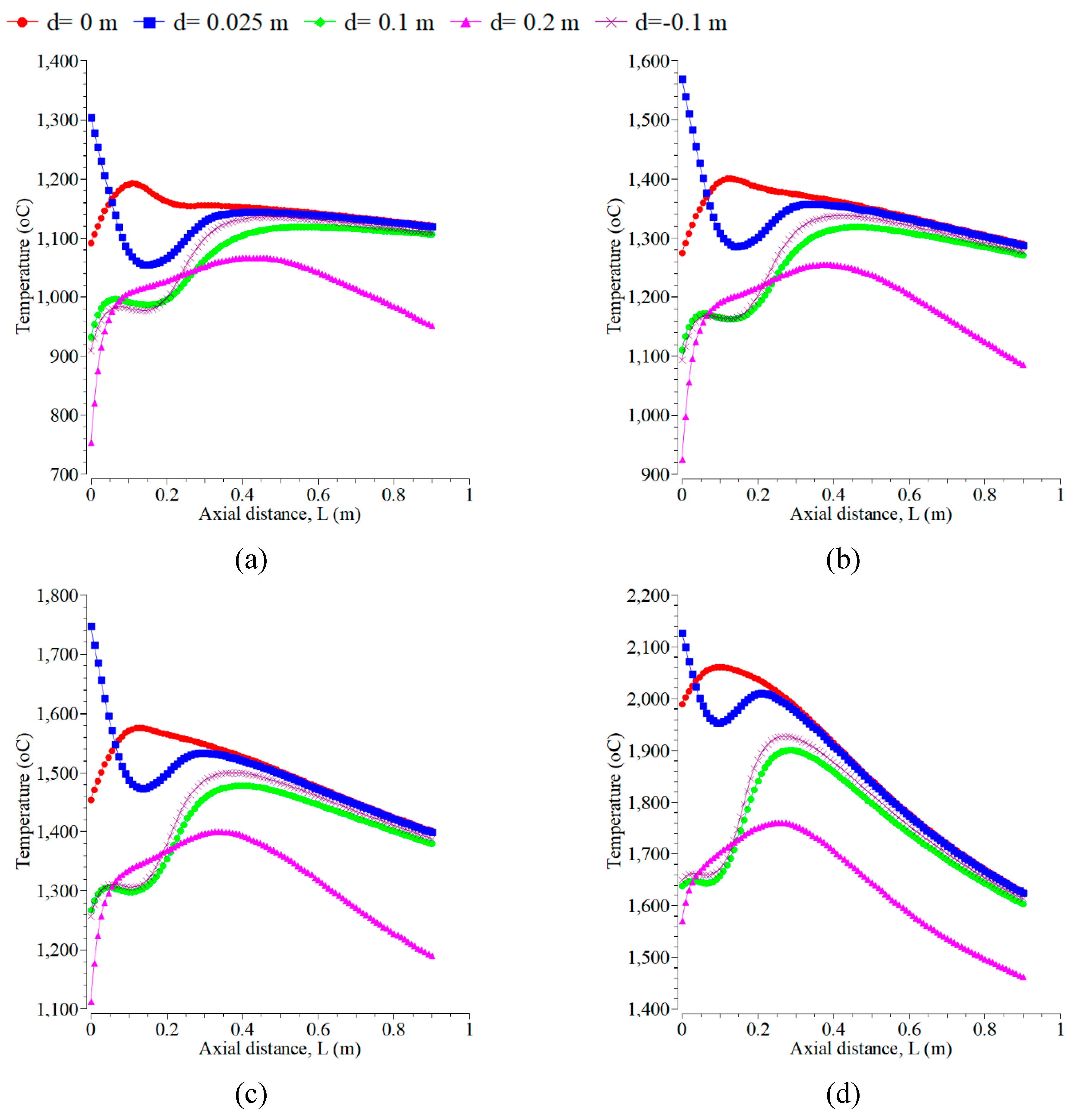
Figure 7.
CO mass fractions at the radial positions of 0, 0.025, -0.1, 0.1, and 0.2 m with the velocity magnitudes of the air inlet of 0.5 m/s and the fuel inlet of 0.01 m/s. The inlet temperatures of air and fuel are: (a) 500 K; (b) 700 K; (c) 900 K; (d) 1500 K.
Figure 7.
CO mass fractions at the radial positions of 0, 0.025, -0.1, 0.1, and 0.2 m with the velocity magnitudes of the air inlet of 0.5 m/s and the fuel inlet of 0.01 m/s. The inlet temperatures of air and fuel are: (a) 500 K; (b) 700 K; (c) 900 K; (d) 1500 K.
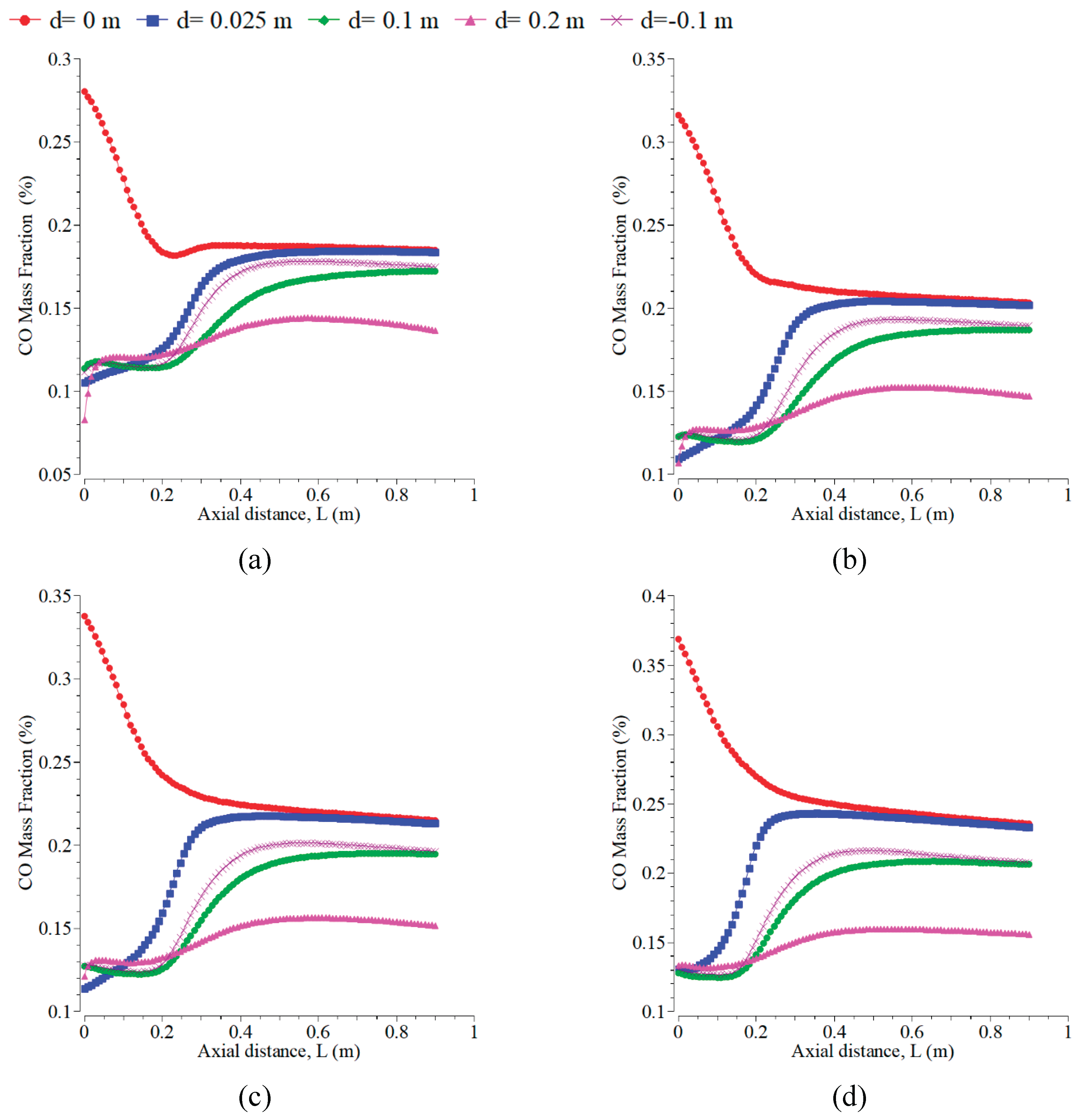
Figure 8.
CO2 mass fraction with the velocity magnitudes of the air inlet of 0.5 m/s and the fuel inlet of 0.01 m/s. The radial positions are: (a) 0 m; (b) 0.025 m; (c) 0.1 m; and (d) -0.1 m.
Figure 8.
CO2 mass fraction with the velocity magnitudes of the air inlet of 0.5 m/s and the fuel inlet of 0.01 m/s. The radial positions are: (a) 0 m; (b) 0.025 m; (c) 0.1 m; and (d) -0.1 m.
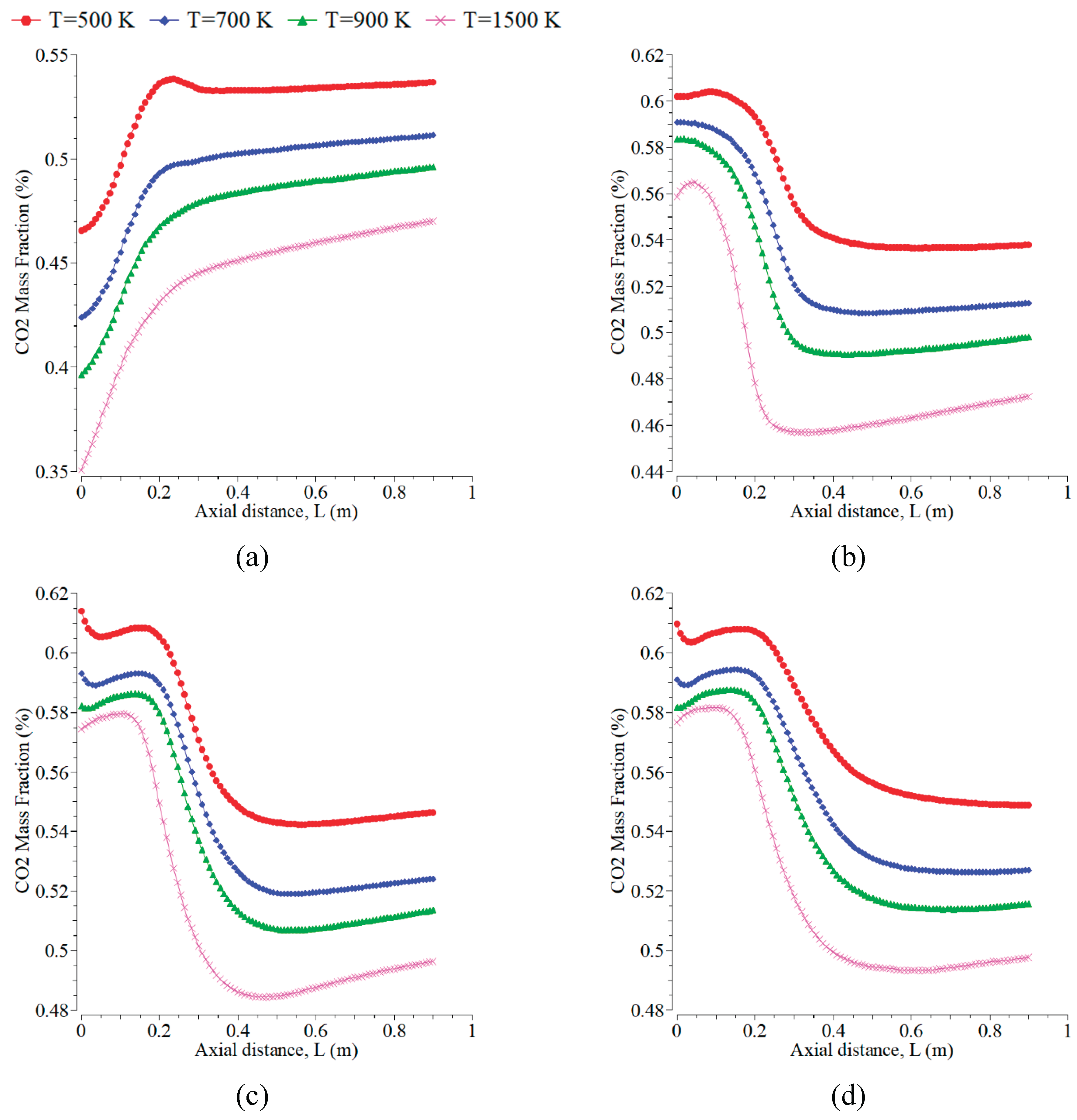
Figure 9.
Air and fuel contours of H2O mass fraction at the velocity magnitude of the air inlet of 0.5 m/s and the fuel inlet of 0.01 m/s with various inlet temperatures of air and fuel.
Figure 9.
Air and fuel contours of H2O mass fraction at the velocity magnitude of the air inlet of 0.5 m/s and the fuel inlet of 0.01 m/s with various inlet temperatures of air and fuel.
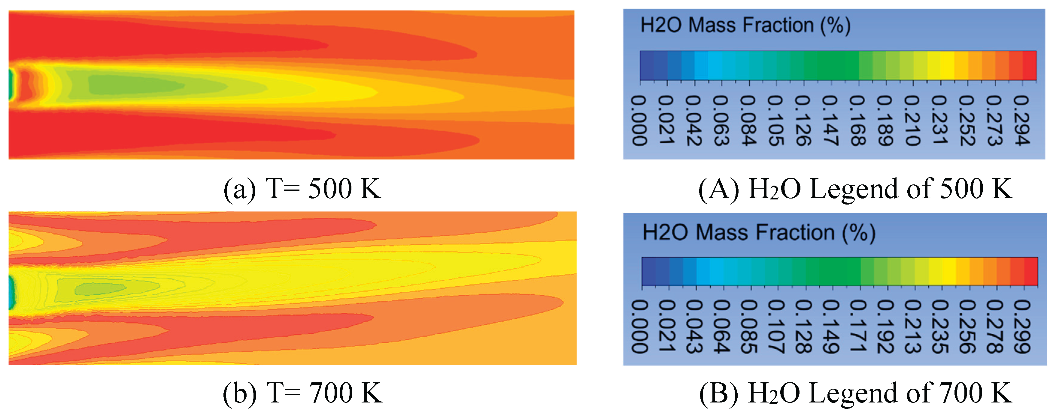
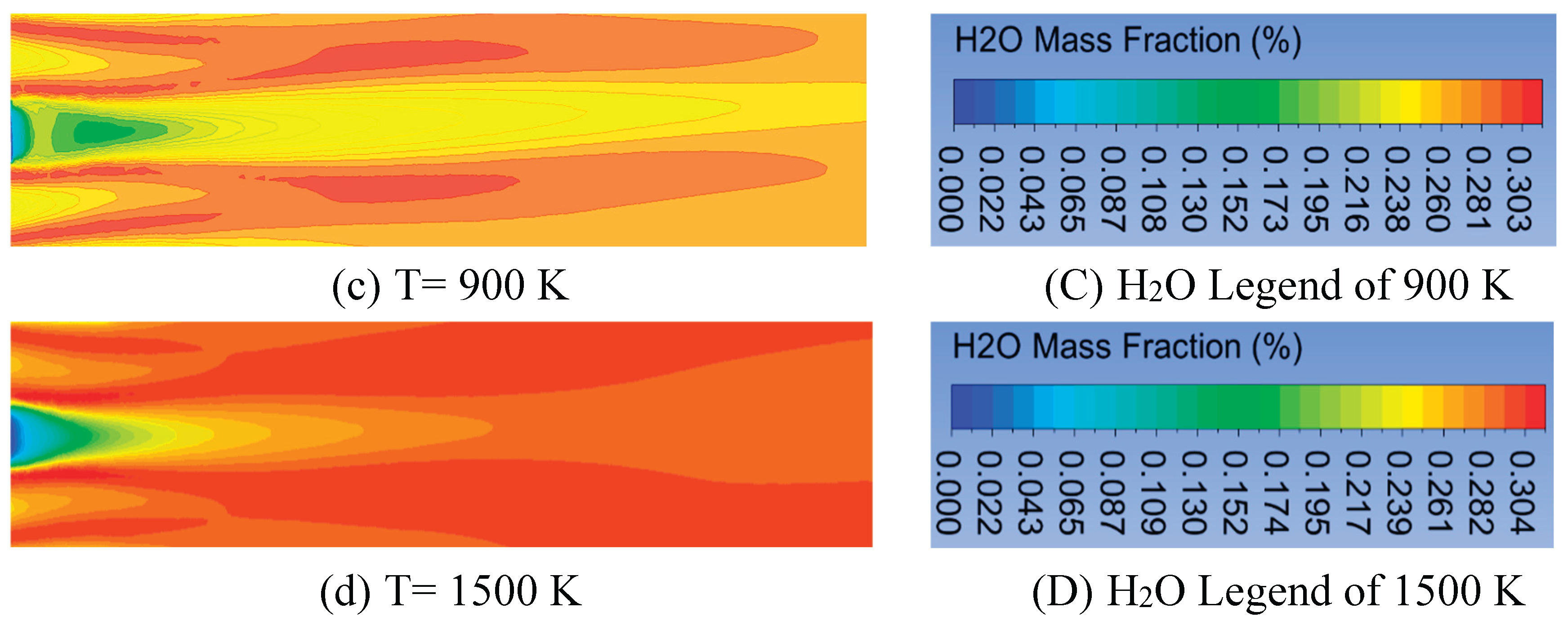
Figure 10.
Axial temperature profile at the radial positions of 0, 0.025, -0.1, 0.1, and 0.2 m with the velocity magnitude of the air inlet of 0.5 m/s and the fuel inlet of 0.01 m/s, using various oxygen mass fractions: (a) O2= 0.5%, N2= 0.5%; (b) O2= 0.5%, N2= 0.2%, CO2= 0.1%, CO= 0.1%, and H2O= 0.1%; (c) O2= 0.7%, CO2= 0.1%, CO= 0.1%, and H2O= 0.1%; (d) O2= 0.8%, CO2= 0.1%, and H2O= 0.1%.
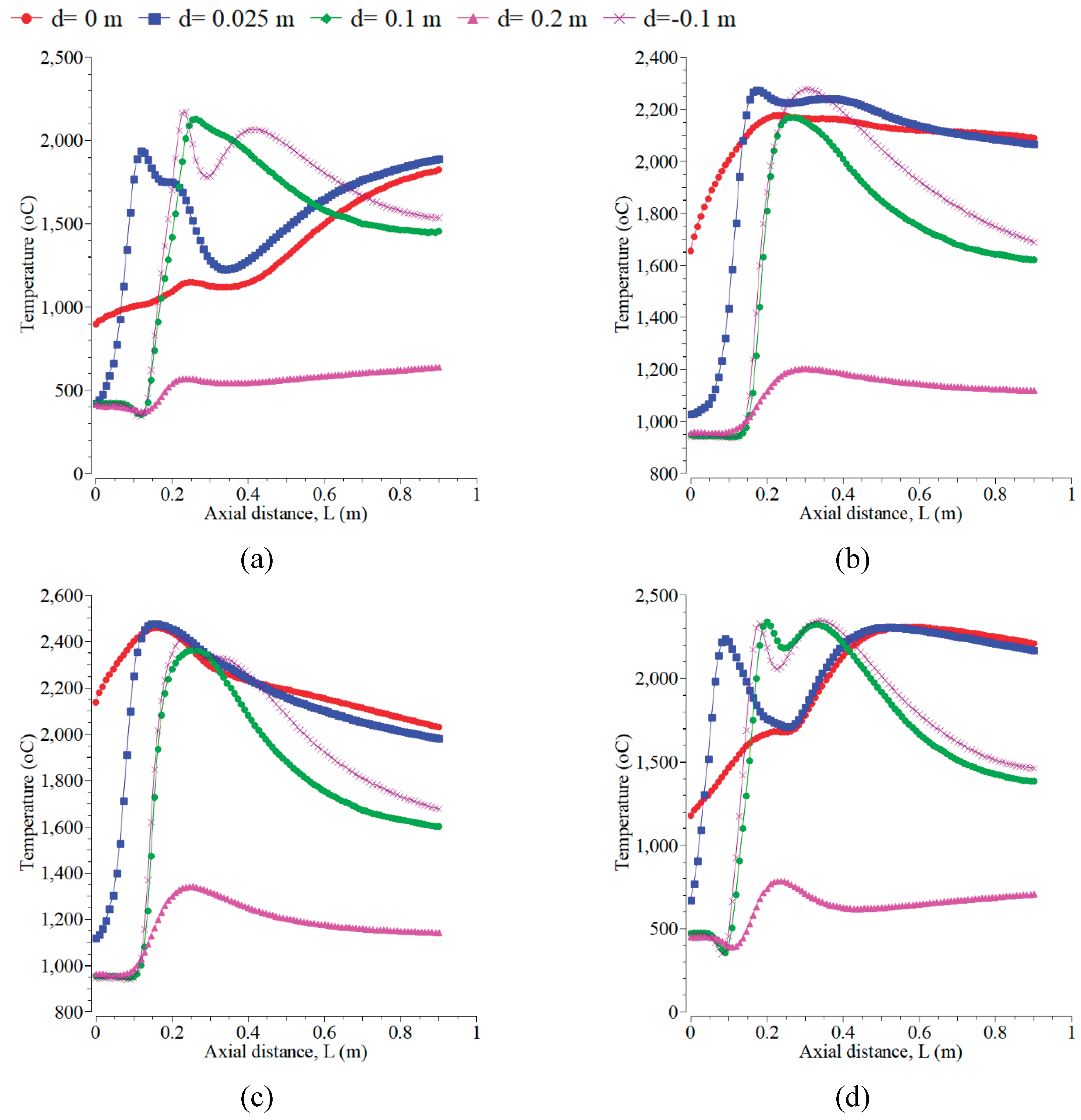
Figure 11.
The mass fractions of CO2, CO, and H2O at the radial positions of 0, 0.025, -0.1, 0.1, and 0.2 m with the velocity magnitudes of the air inlet of 0.5 m/s and the fuel inlet of 0.01 m/s, using various oxygen concentrations: (a; e; i) O2= 0.5%, N2= 0.5%; (b; f; j) O2= 0.5%, N2= 0.2%, CO2= 0.1%, CO= 0.1%, and H2O= 0.1%; (c; g; k). O2= 0.7%, CO2= 0.1%, CO= 0.1%, and H2O= 0.1%; (d; h; l). O2= 0.8%, CO2= 0.1%, and H2O= 0.1%.
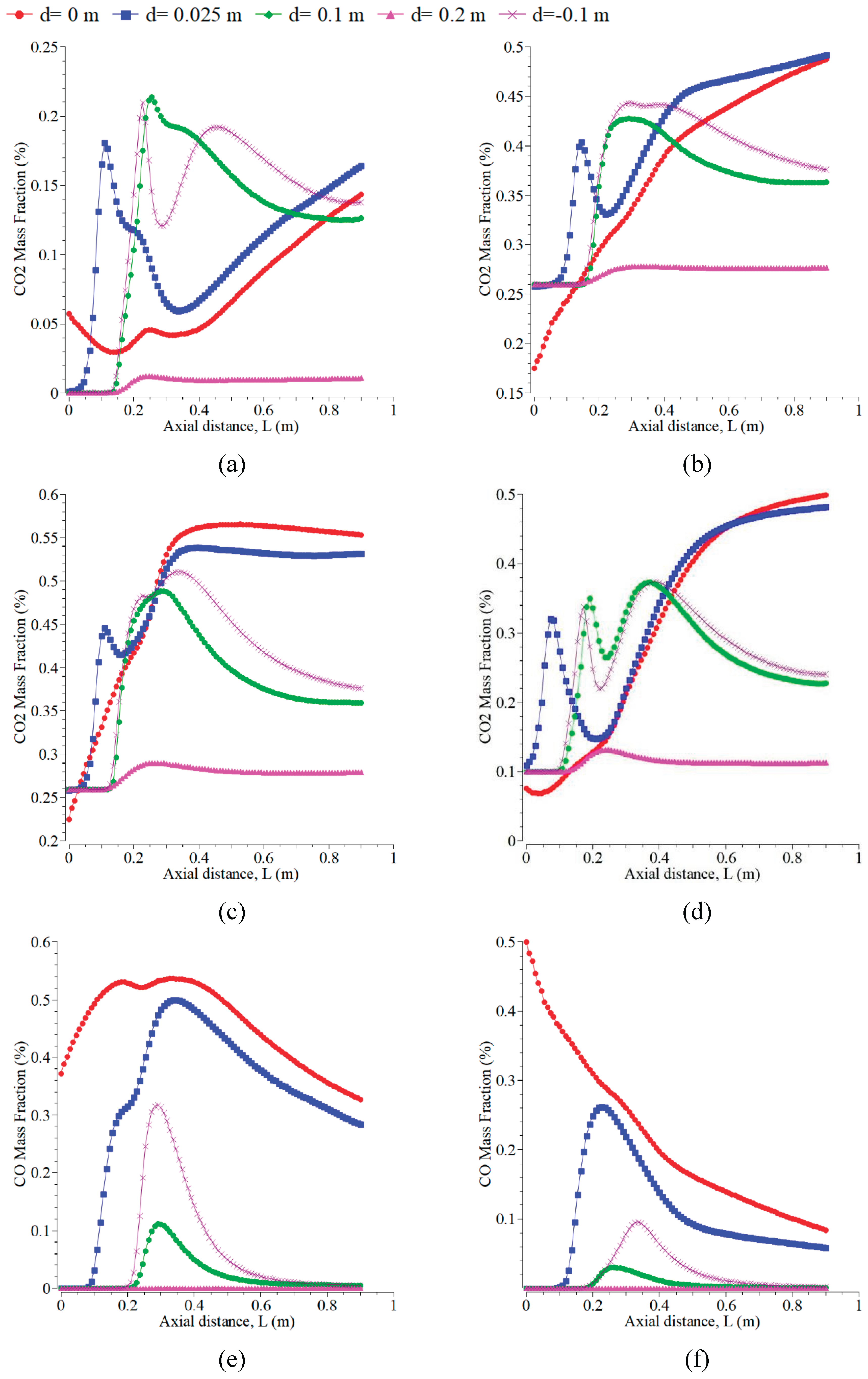
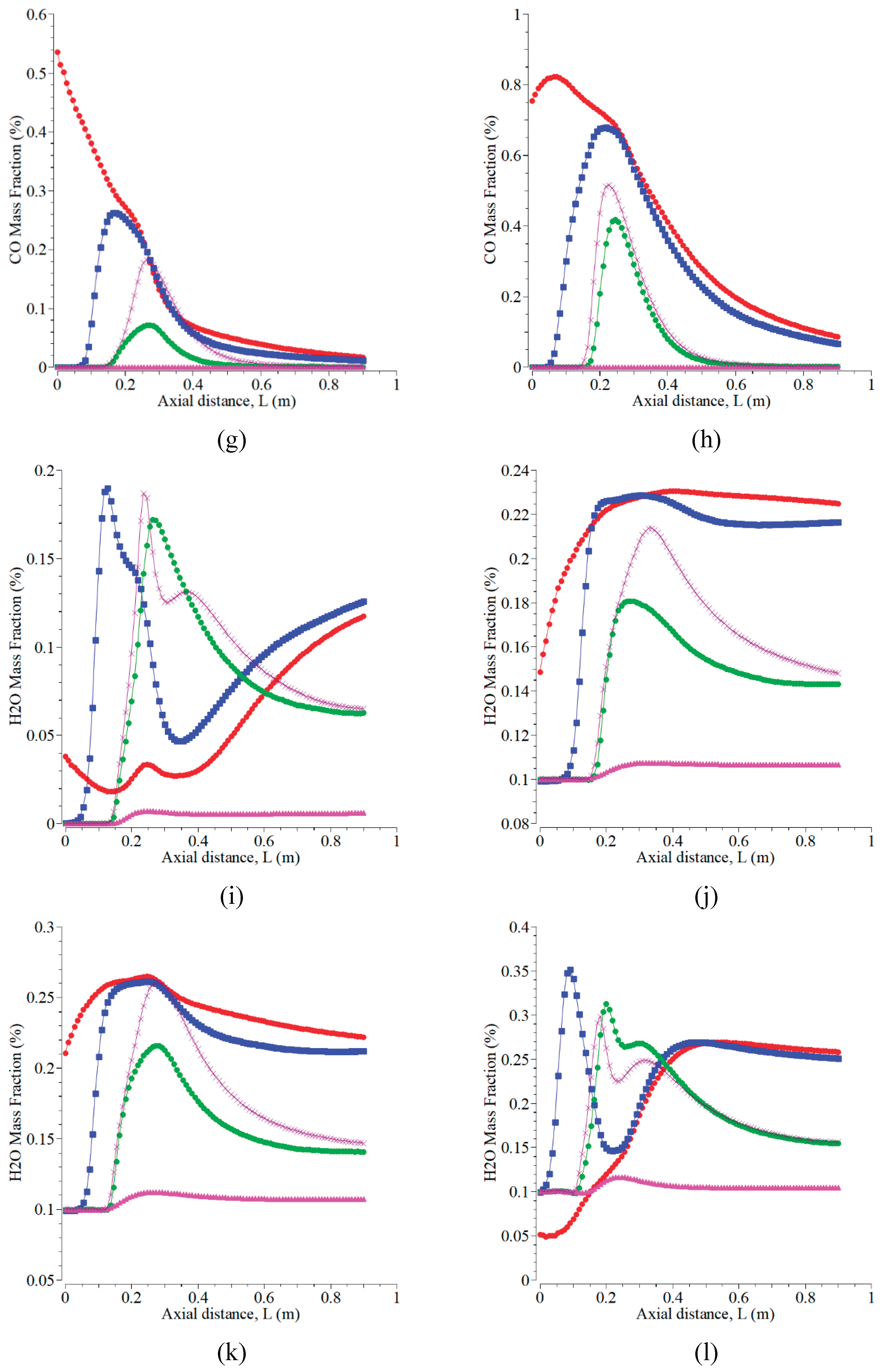
Figure 12.
Temperature contour at the velocity magnitudes of the air inlet of 0.5 m/s and the fuel inlet of 0.01 m/s with various concentrations of oxygen: (a) O2= 0.5%, N2= 0.5%; (b) O2= 0.5%, N2= 0.2%, CO2= 0.1%, CO= 0.1%, and H2O= 0.1%; (c) O2= 0.7%, CO2= 0.1%, CO= 0.1%, and H2O= 0.1%; (d) O2= 0.8%, CO2= 0.1%, and H2O= 0.1%.
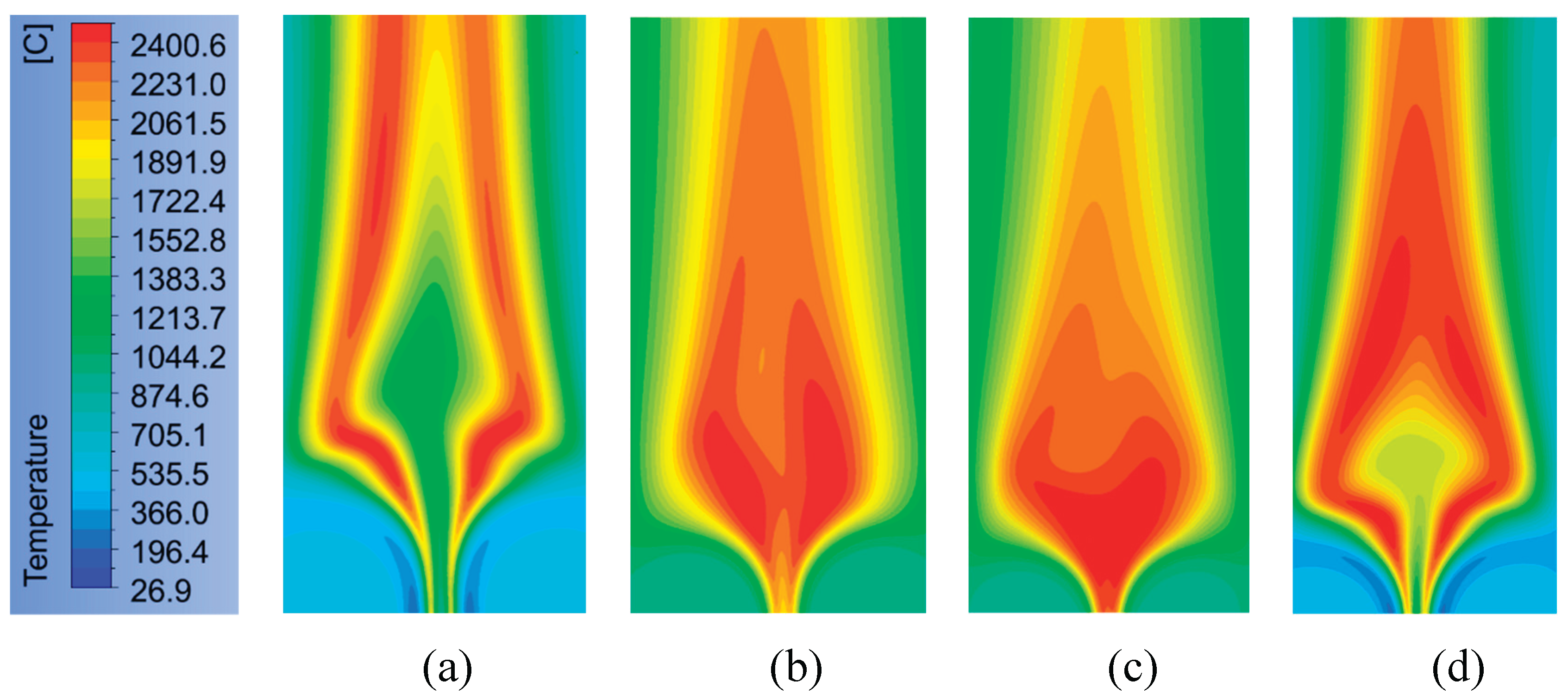

Table 1.
Boundary conditions of inlet fuel, inlet air, wall, and pressure.
| Boundary conditions | Parameters | Values |
| Inlet air | ||
| Momentum | Velocity (m/s) | 0.5 |
| Hydraulic diameter (m) | 0.03 | |
| Turbulent intensity (%) | 10 | |
| Thermal | Temperature (K) | 300 |
| Species | Oxygen (mass fraction) | 0.21 |
| Inlet fuel | ||
| Momentum | Velocities (m/s) | 0.01, 0.03, 0.05, 0.075, 0.1, 0.3, 1, 5 and 10 |
| Hydraulic diameter (m) | 0.02 | |
| Turbulent intensity (%) | 10 | |
| Thermal | Temperature (K) | 300 |
| Species | Kerosene (mass fraction) | 1 |
| Walls | Wall slip | 0 |
| Material | Steel | |
| Thermal condition | Mixed | |
| Heat transfer convection (W/m2.K) | 0 | |
| Outlet pressure | Gauge pressure | 0 |
| Hydraulic diameter (m) | 0.5 | |
| Turbulent intensity (%) | 10 |
Table 2.
Setup of simulation.
| Models | Parameters |
| Viscous model | K-e Standard |
| Radiation model | P1 |
| Combustion model | Diffusion combustion flame |
| Mixture properties | Kerosene (C12H23)-air |
| Turbulence chemistry interaction | Eddy dissipation model (EDM) |
| Reaction | Volumetric |
| NOx | Thermal and prompt NOx |
Disclaimer/Publisher’s Note: The statements, opinions and data contained in all publications are solely those of the individual author(s) and contributor(s) and not of MDPI and/or the editor(s). MDPI and/or the editor(s) disclaim responsibility for any injury to people or property resulting from any ideas, methods, instructions or products referred to in the content. |
© 2025 by the authors. Licensee MDPI, Basel, Switzerland. This article is an open access article distributed under the terms and conditions of the Creative Commons Attribution (CC BY) license (https://creativecommons.org/licenses/by/4.0/).
Copyright: This open access article is published under a Creative Commons CC BY 4.0 license, which permit the free download, distribution, and reuse, provided that the author and preprint are cited in any reuse.


