Submitted:
24 July 2025
Posted:
25 July 2025
You are already at the latest version
Abstract
This study is a novel optical approach that employs light-induced phosphorescence from thermographic phosphor thin films. The heat fluxes and wall temperatures of almost one-dimensional flat premixed flames that primarily strike upward against a horizontally oriented, water-cooled, circular flat plate are examined using this method. To evaluate the heat flow rate from the flame, chromium-doped alumina (Cr: Al2O3) ruby was applied to both sides of the plate's core, which is an alumina ceramic substrate. The substrate was excited on both sides by a green light-emitting diode (LED) array, and temperature measurements were taken on either side. When the fuel–air mixture flows at lower velocities (0.05–0.5 m/s), a matrix-style flat burner enclosed in a water-cooled jacket produces a laminar, one-dimensional flame. Nozzle burner is better suited for higher fuel-air mixture velocities (0.6-1.2 m/s). A hollow, water-streamed disk with an outside diameter of 200 mm and a thickness of 30 mm comprises the heat receiver. A brass ring encircles the ceramic plate on the flame side, while the top is sealed with a translucent acrylic glass cover. The acrylic glass maintains exceptional transparency across the phosphorescence and excitation wavelength ranges and remains dimensionally stable at temperatures relevant to the experiment (up to about 120 °C on the water-cooled, pressurized side). On the heated side of the ceramic plate, the temperature remained relatively low (under 500 K) due to the direct contact between the plate’s backside and pressurized cooling water at approximately 3 bar.The receiver disk features 12 mm diameter cooling-water channels located on its opposing faces. The ceramic plate, which is made of aluminium oxide (Al2O3), is 80 mm in diameter and 6 mm thick. Ruby is used as a phosphor on both sides of the plate. A green light-emitting diode (LED) array with a peak wavelength of 525 nm and an average output power of 2.4 W was used to light the plates. The signal of phosphorescence from each side of the plate was detected with the aid of two photomultiplier (PM) tubes. Before being transferred to a PC, the signal was averaged over 128 pulses using a digital oscilloscope. A rapid pulse generator provided the driving signal for the green LED. Data concerning the heat flux rate were derived from these investigations. The findings of the model were compared with those of the experiments.
Keywords:
Heat flux
; Thermographic Phosphors
; ruby
; light-emitting diode (LED)
; laminar flame
; Stagnation point
1. Introduction
One crucial thermodynamic characteristic that characterizes chemical, biological, and physical processes is temperature. A lot of work was invested in getting accurate temperature readings for a variety of uses. Accurate temperature measurement is essential for a deeper knowledge of heat transport mechanisms in combustion and related applications. Measuring the surface temperature is particularly important when figuring out how much heat solid walls absorb from flames. Temperature is frequently measured employing thermocouples or optical pyrometry. However, these methods possess certain drawbacks.
It is challenging to produce the very good thermal contact required by thermocouples, particularly when measuring the temperatures of moving elements (such as those found in machines). Pyrometry might be an option in these situations, but it requires information about the monitored surface’s emissivity, which is again challenging to do, particularly in processes where the emissivity changes over time. These disadvantages are resolved by thermographic phosphors, which make them an excellent technique for measuring surface temperature and are accurate and practical for a range of thermal monitoring applications [1,2,3,4]. Phosphors are materials infused with small amounts of dopants that emit light when properly stimulated. Many different types of ceramic phosphors are easy to use, long-lasting, insoluble in water, and resistant to extreme physical and chemical conditions. Phosphors can be employed at temperatures ranging from 2000 °C to cryogenic levels [5].
In addition, the temperature measurement using thermographic phosphors was used in many applications such as heat fluxes from laminar flames to solid walls, measuring the temperatures of turbine blades and gas turbine combustors [6,7,8,9]. As heat is regularly delivered to surfaces as a result of the combustion enthalpy released by gas flames, significant convective heat transfer rates are observed in direct impinging jets.
Consequently, flame impingement heating is extensively employed in numerous industrial processes—such as glass shaping and metal melting. Generally speaking, the heat transfer from these jets is at least two-dimensional and is frequently explained as a function of the Reynolds number, Nusselt number, and dimensionless distance. The ratio of gas velocity to flame speed is generally not considered a significant parameter. On the other hand, this characteristic can be thoroughly examined using one-dimensional stagnation point geometries.
Because premixed stagnation flames exhibit an essentially one-dimensional structure, numerical modelling shows to be particularly advantageous, typically allowing for easier comparisons between the model and experimental findings. The study examined heat flux at the stagnation point of a one-dimensional, laminar premixed methane/air flame impinging onto a flat surface, maintained at a fixed burner-to-plate distance of 1.5 cm. The fundamental idea behind thermographic phosphors is widely known. The heat dependency of phosphorescence characteristics, covering features like intensity, line width, line position, and decay rate, is exploited by phosphor thermometry. The metric that is typically measured to ascertain the temperature is the phosphorescence decay period, sometimes referred to as lifetime. This method provides high accuracy and sensitivity.
This study investigates the heat flux of (almost) one-dimensional flames using phosphor thermometry.
For varying flow velocities, methane-air and methane-hydrogen-air flames are investigated at comparatively close distances between the burner and the surface. These experiments were conducted to determine the rate of heat flux. The outcomes of the experiments and the modelling were compared.
2. Theory
2.1. Phosphorescence
The term luminescence describes the phenomenon where a material takes in energy and then releases light.This is an occurrence that is not the same as blackbody radiation, incandescence, or other phenomena that make materials emit light when subjected to high temperatures. Phosphorescence refers to a form of luminescence characterized by an extended duration, typically ranging from 10-3 to 10 3 seconds. A phosphor refers to a delicate white or subtly colored powder that is specifically formulated to fluoresce effectively. The duration of an excited inorganic phosphor’s phosphorescence following stimulation with a light pulse is the basis for the temperature measurement technique. The lifespan depends on the temperature. A straightforward exponential function that accurately depicts the signal structure is typically fitted to determine the decay time. In this instance:
where t is the time since the excitation source stopped, I is the phosphorescence light intensity, I0 is the initial phosphorescence light intensity at time t = 0, and τ is the phosphorescence decay period. Chromium-doped aluminium oxide (ruby), a well-known phosphor, was applied to both sides of a flat alumina ceramic plate used as the stagnation surface in this investigation (chromium concentration = 1.1%). Both sides of the ceramic plate’s phosphorescence lifetime’s temperature dependence were ascertained. Although Pflitsch et al. [10,11] demonstrated that pure rubies decay mono-exponentially. The plate exhibited temperature-dependent phosphorescence, resulting in slight variations from a decay that is mono-exponential. Brübach et al. [12] developed a method to deal with this issue.
2.2. Heat Flux Analysis
To determine the rate of local heat flux at the plate’s center, it is necessary to monitor temperatures from both sides simultaneously, where a one-dimensional stagnation flow can be maintained. This was additionally accomplished by applying phosphorescence thermometry to the water-cooled rear surface of the ceramic plate. The heat flux can then be ascertained using the computed temperature difference:
= heat flux; k = thermal conductivity, ΔT = temperature difference across the plate, = thickness of the plate, is the heat flow rate, and A is the area of the cross section. Since contributions from greater radial distances do not interfere with the current measurements, this experimental method is far more appropriate for determining the local heat flux rate than monitoring the cooling water’s energy balance. Additionally, the heat flux rate would need to be calculated by dividing the energy balance’s heat flow rate by an area. However, there are various ways to choose the area’s size, which could lead to unclear results. One crucial boundary condition for the flame modelling is the surface temperature on the ceramic plate’s flame side.
3. The Experimental Setup
This experiment was configured to approximate a one-dimensional stagnation-point geometry. Figure 1 shows a schematic diagram of the experimental setup. The two main structural components of the experimental setup are the burner, which generates heat, and the heat receiver, which absorbs heat. For lower fuel-air mixture velocities (0.05–0.5 m/s), a matrix flat burner encircled by a water-cooled jacket was employed to produce a laminar one-dimensional flame.
A nozzle burner is better suited for high flow rates. However, since the flame becomes stabilized within the tube, it is not suitable for lower velocities. A hollow, water-streamed disk with an outer diameter of 200 mm and a thickness of 30 mm comprises the heat receiver. A brass ring surrounds the ceramic plate on the flame-exposed side, and a translucent acrylic glass cover is placed over the top. The acrylic glass provides excellent transparency across the spectrum of phosphorescence and excitation wavelengths, remaining stable within the target temperature range—specifically under 120 °C on the pressurized, water-cooled side.
Because the backside was in direct contact with pressurized (≈3 bar) cooling water, the flame-facing side of the ceramic plate remained relatively cool (below 500 K). The cooling water drills are 12 mm in diameter and are positioned on opposing sides of the receiver disk. The ceramic plate, which has an 80 mm diameter and a 6 mm thickness of aluminum oxide (Al2O3), was coated with ruby phosphor on both faces. A high-performance green LED array (Opto Technologies Inc. model OTLH-0020-GN), featuring a peak wavelength of 525 nm and an average output of 2.4 W, was used to illuminate the plate. Two Hamamatsu H6780-03 photomultiplier tubes were employed to detect the phosphorescence signals from both sides of the ceramic plate. The phosphorescence signal was captured using a Tektronix TDS 2024 digital oscilloscope, averaged over 128 pulses, and subsequently transferred to a PC for analysis. The green LED was driven by a rapid pulse generator (Toellner TOE 7404).
3.1. Experimental Procedere
To achieve temperature consistency in the experimental setting, the cooling water flow was initiated fifteen minutes prior to the ignition of the fuel gas. For every trial, the cooling water flow was maintained at 20 l/h. After entering the burner, the premixed feed gases, air and methane are ignited. To determine whether the phosphorescence from both sides of the plate matched the calibration curve at the cooling water temperature, the lifespan of the gas combination was measured prior to ignition. Steady-state conditions, which were attained after the outlet water’s temperature stabilized, were used for the lifetime measurements with the burning flame. Both sides’ phosphorescence signals were concurrently captured, and the deviation was estimated by repeating each measurement three times. The average was used for additional analysis. At the minimum burner-to-plate gap (H = 15 mm), experiments were conducted at the stoichiometric composition of methane and air (Ф=1).
The tests were repeated at smaller velocities (0.05 and 0.08 m/s) as well as increasing the cold fuel mixture’s velocity from 0.1 m/s to 0.5 m/s in increments of 0.1The cooling water’s inlet and exit temperatures were measured using K-type thermocouples alongside PT100 platinum resistance thermometers. The ceramic plate’s upper surface temperature (i.e., on the cooling water side), and the flat burner’s surface temperature, respectively. Synthetic air (volume 21% O2 and 79% N2) was utilized to burn 99.99% pure methane. The gas flows were managed by three mass flow controllers (MKS devices). The aforementioned process was carried out again with 10% and 20% hydrogen added to the fuel mixture, and the outcomes were contrasted with those of a pure methane flame.
4. Results and Discussion
4.1. Surface Temperature Measurement
Surface temperatures on both sides of the plate were determined by analyzing the phosphorescence lifetime of ruby, which was excited by a green LED. At a distance of 1.5 cm, the surface temperature on both sides of the ceramic plate is measured using the porous matrix burner and plotted against the mass fluxes of the fuel-air combination for methane-air flames with 0%, 10%, and 20% hydrogen and a stoichiometric ratio of 1. Figure 2 shows that on both sides of the plate, the temperature is seen to rise.
Temperatures on the water side of the stoichiometric flame range from 300 to 350 K for the various flames. Temperatures of 320–385 K were detected on the flame side. Both the temperature differential and the heat flux rise as the mass flux of the fresh gases increases.
The measurements were made multiple times to lower the uncertainty and demonstrate their reproducibility.
The difference in temperature between the water-cooled and flame sides varies from 10 to 40 K. In modelling, the boundary condition was selected based on the flame side’s surface temperature. Surface temperatures of 350 or 390 K were selected for modelling since the precise surface temperature had little effect on the computed heat flux.
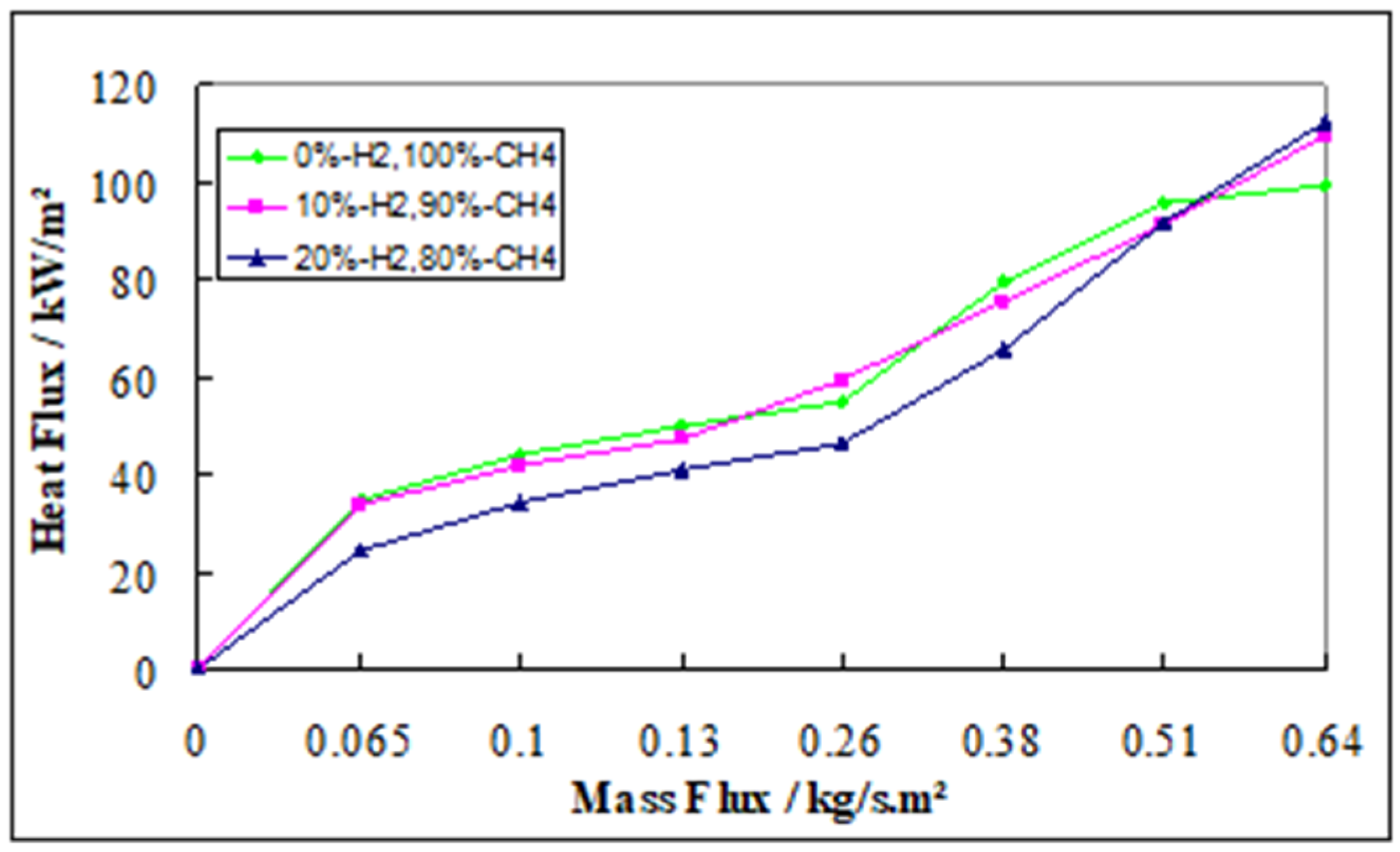
The evaluation of heat flux relies on these temperatures. Thermocouple measurements taken on the water-cooled side (not shown) read 2 – 10 K lower, highlighting the influence of thermal contact resistance. It can also be seen from the figure that on the addition of hydrogen to the flame, the surface temperatures on both faces of the plate rise. No conclusion can be made regarding the effect of the addition of hydrogen on the heat flux until the extent of the increase in temperature on both sides is separately evaluated. But by comparing the difference in temperature on both sides, the effect of hydrogen on the heat flux can be predicted. As can be seen in Figure 3. there is not much difference in heat flux on the addition of 10% hydrogen, but there is a significant reduction in the heat flux values when 20% hydrogen is added. This could be attributed to higher surface losses on the addition of more hydrogen.
4.2. Stagnation Heat Flux
The heat fluxes were calculated based on the recorded temperatures from both surfaces of the ceramic plate. The calculated experimental heat fluxes for the stoichiometric methane flame, both with and without hydrogen, are elegantly presented in Figure 3. The mean thermal conductivity of Al2O3 for both sides of the ceramic plate was used to calculate the experimental heat fluxes.
Since each experiment was conducted multiple times (3–5), the statistical errors for the variations were computed. This relative inaccuracy is greater in the lower temperature domain because there is a smaller temperature differential and a lesser temperature dependency of the ruby decay time, which rises with increasing temperature.
Heat fluxes measured experimentally range from 25 to 110 kW/m2. The slight variation between the mass flux and the heat flux mostly indicates that the enhanced gas flow causes a greater flow of high-enthalpy gases in a horizontal direction rather than a rise in the temperature gradient close to the surface. This would be considered a loss in heating.
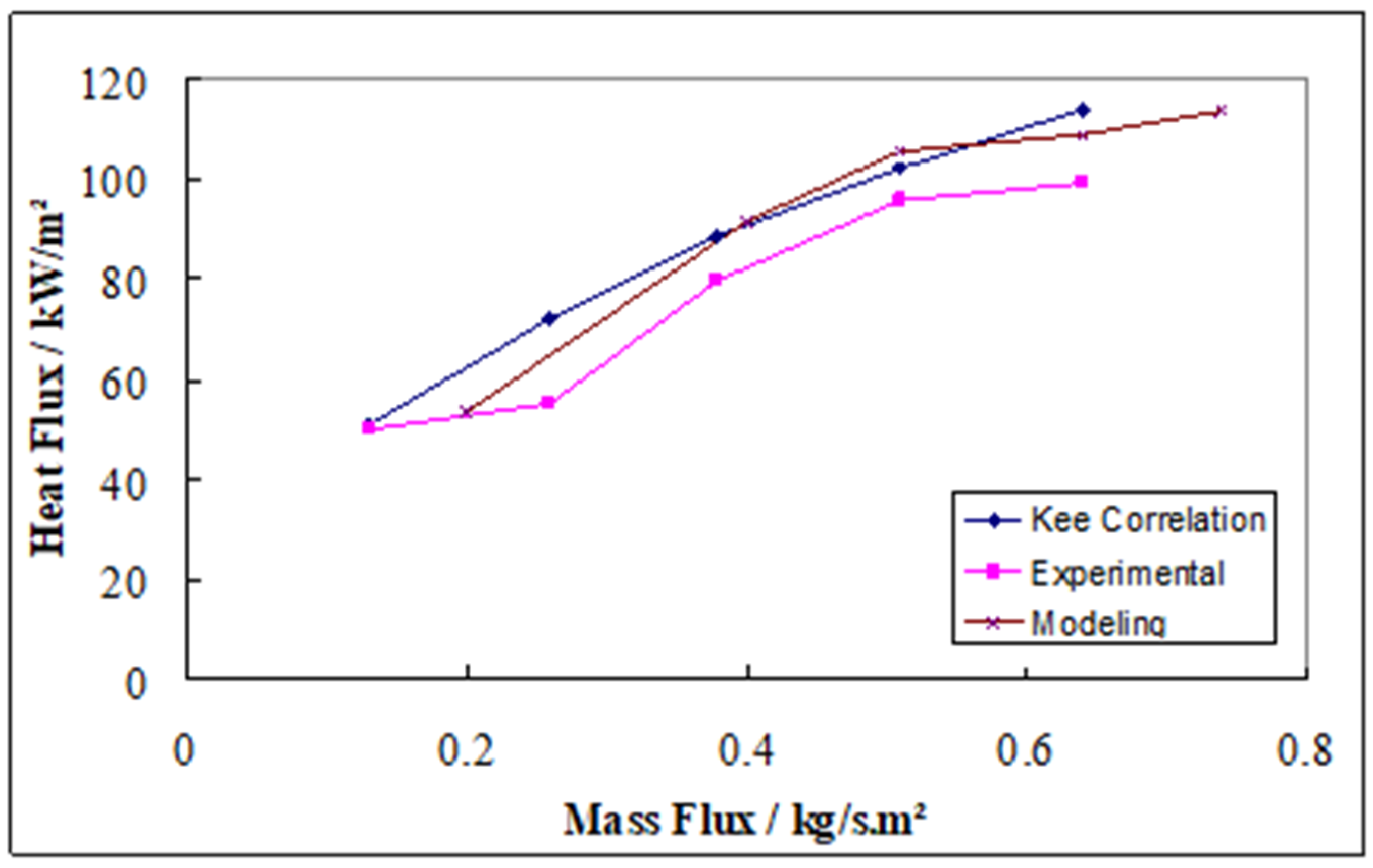
4.3. The Kee Correlation [13]
According to Fourier’s law,
Newton’s law of cooling:
Combining these two, we get:
For one-dimensional steady flow, the Nusselt number is given by:
Using these relations, a model was developed, and the results are compared below:
Figure 4.
Comparison of Heat flux results obtained from the experiment, Kee Correlation and model.
4.4. Uncertainty Analysis
Heat flux is calculated using the formula:
Here, ΔT represents the temperature difference between the flame-facing and water-cooled surfaces, L is the plate’s thickness, and k denotes the thermal conductivity of the ceramic material. So to calculate the uncertainty in heat flux, one must account for the errors in both ΔT and the thermal conductivity, k.
therefore,
When errors are irreversible. The inaccuracy in the heat flux, as determined by Kline and McClintok’s root-sum-square approach [14], is as follows:
All of the errors in this formula are relative. However, in this case, we ignore the error in Δx because the plate’s thickness is precisely known, and the only faults that affect the heat flux are those in ΔT and k. In this case, the standard deviation of the heat flux data was calculated and combined with the associated errors using the root-sum-square method. The relative errors for all the quantities, i.e., surface temperature for both sides, , thermal conductivity and finally heat flux, have been calculated. The heat fluxes for all three cases, along with their errors, have been plotted and are compared with the modelling results.
Figure 5.
Heat flux for pure methane-air flame for H=1.5 cm and Ф=1, and the modelled results.
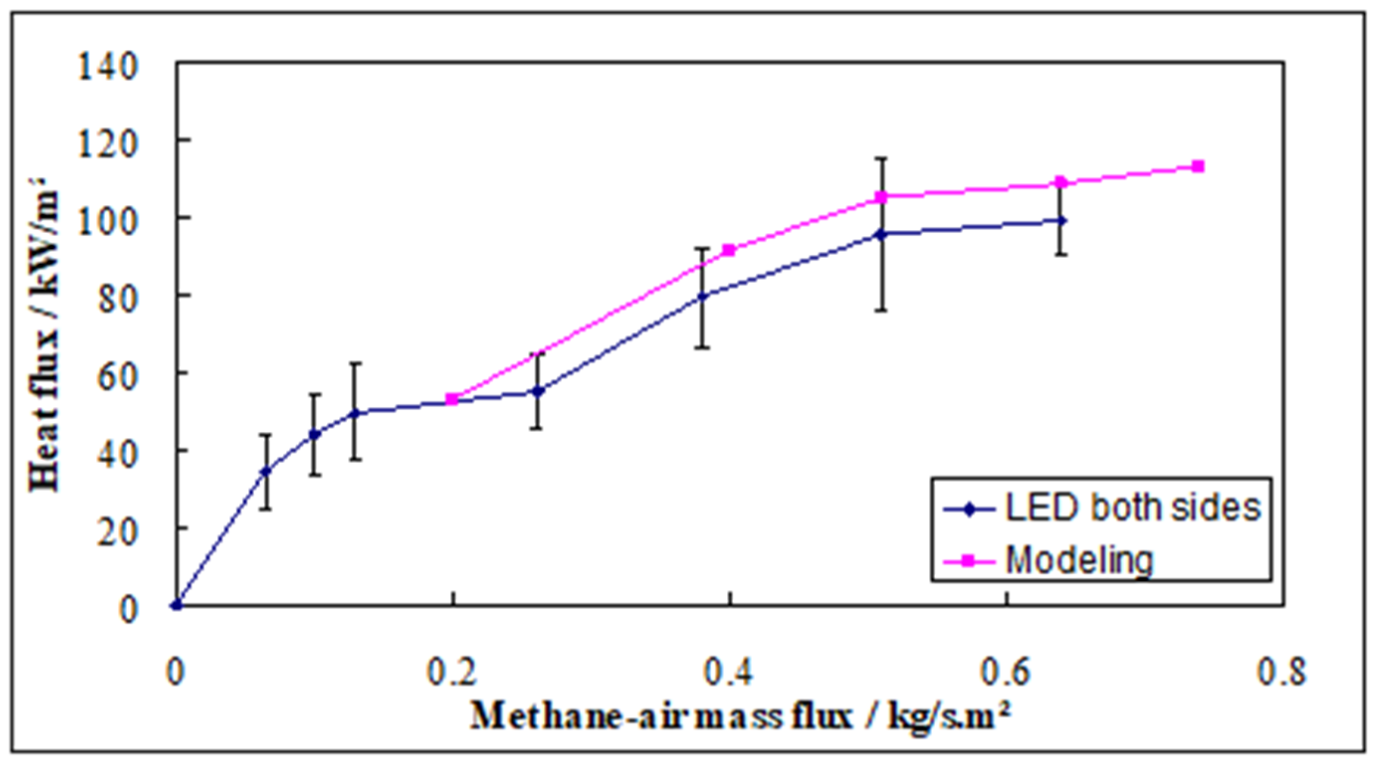
Figure 6.
Heat flux for 10%-hydrogen, 90%-methane-air flame for H=1.5 cm, Ф=1 and the modelled results.
Figure 6.
Heat flux for 10%-hydrogen, 90%-methane-air flame for H=1.5 cm, Ф=1 and the modelled results.
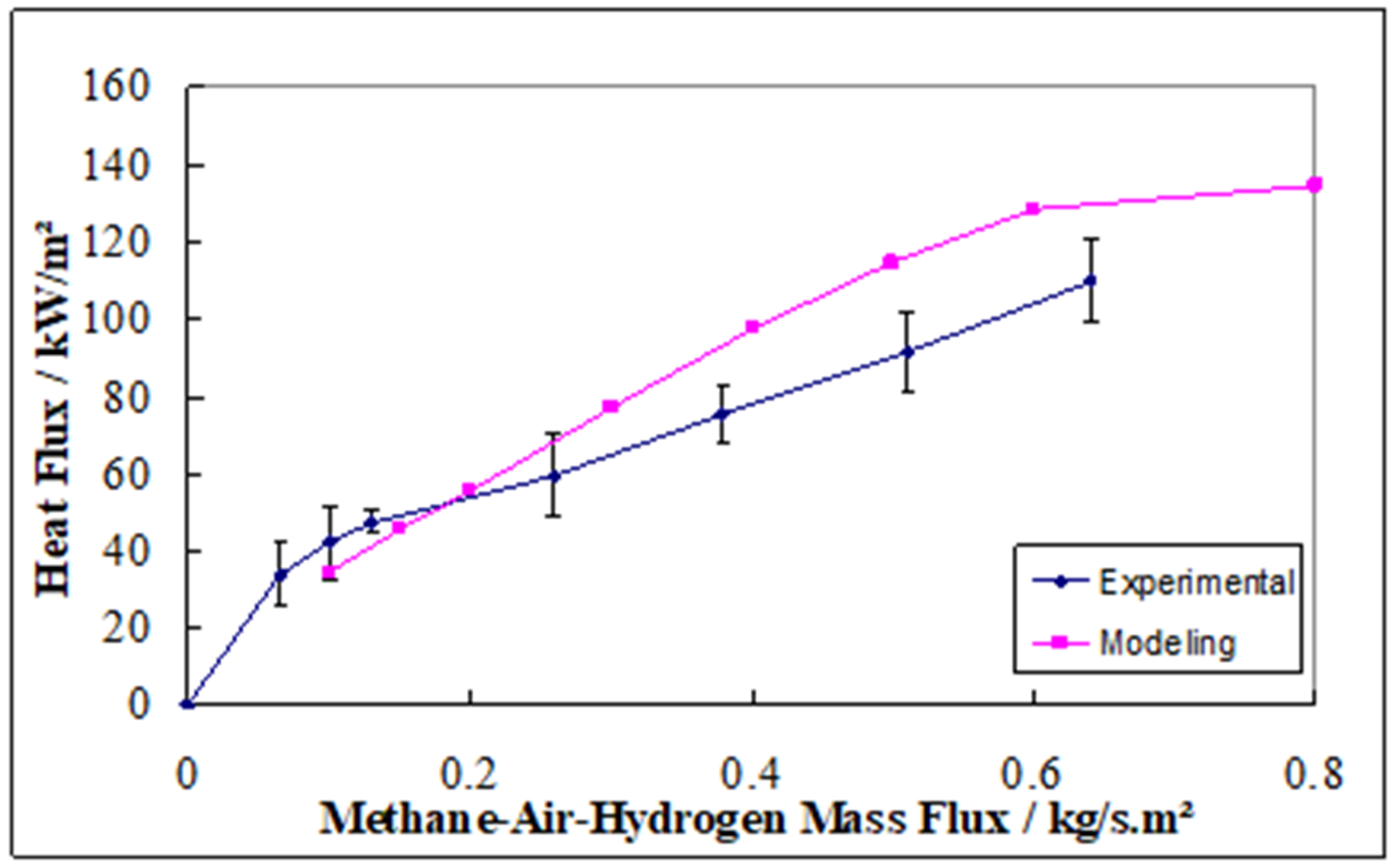
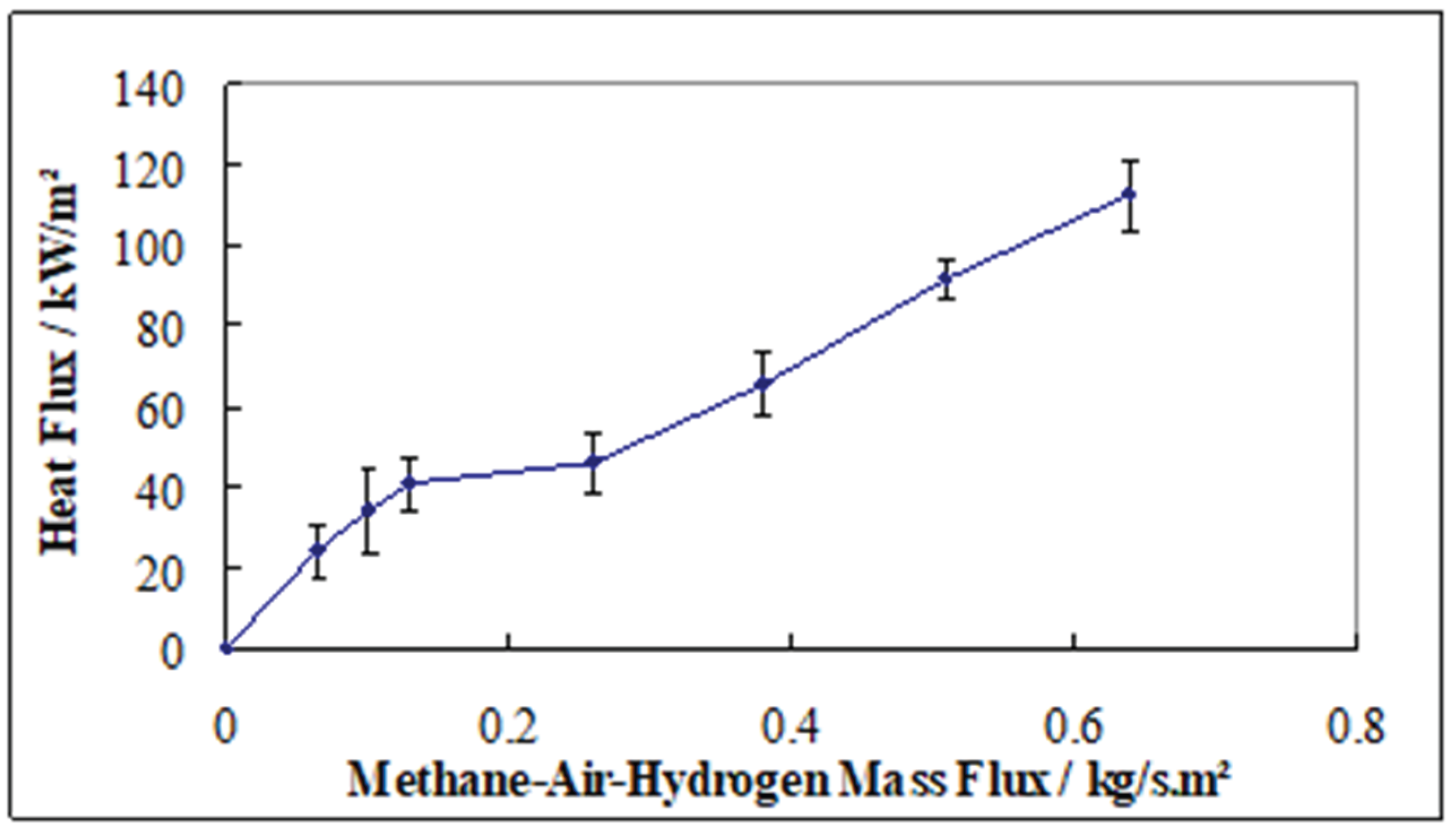
Figure 7.
Heat flux for 20%-hydrogen, 80%-methane-air flame for H=1.5 cm, Ф=1.
As evident from the graphs, the maximum errors occur for very small velocities (0.05-0.08 m/s) in all three cases and are around 22-25%. At higher velocities, the errors reduce to about 7-15%.
5. Conclusions
Using a new technique (both side LEDs), the measurements of surface temperatures and heat fluxes in stagnation flow flames were conducted with precision. For a single stoichiometry ratio and a fixed distance between the stagnation plate and the burner, the study investigated methane–air and hydrogen–methane–air flames at ambient pressure, examining their behavior as a function of mass flux.
The distance was selected to stabilize a flame that was almost one-dimensional and could be accurately modelled using sophisticated chemistry. An alumina plate was coated on both sides with thermographic phosphors, which were employed to measure surface temperatures. Both the water-cooled side and the flame impingement side were used to measure the phosphorescence.
Consequently, it is possible to compute the stagnation point heat flux for one-dimensional methane-air flames. Despite the high accuracy of surface temperature readings, there are considerable inaccuracies in the temperature gradients that are determined and, consequently, in the heat fluxes.
Either the unpredictability of the cooling water flow rate or the uncertainty in the plate’s thermal conductivity could be the cause of the significant mistakes. The cooling water flow rate has a significant impact on the temperature measurement.
For additional research on the basic flame wall interaction, this geometry would be ideal. According to the current findings, flame speed is a significant intrinsic component that affects heat transmission from the flame, at least for laminar flames. Because it produces superior results, excitation with LEDs on both sides is preferable to employing a laser. Compared to lasers, LEDs are far less expensive and simpler to use. Therefore, it would be preferable if studies for higher flame velocities were conducted in the future using LEDs as well. The usage of LED will be a very good method for measuring temperature if we achieve good results for the higher velocities as well.
References
- Allison, S.W.; Gillies, G.T. Remote thermometry with thermographic phosphors: Instrumentation and applications. Rev. Sci. Instruments 1997, 68, 2615–2650. [Google Scholar] [CrossRef]
- Khalid, A.H.; Kontis, K. Thermographic Phosphors for High Temperature Measurements: Principles, Current State of the Art and Recent Applications. Sensors 2008, 8, 5673–5744. [Google Scholar] [CrossRef] [PubMed]
- Brübach, J.; Zetterberg, J.; Omrane, A.; Li, Z.; Aldén, M.; Dreizler, A. Determination of surface normal temperature gradients using thermographic phosphors and filtered Rayleigh scattering. Appl. Phys. B Laser Opt. 2006, 84, 537–541. [Google Scholar] [CrossRef]
- Brübach, J.; Pflitsch, C.; Dreizler, A.; Atakan, B. On surface temperature measurements with thermographic phosphors: A review. Prog. Energy Combust. Sci. 2013, 39, 37–60. [Google Scholar] [CrossRef]
- Childs, P.R.; et al. Review of temperature measurement. Review of scientific instruments 2000, 71, 2959–2978. [Google Scholar] [CrossRef]
- Salem, M.; Staude, S.; Bergmann, U.; Atakan, B. Heat flux measurements in stagnation point methane/air flames with thermographic phosphors. Exp. Fluids 2010, 49, 797–807. [Google Scholar] [CrossRef]
- Elmnefi, M.S.; et al. , Heat flux from stagnation-point hydrogen-methane-air flames: experiment and modelling. Heat Transfer XIII: Simulation and Experiments in Heat and Mass Transfer 2014, 83, 401. [Google Scholar]
- Jenkins, T.P.; Hess, C.F.; Allison, S.W.; I Eldridge, J. Measurements of turbine blade temperature in an operating aero engine using thermographic phosphors. Meas. Sci. Technol. 2020, 31, 044003. [Google Scholar] [CrossRef]
- Feist, J.P.; Heyes, A.L.; Seefelt, S. Thermographic phosphor thermometry for film cooling studies in gas turbine combustors. Proc. Inst. Mech. Eng. Part A: J. Power Energy 2003, 217, 193–200. [Google Scholar] [CrossRef]
- Pflitsch, C.; Siddiqui, R.; Atakan, B. Phosphorescence properties of sol–gel derived ruby measured as functions of temperature and Cr3+ content. Appl. Phys. A 2007, 90, 527–532. [Google Scholar] [CrossRef]
- Pflitsch, C.; Siddiqui, R.A.; Eckert, C.; Atakan, B. Sol–Gel Deposition of Chromium Doped Aluminium Oxide Films (Ruby) for Surface Temperature Sensor Application. Chem. Mater. 2008, 20, 2773–2778. [Google Scholar] [CrossRef]
- Brübach, J.; Janicka, J.; Dreizler, A. An algorithm for the characterisation of multi-exponential decay curves. Opt. Lasers Eng. 2009, 47, 75–79. [Google Scholar] [CrossRef]
- Kee, R.J.; Coltrin, M.E.; Glarborg, P. Chemically reacting flow: theory and practice; John Wiley & Sons, 2005. [Google Scholar]
- Baton, U.N. An introduction to error analysis; John R. Taylor, 1997; pp. 133–134. [Google Scholar]
Figure 1.
Schematic of the experimental setup.
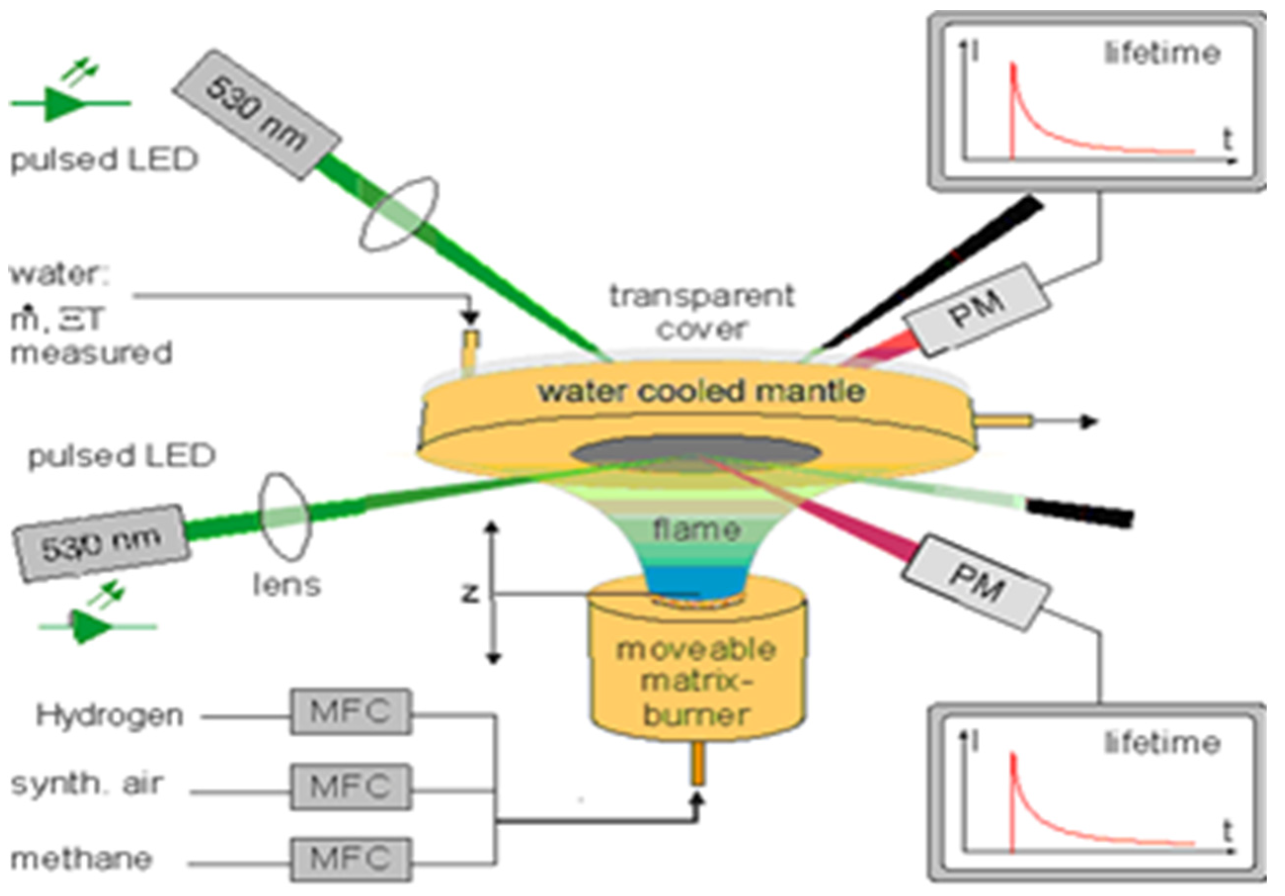
Figure 2.
Surface temperature measurement at (H = 1.5 cm, Ф=1) for various percentages of hydrogen in methane-air flame.
Figure 2.
Surface temperature measurement at (H = 1.5 cm, Ф=1) for various percentages of hydrogen in methane-air flame.
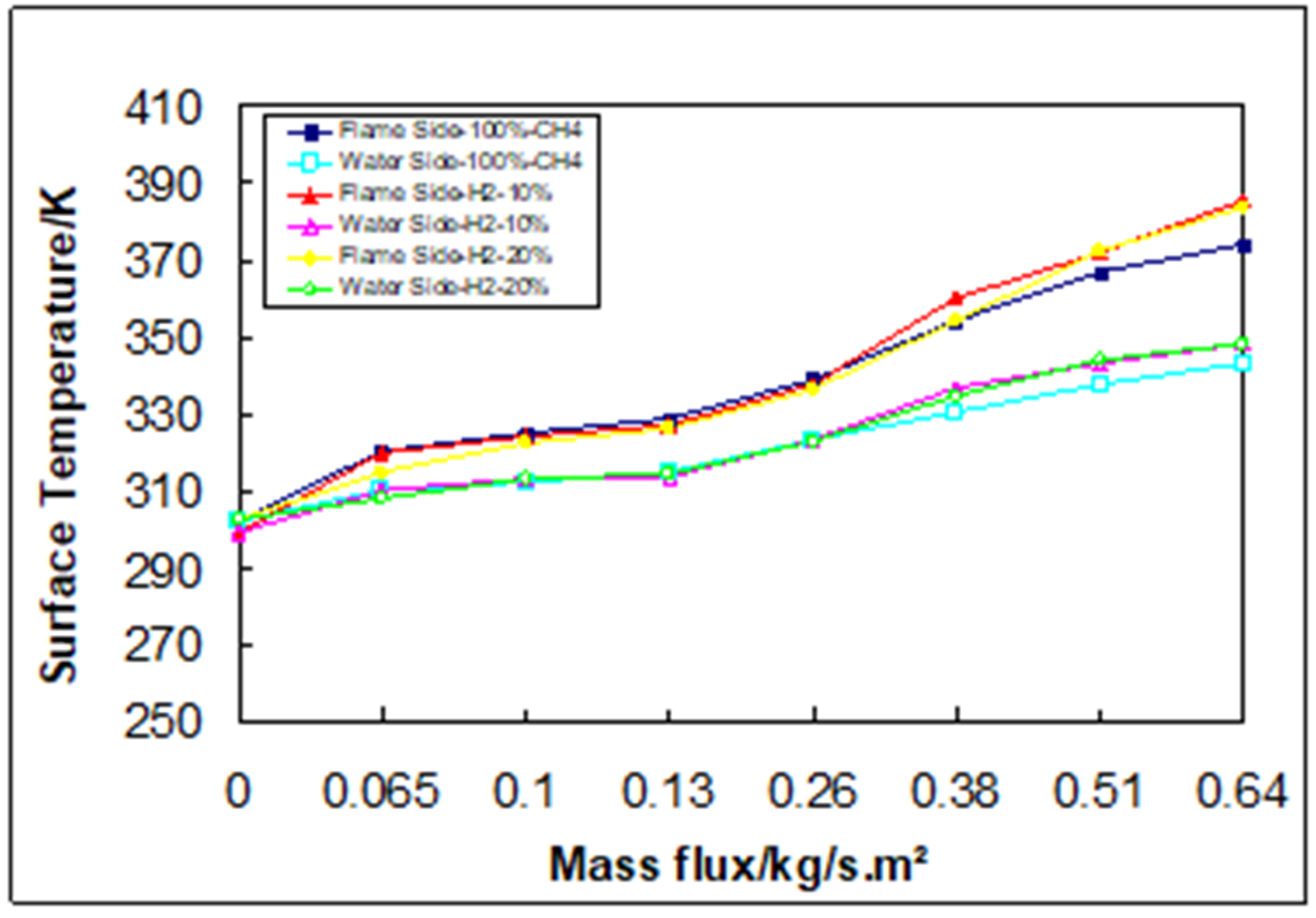
Figure 3.
Stagnation point heat fluxes for stoichiometric flames with 0%, 10% and 20% hydrogen.
Disclaimer/Publisher’s Note: The statements, opinions and data contained in all publications are solely those of the individual author(s) and contributor(s) and not of MDPI and/or the editor(s). MDPI and/or the editor(s) disclaim responsibility for any injury to people or property resulting from any ideas, methods, instructions or products referred to in the content. |
© 2025 by the authors. Licensee MDPI, Basel, Switzerland. This article is an open access article distributed under the terms and conditions of the Creative Commons Attribution (CC BY) license (http://creativecommons.org/licenses/by/4.0/).
Copyright: This open access article is published under a Creative Commons CC BY 4.0 license, which permit the free download, distribution, and reuse, provided that the author and preprint are cited in any reuse.


