Submitted:
23 July 2025
Posted:
25 July 2025
You are already at the latest version
Abstract
The vacuum drying of cellulose-based insulation is an essential step in the transformer production process which usually consists of both heat and vacuum application. The moisture inside the cellulose insulation during this process is transferred by various transport mechanisms, some of which could be affected by temperature of the insulation as well. Furthermore, the conditions inside the vacuum chamber are generally transient and highly dynamic depending on the process control strategy and could include various types of phenomena such as gas expansion during the pump down process or heat transfer by radiation. Mathematically speaking, the above-mentioned conditions will have influence on the drying rate by altering the boundary conditions of heat and mass transport equations. In this study, a mathematical model that considers the process at both the scale of the cellulose insulation and the scale of the vacuum chamber is presented. By introducing a simplified drying system with two-point process control, a model test case and drying case were simulated. Model results demonstrated that chamber dynamics significantly affect drying behaviour. The proposed model could thus facilitate the estimation of total energy consumption and process duration, offering a valuable tool for optimization of vacuum drying procedures.
Keywords:
transformer cellulose-based insulation
; vacuum drying
; dual-scale modelling
; radiation heat transfer
; pump-down
; non-equilibrium moisture content
1. Introduction
It is a well-established fact that the moisture inside the cellulose-based insulation increases the aging rate and shortens the service life of the apparatus [1]. To attain acceptable level of residual moisture content, before being put into service, the transformers are subjected to a thorough drying process which typically involves cyclic heating and vacuum application [2,3].
When it comes to establishing the control strategy for cellulose insulation drying process, the manufacturers frequently rely on experience [3] which is the reason why some recent works have been focused on mathematical modelling of moisture dynamics inside the non-impregnated cellulose insulation. Namely, by having at disposal a reliable and flexible model of vacuum drying process, one can improve it in terms of drying time or energy consumption.
A common approach in describing the moisture transport inside the cellulose insulation is by using Fick’s law in which diffusion coefficient is determined empirically. Notable work in this area was done by Du et al. [4] who determined diffusion coefficient for non-impregnated pressboard. Afterwards, this work was extended by García et al. [5] and Villarroel et al. [6] who experimentally determined the moisture diffusion coefficient in the transformer paper as a function of temperature, moisture content and thickness of the insulation. The similar methods were more recently used by Wang et al. [7] to additionally allow for the effects of insulation ageing on the value of moisture diffusion coefficient.
While results of those models are in good agreement with experimental values, as an intrinsic property of the material, it is not physically based for the diffusion coefficient to be dependent on the dimensions of the sample such as thickness. As stated in [8,9,10] this is a clear indicator that the drying process cannot solely be described by the Fick’s law which was also noticed by García et al. [11] who demonstrated that the thickness dependence of the diffusion factor is not a consequence of interlayer spaces or voids but rather a compensation for inaccuracy of the used diffusion model.
This shortcoming of the classical Fickian description of moisture transport was also recognized by Kang et al. [12] who used a Langmuir model to study the moisture dynamics. This model is based on assumption that the moisture contained within the insulation can be separated into free and bound moisture which are mutually convertible. To extract the bound moisture, it first needs to be transformed into a free moisture which is then transported according to the Fick’s law. Additional parameters of this model are adsorption and desorption coefficients which were determined by fitting the analytical solution of the Langmuir model to the experimentally obtained drying curves. The comparison between the models showed that the Fick model significantly underestimates the necessary drying time of the pressboard.
On the other hand, Brahami et al. [3] adopted an empirical model to describe the drying of the transformer insulation. This model additionally considers degradation of the cellulose insulation due to its exposure to oxygen and elevated temperatures thus providing a mathematical tool for manufacturers to determine the desired compromise between energy consumption and drying time of the process.
All the above-mentioned works adopt assumption of the uniform temperature distribution inside the cellulose insulation. Although heat diffuses through insulation faster than moisture does, there are indications that considerable temperature gradients through cellulose insulation might exist even in later stages of the drying process. They might be caused by local cooling due to the evaporation of water vapor from the cellulose fibres [13] or uneven heating [14]. Furthermore, as drying process consists of series of cycles of heating and vacuum application, transient periods will occur in-between the phases, making it unclear on how boundary conditions on the interface between cellulose insulation and chamber atmosphere should be imposed in those periods. The vacuum chamber atmosphere also interacts with the cellulose insulation through the exchange of heat and mass thus making the whole problem strongly coupled. Accurately capturing this behaviour requires a modelling framework that accounts for both internal dynamics of the cellulose insulation and the surrounding chamber atmosphere. This complexity has been previously addressed in other fields such as wood vacuum drying [15,16,17,18] and pharmaceutical freeze drying [19] where dual-scale modelling approach has been used. The basic idea is to introduce a computational fluid dynamics (CFD) [20] or simplified zero-dimensional (0D) models at the scale of the dryer thus extending the existing (macroscale) model of heat and mass transfer through the porous media. Such models enable more accurate predictions of energy consumption and drying time thus supporting the process analysis and optimization.
In this study, a comprehensive mathematical model that describes the vacuum drying process at both the scale of the cellulose insulation and at the scale of vacuum chamber is presented. The model is implemented in Python and employed to simulate various process configurations. Numerical experiments conducted for a simplified drying system highlight the influence of key model parameters and demonstrate the model’s potential as an effective tool for analysing and optimizing the vacuum drying process of transformer cellulose-based insulation.
2. Mathematical Model
The mathematical model that describes the vacuum drying process of transformer cellulose-based insulation is structured to capture the relevant physical phenomena occurring within the drying system. The following subsections first provide a description of the observed drying system, followed by the formulation of the governing equations, interface conditions between the cellulose and the chamber atmosphere, initial conditions and numerical solution procedure.
2.1. Drying System Description
In this study, a simplified yet sufficiently sophisticated drying system is considered, designed to enable control of the two primary process variables: drying temperature and pressure. As illustrated in Figure 1, the system consists of a thermally insulated vacuum chamber with two ports. The first port is connected to a vacuum pump through the suction line, with a throttle valve installed to reduce or completely shut off the pumping speed when necessary. Additionally, to ensure that no significant over-pressure occurs and to enable the venting process at the end of each vacuum phase, a vacuum chamber is equipped with a valve that has both breathing and venting function. Lastly, the heating of the cellulose insulation is achieved with infra-red (IR) heaters mounted on the inner walls of the vacuum chamber shell. In addition to radiation, the heat is also being transferred by natural convection since no fan or forced air circulation is employed.
Inside the chamber, transformer samples with simple geometry are placed. Each sample consists of cellulose insulation paper wrapped around a cylindrical metal core, serving as a reasonable approximation for actual transformer. In that case, one can assume that the outer side of the sample is completely exposed to the vacuum chamber conditions and inner side is thermally insulated and impermeable to mass transfer. The number, size and spatial arrangement of the samples can vary depending on the available space inside the vacuum chamber.
2.2. Governing Equations at the Scale of the Cellulose Insulation
Unlike previous studies, different approach is considered in modelling the heat and mass transport through the cellulose insulation. Knowing that the transformer insulation is composed of the cellulose fibres containing moisture and pores filled with humid air (Figure 2), it is assumed that the moisture inside the fibres is practically immobile and that its transport is achieved in the form of water vapor through the pore space by means of diffusion and convection. Furthermore, a local non-equilibrium is assumed between cellulose fibres and humid air inside the pores. The moisture content of the fibres will tend to reach the equilibrium state which will then result in local moisture transport between the fibres and humid air inside the pores. That is, moisture inside cellulose fibres will either be absorbed or desorbed, depending on the difference between current moisture content and equilibrium moisture content.
The cellulose insulation usually has cylindrical shape with radial dimensions much smaller than height. Additionally, the conditions on the outer and inner boundaries are assumed to be uniform along the perimeter and height therefore making it reasonable to assume that variations of physical fields in axial and azimuthal directions can be neglected. In that case, the transport of heat and mass is considered only in the radial direction, as shown on Figure 1.
The pore space of the insulation can be filled with dry air and water vapor so those species must be conserved. The conservation law for dry air has the form of convection-diffusion equation:
whereas, in conservation law for water vapor additional source term emerges due to the absorption or desorption of moisture from the cellulose fibres:
In equations (1) and (2), (kmol/m3) and (kmol/m3) are molar densities of air and water vapor respectively. Both water vapor and dry air are assumed to behave like ideal gases, so following relations hold:
where is the total pressure of the gaseous phase with and being partial pressures of water vapor and dry air, respectively.
The equivalent binary diffusivity in equations (1) and (2) includes Knudsen effect that could arise during vacuum phases and is given by the following relation [18]:
where, is an effective binary diffusivity of water vapor and dry air mixture, expressed as a function of absolute temperature and pressure [21]:
and (m2/s) is a Knudsen diffusivity that should be empirically determined during the model calibration [18].
The velocity of the gaseous phase is calculated according to Darcy’s law:
where, (m2) is an effective permeability coefficient of the cellulose insulation obtained with Klinkenberg correction to account for the slip effects at low pressures [22]:
In the equation (9) (m2) is an absolute permeability that is measured at large pressures and (Pa) is a Klinkenberg correction factor that increases with decrease of absolute permeability .
Moisture inside the cellulose fibres can be absorbed or desorbed depending on the equilibrium moisture content which it tends to reach. The mass conservation law for moisture contained in the cellulose fibres has the following form:
where (1/s) is an internal overall mass transfer coefficient whose value depends on the resistance of the moisture transport from the inner parts of the cellulose fibres to the pore-fibre interface. It also strongly depends on the total pore-fibre interface surface area per unit of volume of the insulation. It is not an easy task to accurately calculate so a simplified approach is undertaken in this work by assuming that it has a constant value that should be empirically determined.
Dry-basis equilibrium moisture content in equation (10) is a function of temperature and water activity of the surrounding media. An analytical form with temperature and water vapor partial pressure as independent variables was early given by Fessler et al. [24] and later corrected by Du et al. [25]. This expression, although accurate for low moisture contents, might give non-physical results for water activities closer to unity. Przybylek et al. [23] calculated the parameters of the GAB (Guggenheim, Anderson and de Boer) sorption isotherm model based on the experimental results for Kraft paper samples with different ageing degrees. This model gives accurate results in a wider range of relative humidities (Figure 3) and was used in calculating equilibrium moisture content in this model.
Since water activity was not chosen as a dependent variable of the model, it is expressed in terms of molar density and temperature. This follows from the definition of water activity and the assumption that dry air and water vapor are ideal gases.
In the above equation, is water vapor saturation pressure that can easily be calculated for a known temperature [26].
Equilibrium moisture content according to the GAB model is calculated from the following expressions:
For more detailed explanation of GAB model and physical meaning behind parameters , , , and , one can refer to the work of Staudt et al. [27]. The values of the above parameters used for this model are taken from [23] and are given in Table A1 in the Appendix.
To close the system of the governing equations at the scale of the cellulose insulation, conservation of energy needs to be applied. Unlike moisture concentration, an assumption of local thermal equilibrium between cellulose fibres and gaseous phase inside the pores is assumed. The specific heat of the insulation is assumed to be equal to the specific heat of the solid cellulose fibres, so the conservation of energy reads:
where (W/(m∙K)) is an effective thermal conductivity of the cellulose insulation and (J/kg) is specific heat of water evaporation.
2.3. Governing Equations at the Scale of the Vacuum Chamber
The governing equations at the scale of the vacuum chamber are derived under the assumption that temperature, pressure and molar densities of water vapor and dry air are uniformly distributed fields within the available volume (m3) inside the vacuum chamber. Moreover, the temperature fields of the chamber walls and IR heaters are also considered uniform and dependent only on time variable.
The gaseous phase (water vapor and dry air) can enter the chamber through the venting valve and leave the chamber through the pressure relief valve or during the pump down process. At the interface between the transformer cellulose insulation and vacuum chamber atmosphere, the molar flow rate of gaseous phase can be directed either inward or outward. The conservation laws are thus expressed accordingly:
After expanding and rearranging the terms, the following equations are obtained:
In the above equations and are volume flow rates through venting valve and pressure relief valve, respectively. Since a single valve is used for both venting and pressure relief, volume flow rates and are mutually excluding (only one at the time can have non-zero value). In view of that, and are calculated as follows:
where (Pa) and (Pa) are ambient and chamber pressures respectively. During the venting process, a choked flow might occur, however, since venting is relatively rapid part of the process in comparison to other phases, the chocked flow phenomena is not considered in this work.
The pumping speed at the outlet port of the vacuum chamber (effective pumping speed), (m3/s), is generally different from the pumping speed at the inlet of the vacuum pump. The inlet pumping speed can be found in the manufacturer’s datasheet as a function of the pressure at the vacuum pump inlet . To calculate effective pumping speed, throughput continuity equation under the assumption of isothermal flow in the suction line is used:
To obtain the pressure at the inlet of the vacuum pump, effective pumping speed from the equation (21) is substituted into the equation for the conductance of the suction line:
For a given conductance (m3/s) and pressure inside the vacuum chamber , equation (22) is solved for pressure at the inlet . This pressure is then substituted into equation (21) to obtain effective pumping speed which is then used in the governing equations. More details regarding the calculation of the effective pumping speed can be found in [28].
The energy conservation laws for dry air and water vapor can be incorporated into a single equation since both species are at the same temperature . Accumulation of the internal energy of the open system is due to the convective heat flow rate and enthalpy flows through the boundary:
The enthalpy difference can be written as:
where is cellulose insulation surface temperature of the i-th transformer.
Atmosphere in the chamber can convectively exchange heat with chamber walls, IR heaters and cellulose insulation of the transformers. The term in equation (23) can therefore be written as:
where , and are convective heat transfer coefficients at the interface between chamber atmosphere and other components: transformer cellulose insulation, IR heaters and chamber walls.
After combining equations (23), (24), (25) and rearranging, the final form of the energy equation is obtained:
where (kmol/m3) is molar density of ambient air and is specific heat ratio of the gaseous phase inside the vacuum chamber.
Energy equation for the IR heaters, derived in a similar fashion, reads:
where (W) and (W) are radiative heat flow rate from heaters surface and input electrical power respectively.
Vacuum chamber walls energy equation reads:
where is radiative heat flow rate at wall surface, is thermal conductivity of the vacuum chamber thermal insulation and is thermal insulation thickness.
2.3.1. Convective Heat Transfer Coefficients Calculation
It would be wrong to assume that convective heat transfer coefficients don’t change during the vacuum drying process. Rarified atmosphere at low pressures causes convective heat transfer to diminish. To calculate the heat transfer coefficients at low pressures, a model from Gonzales et al. [29] which gives relation between Nusselt and Rayleigh number for natural convection along a vertical plate is used:
where and are dimensionless quantities defined as:
where is a height of the j-th surface. Every surface is considered to behave like vertical plate, even the transformers (vertical cylinders) since their height is much larger than outer diameter. The properties with j in index are evaluated for the temperature of the j-th surface.
Equation (29) is valid for Rayleigh numbers in the range from 10-2 to 105, a condition that is satisfied throughout this type of the drying process.
2.3.2. Radiative Heat Flow Rates Calculation
Under the assumption that all surfaces in the system are grey and diffuse, balance of the radiative het flow rates can be written [30]:
where is the number of surfaces that exchange heat by radiation, is total emissivity of the j-th surface, is the view factor from surface k to surface j, is the surface area of the j-th surface and is Kronecker delta operator that is equal to unity when indices k and j are the same and zero otherwise.
Equation (32) written down for all the surfaces results in linear system of equations which is then solved for radiative heat flow vector .
2.4. The Interface Between Transformer Cellulose Insulation and Vacuum Chamber Atmosphere
To close the system of the governing equations, the interface between transformer cellulose insulation and chamber atmosphere should be properly modelled.
It is assumed that the partial pressures of water vapor and dry air at the interface are the same as in the chamber atmosphere. Therefore, for all transformers, the following equations hold:
however, since every transformer can have different temperature field, the following Dirichlet boundary conditions are used for i-th transformer:
From equations (33) and (34) it consequently follows that the total pressure at the interface is equal to the pressure in the vacuum chamber:
On the inner radius, zero molar flux boundary conditions are imposed:
The boundary condition for energy equation (14) is a Robin-type and includes both convective and radiative heat fluxes:
where is radiative heat flow rate at the i-th transformer surface which can either be transfer from the surface (negative) or onto the surface (positive).
On the inner radius, zero heat flux is imposed:
For known fields of molar densities and temperature, molar fluxes of water vapor and air at the interface between the transformer cellulose insulation and vacuum chamber atmosphere can be calculated:
These fluxes are then substituted into the governing equations (17), (18) and (26).
2.5 Initial Conditions
All the components of the vacuum drying system as well as cellulose insulation are assumed to be at ambient temperature. The gaseous phase inside the pores of the cellulose insulation and atmosphere of the vacuum chamber are under ambient pressure and ambient relative humidity. In that case, the initial moisture content of the cellulose insulation is equilibrium moisture content for ambient air. The initial conditions are as follows:
2.5 Numerical Solution Procedure
The governing equations (1), (2), (10) and (14) at the scale of cellulose insulation and governing equations (17), (18), (26), (27) and (28) at the scale of vacuum chamber, along with all the boundary conditions and constitutive relations form a nonlinear coupled PDE-ODE system.
One way to decouple the system and find the solution would be to solve the ODE system with guessed values of cellulose insulation fields. The ODE solutions can then be used to define necessary boundary conditions for which PDE system is solved and the better guess for cellulose insulation fields is obtained. This is the iterative procedure that is repeated until convergence is achieved. In this study, however, solving a coupled PDE-ODE system was addressed using an alternative approach.
Firstly, all the equations were scaled so that variables of the model have order of magnitude around unity or less. Then spatial derivatives in governing equations ((1), (2), (14)) and in interface equations ((38), (39), (40), (41), (42), (43)) were discretized using second order finite difference scheme. This leads to a large system of ODEs which is then solved using the LSODA method implemented in in the SciPy package for Python programming language [31]. This method automatically switches between Adams (non-stiff part of solution) and implicit BDF (stiff part of the solution) methods. Relative and absolute tolerances were set to 10-5 and 10-7 respectively. A similar methodology for solving PDE-ODE systems was investigated by Filipov et al. [32] so readers interested in further details are referred to their work.
3. Results and Discussion
Numerical simulations for all the cases studied below were run with the parameter values and relations listed in the Table A1, Table A2, Table A3 and Table A4 given in the Appendix section. The exceptions are two parameters: absolute permeability and internal overall mass transfer coefficient for which series of values were used to study their influence on the moisture dynamics.
The vacuum dryer dimensions correspond to those of a laboratory-scale vacuum chamber that is used at our institution. Likewise, the choice of vacuum pump and its characteristic pumping speed correspond to a commercially available unit (VD 65, Leybold) currently in use.
Apart from the parameter values and relations, to solve the system of governing equations, the values of the view factors need to be calculated beforehand. This was done firstly by generating rudimentary geometry of the surfaces that exchange heat by radiation, namely, the IR heaters, transformer samples and vacuum chamber walls, as shown on Figure 4. The generated mesh is a pre-requisite for computation of view factors; however, it is not necessary to calculate them for all cells since reciprocity and summation rules can be applied [30].
Furthermore, due to the spatial layout of the transformer samples, three representative ones, corner, side and center transformer sample, as pointed out on the Figure 4 can be identified out of the total of nine. Since these samples are exposed to a distinct radiative conditions, it is sufficient to compute view factors for only these three and thus significantly save computational resources.
The calculation of view factors was done with pyviewfactor [34], a Python package that utilizes PyVista [33] functionalities, such as ray tracing that was used for checking the shadowing of the cells. The calculated view factors subsequently used in equation (32) are listed in Table 1.
The drying process described by this model can be controlled by on/off switching of three main components:
- IR heaters (when off, W)
- Vacuum pump (when off, m3/s)
- Venting/pressure relief valve (when off, )
Depending on the component type and timing of the switching, the process can discretely by controlled in numerous ways. In this work, test case and drying case were studied.
3.1. Test Case Results
Firstly, to analyze the results in terms of spatio-temporal physical fields, a short-duration test case was simulated. The main component states and their corresponding durations are listed in Table 2 and as such provide enough information to define the test case process. The states of the components are defined in such way that all the commonly encountered conditions, such as IR heating, vacuum pump-down and venting are encompassed in this numerical simulation. The test case therefore consists of 2.5-hour IR heating period with the pressure relief valve open to the atmosphere, followed by 2.5 hours of vacuum pump-down with heaters turned off, ending with a 2.5-hour venting period during which the heaters remain off.
As heaters are activated, the temperature of cellulose insulation increases. This reduces the equilibrium moisture content of the cellulose fibers according to equation (12). Since cellulose fibers tend to reach a lower moisture content state, desorption of moisture occurs consequently making the pores of the cellulose insulation more saturated with water vapor, as seen on Figure 5a. The developed gradient of the water vapor molar fraction acts as a driving force for equimolar diffusion of dry air and water vapor within the pores. The diffusive flux during the heat-up period, however, is not unidirectional; it changes direction at certain radius which is the consequence of water vapor molar ratio maxima at that point. This is not surprising; since heat is transferred to the outer surface only, the molar density of water vapor is highest near the surface and lower at the very interface. A similar thing happens with the pressure field, as seen on Figure 6b. On the same plots, an under-pressure region can also be identified near the internal surface. This is a consequence of the combined effect of dry air diffusing outwards and absorption of water vapor that diffuses inwards, toward the parts that are still unheated.
The temporal variations of physical fields for corner and side transformer samples are nearly identical, which is expected given the relatively similar values of the view factors from IR heaters to these samples. In contrast, the center transformer sample is completely obstructed by the surrounding samples, so the radiative flux reaching its surface originates from neighboring samples and not directly from the heaters. This manifests as a slower increase in temperature (Figure 5c) and slower decrease of moisture content (Figure 5d). Moreover, the moisture content of the center transformer even shows a slight increase during the heating period near the outer surface which has to do with the variation of molar density in the vacuum chamber atmosphere.
Water vapor is convectively and diffusively transferred at the surface of corner and side transformer samples to the vacuum chamber atmosphere according to the interface equation (42). Furthermore, both dry air and water vapor exit the chamber through the venting/over pressure valve due to the rising pressure. This results in an increase in water vapor and a decrease in dry air molar density as shown in Figure 7a. The elevated water vapor molar fraction and lower surface temperature of the center transformer sample correspond to higher equilibrium moisture content causing a slight absorption of water vapor at the surface of the center transformer sample.
When the vacuum pump down period starts, dry air molar density within the pores rapidly drops (Figure 5b) and the similar decrease is observed in the vacuum chamber (Figure 7a). In contrast, water vapor molar density remains nonzero due to continued desorption from the cellulose fibers (Figure 5a). As a result, pressure gradient develops along thickness of the cellulose insulation (Figure 6b) which gives rise to a more intensive convective transport and consequently to an increase in the drying rate. The diffusive flux in this period is zero since water vapor molar fraction is uniform and equal to unity (Figure 6a).
During the vacuum chamber venting period, dry air diffuses into the cellulose insulation leading to an increase in its molar density. The elevated dry air concentration combined with a still relatively high temperature causes desorption of moisture in the inner layers and in consequence an increase in pressure shortly after opening the venting valve.
Figure 7b shows temporal variations of surface temperatures inside the vacuum chamber. Among the transformer sample surfaces, the side transformer sample surface exhibits the most rapid increase in temperature that is attributed to the highest view factor from the heaters (Table 1). A similar trend is observed for the corner sample surface, though its temperature is slightly lower due to a lower value of view factor. On the other hand, a center transformer sample surface shows significantly slower increase in temperature and additionally maintains lower temperatures throughout the entire heating period. This behavior is clearly a result of the surrounding samples obstructing the center one from direct exposure to the heaters.
These results suggest that the surface temperature of the sample most exposed to the IR heaters (in this case, side transformer sample) is a suitable candidate for use as a control variable in terms of temperature control. The choice of highest temperature is due to the upper temperature limit imposed to prevent rapid degradation of the cellulose insulation.
The temperature of the chamber atmosphere initially increases mostly due to convective heat transfer from the surfaces within the chamber. A sudden drop is observed when the pump down period starts, which can be attributed to the expansion of the gaseous phase. The opposite effect occurs when the venting valve opens. As ambient air rushes inside the chamber it compresses the gaseous phase, resulting in sharp increase in temperature. Lastly, vacuum chamber walls exhibit the slowest temperature increase due to their relatively high heat capacity.
3.2. Impact of the and Parameters
The parameters whose impact is investigated are absolute permeability and internal overall mass transfer coefficient . All other parameters are either held constant or can be calculated from the relations, both of which are provided in the Table A1 in the Appendix. Moreover, the states of the main components for all simulations are the same as in the test case (Table 2). Lastly, given the small difference in physical fields between the corner and side transformer samples, only the center and side samples are observed in this analysis.
To evaluate the influence of the above-mentioned parameters, an average moisture content of the cellulose insulation was computed using the following equation:
Figure 8a illustrates the influence of the internal overall mass transfer coefficient on the evolution of average moisture content during the test case process. As increases, the characteristic time for equilibration decreases, causing local absorption and desorption processes to become significantly faster than diffusive and convective transport. In that case, local equilibrium can be assumed to occur instantaneously, allowing the moisture content field to be computed directly using equation (12) for given fields of water vapor molar density and temperature. In contrast, lower values of lead to more inert moisture dynamics characterized by reduced drying rates.
The influence of absolute permeability is illustrated in Figure 8b. As shown, higher permeability results in an increased drying rate during the vacuum period, which is a direct consequence of enhanced convective transport, consistent with Darcy’s law (equation (8)). Conversely, lower value of result in lower drying rate in vacuum period. It is also observed that value of has a negligible effect on the drying rate during the heating period, at least while pressure gradients remain low. However, as pressure gradients develop, the convective transport becomes more prominent, thereby increasing the sensitivity of the results to the value.
Both and parameters significantly affect the drying rate, yet their values are not easily determined through theoretical means as both are highly dependent on the microstructure of the insulation. The most time-efficient approach would therefore be to estimate these parameters through model calibration, by comparing the simulation results with experimental data.
The Knudsen diffusivity parameter was also examined as a part of this analysis and it was found to have no significant influence on the drying rate. This observation is consistent with the model formulation. Specifically, equation (6) which indicates that the contribution of becomes relevant at low pressures. However, under vacuum conditions, the molar fraction of water vapor approaches unity and becomes uniform across the domain, eliminating concentration gradients and, consequently, diffusive transport.
3.3. Drying Case Results
The drying case was defined to resemble a process with conditions typically met in transformer manufacturing procedure, consisting of a sequence of alternating heating and vacuum phases [35,36]. To maintain the specified temperature and pressure levels throughout the process, a temperature and pressure two-point (on/off) control was implemented in the simulation. The operational states of the main components and their respective durations are summarized in Table 3.
To ensure that the cellulose insulation does not exceed the upper temperature limit of 130 °C, the controlled temperature was chosen to be the surface temperature of the side transformer sample, as explained in the previous section. Figure 8 presents the temporal variations of the surface temperatures and the innermost layer temperatures of the corresponding transformer samples. The same figure also displays the variation in pressure of the chamber atmosphere over time. Significant temperature gradients across the thickness of the cellulose insulation are evident. Their negative signature is characteristic of one-sided heating and is unfavorable in terms of drying rate [10].
Furthermore, the obstructed center sample remains at somewhat lower temperature throughout the entire drying process, a condition that is expected to extend the overall drying time. The observed decrease in temperature of the transformer samples during the vacuum phases results from radiative cooling due to the turned off IR heaters as well as cooling due to the water vapor evaporation. This is evident from Figure 9, where each successive vacuum phase is characterized by a smaller drop in surface temperatures, indicating a decline in evaporative cooling as the drying rate diminishes over time.
Convective and radiative heat fluxes at the surface of side and center transformer samples are illustrated in Figure 10. The results demonstrate that convective heat flux diminishes during the vacuum phases which is consistent with the reduction of the convective heat transfer coefficient at low Rayleigh numbers, as described by equation (29). For all transformer samples, convective heat flux remains generally negative due to the lower temperature of the vacuum chamber atmosphere relative to the sample surfaces. Peaks in convective heat flux appearing at the onset of each vacuum phase result from the rapid cooling of the vacuum chamber atmosphere caused by its expansion during pump-down. On the other hand, radiative heat flux is characterized by periodic oscillations which arise from the on/off temperature control achieved by changing the operating states of the heaters and thus the emitted radiative flux.
Figure 11a illustrates the molar flux at the surface of side and center transformer throughout the drying process. Initially, a diffusion dominates, with diffusive flux reaching a peak before gradually decreasing. This behavior results from the rising water vapor molar fraction in the chamber, which eventually causes the diffusive flux to vanish entirely. Not long after the start of the process, as insulation continues to heat up and water vapor gets desorbed from the cellulose fibers into the pore space, pressure gradients begin to develop across the insulation thickness, giving rise to convective molar transport. The convective flux reaches its peak after the diffusive flux and then declines as the pressure field gets more uniform.
To extract the water vapor from the pore space of the insulation, at some point, chamber pressure must be reduced to regain an increase in convective molar flux. As these gradients again start to diminish, the chamber is vented and temperature control is reactivated. At the beginning of the next heating phase, the molar fraction of the water vapor is no longer uniformly distributed since ambient air is introduced which then results in subsequent increase in diffusive flux.
Periods of increased molar flux correspond to a higher drying rate intervals as shown in the drying rate time evolution plot for side and center transformer sample in Figure 11b. For both transformer samples, each successive phase exhibits a lower drying rate values. Interestingly, though, the center transformer sample showing a lower drying rate at the beginning of the process eventually surpasses the side sample. This behavior can be attributed to its higher moisture content throughout the process which makes it more responsive to subsequent heating and vacuum phases.
The drying curves of all three transformer samples are shown on Figure 11c. The side and corner samples, both exposed to similar radiative conditions, exhibit nearly identical drying behavior. In contrast, the center transformer sample initially experiences a slight increase in moisture content. This is attributed to a rapid increase in water vapor molar fraction of the vacuum chamber atmosphere (primarily due to moisture desorption from the surrounding samples) and comparatively slow heating of the center sample. As the center sample heats up, its drying rate changes the signature, however, its moisture content remains elevated throughout the entire process. This observation clearly suggests that the overall drying duration is dictated by the moisture dynamics of the radiatively obstructed regions and cold spots within the cellulose insulation. These challenges are among the reasons why alternative drying technologies, such as low-frequency heating and vapor phase drying [35], are often employed in industrial practice.
The drying case results presented should be interpreted qualitatively, as the underlying model has not been calibrated with respect to key parameter values. Nevertheless, the simulation results suggest that by modifying the controlled values, as well as the timing and duration of heating and vacuum phases, it is possible to influence the drying rate trend and, consequently, the total drying time. As the model accounts for the process at the vacuum chamber scale, it also enables estimation of the total energy consumption of the IR heaters. This allows for process optimization with respect to drying time, energy consumption or a trade-off between the two.
4. Conclusions
This study has presented a detailed mathematical model of the vacuum drying process for transformer cellulose-based insulation accounting for coupled heat and mass transfer phenomena at both the cellulose insulation scale and the vacuum chamber scale. Although the simulations were carried out for a laboratory-scale dryer with a simplified geometry, implementing real dimensions and geometry is largely a matter of parameter adjustment. The presented model could also be adapted to alternative heating methods, such as hot air circulation, by modifying the constitutive relations used to compute the convective heat transfer coefficient or drying with internal heating, by modifying the boundary conditions at the cellulose insulation interface.
By incorporating radiative heat transfer along with view factor computation, the model results have highlighted the influence of the spatial layout of transformer samples, an important practical consideration when setting up the drying process.
Unlike previous studies discussed in the introduction section, the results of this model demonstrate the important role of combining heating and vacuum phases in the drying procedure. While this strategy is already common in transformer manufacturing industry, the present study provides clear physical explanation for its effectiveness.
The model, with its dual-scale formulation, offers a valuable framework for optimizing the drying process with respect to both drying time and energy consumption. However, a major limitation of this model lies in the uncertainty of several cellulose insulation properties that have substantial effect on moisture dynamics. Such are absolute permeability and internal overall mass transfer coefficient as well as sorption isotherm data. These limitations can be addressed through experimental calibration of the model; an essential step planned for our future work.
Author Contributions
Conceptualization, N.B., S.M and N.F.; methodology, N.B.; software, N.B..; writing—original draft preparation, N.B..; writing—review and editing, N.B., S.M. and N.F..; visualization, N.B.; supervision, S.M. and N.F. All authors have read and agreed to the published version of the manuscript.
Funding
This research received no external funding.
Conflicts of Interest
The authors declare no conflicts of interest.
Abbreviations
The following abbreviations are used in this manuscript:
| GAB | Guggenheim, Anderson and de Boer |
| IR | Infra-red |
| PDE | Partial differential equations |
| ODE | Ordinary differential equations |
| 0D | Zero-dimensional |
| CFD | Computational fluid dynamics |
Nomenclature
| Latin symbols | |
| IR heaters surface area, m2 | |
| Transformer cellulose insulation outer surface area, m2 | |
| water activity, - | |
| vacuum chamber walls surface area, m2 | |
| Klinkenberg parameter, Pa | |
| dry air molar density of the vacuum chamber atmosphere, kmol/m3 | |
| molar density of the vacuum chamber atmosphere, kmol/m3 | |
| water vapor molar density of the vacuum chamber atmosphere, kmol/m3 | |
| dry air molar density, kmol/m3 | |
| gaseous phase molar density, kmol/m3 | |
| water vapor molar density, kmol/m3 | |
| effective binary diffusivity (water vapor and dry air), m2/s | |
| equivalent binary diffusivity (water vapor and dry air), m2/s | |
| Knudsen diffusivity parameter, m2/s | |
| i-th transformer convective heat transfer coefficient, W/(m2∙K) | |
| vacuum chamber walls convective heat transfer coefficient, W/(m2∙K) | |
| IR heaters convective heat transfer coefficient, W/(m2∙K) | |
| i-th transformer outer surface molar flux of dry air, kmol/(m2∙s) | |
| i-th transformer outer surface molar flux of water vapor, kmol/(m2∙s) | |
| internal mass transfer parameter, 1/s | |
| absolute permeability of the cellulose insulation, m2 | |
| effective permeability of the cellulose insulation, m2 | |
| Venting/pressure relief valve flow coefficient, m3/s | |
| pressure of the gaseous phase, Pa | |
| dry air partial pressure in the vacuum chamber atmosphere, Pa | |
| water vapor partial pressure in the vacuum chamber atmosphere, Pa | |
| pressure of the vacuum chamber atmosphere, Pa | |
| pressure at the inlet of the vacuum pump, Pa | |
| convective heat flow rate to vacuum chamber atmosphere, W | |
| radiative heat flow rate from IR heaters surface, W | |
| radiative heat flow rate from the surface of the i-th transformer, W | |
| IR heaters input electrical power, W | |
| radiative heat flow from the surface of vacuum chamber walls, W | |
| vacuum pump inlet pumping speed, m3/s | |
| vacuum pump effective pumping speed, m3/s | |
| volume flow rate through pressure relief valve, m3/s | |
| volume flow rate through venting valve, m3/s | |
| radius of the cellulose insulation, m | |
| universal gas constant, 8314.4 J/(kmol∙K) | |
| time variable, s | |
| cellulose insulation temperature, K | |
| i-th transformer cellulose insulation outer surface temperature, K | |
| ambient temperature, K | |
| vacuum chamber atmosphere temperature, K | |
| IR heaters temperature, K | |
| vacuum chamber walls temperature, K | |
| vacuum chamber atmosphere volume, m3 | |
| Darcy’s velocity of gaseous phase, m/s | |
| dry-basis moisture content of the cellulose fibres, kg/kg | |
| dry-basis average moisture content of the cellulose fibres, kg/kg | |
| dry-basis equilibrium moisture content of the cellulose fibres, kg/kg | |
| Greek symbols | |
| dry air specific heat ratio, - | |
| gaseous phase specific heat ratio, - | |
| water vapor specific heat ratio, - | |
| vacuum chamber thermal insulation thickness, m | |
| fibre volume fraction, - | |
| porosity of the cellulose insulation, - | |
| cellulose insulation effective thermal conductivity, W/(m∙K) | |
| cellulose fibre thermal conductivity, W/(m∙K) | |
| vacuum chamber thermal insulation thermal conductivity, W/(m∙K) | |
| cellulose insulation bulk density, kg/m3 | |
| cellulose fibres density, kg/m3 | |
| cellulose fibre tortuosity, - | |
| pore space tortuosity, - | |
| Stefan-Boltzmann constant, 5.67∙10-8 W/(m2∙K4) | |
| gaseous phase dynamic viscosity, Pa∙s |
Appendix

Table A1.
Physical properties of cellulose insulation.
| Parameter | Value/relation | Unit |
|---|---|---|
| Fibre density, | 1550 [37] | kg/m3 |
| Bulk density, | 1000 | kg/m3 |
| Fibre specific heat capacity, | 1340 [37] | J/(kg∙K) |
| Fibre thermal conductivity, | 0.335 [37] | W/(m∙K) |
| Porosity, | - | |
| Fibre volume fraction, | - | |
| Pore tortuosity, | [38] | - |
| Fibre tortuosity, | [38] | - |
| Klinkenberg parameter, | [39] | Pa |
| Knudsen diffusivity parameter, | 10-5 | m2/s |
| Emissivity, | 0.9 | - |
| GAB isotherm parameter, | 0.05128 [23] | kg/kg |
| GAB isotherm parameter, | 0.716 [23] | - |
| GAB isotherm parameter, | 6.1446 [23] | - |
| GAB isotherm parameter, | 323.15 [23] | K |
| GAB isotherm parameter, | 19319.76 [23] | kJ/kmol |
Table A2.
Physical properties of other components
| Parameter | Value/relation | Unit |
|---|---|---|
| Vacuum chamber walls specific heat capacity, | 461 (stainless steel) | J/(kg∙K) |
| Vacuum chamber walls emissivity, | 0.1 | - |
| Vacuum chamber walls thermal insulation conductivity, | W/(m∙K) | |
| IR heaters specific heat capacity, | 800 (ceramics) | J/(kg∙K) |
| IR heaters emissivity, | 0.95 | - |
Table A3.
Process parameters, dimensions and masses of the components
| Parameter | Value/relation | Unit |
|---|---|---|
| Transformer inner radius, | 40 | mm |
| Transformer cellulose insulation thickness, | 50 | mm |
| Transformer outer radius, | mm | |
| Transformer height, | 0.8 | m |
| Transformer surface area, | m2 | |
| Number of transformers in the vacuum chamber, | 9 | - |
| Spacing between transformers | 0.08 | m |
| Vacuum chamber walls mass, | 370.389 | kg |
| Vacuum chamber atmosphere volume, | 1.7567 | m2 |
| Vacuum chamber walls surface area, | 7.86388 | m2 |
| Vacuum chamber shell height, | 1.21 | m |
| Vacuum chamber thermal insulation thickness, | 32 | mm |
| IR heater width, | 62.5 | mm |
| IR heater height, | 0.75 | m |
| IR heaters number, | 4 | - |
| IR heaters total mass, | 2.7 | kg |
| IR heaters total electrical power, | 3000 | W |
| Vacuum pump nominal pumping speed | 65 (Leybold VD65) | m3/h |
| Vacuum pump inlet pumping speed, | linearly interpolated from the data for Leybold VD65 (gas ballast valve closed) | m3/s |
| Suction line conductance, | 0.01 | m3/s |
| Venting/pressure relief valve flow coefficient, | 0.00005 | - |
Table A4.
Dry air and water vapor properties, thermodynamical relations and constants
| Parameter | Value/relation | Unit |
|---|---|---|
| Dry air molar mass, | 28.96 | kg/kmol |
| Water vapor molar mass, | 18 | kg/kmol |
| Gaseous phase molar mass, | kg/kmol | |
| Universal gas constant, | 8314.4 | J/(kmol∙K) |
| Stefan-Boltzmann constant, | 5.6703∙10-8 | W/(m2∙K4) |
| Water specific evaporation heat, | 2.5∙106 | J/kg |
| Dry air constant pressure specific heat capacity*, | [40] | J/(kg∙K) |
| Water vapor constant pressure specific heat capacity*, | [40] | J/(kg∙K) |
| Gaseous phase constant pressure specific heat capacity*, | J/(kg∙K) | |
| Dry air constant pressure molar heat capacity, | J/(kmol∙K) | |
| Water vapor constant pressure molar heat capacity, | J/(kmol∙K) | |
| Gaseous phase constant pressure molar heat capacity, | J/(kmol∙K) | |
| Water vapor dynamic viscosity, | [40] | Pa∙s |
| Dry air dynamic viscosity, | [40] | Pa∙s |
| Gaseous phase dynamic viscosity, | Pa∙s | |
| Water vapor saturation pressure, | calculated for given temperature according to IAPWS 95 [26] | Pa |
| Gaseous phase density*, | kg/m3 | |
| Water vapor thermal conductivity*, | [40] | W/(m∙K) |
| Dry air thermal conductivity*, | [40] | W/(m∙K) |
| Water vapor thermal conductivity*, | W/(m∙K) |
* Used only in convective heat transfer coefficient calculation.
References
- Liang, Z.; Fang, Y.; Cheng, H.; Sun, Y.; Li, B.; Li, K.; Zhao, W.; Sun, Z.; Zhang, Y. Innovative Transformer Life Assessment Considering Moisture and Oil Circulation. Energies (Basel) 2024, 17. [CrossRef]
- Tazhibayev, A.; Amitov, Y.; Arynov, N.; Shingissov, N.; Kural, A. Experimental Investigation and Evaluation of Drying Methods for Solid Insulation in Transformers: A Comparative Analysis. Results in Engineering 2024, 23. [CrossRef]
- Brahami, Y.; Betie, A.; Meghnefi, F.; Fofana, I.; Yeo, Z. Development of a Comprehensive Model for Drying Optimization and Moisture Management in Power Transformer Manufacturing. Energies (Basel) 2025, 18. [CrossRef]
- Du, Y. Measurement and Modeling of Moisture Diffusion Processes in Transformer Insulation Using Interdigital Dielectrometry Sensors. Ph.D. Thesis, Massachusetts Institute of Technology, 1999.
- García, D.F.; García, B.; Burgos, J.C.; García-Hernando, N. Determination of Moisture Diffusion Coefficient in Transformer Paper Using Thermogravimetric Analysis. Int J Heat Mass Transf 2012, 55, 1066–1075. [CrossRef]
- Villarroel, R.; Garcia, D.; Garcia, B.; Burgos, J. Diffusion Coefficient in Transformer Pressboard Insulation Part 1: Non Impregnated Pressboard. IEEE Transactions on Dielectrics and Electrical Insulation 2014, 21, 360–368. [CrossRef]
- Wang, D.; Zhou, L.; Wang, L.; Guo, L.; Liao, W. Modified Expression of Moisture Diffusion Factor for Non-Oil-Immersed Insulation Paper. IEEE Access 2019, 7, 41315–41323. [CrossRef]
- Krabbenhoft, K.; Damkilde, L. A Model for Non-Fickian Moisture Transfer in Wood. Mater Struct 2004, 37, 615–622. [CrossRef]
- Perre, P. The Proper Use of Mass Diffusion Equation in Drying Modelling: From Simple Configurations to Non-Fickian Behaviours. In Proceedings of the 19th International Drying Symposium (IDS 2014); 2018.
- Perré, P.; Rémond, R.; Almeida, G.; Augusto, P.; Turner, I. State-of-the-Art in the Mechanistic Modeling of the Drying of Solids: A Review of 40 Years of Progress and Perspectives. Drying Technology 2023, 41, 1–26. [CrossRef]
- Garcia, D.F.; Villarroel, R.D.; Garcia, B.; Burgos, J.C. Effect of the Thickness on the Water Mobility Inside Transformer Cellulosic Insulation. IEEE Transactions on Power Delivery 2016, 31, 955–962. [CrossRef]
- Kang, M.; Yang, L.; Zhao, Y.; Wang, K.; He, Y. Diffusion Behavior of Free Water and Bound Water in Insulation Paper Based on Langmuir Model. Cellulose 2024, 31, 3275–3287. [CrossRef]
- Przybylek, P. A New Concept of Applying Methanol to Dry Cellulose Insulation at the Stage of Manufacturing a Transformer. Energies (Basel) 2018, 11. [CrossRef]
- Siddiqui, T.; Pattiwar, J.T.; Paranjape, A.P. Statistical Analysis of the Influence of Various Temperatures on the Drying Time of Transformer Insulation in Vacuum Drying Process. 4th International Conference for Convergence in Technology (I2CT) 2018.
- Perré, P.; Rémond, R.; Colin, J.; Mougel, E.; Almeida, G. Energy Consumption in the Convective Drying of Timber Analyzed by a Multiscale Computational Model. Drying Technology 2012, 30, 1136–1146. [CrossRef]
- Torres, S.S.; Jomaa, W.; Puiggali, J.R.; Avramidis, S. Multiphysics Modeling of Vacuum Drying of Wood. Appl Math Model 2011, 35, 5006–5016. [CrossRef]
- Zadin, V.; Kasemägi, H.; Valdna, V.; Vigonski, S.; Veske, M.; Aabloo, A. Application of Multiphysics and Multiscale Simulations to Optimize Industrial Wood Drying Kilns. Appl Math Comput 2015, 267, 465–475. [CrossRef]
- Jomaa, W.; Baixeras, O. Discontinuous Vacuum Drying of Oak Wood: Modelling and Experimental Investigations. Drying Technology 1997, 15, 2129–2144. [CrossRef]
- Rasetto, V.; Marchisio, D.L.; Fissore, D.; Barresi, A.A. On the Use of a Dual-Scale Model to Improve Understanding of a Pharmaceutical Freeze-Drying Process. J Pharm Sci 2010, 99, 4337–4350. [CrossRef]
- Zhang, X.; Gan, H.; Xue, H.; Jiang, Q. Numerical Simulation of an Experimental Study on Structure Optimization for Compartment Dryers. Transactions of FAMENA 2024, 48, 95–110. [CrossRef]
- Lienhard J. H. IV; Lienhard J. H. V A Heat Transfer Textbook; 6th ed.; Phlogiston Press: Cambridge, MA, USA, 2024.
- Ashrafi Moghadam, A.; Chalaturnyk, R. Expansion of the Klinkenberg’s Slippage Equation to Low Permeability Porous Media. Int J Coal Geol 2014, 123, 2–9. [CrossRef]
- Przybylek, P. Water Saturation Limit of Insulating Liquids and Hygroscopicity of Cellulose in Aspect of Moisture Determination in Oil-Paper Insulation. IEEE Transactions on Dielectrics and Electrical Insulation 2016, 23, 1886–1893. [CrossRef]
- Fessler, W.A.; Rouse, T. 0; Member, S. A Refined Mathematical Model for Prediction of Bubble Evolution in Transformers. IEEE Transactions on Power Delivery 1989, 4, 391–404. [CrossRef]
- Du, Y.; Zahn, M.; Lesieutre, B.C.; Mamishev, A.V.; Lindgren, S.R. Moisture Equilibrium in Transformer Paper-Oil Systems. IEEE Electrical Insulation Magazine 1999, 15, 11–20. [CrossRef]
- Wagner, W.; Pruß, A. The IAPWS Formulation 1995 for the Thermodynamic Properties of Ordinary Water Substance for General and Scientific Use. J Phys Chem Ref Data 2002, 31, 387–535. [CrossRef]
- Staudt, P.B.; Tessaro, I.C.; Marczak, L.D.F.; Soares, R. de P.; Cardozo, N.S.M. A New Method for Predicting Sorption Isotherms at Different Temperatures: Extension to the GAB Model. J Food Eng 2013, 118, 247–255. [CrossRef]
- Zhao, J. Thermodynamics and Particle Formation during Vacuum Pump Down. Ph.D. dissertation, Unv. Minnesota: Minneapolis, 1990.
- González-Bárcena, D.; Martínez-Figueira, N.; Fernández-Soler, A.; Torralbo, I.; Bayón, M.; Piqueras, J.; Pérez-Grande, I. Experimental Correlation of Natural Convection in Low Rayleigh Atmospheres for Vertical Plates and Comparison between CFD and Lumped Parameter Analysis. Int J Heat Mass Transf 2024, 222, 125140. [CrossRef]
- Howell, J.R.; Pinar Mengüç, M.; Daun, K.; Siegel, R. Thermal Radiation Heat Transfer; 7th ed.; Taylor & Francis Group, LLC, 2021; ISBN 978-0-367-34707-9.
- Virtanen, P.; Gommers, R.; Oliphant, T.E.; Haberland, M.; Reddy, T.; Cournapeau, D.; Burovski, E.; Peterson, P.; Weckesser, W.; Bright, J.; et al. SciPy 1.0: Fundamental Algorithms for Scientific Computing in Python. Nat Methods 2020, 17, 261–272. [CrossRef]
- Filipov, S.M.; Hristov, J.; Avdzhieva, A.; Faragó, I. A Coupled PDE-ODE Model for Nonlinear Transient Heat Transfer with Convection Heating at the Boundary: Numerical Solution by Implicit Time Discretization and Sequential Decoupling. Axioms 2023, 12. [CrossRef]
- Sullivan, C.; Kaszynski, A. PyVista: 3D Plotting and Mesh Analysis through a Streamlined Interface for the Visualization Toolkit (VTK). J Open Source Softw 2019, 4, 1450. [CrossRef]
- Bogdan, M.; Walther, E.; Alecian, M.; Normale Supérieure Paris-Saclay, É. Calcul Des Facteurs de Forme Entre Polygones-Application à La Thermique Urbaine et Aux Études de Confort; 2022;
- Oksana, M.; Alexander, D. Comparative Analysis of Transformer Solid Insulation Drying Methods. 2022 IEEE Electrical Insulation Conference, EIC 2022 2022, 385–389. [CrossRef]
- Przybylek, P.; Gielniak, J. The Use of Methanol Vapour for Effective Drying of Cellulose Insulation. Energies (Basel) 2023, 16. [CrossRef]
- Nilsson, J.; Stenström, S. Modelling of Heat Transfer in Hot Pressing and Impulse Drying of Paper. Drying Technology 2001, 19, 2469–2485. [CrossRef]
- Foss, W.R.; Bronkhorst, C.A.; Bennett, K.A. Simultaneous Heat and Mass Transport in Paper Sheets during Moisture Sorption from Humid Air. Int J Heat Mass Transf 2003, 46, 2875–2886. [CrossRef]
- Chen, X.; Liu, Y.; Zhang, R.; Zhu, H.; Li, F.; Yang, D.; Jiao, Y. Radio Frequency Drying Behavior in Porous Media: A Case Study of Potato Cube with Computer Modeling. Foods 2022, 11. [CrossRef]
- Alexandersson, M.; Ristinmaa, M. Coupled Heat, Mass and Momentum Transport in Swelling Cellulose Based Materials with Application to Retorting of Paperboard Packages. Appl Math Model 2021, 92, 848–883. [CrossRef]
Figure 1.
Schematic diagram of the vacuum drying system.
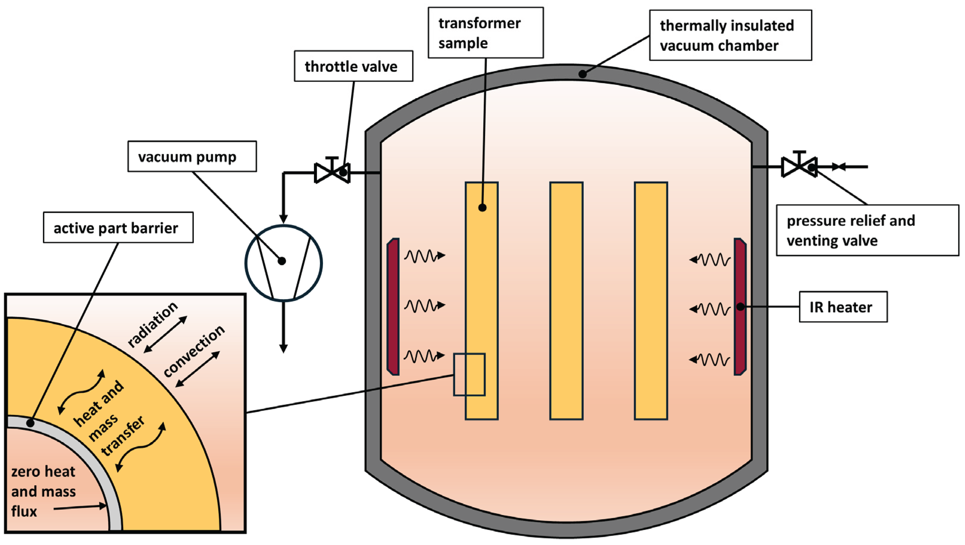
Figure 2.
Heat and mass transport mechanisms through cellulose insulation.
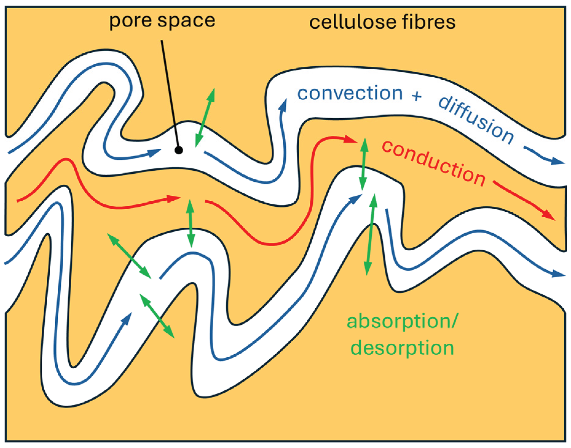
Figure 3.
GAB model equilibrium moisture content of the new Kraft paper (wireframe) and experimental values of moisture content (dots) [23].
Figure 3.
GAB model equilibrium moisture content of the new Kraft paper (wireframe) and experimental values of moisture content (dots) [23].
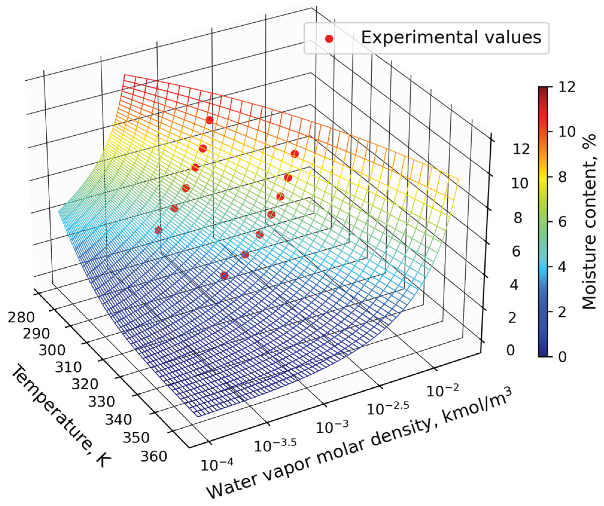
Figure 4.
Rudimentary geometry of the IR heaters, transformer samples and vacuum chamber generated with PyVista [33] package (used both in test case and drying case simulation)
Figure 4.
Rudimentary geometry of the IR heaters, transformer samples and vacuum chamber generated with PyVista [33] package (used both in test case and drying case simulation)
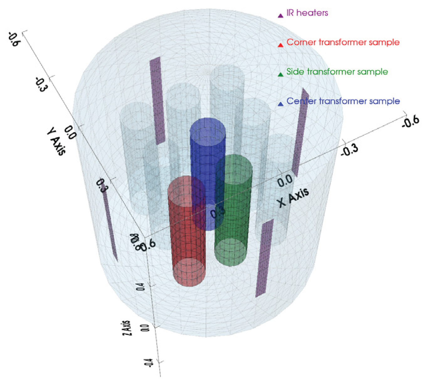
Figure 5.
Temporal variations of physical fields for each characteristic transformer sample ( m2, 1/s): (a) water vapor molar density, (b) dry air molar density, (c) temperature and (d) moisture content.
Figure 5.
Temporal variations of physical fields for each characteristic transformer sample ( m2, 1/s): (a) water vapor molar density, (b) dry air molar density, (c) temperature and (d) moisture content.
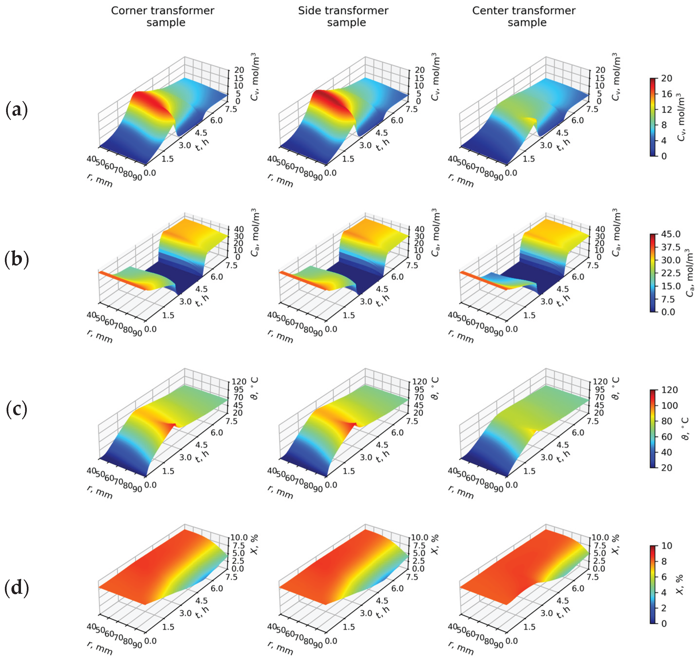
Figure 6.
Temporal variations of derived physical fields for each characteristic transformer sample ( m2, 1/s): (a) water vapor molar fraction, (b) absolute pressure.
Figure 6.
Temporal variations of derived physical fields for each characteristic transformer sample ( m2, 1/s): (a) water vapor molar fraction, (b) absolute pressure.
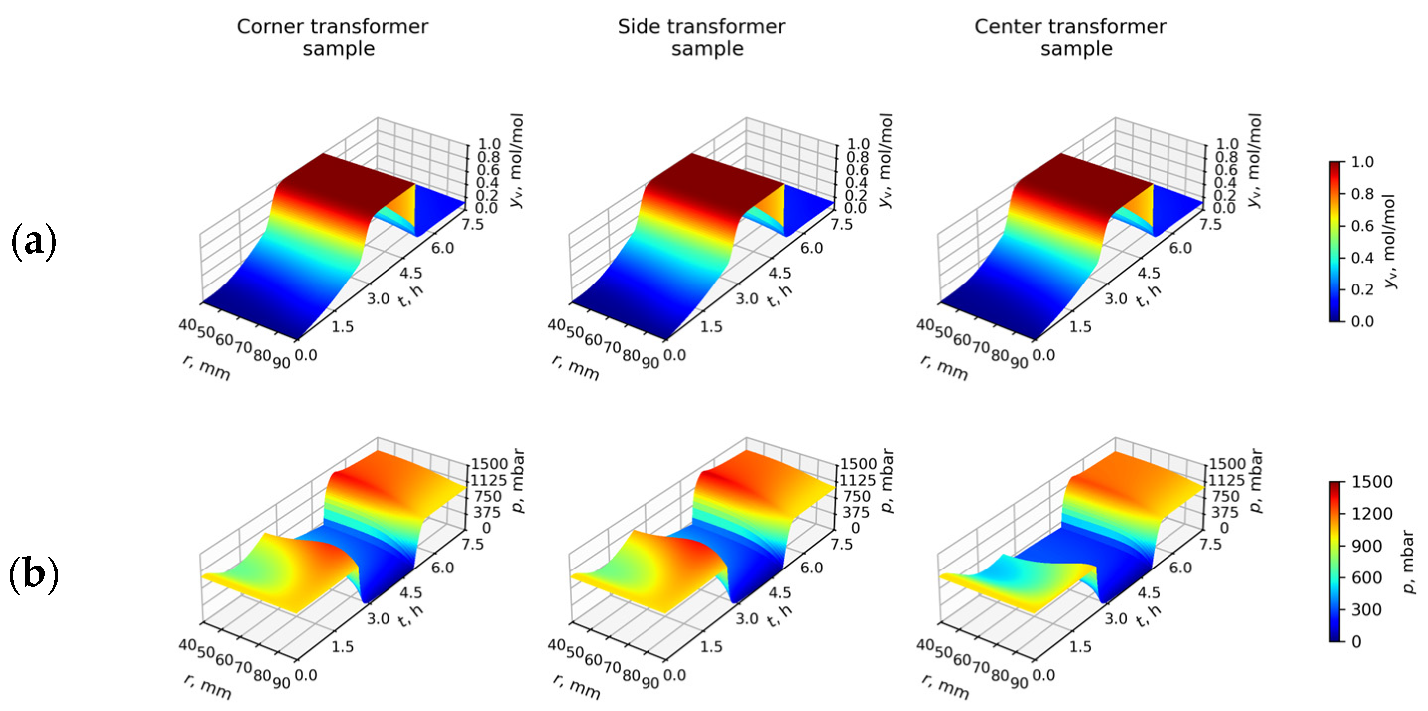
Figure 7.
Time-variations of the variables at the scale of the vacuum chamber ( m2, 1/s): (a) molar densities, pressure and water vapor molar fraction of the vacuum chamber atmosphere, (b) surface temperatures of the characteristic transformer samples, vacuum chamber atmosphere temperature, vacuum chamber walls temperature and IR heaters temperature (different scale on the right side).
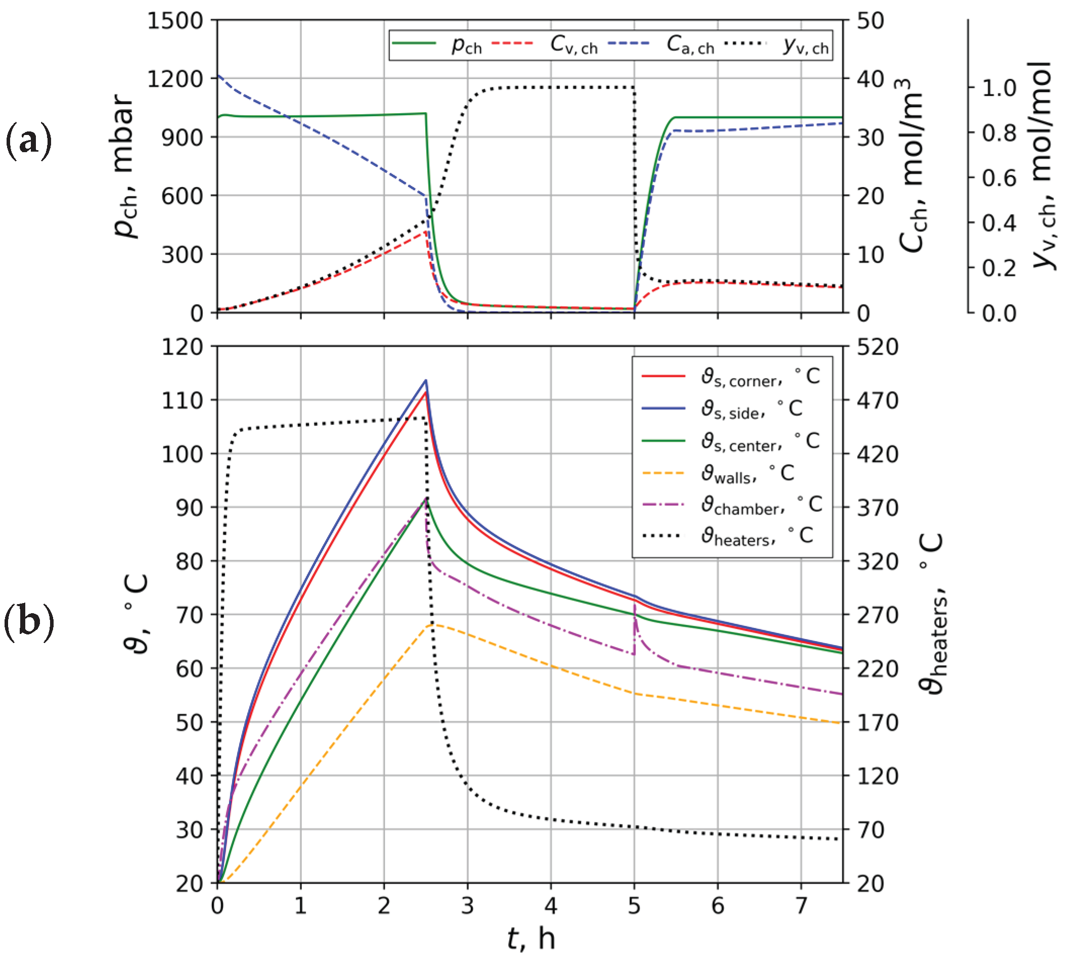
Figure 8.
Time-variations of the average moisture content of the cellulose insulation for the test case process: (a) influence of the overall internal mass transfer coefficient (with m2) and (b) influence of the absolute permeability (with 1/s).
Figure 8.
Time-variations of the average moisture content of the cellulose insulation for the test case process: (a) influence of the overall internal mass transfer coefficient (with m2) and (b) influence of the absolute permeability (with 1/s).
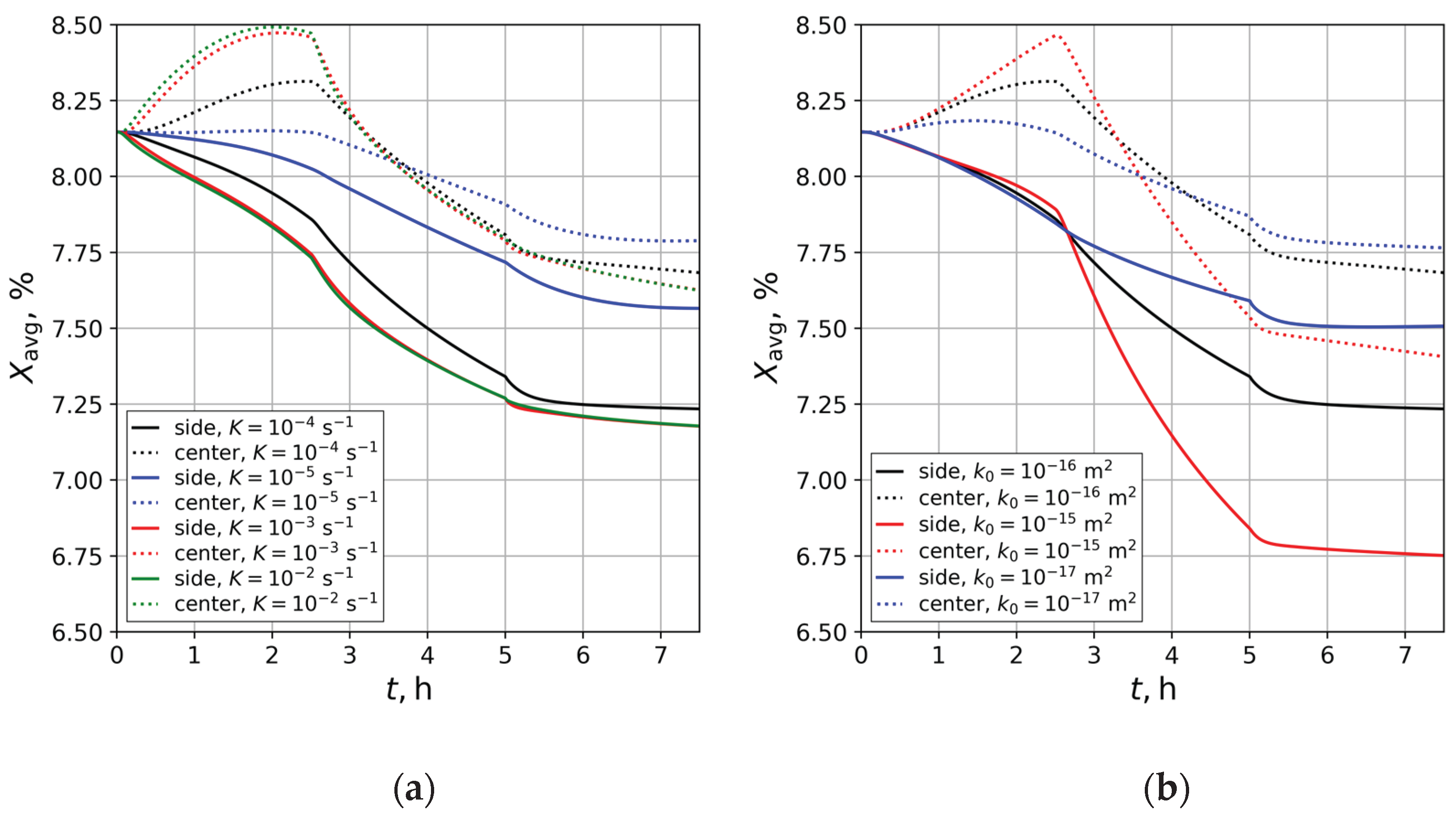
Figure 9.
Time-variations of the side and center transformer sample surface and innermost layer temperatures, along with the variation of pressure of the vacuum chamber atmosphere ( m2 and 1/s).
Figure 9.
Time-variations of the side and center transformer sample surface and innermost layer temperatures, along with the variation of pressure of the vacuum chamber atmosphere ( m2 and 1/s).
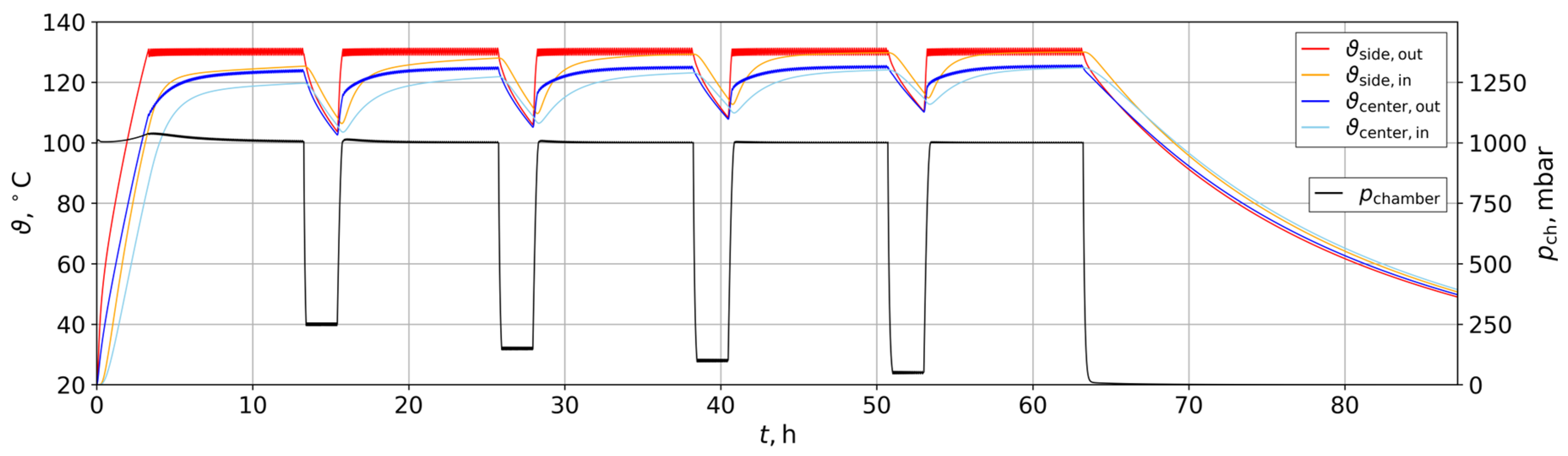
Figure 10.
Time-variations of the convective and radiative heat fluxes at the surface of the side and center transformer sample ( m2 and 1/s).
Figure 10.
Time-variations of the convective and radiative heat fluxes at the surface of the side and center transformer sample ( m2 and 1/s).
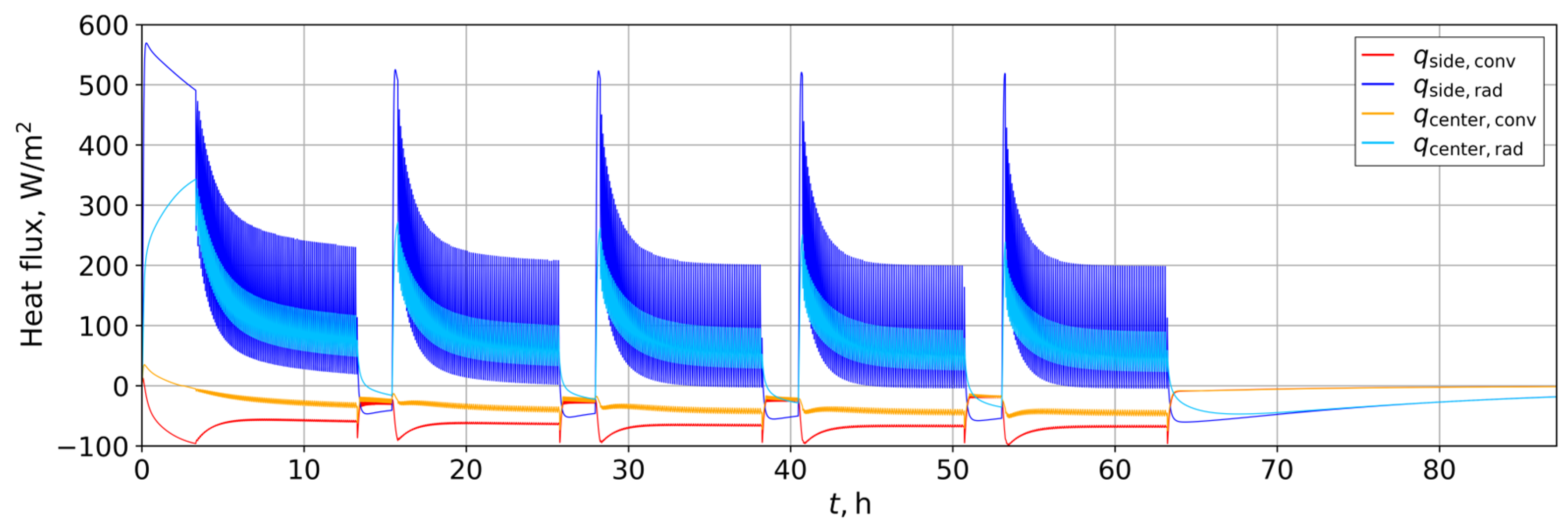
Figure 11.
Time variations ( m2 and 1/s) of the following quantities: (a) convective and diffusive molar flux at the surface of the side and center transformer sample, (b) drying rate of the side and center transformer samples, (c) drying curves of the corner, side and center transformer sample.
Figure 11.
Time variations ( m2 and 1/s) of the following quantities: (a) convective and diffusive molar flux at the surface of the side and center transformer sample, (b) drying rate of the side and center transformer samples, (c) drying curves of the corner, side and center transformer sample.
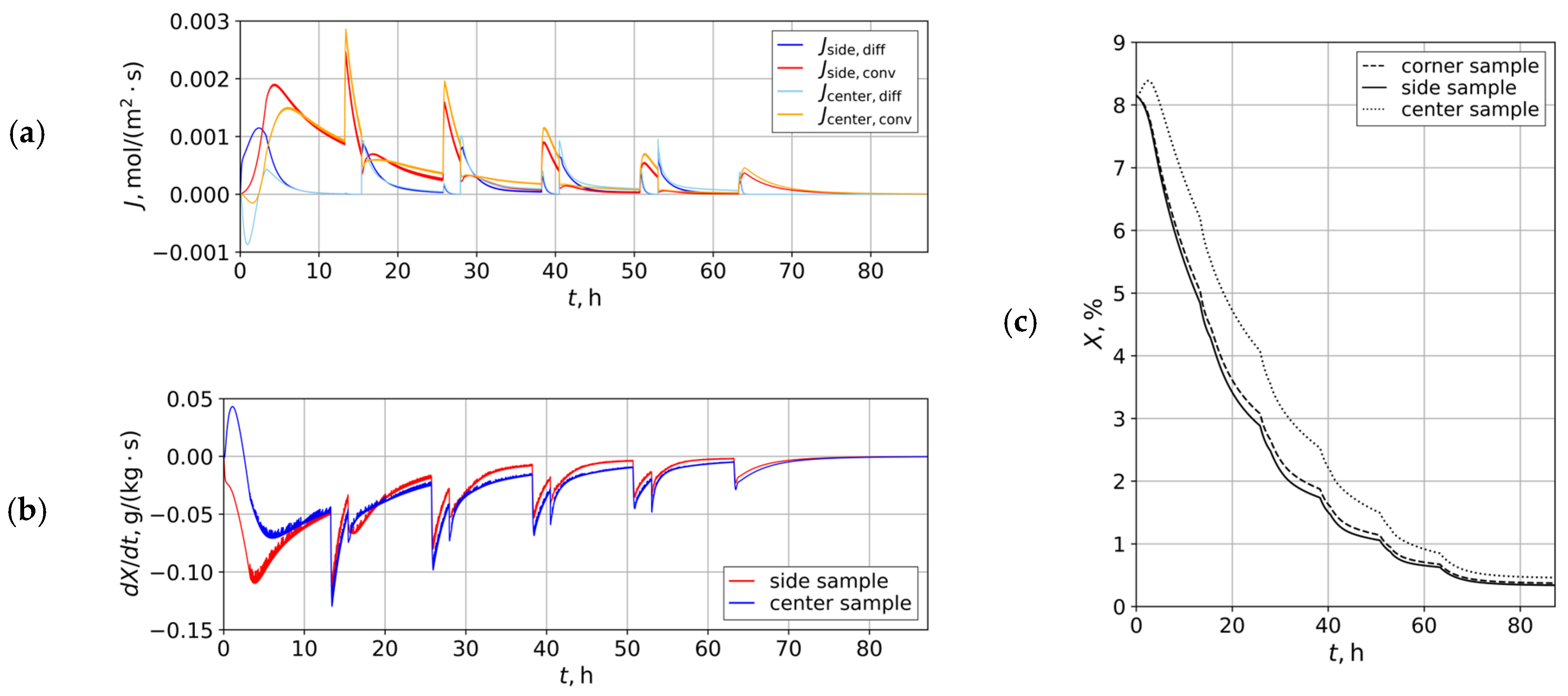
Table 1.
Calculated values of the view factors. Rows refer to the value of the view factor from surface marked in the index towards a surface marked on the top of the corresponding column
Table 1.
Calculated values of the view factors. Rows refer to the value of the view factor from surface marked in the index towards a surface marked on the top of the corresponding column
| View factor/ surface |
IR heaters | Vacuum chamber walls | Corner transformer sample |
Side transformer sample |
Center transformer sample |
|---|---|---|---|---|---|
| Fheaters - i | 0.0000 | 0.4102 | 0.2604 | 0.3295 | 0.0000 |
| Fwalls - i | 0.0098 | 0.7060 | 0.1533 | 0.1125 | 0.0183 |
| Fcorner t - i | 0.0271 | 0.6667 | 0.0000 | 0.2406 | 0.0657 |
| Fside t - i | 0.0343 | 0.4892 | 0.2406 | 0.1313 | 0.1046 |
| Fcenter t - i | 0.0000 | 0.3189 | 0.2626 | 0.4185 | 0.0000 |
Table 2.
Operational states of the main components and their durations governing the simulated test case.
Table 2.
Operational states of the main components and their durations governing the simulated test case.
| Order | Component status | Duration | ||
|---|---|---|---|---|
| IR heaters | Vacuum pump |
Venting/ pressure relief valve |
||
| 1 | on | off | on | 2.5 h |
| 2 | off | on | off | 2.5 h |
| 3 | off | off | on | 2.5 h |
Table 3.
Operational states of the main components and their durations governing the simulated drying case.
Table 3.
Operational states of the main components and their durations governing the simulated drying case.
| Order | Controlled variable |
Component status | Duration1 | ||
|---|---|---|---|---|---|
| IR heaters | Vacuum pump | Venting/ pressure relief valve |
|||
| 1 | 130 ± 1 ⁰C | on/off | off | on | 10 h |
| 2 | 25 ± 0.5 kPa | off | on/off | off | 2 h |
| 3 | 130 ± 1 ⁰C | on/off | off | on | 10 h |
| 4 | 15 ± 0.5 kPa | off | on/off | off | 2 h |
| 5 | 130 ± 1 ⁰C | on/off | off | on | 10 h |
| 6 | 10 ± 0.5 kPa | off | on/off | off | 2 h |
| 7 | 130 ± 1 ⁰C | on/off | off | on | 10 h |
| 8 | 5 ± 0.5 kPa | off | on/off | off | 2 h |
| 9 | 130 ± 1 ⁰C | on/off | off | on | 10 h |
| 10 | min. pressure | off | on | off | 30 h |
1 transient period durations are not included.
Disclaimer/Publisher’s Note: The statements, opinions and data contained in all publications are solely those of the individual author(s) and contributor(s) and not of MDPI and/or the editor(s). MDPI and/or the editor(s) disclaim responsibility for any injury to people or property resulting from any ideas, methods, instructions or products referred to in the content. |
© 2025 by the authors. Licensee MDPI, Basel, Switzerland. This article is an open access article distributed under the terms and conditions of the Creative Commons Attribution (CC BY) license (http://creativecommons.org/licenses/by/4.0/).
Copyright: This open access article is published under a Creative Commons CC BY 4.0 license, which permit the free download, distribution, and reuse, provided that the author and preprint are cited in any reuse.


