
Submitted:
23 July 2025
Posted:
25 July 2025
You are already at the latest version
Abstract
This paper explores the synergies between process mining and Data Envelopment Analysis (DEA) in business process management. Process mining offers insights into organizational workflows by analyzing event logs, while DEA provides a robust framework for efficiency assessment across diverse sectors. In the initial stage, hierarchical data analysis was conducted to construct process information diagrams and categorize process traces based on various factors, including decision points for each case. In the second stage, process analysis concepts and process discovery algorithms were utilized to define and compute key performance indicators (KPIs) from the perspectives of organizational resources and individual cases, followed by constructing process diagrams using Alpha, Inductive, and Heuristic miners. In the third stage, a scenario-based robust DEA model was applied to rank the KPIs of employees derived from the event log data. Furthermore, we examine how the proposed scenario-based Robust DEA revolutionizes efficiency assessment, providing decision-makers with a comprehensive framework for evaluating organizational performance. Ultimately, by integrating ML prediction and behavior analysis, organizations can anticipate future trends, optimize operations, and drive continuous improvement. Ultimately, process mining and DEA represent indispensable tools for organizations seeking to enhance operational efficiency, mitigate risks, and achieve strategic objectives in today's dynamic business environment. The findings demonstrate that this comprehensive integration of techniques provides profound insights into the event logs, identifying strengths, weaknesses, bottlenecks, and overall system efficiency, thereby facilitating organizational improvement and optimization.
Keywords:
process mining
; data envelopment analysis
; robust optimization
; prediction
; behavior analysis
1. Introduction
In today’s dynamic business environment, organizations constantly seek ways to enhance operational efficiency, mitigate risks, and achieve strategic objectives (Hammer, 2010). One of the critical challenges decision-makers face is the lack of comprehensive and actionable insights into their business processes (Dumas et al., 2018). Business processes are typically complex and multifaceted, involving numerous decision points, interactions, and dependencies (Dumas et al., 2018). As organizations grow, these processes become even more intricate, making it increasingly challenging to identify inefficiencies, bottlenecks, and areas for improvement (Van der Alast, 2016). Conventional approaches to process analysis and efficiency assessment often rely on isolated metrics and static models, which fail to provide a holistic view of the organization’s performance (Hammer, 2010). This fragmentation hinders the ability to drive continuous improvement and achieve strategic goals. Therefore, traditional efficiency assessment methods often fall short of capturing the complexities and variances inherent in organizational workflows, leading to suboptimal decision-making and resource allocation (Harmon, 2014).
This paper explores the synergies between process mining and DEA1 to address the limitations of traditional efficiency assessment methods in business process management. Process mining leverages event log data to uncover detailed insights into organizational workflows, revealing patterns, deviations, and performance issues (Van der Alast, et al., 2005). On the other hand, DEA offers a robust quantitative framework for evaluating the relative efficiency of decision-making units (DMUs) across various sectors (Cooper et al., 2007). We demonstrate how insights gained from analyzing the BPI 2012 dataset can optimize loan application processes or similar processes in other organizations. This paper includes modifications, reviews, and extensions of previous findings and articles in the process mining domain, precisely the BPI 2012 challenge. The innovations of the article are as follows:
- Providing a segmentation strategy that separates the process into manageable sub-stages for separate analysis.
- Overall analysis of recorded event logs and organizational resources or staff involved in the lending process.
- Identifying bottlenecks, deviations, and areas for improvement through process analysis.
- The paper extracts KPIs from the perspectives of organizational resources and individual cases, using Alpha, Inductive, and Heuristic miners to construct process diagrams.
- These KPIs are then evaluated using a scenario-based robust DEA model to rank the performance of employees, providing a robust framework for resource performance assessment and optimization.
- The study integrates machine learning prediction and behavior analysis to anticipate future trends, optimize operations, and drive continuous improvement.
This paper underscores the dynamic nature of process mining and its application in real-world scenarios. It showcases the continuous development of techniques and methods to derive valuable insights from event data. This critical aspect keeps the reader updated on the latest advancements in the field. It also underscores the importance of selecting appropriate event logs to improve process discovery and solve issues to enhance the effectiveness of process mining.
2. Literature Review
2.1. Process Mining
Process mining, a pivotal discipline within business process management, offers profound insights into organizational workflows by analyzing event logs.
2.1.1. Foundational Concepts and Techniques
A seminal paper by van der Aalst et al. (2011) lays the groundwork for understanding the core concepts of process mining, introducing fundamental techniques such as process discovery, conformance checking, and process enhancement. This foundational work provides researchers and practitioners with essential methodologies for understanding and improving business processes. Van der Aalst (2016) further expands on these concepts in his comprehensive book, “Process Mining: Discovery, Conformance and Enhancement of Business Processes.” This seminal publication delves into various process mining techniques, including process discovery algorithms, conformance-checking strategies, and process enhancement methodologies. It serves as an indispensable guide for both novice and seasoned professionals seeking to leverage process mining in their organizational contexts. Building upon theoretical frameworks, van der Aalst (2016) also provides practical insights into applying process mining techniques in real-world scenarios. His book, “Process Mining: Data Science in Action,” presents case studies and examples illustrating how process mining can drive operational efficiency, identify bottlenecks, and optimize business processes. This bridge between theory and practice enhances the accessibility and applicability of process mining methodologies across diverse industries.
2.1.2. Practical Tools and Implementation
In addition to theoretical advancements, practical tools play a crucial role in the adoption and implementation of process mining techniques. The ProM toolkit, introduced by van Dongen et al. (2005), stands out as an open-source framework for process mining analysis. This toolkit facilitates various process mining tasks, including event log analysis and process model visualization, thus empowering researchers and practitioners to explore and analyze their data effectively. Maruster and Van der Aalst (2013) provide a systematic approach for selecting accurate event logs, a crucial step in conducting process mining analyses. They address the challenges and considerations of obtaining appropriate datasets for process analysis. The authors discuss the importance of selecting relevant logs to ensure process mining results align with real-world scenarios. This work elucidates the practical aspects of data collection, which is fundamental to process mining. Weijters and Ribeiro (2013) introduce the Flexible Heuristics Miner (FHM), a novel approach developed for the BPI 2012 competition. The authors highlight the significance of process discovery as a fundamental step in process mining and detail the performance of the FHM algorithm. This work advances process discovery methods, making them more flexible and adaptable to various types of event data. Weijters and Ribeiro (2014) present a tree-based approach for analyzing collaborative business processes. This approach helps understand complex, collaborative workflows. The authors propose a tree-based representation of processes, which can benefit scenarios involving multiple parties in process execution, such as supply chain management or interdepartmental workflows.
2.1.3. Ethical Considerations and Collaborative Efforts
Ethical considerations and collaborative efforts are paramount in advancing the field of process mining. Van der Aalst et al. (2011) outline principles and challenges in process mining research and practice, emphasizing the importance of transparency, reproducibility, and responsible data usage. This manifesto serves as a guiding framework for stakeholders to navigate the evolving landscape of process mining while ensuring ethical standards and responsible conduct.
2.2. Business Process Mining – BPI Challenge 2012
Process mining has emerged as a vital tool for analyzing and optimizing business processes, offering insights into organizational workflows through the analysis of event data. The Business Process Intelligence (BPI) Challenge 2012 is pivotal, providing researchers and practitioners with real-world datasets and challenges to advance process mining methodologies. The BPI Challenge 2012 introduced a dataset of event logs from a real-life process involving insurance claims handling. This dataset was the foundation for numerous academic papers, providing researchers with a standardized benchmark for evaluating and comparing process mining techniques. A seminal paper by van der Aalst et al. (2012) provides an overview of the challenge, including the dataset, evaluation criteria, and results, establishing a common reference point for subsequent research endeavors. Building upon the BPI Challenge 2012 dataset, researchers have explored various process mining techniques to uncover insights and address challenges inherent in business operations. Leemans et al. (2013) proposed an approach for efficiently mining generalized association rules from event logs, demonstrating how these rules can reveal behavior patterns and identify potential bottlenecks. This research sheds light on the practical applications of process mining in identifying process inefficiencies and driving operational improvements. Carmona et al. (2018) reviewed automated process discovery techniques comprehensively, benchmarking various algorithms using the BPI Challenge 2012 dataset. Their analysis provides valuable insights into the strengths and limitations of existing process discovery techniques, offering guidance for researchers and practitioners in selecting appropriate methodologies for analyzing event data. This research contributes to the ongoing refinement and development of process mining techniques tailored to business contexts. While the BPI Challenge 2012 dataset has been instrumental in advancing process mining research, it is also part of a broader academic discourse on process discovery and analysis. Adriansyah et al. (2011) conducted a literature survey on process discovery techniques, providing a comprehensive overview of algorithms and methodologies for analyzing event data. Although not directly focused on the BPI Challenge 2012 dataset, their review offers valuable insights into process mining techniques’ theoretical foundations and practical applications.
2.3. Data Envelopment Analysis
Data Envelopment Analysis (DEA) is a linear programming-based technique used for measuring the relative performance efficiency of decision-making units (DMUs) in the presence of multiple inputs and outputs (Thanassoulis, 2001). These DMUs can be departments, companies, or organizational entities that convert inputs into outputs. DEA helps organizations evaluate their performance by comparing them with peers or best-practice benchmarks (Cooper et al., 2007). Subsequent works extended DEA, addressing issues like scale efficiency and theoretical foundations. Charnes, Cooper, Seiford, and Stutz (1983) introduced invariant multiplicative efficiency, while their 1985 paper explored DEA’s theoretical underpinnings. These papers have been instrumental in DEA’s application across fields, offering essential methodologies and insights for efficiency analysis. In their comprehensive Charnes, Cooper, Golany, Seiford, and Stutz (1985) delved into the theoretical foundations of DEA. Focusing on Pareto-Koopmans efficient empirical production functions, they explored the mathematical underpinnings of DEA models and their relationship to classical production theory. By elucidating the theoretical basis of DEA, this paper provided valuable insights into its application and interpretation in empirical settings.
2.4. Robust Scenario-Based Data Envelopment Analysis
Robust optimization, a methodology designed to develop solutions that can withstand uncertainties, has proven effective in various real-world scenarios. Mulvey, Vanderbei, and Zenios (1995) pioneered this concept, providing mathematical formulations for large-scale problems. Leung et al. (2007) demonstrated its practical application in multi-site production planning, further solidifying its relevance. Other key works, such as Ben-Tal and Nemirovski’s (2009) comprehensive overview and Bertsimas and Sim’s (2004) insights into practical implementation, have contributed to the robust optimization’s status as a crucial tool for decision-makers navigating uncertainties in diverse domains.
Robust Data Envelopment Analysis (DEA) methodology addresses uncertainties and variations in data, ensuring reliable efficiency assessments in real-world scenarios. Inspired by Mulvey, Vanderbei, and Zenios (1995), who introduced robust optimization of large-scale systems, and Leung, Tsang, Ng, and Wu (2007), who proposed a robust optimization model for multi-site production planning, robust DEA extends traditional DEA to handle uncertain inputs, outputs, and environmental conditions. Robust DEA offers more resilient decision-making frameworks for complex systems like healthcare, finance, and manufacturing by integrating uncertainty into the efficiency evaluation. This approach enhances the decision-makers ability to assess and improve operational efficiency under dynamic and uncertain conditions, ultimately leading to more informed and robust management strategies.
2.5. Supervised Learning
2.5.1. Artificial Neural Networks (ANN)
Artificial Neural Networks have been extensively studied since their inception in the 1940s. The resurgence of interest in ANNs, particularly in deep learning, can be attributed to advances in computational power and the availability of large datasets. ANNs have demonstrated remarkable success in tasks such as image and speech recognition, natural language processing, and autonomous driving (LeCun et al., 2015). Researchers like LeCun, Bengio, and Hinton (2015) have highlighted the capabilities of deep learning, a subset of ANNs, in their seminal work. They discuss the architecture of deep neural networks, which include convolutional neural networks (CNNs) and recurrent neural networks (RNNs), and their applications in various fields. The backpropagation algorithm, introduced by Rumelhart, Hinton, and Williams (1986), remains a fundamental component for training these networks by minimizing the loss function through gradient descent.
2.5.2. K-Nearest Neighbors (KNN)
The k-Nearest Neighbors algorithm, first introduced by Fix and Hodges in 1951, has retained its popularity due to its intuitive approach and ease of implementation. KNN is a non-parametric method, making no assumptions about the underlying data distribution. This characteristic makes it remarkably versatile for various applications, including pattern recognition, data mining, and intrusion detection systems (Cover & Hart, 1967). Research by Cover and Hart (1967) formalized the theoretical foundation of KNN and proved its effectiveness in classification tasks. More recent studies, such as those by Altman (1992), have explored enhancements to the basic KNN algorithm, including weighted KNN and using distance metrics like Euclidean and Manhattan distances to improve performance.
2.5.3. Gradient Boosting (GB)
Gradient Boosting has emerged as a powerful ensemble technique, particularly in structured data problems. (Friedman, 2001) introduced the methodology and demonstrated its efficacy in regression and classification tasks. Gradient Boosting works by sequentially adding models that correct the errors of the previous models, thus creating a robust predictive model from several weak learners. The advent of XGBoost, developed by Chen and Guestrin (2016), has further popularized gradient boosting due to its superior performance and scalability. XGBoost has been widely adopted in various machine-learning competitions and real-world applications, proving its robustness and efficiency. Recent advancements have focused on improving the interpretability and reducing the computational complexity of gradient-boosting models.
Comparing ANN, KNN, and GB reveals distinct strengths and weaknesses. ANNs excel in tasks involving large amounts of unstructured data, such as images and text, due to their ability to learn complex representations (LeCun et al., 2015). However, they require significant computational resources and large datasets for training (Rumelhart et al., 1986). KNN, conversely, is simple to implement and effective for small datasets but can be computationally expensive for large datasets due to its reliance on distance calculations (Cover & Hart, 1967). Gradient Boosting strikes a balance by providing high predictive accuracy and handling structured data efficiently (Friedman, 2001). However, it can be prone to overfitting and may require careful tuning of hyperparameters (Chen & Guestrin, 2016). Each of these algorithms has its place in the machine learning toolbox, and their applicability depends on the specific requirements of the task at hand.
2.5.4. Long Short-Term Memory (LSTM) Networks
Long Short-Term Memory networks have been extensively studied since their introduction by Hochreiter and Schmidhuber in 1997. The primary motivation behind LSTMs was to overcome the difficulties standard RNNs face in learning long-term dependencies. LSTMs introduce a unique cell structure with gates—input, output, and forget gates—that regulate the flow of information, enabling the network to maintain and update memory over extended sequences (Hochreiter & Schmidhuber, 1997). LSTMs have demonstrated remarkable success in various sequential tasks. For instance, Graves et al. (2013) showcased the potential of LSTMs in speech recognition, while Sutskever et al. (2014) highlighted their efficacy in sequence-to-sequence learning, particularly in machine translation. These studies underscore the versatility and robustness of LSTM networks in handling diverse sequential data challenges.
2.5.6. Predicting Next Activity
Predicting the next activity involves anticipating future actions based on historical sequences. This is particularly relevant in fields such as human activity recognition, where accurate prediction models can enhance applications like healthcare monitoring, smart home automation, and personalized services. One notable application of LSTMs in activity prediction is process mining, where LSTM models predict the next event in business process logs. Tax et al. (2017) demonstrated the effectiveness of LSTMs in predicting the next activity in business processes, highlighting their ability to capture complex temporal dependencies and improve predictive accuracy.
Comparing LSTM models with other machine learning approaches reveals distinct strengths and weaknesses. LSTMs excel in tasks involving long-term dependencies and sequential data, making them suitable for time series forecasting and activity prediction. However, they require significant computational resources and large datasets for training (Hochreiter & Schmidhuber, 1997). Traditional machine learning algorithms, such as decision trees or support vector machines, may struggle to capture temporal dynamics effectively. On the other hand, simple RNNs, while capable of handling sequential data, often fall short of maintaining long-term dependencies due to gradient-related issues. LSTMs address these limitations by incorporating memory cells and gates that enhance their ability to learn and remember essential patterns over extended sequences (Graves et al., 2013).
2.6. Behavior Analysis
A diverse range of models exist in customer behavior modeling, each offering unique advantages depending on the specific dataset and use case. Understanding customer purchase patterns and forecasting future behaviors is crucial for businesses to optimize marketing strategies, improve customer retention, and enhance overall profitability. This research’s significance lies in its potential to guide practitioners in selecting the most appropriate model for their specific needs, thereby maximizing the accuracy and efficiency of their predictions. Starting from the foundational NBD model proposed by Ehrenberg in 1959, which serves as a fundamental benchmark, the evolution of buy-till-you-die models has been substantial. The Pareto/NBD model, introduced in 1987, remains a gold standard due to its combination of transaction and dropout processes. The BG/NBD model, proposed by (Batislam et al., 2007) and (Hoppe & Wagner, 2007), modifies these assumptions to enhance computational efficiency and robustness.
Further improvements led to the MBG/NBD model, addressing inconsistencies in dropout assumptions by allowing customers without repeat transactions to remain inactive, as (Reutterer et al.., 2020) detailed. Recent advancements include the BG/CNBD-k and MBG/CNBD-k models, which incorporate regularity in transaction timings and substantially improve forecasting accuracy while maintaining similar computational costs. Models utilizing Markov-Chain-Monte-Carlo (MCMC) simulation, such as the hierarchical Bayes variant of Pareto/NBD by Ma and Liu (2007) and the Pareto/NBD (Abe) by Abe (2009), allow for more flexible assumptions and provide marginal posterior distributions and individual-level parameter estimates. The Pareto/GGG model, proposed by (Platzer & Reutterer, 2016), further generalizes the Pareto/NBD by accounting for varying transaction regularity, yielding significant forecasting accuracy improvements if such regularity exists in the data. While these models have traditionally been used to analyze customer behavior, they can also be applied to analyze the behavior of resources, such as those in an event log. By accurately predicting resource efficiency, these models can inform data envelopment analysis (DEA) models, particularly when incorporating uncertainty. Evaluating each model’s data fit, forecast accuracy, and computational efficiency for resource behavior prediction allows for selecting the best model, which can then be integrated into the DEA framework to predict future resource efficiency effectively. Given the array of models available, practitioners should evaluate each model’s data fit, forecast accuracy, and computational efficiency for their specific datasets, making informed trade-offs to identify the most suitable approach. This comprehensive review and comparison of various customer behavior models highlight the continuous advancements in this field and underscore the importance of selecting the suitable model to enhance business decision-making.
3. Materials and Methods
The insights gained from process mining were integrated with the DEA results to analyze process performance comprehensively. This integrated approach facilitated the identification of bottlenecks, inefficiencies, and areas of non-compliance within the processes. Visualization tools were used to create process diagrams and efficiency scores, making understanding and communicating the findings easier. This holistic analysis helped pinpoint weak and strong points within the organization, guiding targeted improvements to enhance overall process efficiency and effectiveness. A scenario-based robust DEA model was employed to evaluate and rank the efficiency of organizational resources. This involved defining input and output variables, where inputs included resources such as work-related and process-related ones, and outputs consisted of processed cases and compliance rates. The DEA model provided efficiency scores for each decision-making unit (DMU), highlighting areas for improvement and allowing for a comparative analysis of resource utilization across different units. This paper proposes a robust DEA model for calculating efficiency for a Dutch financial institute by determining common weights for all inputs and output parameters under uncertain conditions. The introduced model is based on a robust optimization approach proposed by (Mulvey et al., 1995). Moreover, later modified by (Leung et al., 2007), it could be considered a superior alternative to sensitivity analysis for dealing with imprecise data.
3.1. Data Collection and Preparation
The study utilized event log data from the BPI 2012 challenge, sourced from a Dutch financial institute. This dataset included detailed records of the financial processes, capturing various attributes such as timestamps, activities, and resources involved. Initial data cleaning was performed to handle missing values, remove noise, and ensure log consistency. This process involved filtering out incomplete cases and standardizing the format of data entries to ensure they were suitable for further analysis. The event logs were then segmented based on several criteria, including decision points, timestamps, and resource allocations, to facilitate a hierarchical analysis of the processes.
3.2. Process Mining Techniques
A multi-level approach was employed to track and plot process information diagrams, providing a comprehensive workflow view. The process traces were divided according to decision points and specific case characteristics. Three process discovery algorithms were utilized to uncover the underlying structure of the processes. The Alpha Miner was applied to discover the basic structure of the processes. At the same time, the Inductive Miner was chosen for its ability to handle noise and incompleteness in the logs, resulting in a more accurate process model. The Heuristic Miner was used to analyze complex relationships and dependencies within the processes, providing deeper insights into the process dynamics.
| Algorithm 1 IM Algorithm |
|
1. For each activity in activities, do: 2. Compute the connected activities of a distinct, unrelated group G 3. If the length of any connected activities in G is greater than one, then: 4. Return the connected activities as a cut partition 5. End if 6. End for. 7. For each activity in activities, do: 8. Given a set of activities, A: 9. Classify activities into groups such that each group has a start and end activity, and the activities between them directly follow relations 10. Partition A into groups {P1,…., Pn} such that there are no pairwise reachable activities in different groups 11. Merge the pairwise unreachable activities to create the final groups {P1,…., Pn} 12. Order the resulting groups 13. If {n > 1} then: 14. Return {P1,…., Pn } as a cut partition 15. End if 16. End for 17. For each activity in `activities` do: 18. Given a set of activities A: 19. For each group G do: 20. If G does not have a start or end activity, then: 21. Merge G with another arbitrary group 22. End if 23. End for 24. Partition the resulting sub-groups 25. If the partition has a length greater than one, then: 26. Return the resulting partition as a cut partition 27. End if 28. End for 29. For each activity in `activities` do: 30. P1 set of all start and end activities in L 31. {P2,…., Pn} partition of all other activities in L such that with Pi and β ∈ Pj implies i< j 32. For i ←2 to n do: 33. If Pi is connected to P1 through a start or end activity, then: 34. Merge Pi with P1 35. Else if Pi has an activity connected to some but not all start activities of P1, then: 36. Merge Pi with P1 37. Else if Pi has an activity connected from some but not all end activities of P1, then: 38. Merge Pi with P1 39. End if 40. End for 41. If {n > 1} then: 42. Return {P1,…., Pn} as cut partition 43. End if 44. End for |
| Algorithm 2 HM Algorithm |
|
1. Initialize empty set A of candidate activities 2. Initialize empty set S of candidate sequences 3. Initialize empty process model M 4. For each trace t in L, do: 5. For each activity a in t do: 6. Add a to A 7. End for. 8. For i from 1 to length(t) - 1 do: 9. For j from i + 1 to length(t) do: 10. s ← sequence of activities from ti to tj 11. Add s to S 12. End for 13. End for 14. End for 15. For each candidate sequence s in S, do: 16. count ← frequency of s in L 17. If count f then: 18. Add s to M 19. End if 20. End for 21. Refine M using optimization heuristics 22. Return M |
3.3. Data Envelopment Analysis (DEA)
The DEA model proposed by (Charnes et al., 1978):
Model (1) is initially formulated as a non-linear programming problem, requiring implementation n times to assess the relative efficiency of all Decision-Making Units (DMUs). The Charnes, Cooper, and Rhodes (CCR) model plays a foundational role in the (Charnes et al., 1985) by establishing the method for evaluating the efficiency of decision-making units (DMUs):
Model (2) is a method for constructing and analyzing Pareto-efficient frontier production functions using Data Envelopment Analysis (DEA). The dual of Model (2) is presented in Model (3) as follows:
Unlike Model (3), which needs to be run n times to calculate individual weights for each input and output, Model (4) must be solved only once to calculate standard weights for all inputs and outputs. This makes it less computationally intensive. In this new approach, the objective function aims to maximize the summation of all DMUs’ efficiency.
To prevent assigning zero values to weights, we assume that all weights are greater than or equal to a minimal value, epsilon ().
3.4. Robust Optimizations
Scenario-based robust optimization is a technique for solving optimization problems under uncertainty. It involves formulating the problem using a set of possible scenarios, each with an associated probability of occurrence. The goal is to find a robust solution that performs well across multiple scenarios while minimizing a measure of infeasibility.
(Mulvey et al., 1995) suggested robust optimization, which provides risk-averse solutions less sensitive to fluctuations in data across scenarios, to handle data uncertainty. It captures potential values for diverse circumstances using discrete scenarios to ascertain unclear parameters. The goal is to arrive at a solution that is consistent in all circumstances, complies with the preferences of a predetermined decision-maker, and is versatile in real-world situations.
Let Be vectors of design variables and Vectors of control variables. The general notation and formulation are as follows:
The first constraint is related to structural and certain, but the second constraint describes control variables and varies in different scenarios, Are our scenarios. Coefficient control depends on each scenario, and index s is assigned to them. . Each scenario is fixed with probability. where . The robust optimization model aims to balance solution robustness and model robustness. Solution robustness refers to the optimal solution remaining close to optimality across scenarios, while model robustness indicates the solution remaining almost feasible for various scenarios. However, the model may not simultaneously provide optimal and feasible solutions for all scenarios under specific conditions. Hence, a trade-off between solution and model robustness is crucial in robust optimization. This trade-off is quantified through the robust optimization model formulation.
The robust optimization model is formulated as follows:
The first term in Model (6) calculates the optimality robustness as the mean value of plus a constraint Times the variance:
The second term measures the model’s robustness besides the feasibility penalty function, which calculates the legal exceeding of each control constraint. Equation (7) is in quadratic form so (Leung et al., 2007) convert it to non-quadratic form in Model (8):
It is evident that if then so in the second possible outcome then and so .

Table 1.
Notations.
| Indices |
|
Parameters Parameters |
3.5. Robust Optimization DEA
Our DEA model that contains uncertain factors is:
Finally, the proposed model is described as Model (11):
Model (11) is single objective linear programming that can be adequately solved.
3.6. Prediction
Artificial Intelligence (AI) and Machine Learning (ML) have revolutionized various sectors by enabling data-driven decision-making and predictive analytics. Among the plethora of algorithms available in the machine learning domain, Artificial Neural Networks (ANN), k-nearest Neighbors (KNN), Gradient Boosting (GB), and Long Short-Term Memory (LSTM) networks stand out due to their distinct characteristics and versatile applications. These algorithms have been widely researched and applied across numerous fields, from healthcare and finance to image and speech recognition. Specifically, LSTMs, a recurrent neural network (RNN), excel in capturing temporal dependencies and sequence patterns, making them particularly effective for tasks involving sequential data, such as time series forecasting, speech recognition, and predictive maintenance.
3.6.1. Loan Receiving Prediction
In the financial sector, these algorithms’ critical applications predict loan acquisition or rejection based on extracted Key Performance Indicators (KPIs). Accurate prediction models can significantly enhance decision-making processes in lending institutions, reduce default rates, and improve customer satisfaction by streamlining the loan approval process.
Artificial Neural Networks (ANN) are inspired by the biological neural networks that constitute human brains. They are designed to recognize patterns, classify data, and make predictions by learning from examples. ANNs consist of layers of interconnected nodes, or neurons, where each connection represents a weighted value. Through learning, ANNs adjust these weights to minimize error and improve accuracy (LeCun et al., 2015). This capability makes them highly effective in handling complex and non-linear data relationships often present in financial datasets.
The k-Nearest Neighbors (KNN) algorithm is a simple yet powerful supervised learning method. It classifies a data point based on how its neighbors are classified. KNN makes predictions by finding the ‘k’ most similar data points (neighbors) and using their values to determine the output. This algorithm is beneficial for classification tasks and is appreciated for its simplicity and effectiveness in handling non-linear data (Cover & Hart, 1967). In the context of loan approval, KNN can be employed to identify patterns in historical loan data and classify new loan applications accordingly.
Gradient Boosting (GB) is an ensemble learning technique that builds models sequentially, with each new model attempting to correct errors made by the previous ones. This iterative process involves training weak learners, usually decision trees, and combining them to form a robust predictive model. Gradient Boosting is known for its robustness and high predictive performance, especially in complex data structures (Friedman, 2001). Its ability to handle various data types and mitigate overfitting makes it an excellent choice for financial prediction tasks.
This part aims to comprehensively review these three machine learning algorithms: ANN, KNN, and GB. It explores their theoretical foundations, practical applications, and comparative performance in various domains, explicitly focusing on their application in predicting loan acquisition or rejection based on KPIs. By examining the strengths and limitations of each algorithm, this study seeks to offer insights into their appropriate usage and potential for future research.
3.6.2. Next Activity Prediction
LSTM models have shown significant promise in predicting the next activity. Accurate activity prediction models can enhance decision-making processes in numerous applications, including human activity recognition, process mining, and user behavior analysis. By anticipating future actions based on historical data, these models can provide valuable insights, improve operational efficiency, and enhance user experience. Long-short-term memory (LSTM) networks are designed to address the limitations of traditional RNNs, precisely their inability to handle long-term dependencies due to issues like vanishing and exploding gradients. LSTMs incorporate memory cells that can maintain information over long periods, allowing the network to learn and remember critical temporal patterns. This makes LSTMs highly effective in capturing the sequential dynamics inherent in activity prediction tasks.
3.7. Behavior Analysis
This section’s steps are as follows:
- 1)
- Model Selection: Choose a range of customer behavior models, including NBD, Pareto/NBD, BG/NBD, MBG/NBD, BG/CNBD-k, MBG/CNBD-k, hierarchical Bayes variant of Pareto/NBD, Pareto/NBD (Abe), and Pareto/GGG.
- 2)
- Dataset Preparation: To test the models, collect and prepare datasets reflecting various customer behaviors and resource usage patterns (extracted KPIs).
- 3)
- Model Implementation: Implement and calibrate each model to fit the prepared datasets, adjusting for specific dataset characteristics.
- 4)
- Performance Evaluation: Evaluate model performance using metrics such as Log-likelihood and mean error.
- 5)
- Comparative Analysis: Compare the models based on performance metrics to identify their strengths, weaknesses, and optimal use cases.
- 6)
- Integration with DEA: Incorporate the best-performing models into the DEA framework to predict future resource efficiency, adjust for uncertainty, and validate effectiveness.
3.8. Tools and Software
Several tools and software were utilized throughout the study. Python was used for process mining and discovery algorithms, process visualization, and performance analysis. The GAMS Solver was used to implement and solve the robust DEA models. Additionally, Python and R scripts were developed for data cleaning, pre-processing, and KPI calculations, ensuring a thorough and systematic approach to the analysis.
4. Results and Discussions
In this section, the research findings are reported. Tables, Figures, and the presentation of statistics in Persian, including the description and analysis of the data, should accompany the findings. The event log data includes 13,087 loan or overdraft requests and a total of 262,200 events over approximately six months from October 2011 to March 2012, starting with submitting the request by the applicant and ultimately ending in either approval, cancellation, or rejection. Each case includes an attribute called AMOUNT_REQ, which indicates the requested loan amount. For each event, the cycle includes the scheduling, start, completion, resource, and event time recorded according to its states.
4.1. Event Log Data Analysis
The primary language of the event log report is Dutch. Therefore, we introduce the profiles in the event log report provided in Table 2.
In examining the missing links between the start and complete events of activities where both events were discovered, we ultimately assess whether each instance of the complete event type has a corresponding start event. In the event log report, six activities have both start and complete event types. Table 3 shows the number of instances of such missing sets. The event log and the number of paths in which they appear are shown in Table 3. For example, one instance of W Afhandelen leads-complete has a W Afhandelen leads-start event in one of the paths. For each path, there is only one missing link per activity. There are 1,042 paths in the event log where a link for one of these activities is missing.
Table 2 lists activities that begin with W in their names, and Table 4 contains three transitions corresponding to specific lifecycle stages. These transitions will ultimately help evaluate resource efficiency.
The loan application is submitted and undergoes some automatic checks. If the program fails, it can be rejected. Additional information is often obtained through phone calls with the customer. Offers are sent to eligible applicants, and their responses are evaluated. Further contact is made with applicants for incomplete/missing information. The application then undergoes a final evaluation based on approval, activation, rejection, or cancellation. Various categories of loan/overdraft requests can be classified based on the tree in Figure 1.
Of 13,087 cases, 2,246 were approved, 7,635 were rejected, and 2,807 were canceled. 399 cases were still in progress, and no decision had been made yet (classified as “undecided” in Figure 1). For all approved cases, an offer was made to the applicant. However, as shown earlier, cases can be rejected or canceled without an offer. For instance, 6,833 cases were rejected without any offer, while 802 cases were rejected after an offer was made. Additionally, certain cases were deemed suspicious and subjected to a type of review called W_Beoordelen fraude. Cases that underwent this review are classified as “Fraud”. All other cases are classified as “No Fraud”. Fraud refers to the bank’s lack of confidence in providing a loan to the customer. For example, 30 of the 2,246 approved cases are considered suspicious (classified as “Fraud”). As shown in Figure 1, the percentage of suspicious cases is negligible (≈ 0.85%).
According to Table 5, most requested amounts are not high, and the target customers are ordinary individuals. Table 5 displays the distribution based on the loan amount and its final evaluation by the organization. Each case in the event log report has an attribute called AMOUNT_REQ, which specifies the amount of loan/overdraft requested by the customer (Claim Amount). We divide the claim amounts into ranges of 10,000 units and filter out all undecided cases and ranges with fewer than 100 cases. Table 5 shows the distribution of cases in each category based on the final evaluation of their request, i.e., approved, rejected, or canceled. It is observed that cases with amounts between 0 to 10,000 and between 50,000 to 60,000 have relatively low approval rates (12.65%, 14.24%, and 24.66%) compared to others, which have an average of 20.95%. Similarly, a relatively large number of cases in these ranges are rejected.
4.2. Rework
Rework statistics provide valuable insights into activities that have been repeated during the execution of our process. This indicates fundamental inefficiencies that we need to address. For instance, the activity of canceling loans, followed by the activity of creating loan requests, has the highest rate of rework. This suggests that there are areas where we can improve our efficiency and reduce errors.
Table 6.
Frequency of rework activities.
| Activity | Rework count |
| O_CANCELLED | 749 |
| O_CREATED | 1438 |
| O_SELECTED | 1438 |
| O_SENT | 1438 |
| O_SENT_BACK | 197 |
| W_Afhandelen leads | 4755 |
| W_Beoordelen fraude | 108 |
| W_Completeren aanvraag | 7367 |
| W_Nabellen incomplete dossiers | 1647 |
| W_Nabellen offertes | 5011 |
| W_Valideren aanvraag | 3210 |
| W_Wijzigen contractgegevens | 4 |
4.3. Work Resources and Activity Time
In the event log, there are 68 resources. These resources are responsible for carrying out the activities in the event log. The range of resource presence per day in the event log is shown in Figure 2. It can be observed that the resource coded 112 has the most presence time, measured in days, as shown in Figure 4. Investigations have revealed that the beginning of the week sees the highest level of resource activity, which decreases as the week progresses. From this chart, we conclude that resources generally have peak activity in the early morning and noon, with lesser activity in the late hours of the working day.
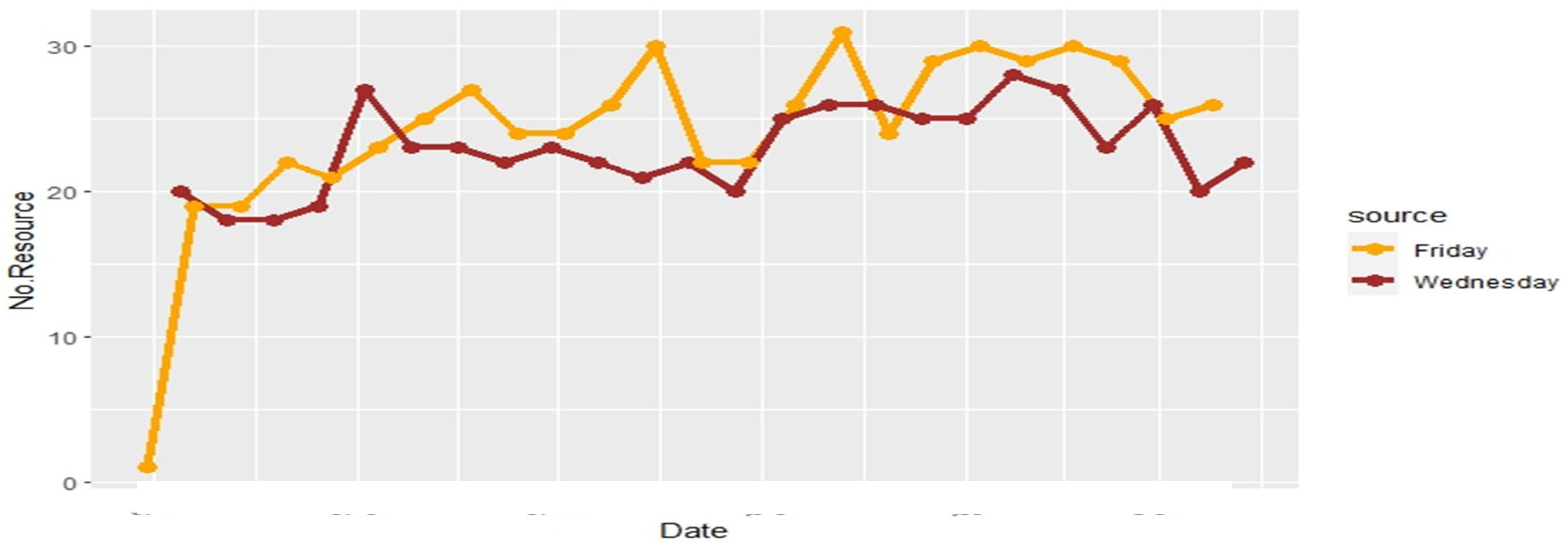
Additionally, Figure 3 shows the number of resources present each day. It indicates that out of 68 resources, a maximum of 10 resources are present on any given day. This implies that not all resources are present throughout the event log period. Further, it is seen that not all resources are present throughout the event log period. The column ‘Nan’ pertains to activities without specified resources. To determine which working days have the highest workload and the number of cases reviewed, Figure 5 and Figure 6 indicate that the green line represents the workload on Sunday, which is the lowest, followed by Saturday in red, with the least amount of work. This is due to fewer resources being present on these days. Conversely, Figure 7 shows that Monday and Tuesday have the highest workload as more resources are present on these days. This data shows a predictable trend of resource presence and the amount of work done. Notably, the resource coded 112 is active most days, including holidays.
Figure 3.
Frequency of resources with a specific number of working days
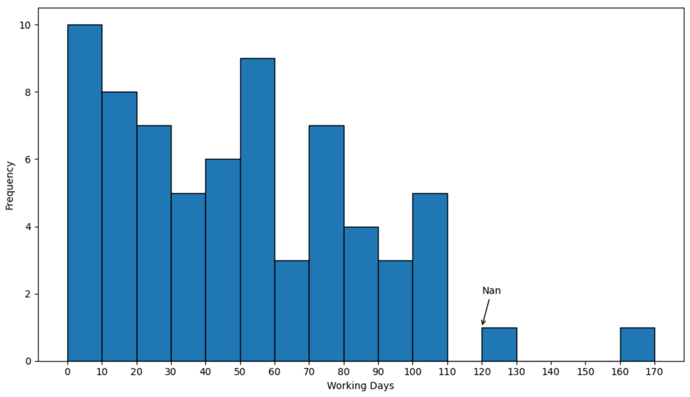
Figure 4.
Total working day per resource
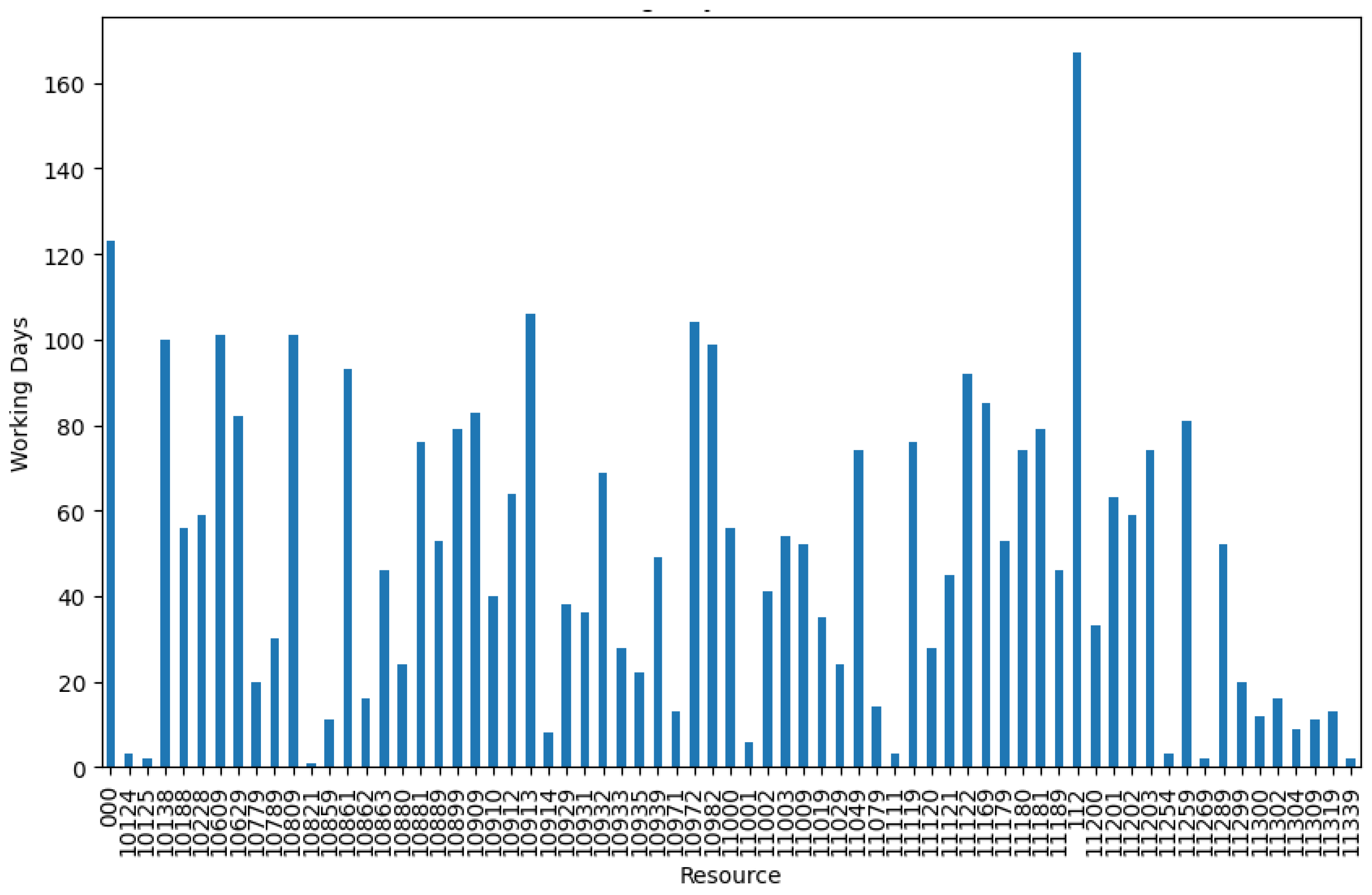
Figure 5.
Chart of the workload of the week and the most active resources.
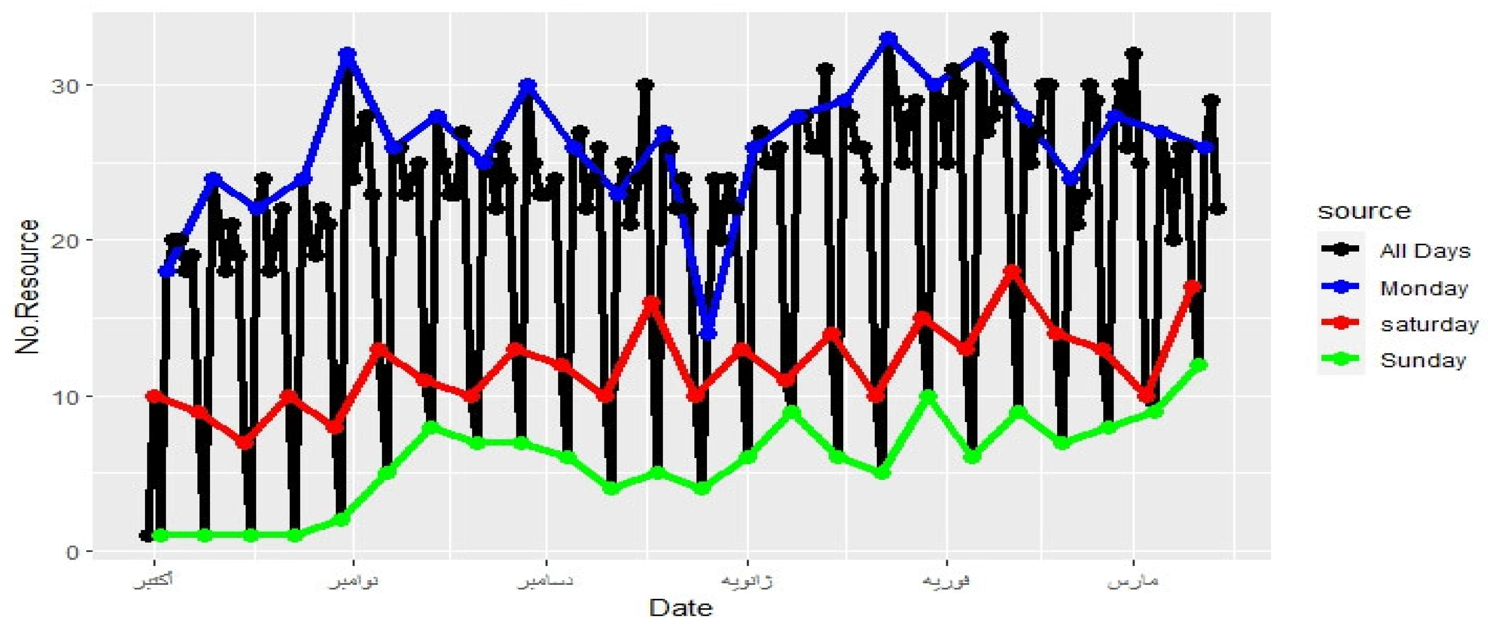
Figure 6.
The number of active resources in two working days of the week.
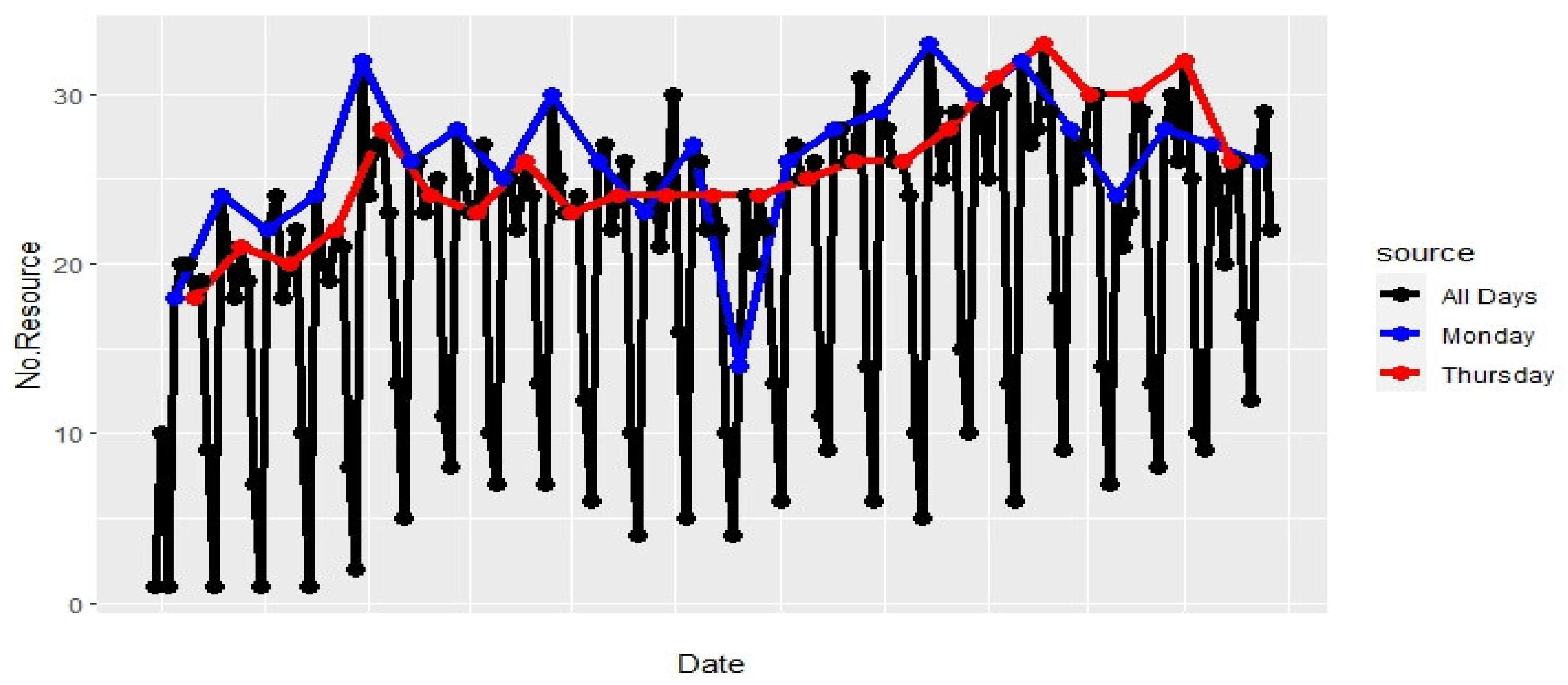
Figure 7.
The number of active bans in the rest of the week.
We can determine each resource’s working hours throughout the day to gauge their efficiency at the workplace. Table 7 indicates the total period from the first to the last presence for each resource during the event log period. This information can also be observed in resource 112.
Based on working hours and presence time, 112 is a machine, unlike other human resources. In the next step, we analyze the impact of activities by their type over time for each case.
According to the process report, some resources do not initiate activities, meaning they lack the ‘complete’ lifecycle attribute in the main data. For example, resource 112 only approves and dispatches tasks. Some resources started working from a specific point in the event log, such as 11289. Some resources, such as 11169, have a high workload and perform more tasks. This insight helps identify the bottleneck stage where a resource is involved.
Next, we examine the relationship between the resource handling the request and the outcome. Table 8 gives the frequency of cases classified based on their final evaluation by the resource. We only considered resources that participated in evaluating at least one request. It can be observed that resources can only adopt three approaches: reject, approve, or cancel against loan/overdraft requests. Table 8 shows that resource 112, an automated resource, plays a role in approving three practical requests.
Table 9 pertains to all resources that have conducted all three evaluations on the requests. Upon identifying resource 112, we investigate the three requests approved by this automated resource, namely cases 177083, 180310, and 198310. Additionally, upon review, all three cases belong to separate process paths.
Resource 112, being automated, has a very high working time. Following it, other resources have the highest working time in the report, which will be analyzed further to determine their efficiency and productivity.
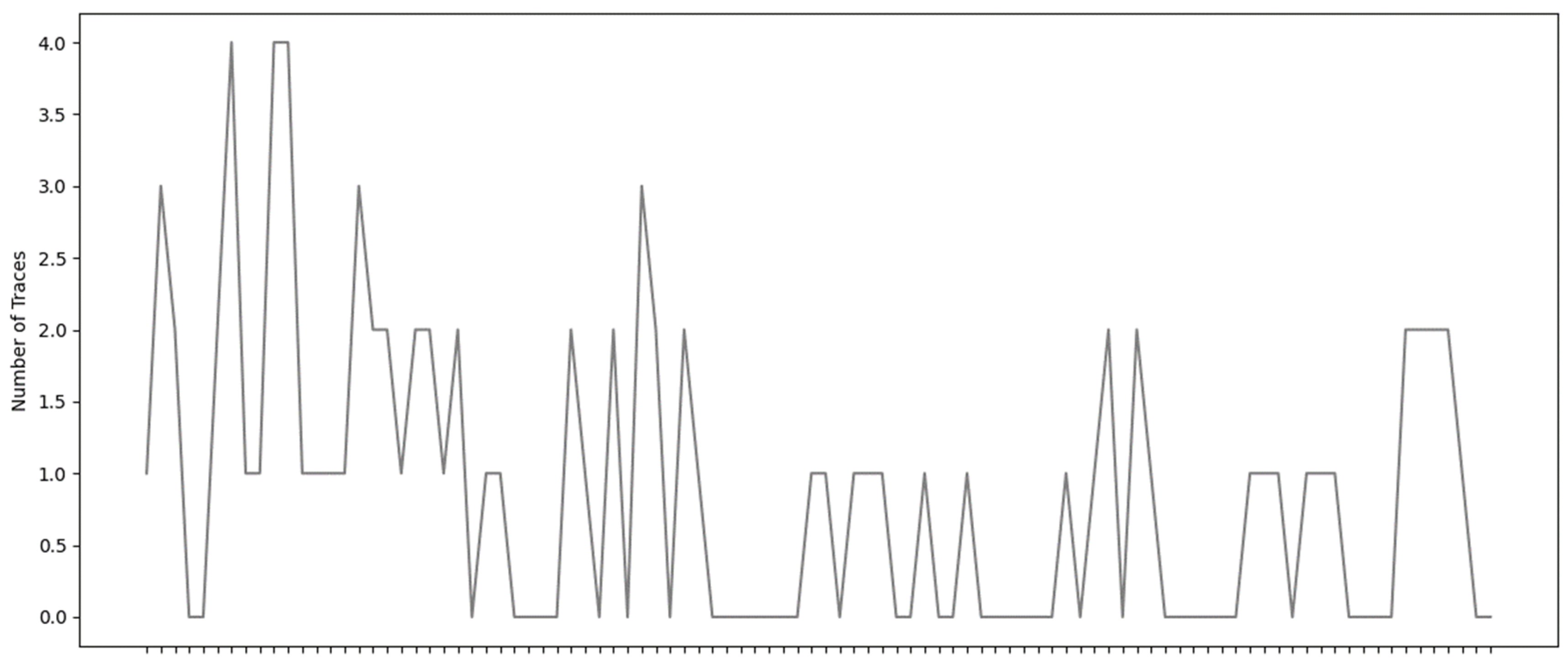
Figure 8 illustrates the number of cases reviewed by resource 11169 in one day. This chart, defined based on time intervals, monitors working days minute by minute and counts the cases for a specified resource. In Figure 8, resource 11169 shows a peak working period from 8:55 to 9:10, with about 7 cases under review. Also, from 11:30 to 12:30, the lunch break is estimated to have zero workload. After the break, a more stable workload peak is observed. Generally, the morning hours from 8:00 to 11:30 have double the peak workload compared to the rest of the day. According to Figure 10, most cases are related to one or two paths under this resource’s review.
Table 7 shows that resource 10972 is one of the busiest resources. According to Figure 10, this resource usually reviews one case but has low efficiency, according to Table 13. Furthermore, it can be seen that the behavior of resources can differ depending on their activities. Figure 9 and Figure 17 show the distribution of work done by resources over two randomly selected days. These Figures demonstrate the overall behavior of resources and the amount of work they perform.
Figure 9.
Workload of all resources on 2012/30/01.
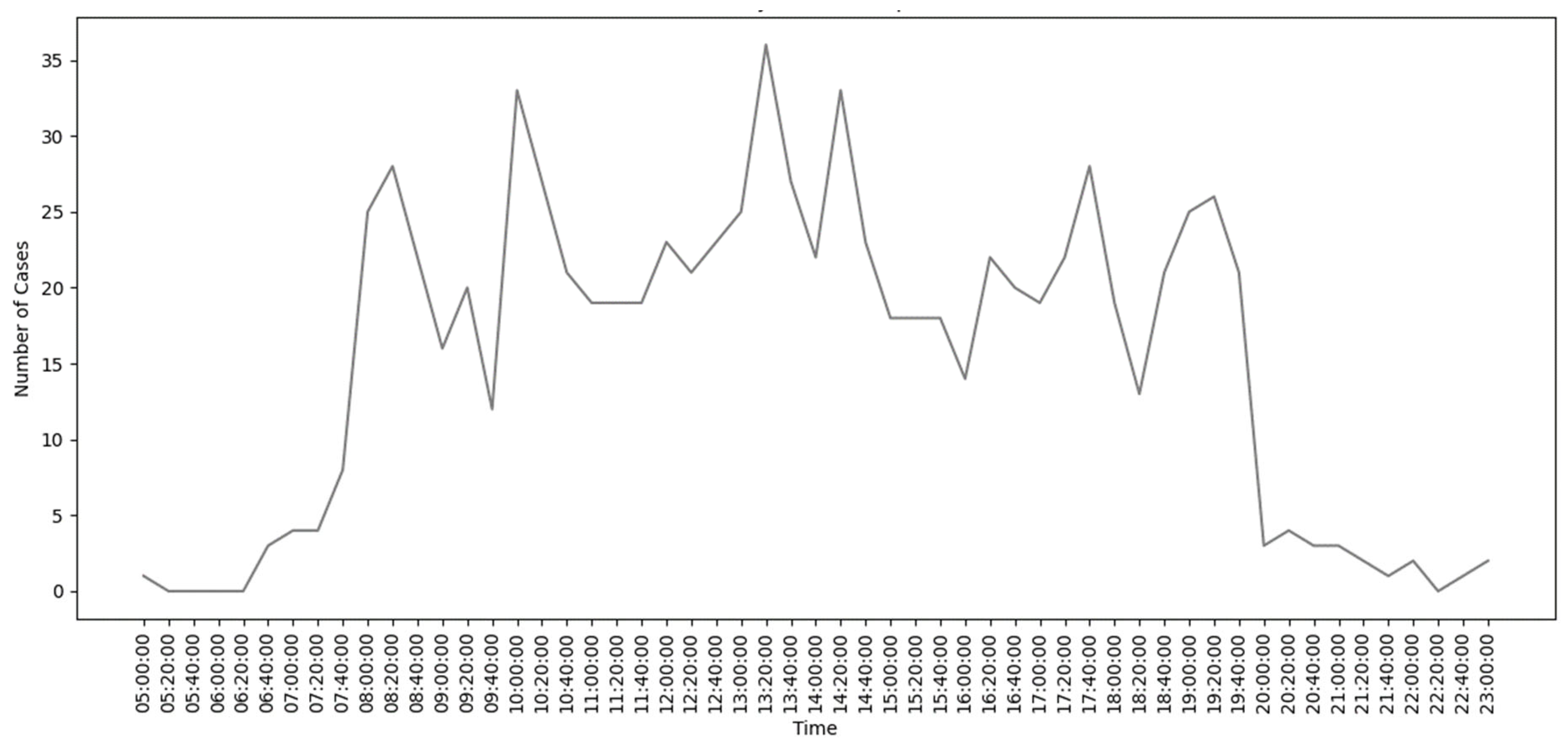
Figure 10.
The number of cases reviewed by the source is 10972 on 2012/09/03.
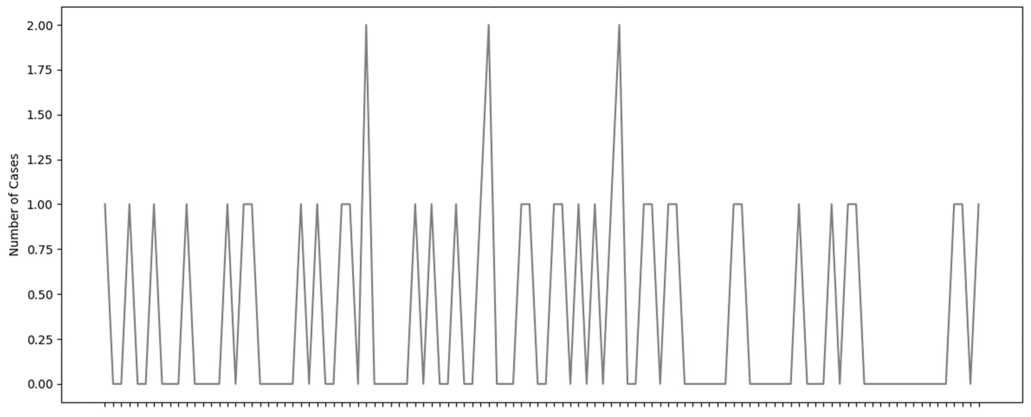
Figure 11.
Number of unique variants under review by source 11169 on 2012/01/31.
One of the points mentioned in (Maruster & Van der Aalst, 2013) is concurrent work. This study examined the fact that resources might perform several tasks simultaneously over time. It was eventually shown that performing concurrent tasks prolongs the activities. This study calculates concurrent work, as shown in Figure 12. The concurrent work index for each resource indicates the number of tasks a resource handles simultaneously within a time interval. In essence, the current activity being performed can overlap with another activity in four possible states, and based on these states, the time spent on concurrent work is obtained. This method is used to assess the performance of working resources and for data envelopment analysis.
4.4. Process Discovery
In this section, we aim to discover the activity diagrams within the event log using three algorithms: Alpha, Inductive, and Heuristic. Once discovered, these diagrams can be transformed into more interpretable charts. Each process discovery algorithm offers varying levels of accuracy, generalizability, and interpretability. Initially, we observe that the start activity for all cases is ‘A_SUBMITTED,’ the end activities and their frequencies are presented in Table 10. Ultimately, it is inferred that the primary process path has 3429 repetitions, accounting for only 26% of the remaining paths.
After employing various miners, the goal is to select the best miner. Table 11 addresses some of these criteria. An algorithm performs better if it fits well and has good generalizability. Additionally, the simplicity of the model enhances its interpretability. Based on these criteria, the Heuristic Miner algorithm demonstrates superior performance. The output of this algorithm is shown in Figure 13.
Our analysis focused on uncovering activity diagrams from an event log using three process discovery algorithms: Alpha, Inductive, and Heuristic. Each algorithm provided different precision, generalization, and interpretability levels, crucial for practical process analysis and optimization.
The initial observation Table 10 revealed that the activity ‘A_SUBMITTED’ is the consistent starting point for all cases, which indicates a well-defined initiation step in the process. Table 9 lists the end activities and their frequencies, showing that ‘A_DECLINED’ is the most frequent outcome, occurring 3429 times. This high frequency of declined cases suggests a significant area where the process may fail to meet its goals. Other notable end activities include ‘W_Valideren aanvraag’ and ‘W_Completeren aanvraag,’ indicating stages where the process either validates or completes requests.
Table 11 compares the performance of the Alpha, Inductive, and Heuristic Miners based on simplicity, generalization, precision, and average fitness. Given these performance metrics, the Heuristic Miner is the best choice due to its superior precision and fitness despite its complexity. The resulting process model from the Heuristic Miner, illustrated in Figure 13, accurately captures the intricacies of the event log activities. The comparison highlights the importance of selecting the proper process discovery algorithm. The Heuristic Miner, with its higher precision and fitness, is more suited for detailed process analysis. Managers should prioritize precision and fitness in their choice of tools to ensure that the insights derived are accurate and actionable.
While the simplicity of the Alpha Miner makes it appealing for quick overviews, the detailed accuracy provided by the Heuristic Miner is essential for in-depth analysis. Managers should strive for a balance between model simplicity and the need for detailed insights. This balance will help make the models interpretable and valuable for strategic decision-making. The application of the Heuristic Miner algorithm and the subsequent detailed analysis provide critical insights into process efficiency and areas for improvement. By leveraging these insights, managers can enhance process performance, reduce inefficiencies, and ensure a robust and continuous improvement framework.
4.5. Proposed RDEA Implication
To evaluate the efficiency of resources in the event log, we first define metrics for measuring efficiency. These metrics are extracted from the event log. Some of these metrics are desirable to minimize because they indicate low efficiency. Conversely, there are metrics that we aim to maximize. Metrics that should be minimized are considered inputs, while metrics that should be maximized are considered outputs.
Table 12.
Input and output sets.
| Inputs | Outputs |
| total idle time | average work time |
| = average idle time | total work time |
| = duration of simultaneous work | = amount of loan processed |
| the number of scheduled tasks | = average time present in the event log |
| = number of completed case | |
| = number of reviewed cases | |
| = number of cases with the same start and end resources |
We use Data Envelopment Analysis (DEA) to evaluate resource efficiency. This study employs scenario-based robust DEA (RDEA) to evaluate the units. The data must be normalized using equation (12) in directional radial models (Han et al., 2011). This process brings the obtained data for each metric into the range of [0, 1].
We consider the = 0.009 and = 0.04 results in each scenario as follows:
1. The key performance indicators (KPIs) obtained are estimated to be up to ten percent less than their actual values.
2. The KPIs are accurately obtained.
3. The KPIs are estimated to be ten to twenty percent more than their actual values.
The probability of occurrence for each scenario is considered 35%, 40%, and 25%, respectively.
Table 13.
Efficiency scores of resources.
| DMU | Scenarios | Rank | ||
| W1 | W2 | W3 | ||
| 112 | 1.0 | 1.0 | 1.0 | 1 |
| 10124 | 0.097 | 0.122 | 0.138 | 49 |
| 10125 | 0.432 | 0.487 | 0.468 | 6 |
| 10138 | 0.156 | 0.168 | 0.18 | 32 |
| 10188 | 0.055 | 0.075 | 0.085 | 65 |
| 10228 | 0.093 | 0.146 | 0.154 | 42 |
| 10609 | 0.25 | 0.221 | 0.241 | 19 |
| 10629 | 0.098 | 0.121 | 0.126 | 50 |
| 10779 | 0.077 | 0.086 | 0.088 | 62 |
| 10789 | 0.157 | 0.153 | 0.158 | 36 |
| 10809 | 0.084 | 0.12 | 0.136 | 52 |
| 10859 | 0.215 | 0.329 | 0.314 | 16 |
| 10861 | 0.106 | 0.134 | 0.142 | 44 |
| 10862 | 0.111 | 0.126 | 0.128 | 47 |
| 10863 | 0.09 | 0.09 | 0.096 | 61 |
| 10880 | 0.194 | 0.235 | 0.25 | 21 |
| 10881 | 0.091 | 0.118 | 0.113 | 55 |
| 10889 | 0.086 | 0.11 | 0.114 | 56 |
| 10899 | 0.209 | 0.199 | 0.193 | 23 |
| 10909 | 0.119 | 0.15 | 0.152 | 41 |
| 10910 | 0.197 | 0.28 | 0.287 | 18 |
| 10912 | 0.141 | 0.171 | 0.176 | 33 |
| 10913 | 0.127 | 0.121 | 0.121 | 45 |
| 10914 | 0.112 | 0.112 | 0.117 | 51 |
| 10929 | 0.273 | 0.273 | 0.293 | 17 |
| 10931 | 0.108 | 0.163 | 0.172 | 39 |
| 10932 | 0.108 | 0.126 | 0.131 | 48 |
| 10933 | 0.084 | 0.076 | 0.083 | 63 |
| 10935 | 0.142 | 0.181 | 0.179 | 31 |
| 10939 | 0.081 | 0.1 | 0.1 | 60 |
| 10971 | 0.269 | 0.301 | 0.306 | 15 |
| 10972 | 0.207 | 0.246 | 0.253 | 20 |
| 10982 | 0.151 | 0.162 | 0.164 | 35 |
| 11000 | 0.094 | 0.114 | 0.129 | 53 |
| 11001 | 0.168 | 0.187 | 0.173 | 28 |
| 11002 | 0.089 | 0.098 | 0.095 | 59 |
| 11003 | 0.15 | 0.202 | 0.199 | 26 |
| 11009 | 0.1 | 0.114 | 0.11 | 54 |
| 11019 | 0.061 | 0.08 | 0.082 | 64 |
| 11029 | 0.324 | 0.408 | 0.384 | 9 |
| 11049 | 0.094 | 0.101 | 0.098 | 58 |
| 11079 | 0.115 | 0.179 | 0.194 | 34 |
| 11111 | 0.476 | 0.656 | 0.612 | 4 |
| 11119 | 0.092 | 0.106 | 0.107 | 57 |
| 11120 | 0.352 | 0.306 | 0.307 | 13 |
| 11121 | 0.125 | 0.169 | 0.167 | 37 |
| 11122 | 0.178 | 0.189 | 0.192 | 25 |
| 11169 | 0.125 | 0.134 | 0.126 | 43 |
| 11179 | 0.149 | 0.177 | 0.18 | 30 |
| 11180 | 0.144 | 0.19 | 0.187 | 29 |
| 11181 | 0.159 | 0.187 | 0.196 | 27 |
| 11189 | 1.0 | 1.0 | 1.0 | 1 |
| 11200 | 0.145 | 0.133 | 0.15 | 40 |
| 11201 | 0.144 | 0.159 | 0.151 | 38 |
| 11202 | 0.11 | 0.126 | 0.134 | 46 |
| 11203 | 0.171 | 0.197 | 0.211 | 24 |
| 11254 | 0.001 | 0.001 | 0.001 | 67 |
| 11259 | 0.226 | 0.217 | 0.222 | 22 |
| 11269 | 1.0 | 1.0 | 1.0 | 1 |
| 11289 | 0.329 | 0.316 | 0.321 | 14 |
| 11299 | 0.408 | 0.389 | 0.402 | 8 |
| 11300 | 0.391 | 0.468 | 0.495 | 7 |
| 11302 | 0.569 | 0.445 | 0.463 | 5 |
| 11304 | 0.28 | 0.364 | 0.385 | 12 |
| 11309 | 0.32 | 0.397 | 0.373 | 11 |
| 11319 | 0.28 | 0.396 | 0.434 | 10 |
| 11339 | 0.033 | 0.038 | 0.036 | 66 |
The efficiency scores of various DMUs across the three scenarios are listed in the table, along with their corresponding ranks. Top performers, such as DMUs 112, 11189, and 11269, consistently score 1.0 across all scenarios, indicating robust efficiency under varied conditions and earning them the first rank. Mid-range performers, including DMUs like 10125 and 11029, display moderate efficiency scores ranging between 0.4 and 0.5, suggesting stable yet suboptimal performance. In contrast, low performers such as DMUs 11254 and 11339 have significantly lower efficiency scores, consistently ranking at the bottom and highlighting areas needing substantial improvement. DMUs 112, 11189, and 11269 exemplify excellent performance and resilience across all scenarios. Managers should analyze these units’ operational practices to identify best practices that can be replicated across other units. These could include workflow optimizations, effective resource management, or innovative problem-solving techniques. Units such as 10124 and 10863, which show significant variability and lower efficiency scores, require targeted interventions. Managers should investigate the root causes of inefficiencies, such as process bottlenecks, resource underutilization, or external factors affecting performance. Addressing these issues can help improve their overall efficiency and stability.
Figure 14.
Comparison of Certain model and RDEA.
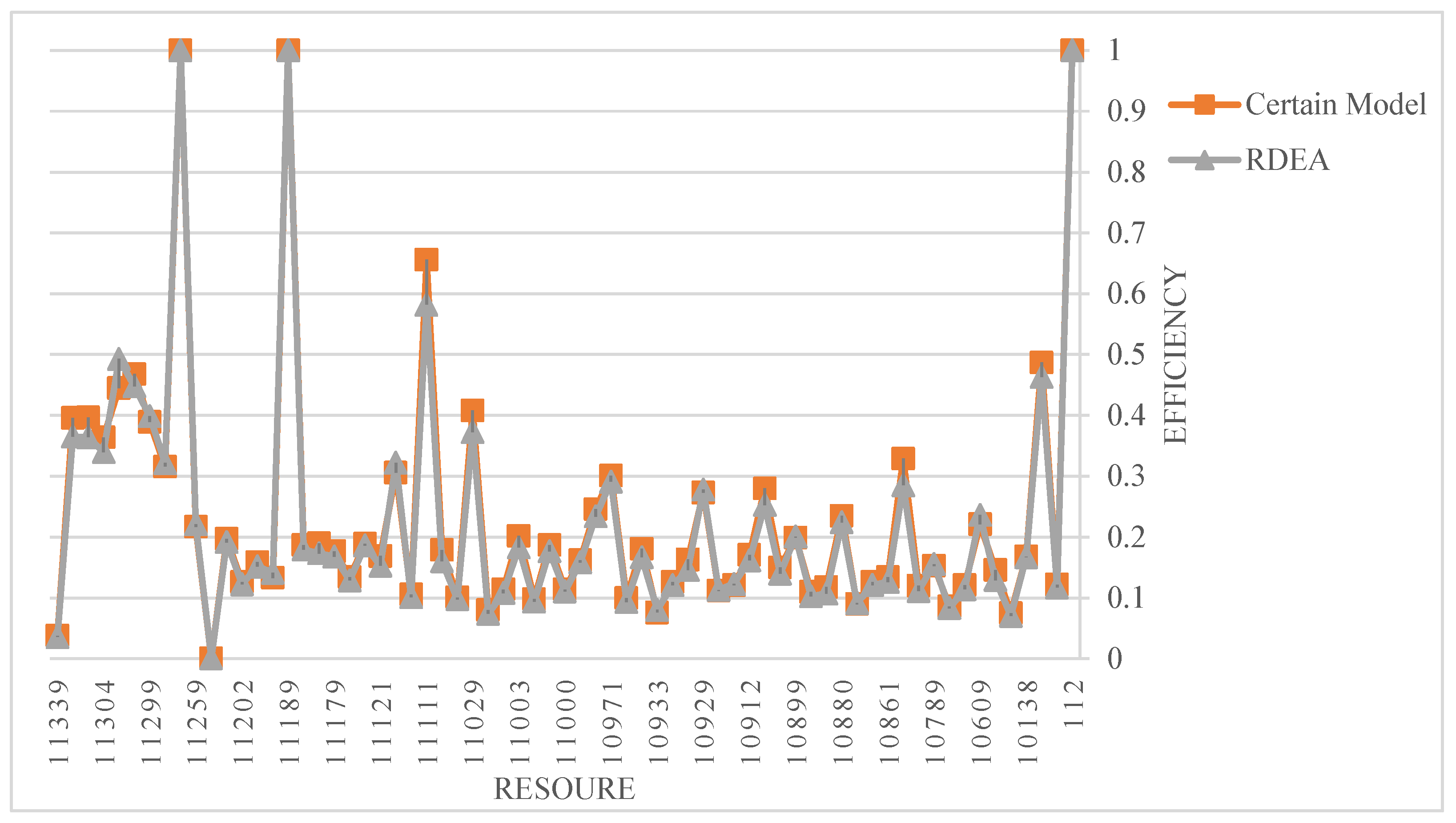
The variation in efficiency scores across different scenarios underscores the importance of scenario-based planning. Managers should develop contingency plans to mitigate the impact of KPI fluctuations, ensuring sustained performance under varying conditions. This approach can help prepare for unexpected changes and maintain operational efficiency. The efficiency scores provide valuable insights for resource allocation. High-performing units could be leveraged to mentor and support lower-performing ones. Additionally, redistributing resources might be necessary to optimize overall efficiency. Ensuring that resources are used where they are most effective can enhance overall organizational performance. Establishing benchmarks based on top-performing units and setting achievable targets for other DMUs is crucial. Implementing continuous improvement programs focusing on areas highlighted by the DEA analysis can enhance overall efficiency. Regularly updating these benchmarks and improvement programs ensures that the organization remains competitive and efficient. Understanding the robustness of efficiency scores under different scenarios aids in making informed decisions. Managers can prioritize interventions in units that show significant efficiency declines in worse-case scenarios, ensuring a balanced approach to performance management. This robust approach ensures that improvements are sustainable and aligned with organizational goals, even under varying external conditions.
4.6. Prediction of Loan Status
The dataset comprises various attributes (CaseID, Throughput, WorkingResources, Amount, Activities, Rework, Earliest Starting Resource, Final Resource, and Avg_Wait, and Loan Status). As previously mentioned, a loan’s final status can be one of four states: approved, declined, canceled, or undecided. We assign numerical values 0, 1, and 2 to the remaining states by excluding the records related to undecided cases. Additionally, two columns indicating the source of initiation and termination are appended to the table as categorical data (used exclusively for the ANN model).
After implementing the appropriate models, the output is as follows:
Table 14.
Obtained table of features with the target value.
| Case ID | Throughput | W.R | Amount | Activities | Rework | ES.R | Final Resource | Avg_Wait | L.S |
| 173694 | 1.000000e+00 | 10 | 7000 | 59 | 30.0 | 10609.0 | 10912.0 | 14.287189 | 2 |
| 179591 | 6.664793e-01 | 16 | 20000 | 92 | 70.0 | 10861.0 | 112.0 | 105.390192 | 2 |
| 188485 | 6.392675e-01 | 14 | 7000 | 84 | 53.0 | 10861.0 | 112.0 | 15.379321 | 2 |
| 189805 | 6.258252e-01 | 18 | 25000 | 92 | 55.0 | 10609.0 | 10629.0 | 22.020927 | 2 |
| 183405 | 6.141806e-01 | 23 | 200000 | 141 | 118.0 | 10138.0 | 10889.0 | 20.202247 | 2 |
After implementing the appropriate models, the output is as follows:
Table 15.
Performance of supervised ML models.
| Model | Accuracy | Precision | Recall | F1 Score |
| ANN | 85% | 83% | 84% | 83% |
| KNN | 82% | 77% | 78% | 77% |
| GB | 91% | 91% | 91% | 91% |
The GB (Gradient Boosting) model outperforms the other models in predicting loan approval or rejection and is therefore used for more detailed analysis. The performance metrics for each class are as follows:
GB model shows exceptional performance with a 94% F1 Score and a precision of 99%. This high precision is crucial for minimizing the approval of risky loans, thereby reducing the bank’s exposure to bad debt. With an F1 Score and recall of 90%, the model effectively identifies applications that should be declined, ensuring that high-risk applicants are not mistakenly approved. Similar performance is observed for canceled loans, with the model maintaining an F1 Score and recall of 90%. This indicates robust handling of applications either withdrawn by applicants or canceled by the bank due to incomplete information or other reasons.
4.7. Prediction of the Next Activity
After assigning letters to each activity, Table 16 contains the name of each case and the process path it has followed. Based on this path, the LSTM neural network predicts the next activity.
Table 16.
Performance of supervised ML models divided by each class.
| Class | Accuracy | Precision | Recall | F1 Score |
| Accept | 89% | 99% | 94% | 94% |
| Declined | 94% | 86% | 90% | 90% |
| Canceled | 91% | 89% | 90% | 90% |
Table 17.
Variant of each case.
| Case id | Variant |
| 173688 | abcssdkelmtstttttnutugfohu |
| 173691 | abcssssdeklmtstttkplmtttttnutuuuuuofghu |
| 173694 | abcssssssssdeklmtstkplmttttttttttkplmtttttttttt... |
| 173697 | abj |
| 173700 | abj |
| 214364 | abcssssdeklmtstkpImtttttttnut |
| 214367 | abj |
| 214370 | abrrjr |
| 214373 | abrrcsrsdkelmtstt |
| 214376 | abrrjr |
The final model has a loss of 0.4 on the test data and an accuracy of approximately 87%. Its confusion matrix is presented in Figure 15:
4.8. Behavior Analysis
4.8.1. Behavior of Resources Involved in the Loan Process
The x-axis represents time measured in weeks, so customers are observed over 25 weeks. The gap between the red line (resources with tasks more than once) and the black line (total tasks performed) indicates that most resources perform tasks more than once over time.
Figure 16.
Number of works by resources in 25 weeks.
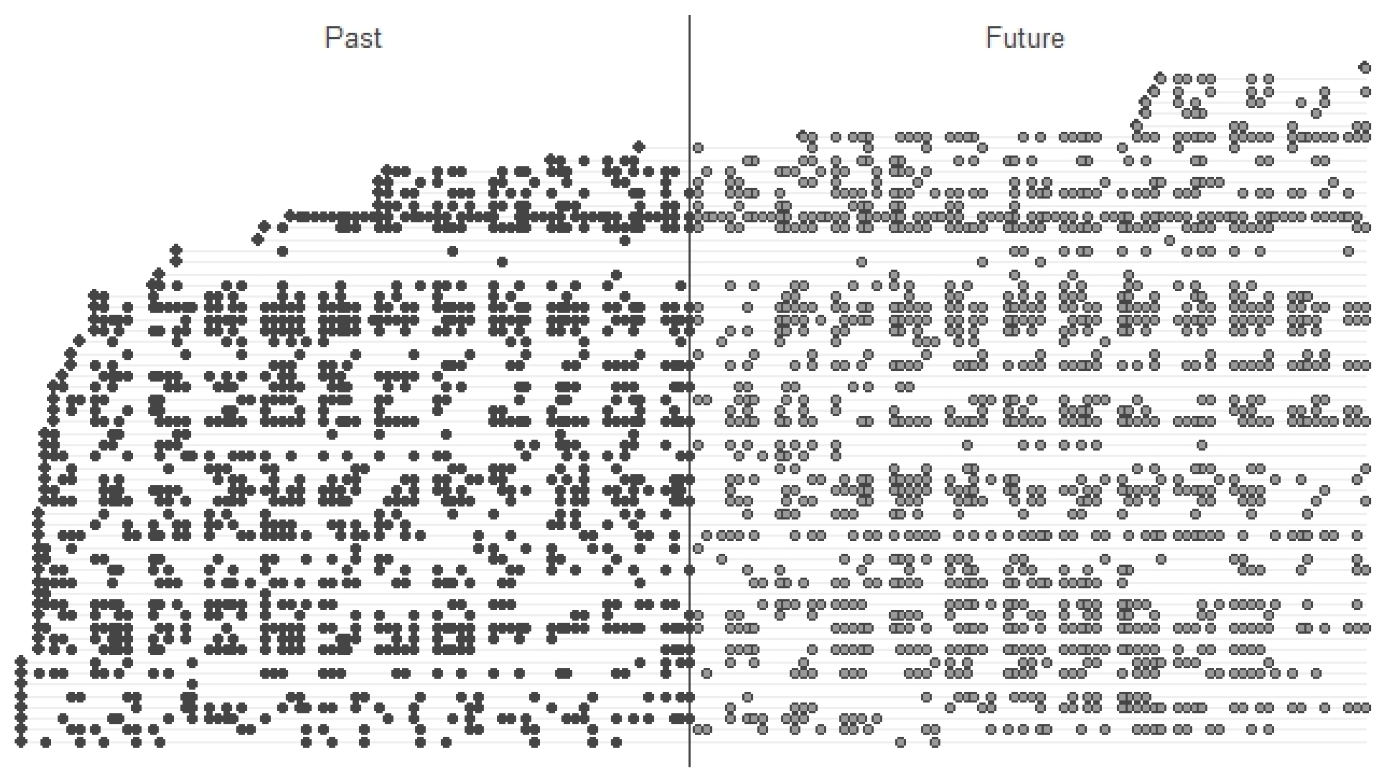
4.8.2. Activity of Resources Over the Time Horizon
Figure 18 shows the start time of the resources’ tasks. The horizontal axis represents time, and the vertical axis represents resources. The points indicate the start time of the tasks for each customer. According to the Figure, if the timeline’s middle is considered the dividing point, the likelihood of model mismatch in the data is low.
Figure 17.
Start work time of resources.
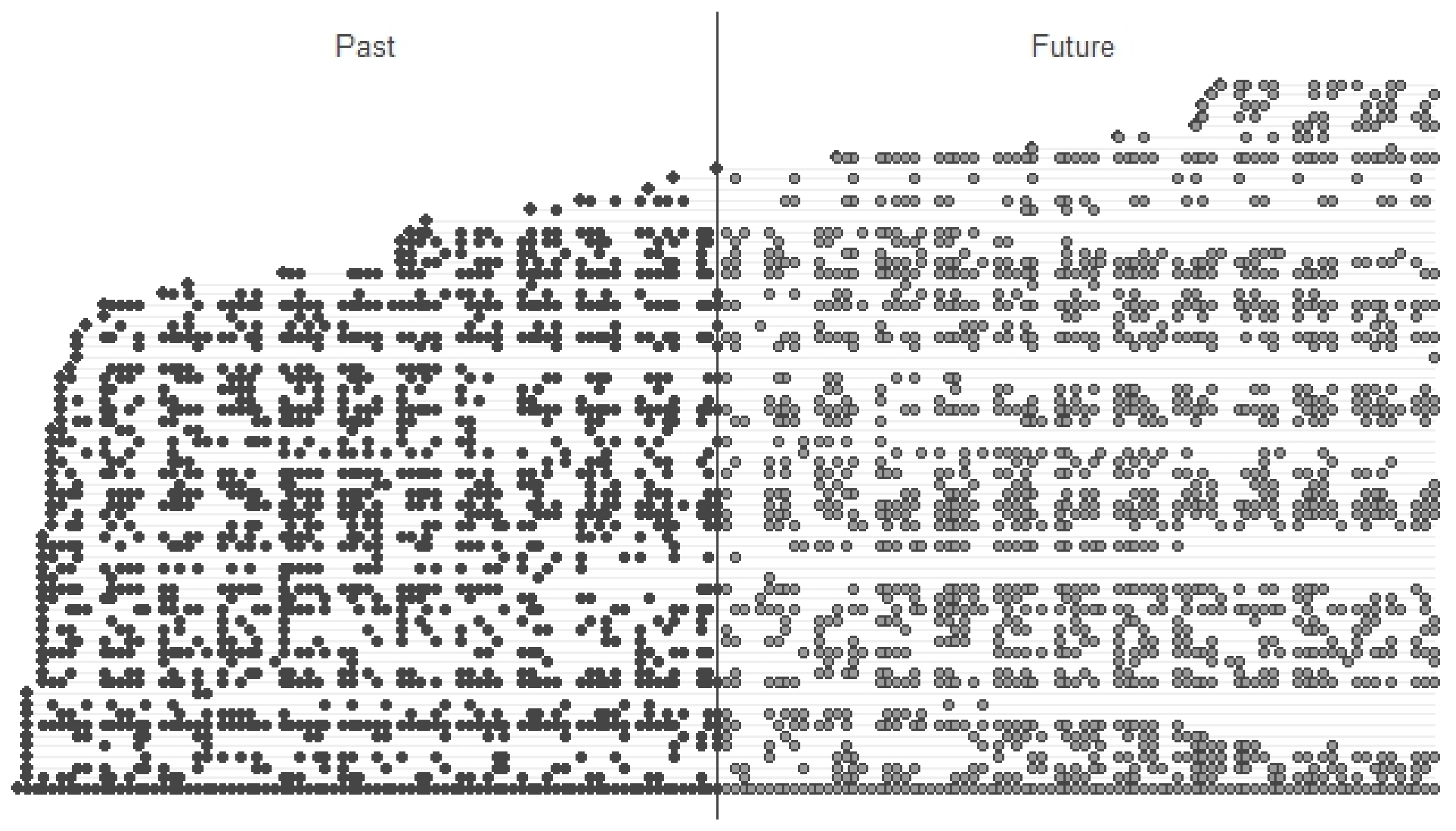
Figure 18.
Group A working resources per time.
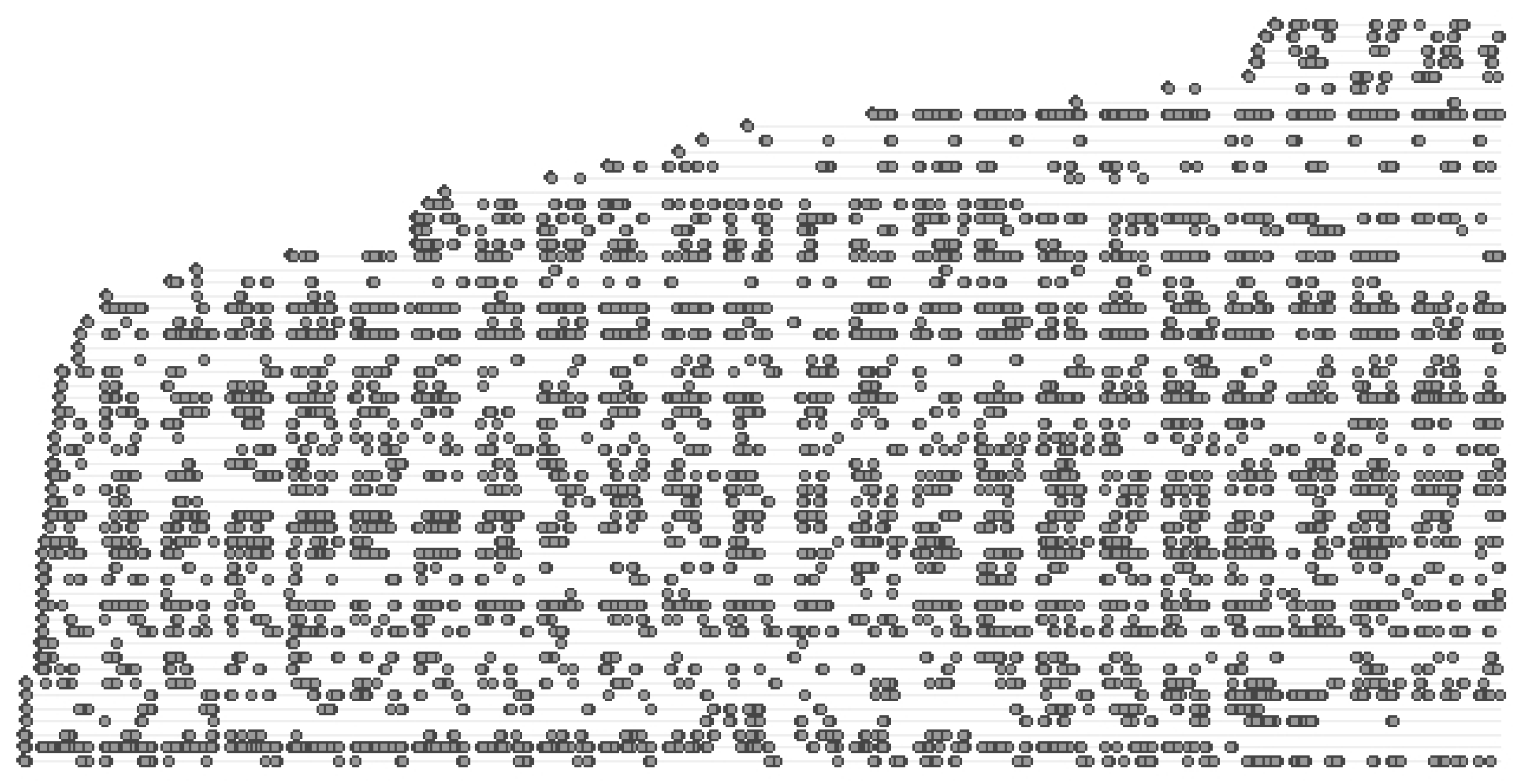
Now, the data is divided into three parts based on the type of activity the resources perform. The types of activities include 1-O, 2-W, and 3-A. The scatter plot for each type is shown in Figure 18 when the data is filtered.
Figure 19.
Group O working resources per time.
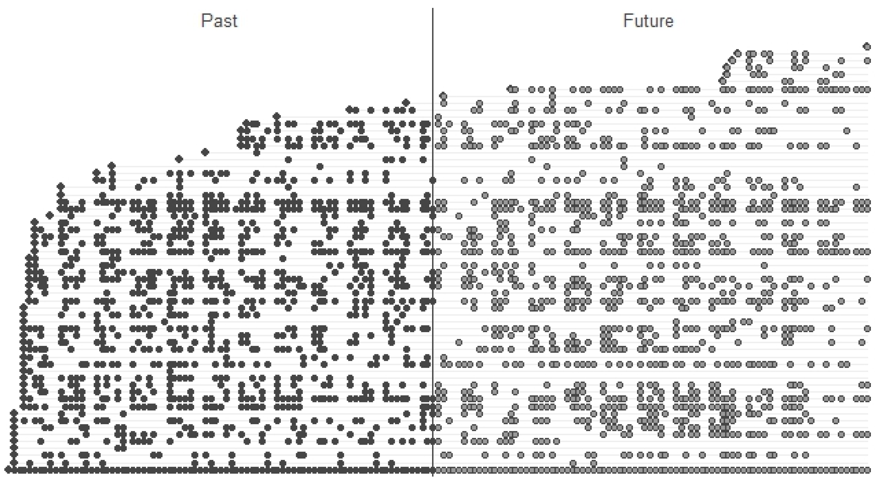
Figure 20.
Group W working resources per time.
4.8.3. Prediction of Resource Behavior
The prediction analysis aims to address the following three points:
- What is the likelihood of each type of activity being performed by the resource in the future?
- How many activities are expected to be performed in the future?
- How much time will be spent on activities in the future? (This is only done for group W activities.)
4.8.3.1. Model Evaluation
We use the BG/NBD, BG/CNBD-k, MBG/CNBD-k, and Pareto/NBD models for prediction. The model assumptions are as follows:
- While the resource is active, the activities performed by the resource in the period t follow a Poisson distribution with a mean of λt.
- The variation in the activity rate among resources follows a gamma distribution with shape r and scale α.
- Each resource becomes inactive after each activity with probability p.
- The variation in p follows a beta distribution with shape parameters a and b.
K is the Erlang distribution parameter. For k=1, the exponential distribution represents the time interval between the resources’ activities. Table 18 shows the best model for our estimation.
Table 18.
Estimated parameter and model accuracy.
| Model | Group | k | r | α | a | b | Log-likelihood | Measurement Error |
| BG/NBD | O | 1 | 2.210217 | 7.35683 | 16.72848 | 9991.288 | -2311.05 | 2.59% |
| A | 1 | 2.151856 | 7.570773 | 2.00E-05 | 2298.765 | -2242.51 | 10.17% | |
| W | 1 | 2.101796 | 6.779813 | 6.62E-05 | 703.1266 | -2166.4 | 4.47% | |
| BG/CNBD-k | O | 2 | 2.082449 | 3.414529 | 27.25052 | 9996.939 | -2190.8 | 2.25% |
| A | 2 | 2.117672 | 3.649783 | 1.88E+01 | 9990.269 | -2117.17 | 16.91% | |
| W | 2 | 1.940769 | 3.109838 | 3.26E-05 | 781.9663 | -2028.28 | 4.47% | |
| MBG/NBD | O | 1 | 2.205368 | 7.338904 | 15.70053 | 9993.16 | -2311.13 | 5.96% |
| A | 1 | 2.151582 | 7.569427 | 2.46E-05 | 1566.838 | -2242.51 | 16.91% | |
| W | 1 | 2.103013 | 6.782676 | 2.26E-06 | 664.6548 | -2166.4 | 4.55% | |
| MBG/CNBD-k | O | 2 | 2.075718 | 3.403359 | 25.45929 | 10000 | -2190.93 | 6.22% |
| A | 2 | 2.136701 | 3.678407 | 1.84E+01 | 10000 | -2117.19 | 16.91% | |
| W | 2 | 1.940785 | 3.110092 | 4.30E-06 | 61.46382 | -2028.28 | 4.55% | |
| Pareto/NBD | O | 1 | 2.147124 | 6.959706 | 0.013459 | 11.27909 | -2312.25 | 9.50% |
| A | 1 | 2.15245 | 7.570375 | 3.43E-06 | 455.8619 | -2242.51 | 16.91% | |
| W | 1 | 2.101516 | 6.780728 | 2.36E-06 | 628.723 | -2166.4 | 4.55% |
Table 18.
Best performing models for each group.
| Activity | Selected Model | Error Percentage | |
| O | BG/CNBD-k | 2.59 | |
| A | BG/NBD | 10.17 | |
| W | MBG/NBD | 4.55 |
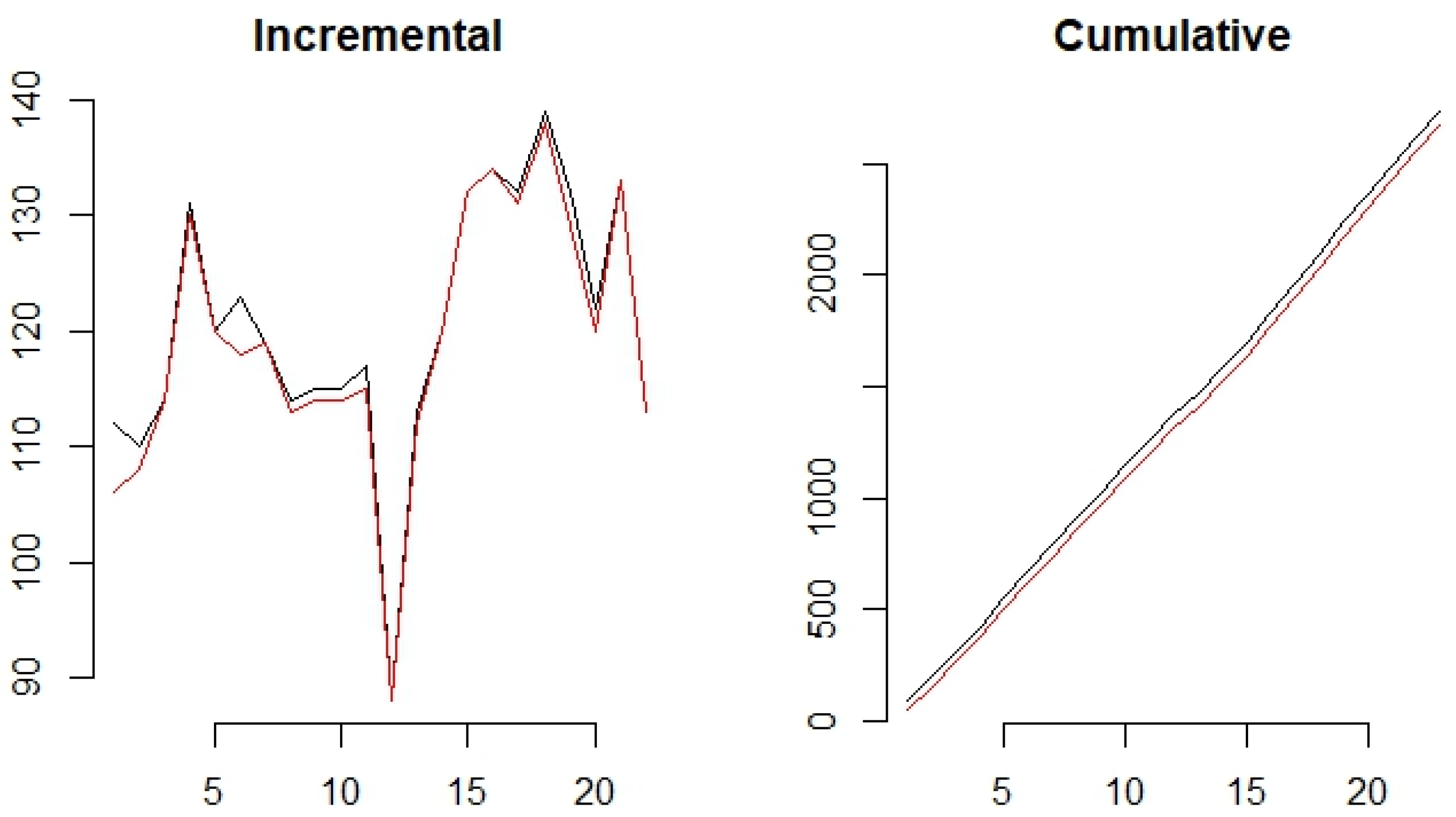
Figure 21.
Accuracy of model for group A (black line is actual data).
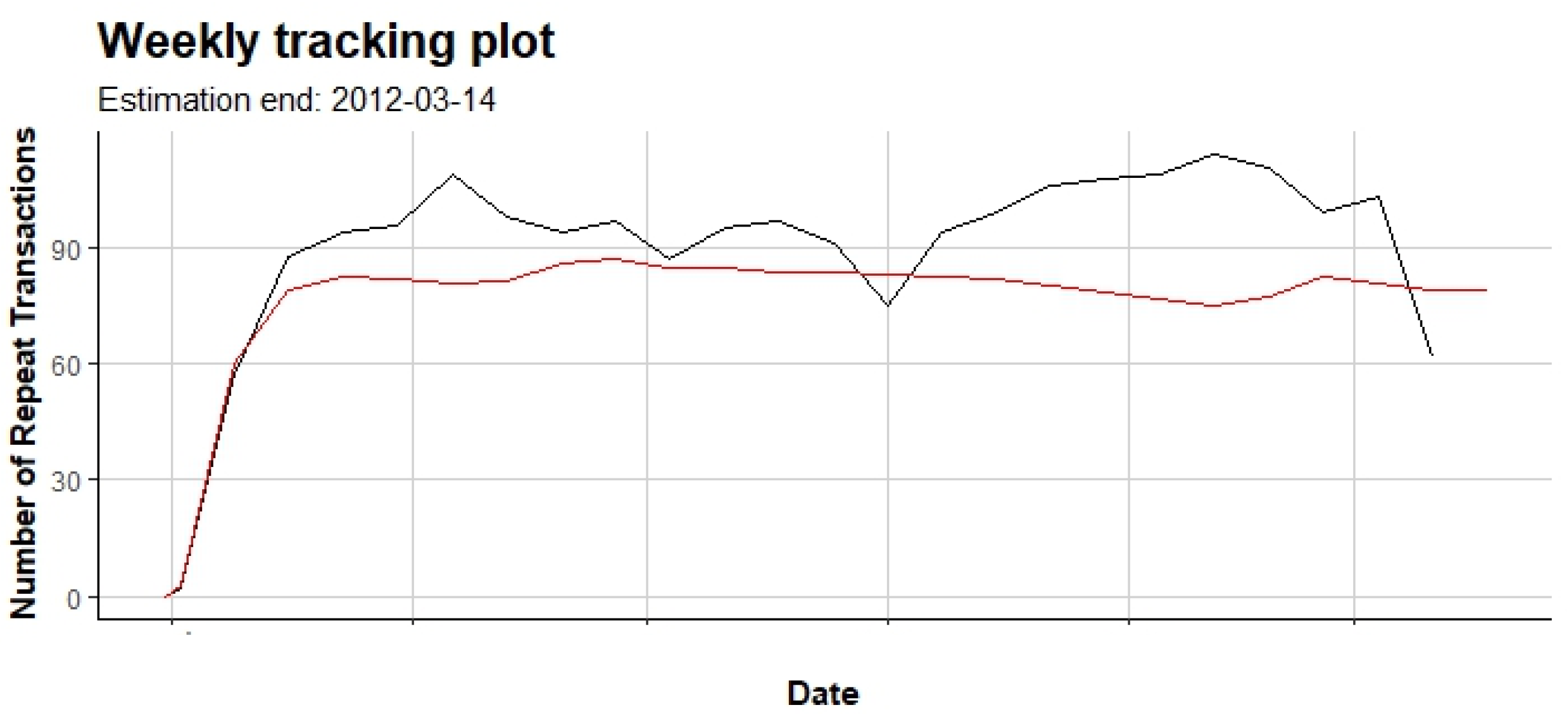
Figure 22.
Accuracy of model for group O (black line is actual data).
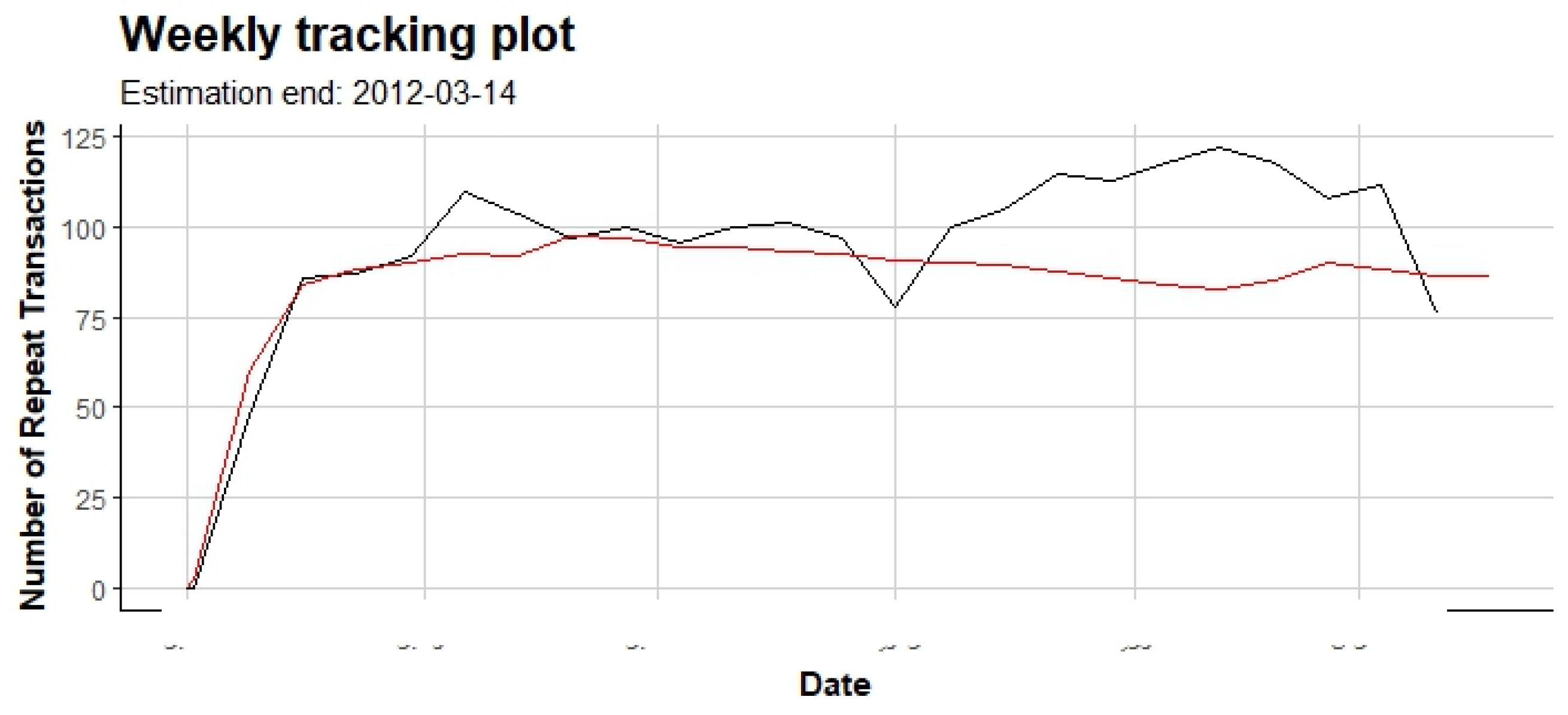
Figure 23.
Accuracy of model for group W (black line is actual data).
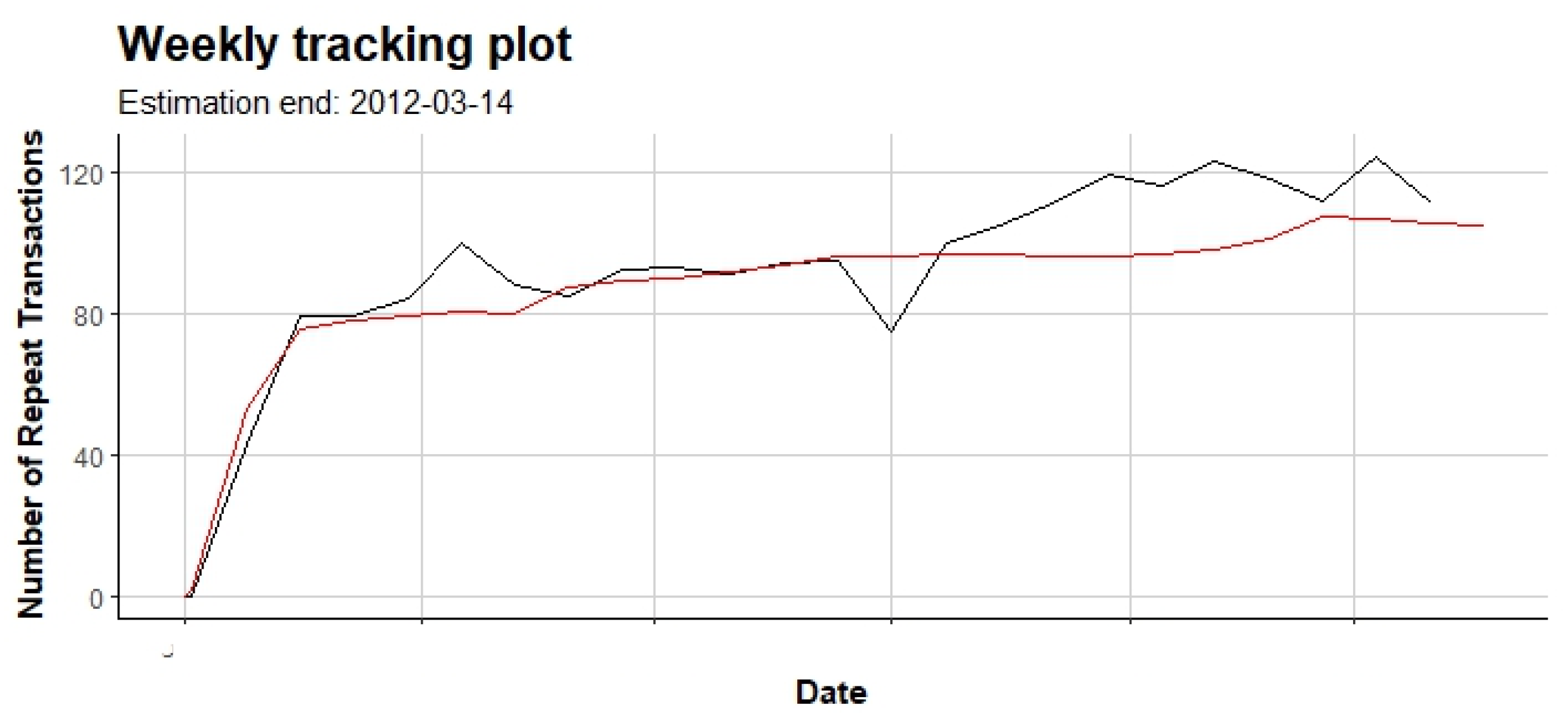
Figure 24 shows the time spent and the statistical model constructed from it. This model helps determine the amount of time each resource will spend performing activities in the future.
5. Conclusions
One of the goals of process mining is to measure the efficiency of the tasks performed. This study attempted to measure resource efficiency using the DEA method. Thus, DEA methods can be used along with process mining tools to evaluate resource efficiency in organizations better. DEA and process mining provide complementary approaches for understanding efficiency. DEA helps compare the relative efficiency of decision-making units, identify best practices, and provide recommendations for improvement. On the other hand, process mining focuses on understanding the actual process flow, analyzing performance metrics, identifying root causes of inefficiencies, and enabling continuous monitoring for ongoing process improvement. The integration of prediction and behavior analysis further extends the capabilities of process mining and DEA, enabling organizations to anticipate future trends and behaviors and proactively address inefficiencies. Organizations can optimize operations, mitigate risks, and drive continuous improvement by leveraging predictive analytics and behavior analysis techniques. Process mining and DEA represent indispensable tools for organizations seeking to enhance operational efficiency, drive continuous improvement, and maintain competitiveness in today’s dynamic business landscape. By embracing these disciplines and leveraging their analytical capabilities, organizations can gain actionable insights, optimize processes, and achieve strategic objectives.
In future research, root cause analysis can be utilized in process mining. The root causes of inefficiencies identified by DEA can be determined by analyzing event logs and process models. By identifying deviations from the expected process flow or behavioral patterns that contribute to inefficiencies, organizations can target specific improvements to address these root causes directly. This analysis can include identifying bottlenecks and their relationship with the efficiency obtained from the DEA method.
| 1 | Data Envelopment Analysis |
References
- Abe, M. Counting Your Customers One by One: A Hierarchical Bayes Extension to the Pareto/NBD Model. Marketing Science 2009, 28(3), 541–553. [Google Scholar] [CrossRef]
- Adriansyah, A.; van Dongen, B. F.; van der Aalst, W. M. P.; Andrews, R. Process Discovery Using Event Logs: A Literature Survey. ACM Computing Surveys (CSUR) 2011, 44(1), 1–62. [Google Scholar]
- Altman, N. S. An introduction to kernel and nearest-neighbor nonparametric regression. The American Statistician 1992, 46(3), 175–185. [Google Scholar] [CrossRef]
- Batislam, E.; Denizel, M.; Filiztekin, A. Empirical validation and comparison of models for customer base analysis. International Journal of Research in Marketing 2007, 24(3), 201–209. [Google Scholar] [CrossRef]
- Bautista, A. D.; Wangikar, L.; Akbar, S. M. K. Process mining-driven optimization of a consumer loan approvals process; BPI Challenge, 2012. [Google Scholar]
- Ben-Tal, A.; Nemirovski, A. Robust optimization: methodology and applications. Mathematical programming 2009, 107(1-2), 1–41. [Google Scholar] [CrossRef]
- Bertsimas, D.; Sim, M. Robust optimization: formulation, implementation, and applications. In Handbook of data-based decision making in education; Springer; Boston, MA, 2004; pp. 431–454. [Google Scholar]
- Bose, R. J. C.; van der Aalst, W. M. Process mining applied to the BPI challenge 2012: Divide and conquer while discerning resources. Business Process Management Workshops: BPM 2012 International Workshops, Tallinn, Estonia; 2013. [Google Scholar]
- Buijs, J. C.; Reijers, H. A.; van Dongen, B. F. Resolving deviant behavior in process models; 2014. [Google Scholar]
- Carmona, J.; van Dongen, B. F.; Solti, A.; Weidlich, M. Automated Discovery of Process Models from Event Logs: Review and Benchmark. ACM Transactions on Management Information Systems (TMIS) 2018, 9(1), 1–57. [Google Scholar]
- Charnes, A.; Cooper, W. W.; Rhodes, E. Measuring the efficiency of decision-making units. European journal of operational research 1978, 2(6), 429–444. [Google Scholar] [CrossRef]
- Charnes, A.; Cooper, W. W.; Golany, B.; Seiford, L.; Stutz, J. Foundations of data envelopment analysis for Pareto-Koopmans efficient empirical production functions. Journal of Econometrics 1985, 30(1-2), 91–107. [Google Scholar] [CrossRef]
- Charnes, A.; Cooper, W. W.; Seiford, L.; Stutz, J. Invariant multiplicative efficiency and piecewise Cobb-Douglas envelopments. Operations Research Letters 1983, 2(3), 101–103. [Google Scholar] [CrossRef]
- Chen, T.; Guestrin, C. XGBoost: A Scalable Tree Boosting System. In Proceedings of the 22nd ACM SIGKDD International Conference on Knowledge Discovery and Data Mining; ACM, 2016; pp. 785–794. [Google Scholar] [CrossRef]
- Cooper, W. W.; Seiford, L. M.; Tone, K. Data envelopment analysis: a comprehensive text with models, applications, references and DEA-solver software; Springer, 2007; Vol. 2. [Google Scholar]
- Cover, T. M.; Hart, P. E. Nearest neighbor pattern classification. IEEE Transactions on Information Theory 1967, 13(1), 21–27. [Google Scholar] [CrossRef]
- Dumas, M.; La Rosa, M.; Mendling, J.; Reijers, H. A. Fundamentals of Business Process Management; Springer, 2018. [Google Scholar]
- Ehrenberg, A. S. C. The pattern of consumer purchases. Applied Statistics 1959, 8(1), 26–41. [Google Scholar] [CrossRef]
- Fix, E.; Hodges, J. L. Discriminatory Analysis. Nonparametric Discrimination: Consistency Properties. Report Number 4, Project Number 21-49-004; USAF School of Aviation Medicine; Randolph Field, Texas, 1951.
- Friedman, J. H. Greedy function approximation: A gradient boosting machine. Annals of Statistics 2001, 29(5), 1189–1232. [Google Scholar] [CrossRef]
- Graves, A.; Mohamed, A.; Hinton, G. Speech recognition with deep recurrent neural networks. 2013 IEEE International Conference on Acoustics, Speech and Signal Processing; IEEE, 2013; pp. 6645–6649. [Google Scholar] [CrossRef]
- Hammer, M. What is Business Process Management? In Handbook on Business Process Management 1; Springer, 2010; pp. 3–16. [Google Scholar]
- Han, J.; Pei, J.; Kamber, M. Data Mining: Concepts and Techniques; Elsevier, 2011. [Google Scholar]
- Harmon, P. Business Process Change: A Business Process Management Guide for Managers and Process Professionals; Morgan Kaufmann, 2014. [Google Scholar]
- Hochreiter, S.; Schmidhuber, J. Long Short-Term Memory. Neural Computation 1997, 9(8), 1735–1780. [Google Scholar] [CrossRef]
- Hoppe, D.; Wagner, M. Customer base analysis using stochastic modeling: An application to a large retailer. OR Spectrum 2007, 29(3), 421–433. [Google Scholar]
- LeCun, Y.; Bengio, Y.; Hinton, G. Deep Learning. Nature 2015, 521(7553), 436–444. [Google Scholar] [CrossRef]
- Leemans, S. J. J.; Fahland, D.; van der Aalst, W. M. P.; van Dongen, B. F. Efficiently Mining Generalized Association Rules. IEEE Transactions on Knowledge and Data Engineering 2013, 25(2), 303–318. [Google Scholar]
- Leung, S. C.; Tsang, S. O.; Ng, W.-L.; Wu, Y. A robust optimization model for multi-site production planning problem in an uncertain environment. European journal of operational research 2007, 181(1), 224–238. [Google Scholar] [CrossRef]
- Lu, X.; Zhang, L.; Lee, S. C. A tree-based approach for analyzing collaborative business processes, 2014.
- Ma, S.; Liu, J. S. Hierarchical Bayes models for “buy till you die” data. Journal of Business & Economic Statistics 2007, 25(4), 536–545. [Google Scholar]
- Maruster, L.; van der Aalst, W. M. P. Real-life event log selection: Method and case study; 2013. [Google Scholar]
- Mulvey, J. M.; Vanderbei, R. J.; Zenios, S. A. Robust optimization of large-scale systems. Operations research 1995, 43(2), 264–281. [Google Scholar] [CrossRef]
- Platzer, M.; Reutterer, T. Incorporating regularity in transaction timings into customer base analysis. Journal of Retailing and Consumer Services 2016, 30, 67–77. [Google Scholar]
- Reutterer, T.; Platzer, M.; Schröder, T. Extending Pareto/NBD for customer base analysis using continuous and discrete covariates. Journal of the Academy of Marketing Science 2020, 48(1), 157–175. [Google Scholar]
- Rumelhart, D. E.; Hinton, G. E.; Williams, R. J. Learning representations by back-propagating errors. Nature 1986, 323(6088), 533–536. [Google Scholar] [CrossRef]
- Sutskever, I.; Vinyals, O.; Le, Q. V. Sequence to sequence learning with neural networks. In Advances in Neural Information Processing Systems; 2014; pp. 3104–3112. [Google Scholar]
- Tax, N.; Verenich, I.; La Rosa, M.; Dumas, M. Predictive business process monitoring with LSTM neural networks. In International Conference on Advanced Information Systems Engineering; Springer, Cham, 2017; pp. 477–492. [Google Scholar]
- Teinemaa, I.; Dumas, M.; La Rosa, M. Mining Declarative Process Models from Event Logs Containing Noise. BPM Workshops; 2012; pp. 153–164. [Google Scholar]
- Thanassoulis, E. Introduction to the Theory and Application of Data Envelopment Analysis: A Foundation Text with Integrated Software; Springer, 2001. [Google Scholar]
- Van Dongen, B. F.; de Medeiros, A. K. A.; Verbeek, H. M. W.; Weijters, A. J. M. M.; van der Aalst, W. M. P. The ProM Framework: A New Era in Process Mining Tool Support. In Applications and Theory of Petri Nets; 2005; pp. 34–39. [Google Scholar]
- Van der Aalst, W. M. P.; Reijers, H. A.; Song, M. Discovering Social Networks from Event Logs. Computer Supported Cooperative Work (CSCW) 2005, 14(6), 549–593. [Google Scholar] [CrossRef]
- Van der Aalst, W. M. P. Process Mining: Discovery, Conformance and Enhancement of Business Processes; Springer, 2011. [Google Scholar]
- Van der Aalst, W. M. P.; Weijters, A. J. M. M.; Maruster, L. Workflow Mining: Discovering Process Models from Event Logs. IEEE Transactions on Knowledge and Data Engineering 2004, 16(9), 1128–1142. [Google Scholar] [CrossRef]
- Van der Aalst, W. M. P.; Weijters, A. J. M. M.; Maruster, L. The Business Process Intelligence Challenge 2012: Discovering Bottlenecks and Deviations in Processes; Springer, 2012. [Google Scholar]
- Van Der Aalst, W.; van der Aalst, W. Data science in action; Springer, 2016. [Google Scholar]
Figure 1.
Categorize event log requests.

Figure 2.
Working time distribution chart based on hours of the day.
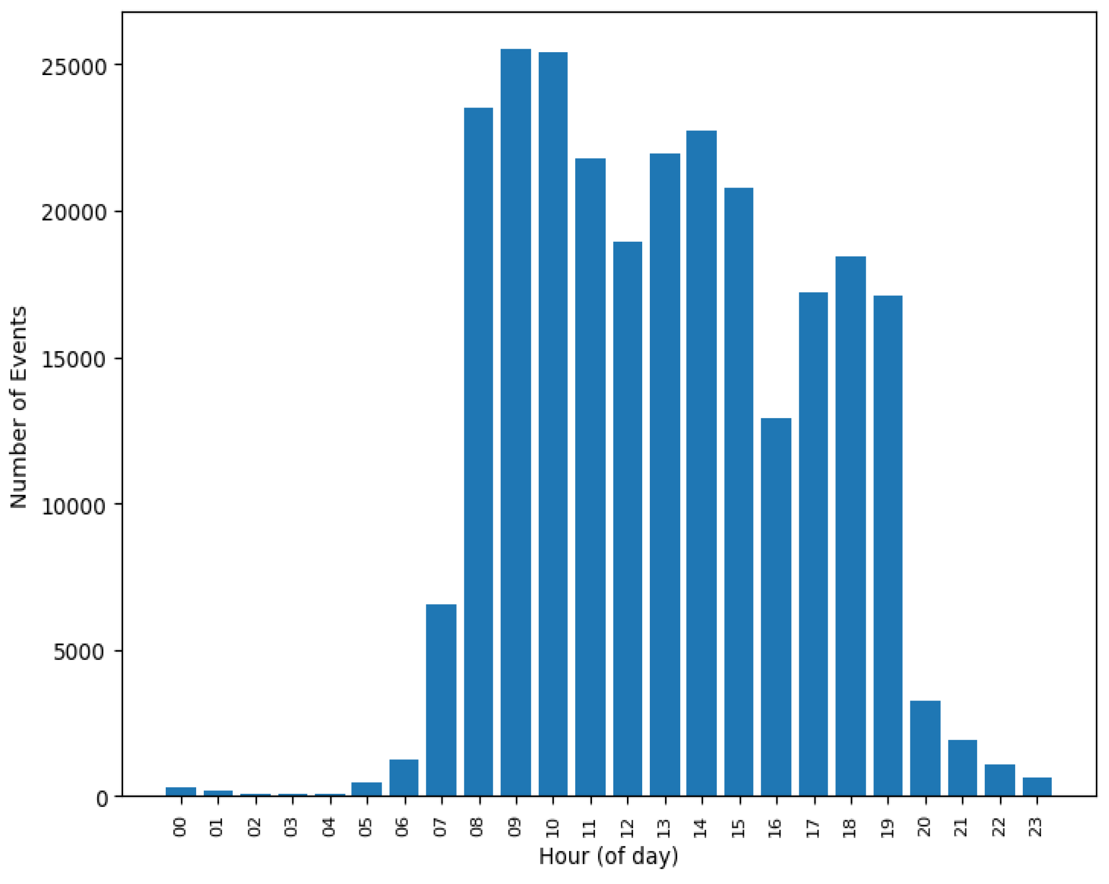
Figure 8.
The number of cases reviewed by resource 11169.
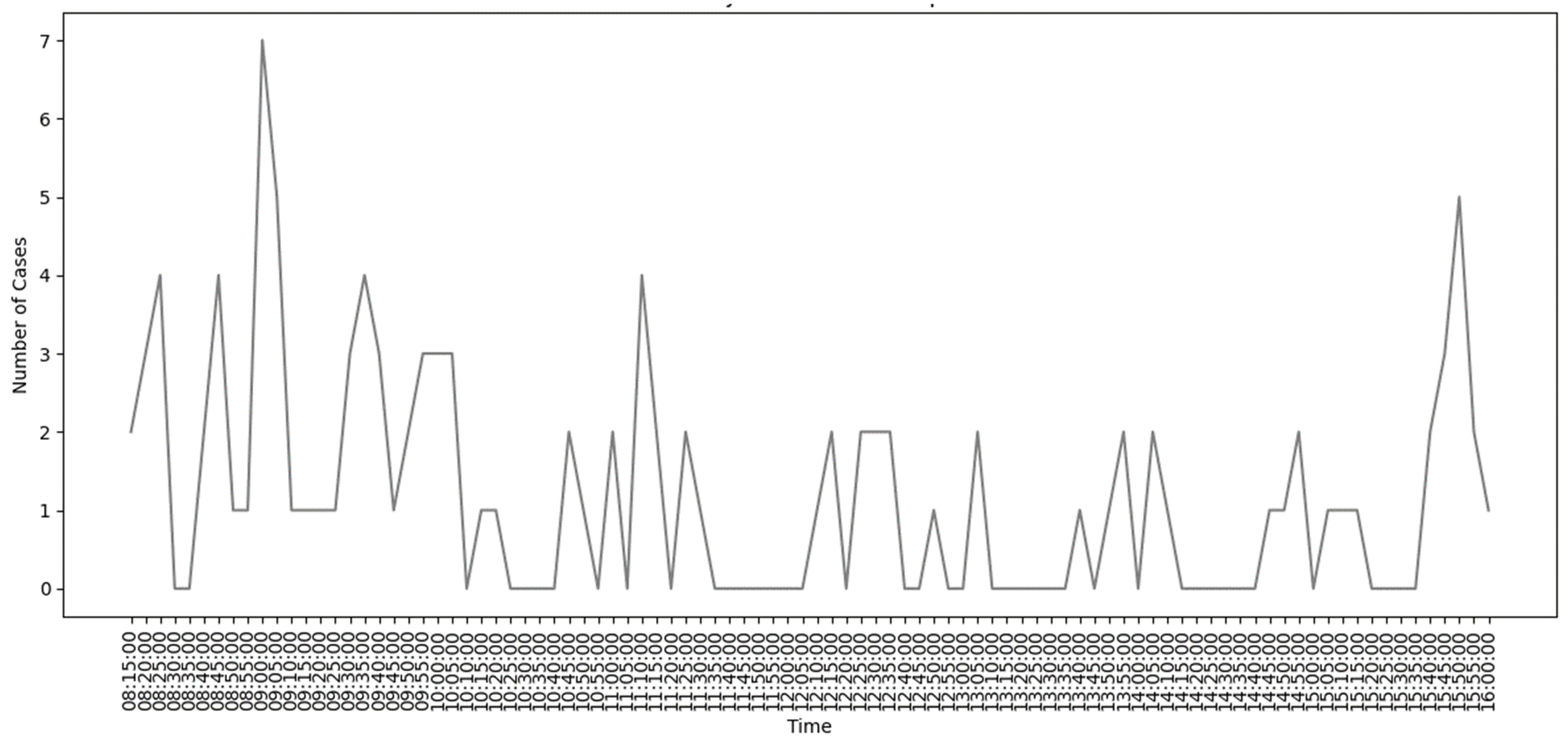
Figure 12.
Four classes of simultaneous working.
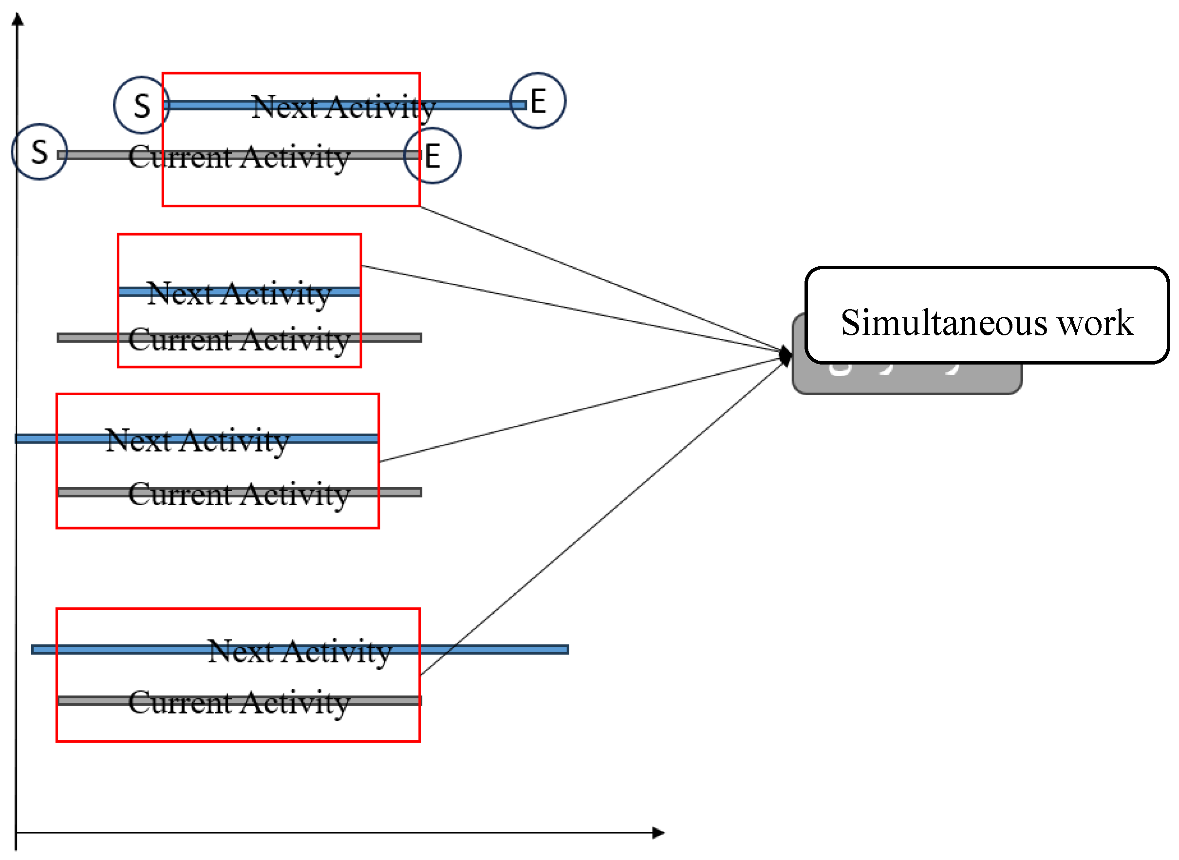
Figure 13.
Process model based on HM algorithm.

Figure 15.
Predicted vs. actual activity matrix.
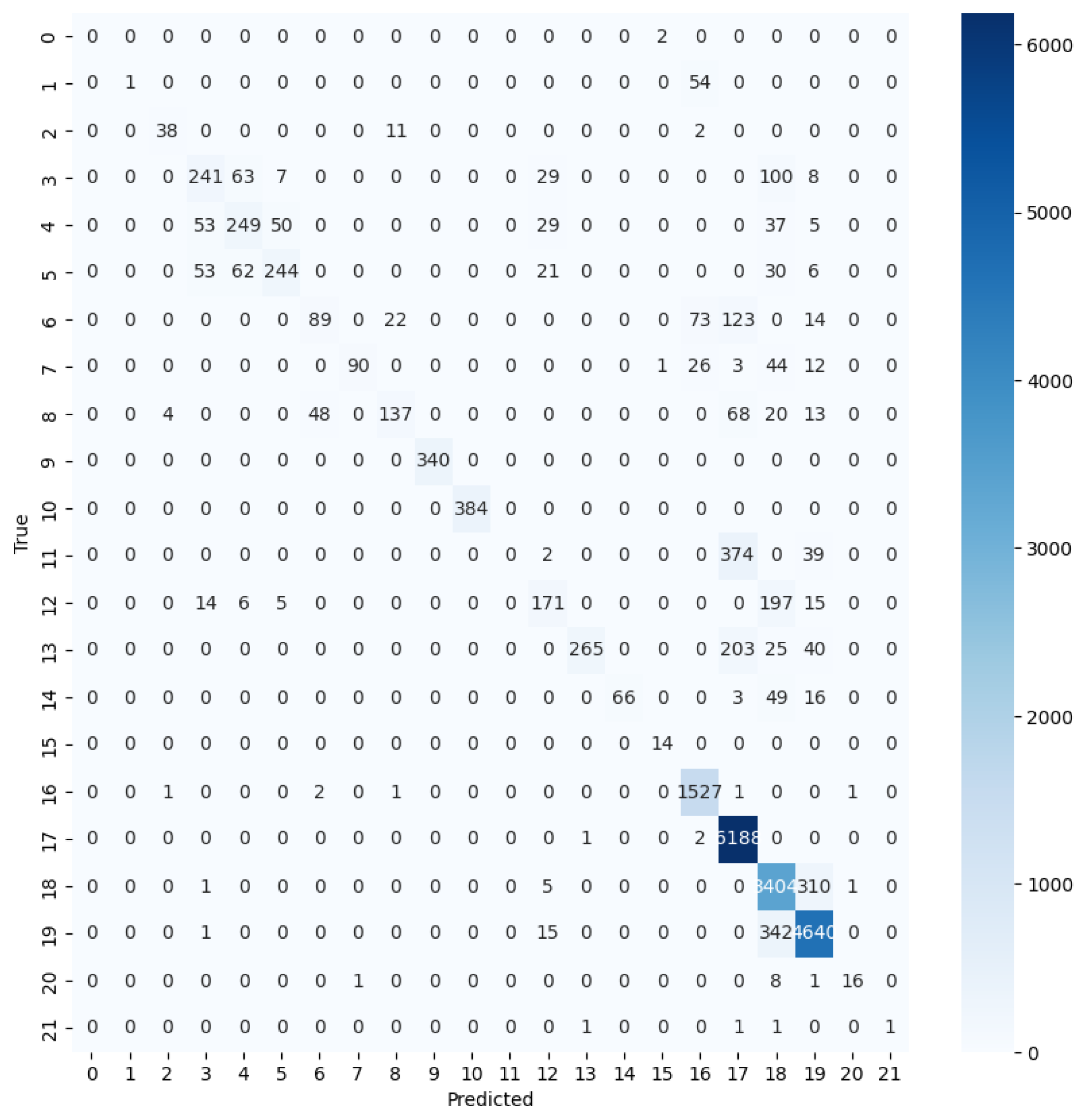
Figure 24.
The amount of dedicated time and estimated distribution (red line).
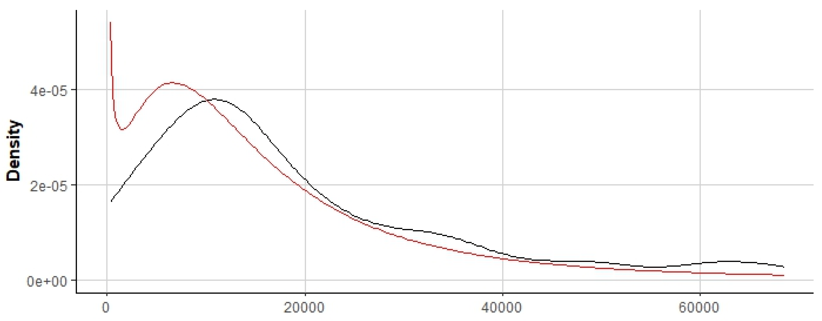
Table 2.
Introduction of event log activities.
| Activity Type | Notes | Activity Name | Activity Description |
| A | This refers to the loan’s states. A customer requests a loan, and Bank users and resources follow the activities to complete the process. | A_SUBMITTED | Initial request submission |
| The customer submits part of the required information for the loan request. | A_PARTLYSUBMITTED | Partial initial request submission | |
| The loan is pre-accepted but requires additional information. | A_PREACCEPTED | Pre-accepted | |
| The loan is accepted and under review for completeness. | A_ACCEPTED | Accepted | |
| The loan is finalized for completion. | A_FINALIZED | Finalized | |
| The loan application has been reviewed and approved. | A_APPROVED | Approved | |
| The approved loan has been registered in the system. | A_REGISTERED | Registered | |
| The loan account has been activated and is ready for use. | A_ACTIVATED | Activated | |
| The status of unsuccessful program termination indicates that the loan application was either canceled by the customer or declined by the bank. | A_CANCELLED/A_DECLINED | Canceled/Declined | |
| O | Refers to proposed states that have been communicated to the customer. | O_SELECTED | Selected for receiving the loan |
| The bank has prepared a loan proposal and sent it to the customer. | O_PREPARED | Proposal prepared and sent to the applicant | |
| The loan proposal has been sent to the customer. | O_SENT | Proposal sent | |
| The customer has responded to the loan proposal. | O_SENT BACK | Proposal response received from the applicant | |
| The customer has accepted the loan proposal. | O_ACCEPTED | Approved | |
| The loan proposal was canceled before approval. | O_CANCELLED | Cancelled | |
| The bank declined the loan proposal. | O_DECLINED | Declined | |
| W | This refers to states of work items occurring during the approval process. These events mainly involve manual efforts by bank resources during the approval process. Events describe efforts at different stages of the application process. Follow up on incomplete leads. | W_Afhandelen leads | Follow up on incomplete leads after proposals are sent to qualified applicants. |
| Complete requests that were previously pre-accepted. | W_Completeren aanvraag | Complete previously accepted requests. | |
| Follow up with applicants after proposals have been sent to them to ensure they have all the necessary information and to answer any questions. | W_Nabellen offers | Follow up after sending proposals to qualified applicants | |
| Evaluate the loan application for completeness and accuracy. | W_Valideren aanvraag | Loan evaluation | |
| Search for and collect missing information or documents needed to complete the loan application evaluation. | W_Nabellen incomplete dossiers | Search for additional information during the evaluation stage. | |
| Review and investigate loan applications flagged for potential fraud. | W_Beoordelen fraude | Review suspected fraud cases. | |
| Make amendments to the terms and conditions of approved loan contracts as needed. | W_Wijzigen contractgegevens | Amend approved contracts |
Table 3.
Missing links between start and end events.
| Activity | Missing start | Missing end | ||
| Variant | Case | Variant | Case | |
| W_Afhandelen leads | 1 | 1 | 0 | 0 |
| W_Beoordelen fraude | 0 | 0 | 0 | 0 |
| W_Completeren aanvraag | 104 | 455 | 0 | 0 |
| W_Nabellen incomplete dossiers | 7 | 7 | 0 | 0 |
| W_Nabellen offertes | 454 | 571 | 1 | 1 |
| W_Valideren aanvraag | 6 | 6 | 2 | 2 |
Table 4.
lifecycle stages of activities.
| Step | Description |
| SCHEDULE | Indicates that a work item is scheduled to occur in the future |
| START | Indicates the opening/start of a work item |
| COMPLETE | Indicates the end/conclusion of a work item |
Table 5.
The division of the loan amount and its results.
| Requested Amount | Cases | A_APPROVED | A_DECLINED | A_CANCELLED |
| 0 - 9999 | 6095 | 771 (12.65%) | 4197 (68.86%) | 1127 (18.50%) |
| 10000 - 19999 | 3627 | 808 (22.28%) | 1928 (53.16%) | 891 (24.57%) |
| 20000 - 29999 | 1593 | 389 (24.42%) | 776 (48.71%) | 428 (26.87%) |
| 30000 - 39999 | 665 | 164 (24.66%) | 324 (48.72%) | 177 (26.62%) |
| 40000 - 49999 | 296 | 62 (20.95%) | 158 (53.38%) | 76 (25.68%) |
| 50000 - 59999 | 337 | 48 (14.24%) | 206 (61.13%) | 83 (24.63%) |
| 60000 - 100000 | 75 | 4 (5.4%) | 46 (61.34%) | 25 (33.26%) |
Table 7.
Total working time of each resource.
| Resource | Total Working Time (h) | Total Working Day |
| 112 | 3101.37 | 167 |
| 10972 | 1002.43 | 104 |
| 11169 | 987.62 | 85 |
| 10932 | 960.61 | 69 |
| 10609 | 838.98 | 101 |
| 10138 | 720.14 | 100 |
| 10809 | 585.42 | 101 |
| 11203 | 492.03 | 74 |
Table 8.
Frequency of classified items based on their final evaluation for each case.
| Resource | A_CANCELLED | Resource | A_APPROVED | Resource | A_DECLINED |
| 112 | 1004 | 112 | 3 | 112 | 3429 |
| 11203 | 108 | 10629 | 359 | 10910 | 244 |
| 11119 | 97 | 10609 | 335 | 11169 | 238 |
| 11180 | 95 | 10809 | 271 | 10609 | 206 |
| 11181 | 95 | 10972 | 518 | 11189 | 172 |
| 10861 | 85 | 10138 | 681 | 10138 | 156 |
| 10913 | 82 | 10779 | 2 | 10913 | 155 |
| 10909 | 76 | 11289 | 68 | 10861 | 137 |
| 11201 | 72 | 11339 | 9 | 10982 | 133 |
Table 9.
Resources that can perform three types of action.
| Resource | A_DECLINED | CANCELLED | A_APPROVED |
| 112 | 3429 | 1004 | 3 |
| 10779 | 3 | 11 | 2 |
| 11339 | 1 | 0 | 9 |
| 11289 | 55 | 3 | 68 |
| 10138 | 156 | 5 | 681 |
| 10609 | 206 | 5 | 335 |
| 10809 | 87 | 1 | 271 |
| 10972 | 106 | 3 | 518 |
Table 10.
Frequency of end activities.
| Activity | Count |
| W_Valideren aanvraag | 2747 |
| W_Wijzigen contractgegevens | 4 |
| A_DECLINED | 3429 |
| W_Completeren aanvraag | 1939 |
| A_CANCELLED | 655 |
| W_Nabellen incomplete dossiers | 452 |
| W_Afhandelen leads | 2234 |
| W_Nabellen offertes | 1290 |
| W_Beoordelen fraude | 57 |
| O_CANCELLED | 279 |
| A_REGISTERED | 1 |
Table 11.
Miners’ performance comparison.
| Model | Average fitness | Precision | Generalization | Simplicity |
| Alpha Miner | 0.654 | 0.105 | 0.973 | 0.944 |
| Inductive Miner | 0.9887 | 0.129 | 0.947 | 0.611 |
| Heuristic Miner | 0.9888 | 0.314 | 0.954 | 0.5656 |
Disclaimer/Publisher’s Note: The statements, opinions and data contained in all publications are solely those of the individual author(s) and contributor(s) and not of MDPI and/or the editor(s). MDPI and/or the editor(s) disclaim responsibility for any injury to people or property resulting from any ideas, methods, instructions or products referred to in the content. |
© 2025 by the authors. Licensee MDPI, Basel, Switzerland. This article is an open access article distributed under the terms and conditions of the Creative Commons Attribution (CC BY) license (http://creativecommons.org/licenses/by/4.0/).
Copyright: This open access article is published under a Creative Commons CC BY 4.0 license, which permit the free download, distribution, and reuse, provided that the author and preprint are cited in any reuse.


