Particle Filtering Estimation of Regime Switching Factor Model and Its Application in Statistical Arbitrage Strategy

1. Introduction

Factor analysis plays a critical role in various areas of quantitative finance, including asset pricing, risk management, portfolio selection, and statistical arbitrage strategies, etc.. Broadly speaking, factor models can be categorized into two types: explicit factor models, which fall under supervised learning, and statistical factor models, which are typically unsupervised. Compared to explicit factor models such as Barra risk model [1], statistical factor models have two key advantages.

First, by construction, statistical factor models are more numerically stable and can capture the underlying covariance structure using fewer factors. Second, they are asset-class agnostic and therefore more broadly applicable across different markets. Given these strengths, this work focuses on the estimation and application of statistical factor models.

Statistical factor models has been developed as early as the 1930s. Scholars started to use factor models based on principal component analysis (PCA) back then [2]. PCA based factor models failed to provide a parametric model for the observations and perform poorly when within group variation dominates between group variation [3,4]. In the 1980s, maximum likelihood (ML) factor analysis estimated via the EM algorithm was introduced by Rubin and Thayer [5]. This was further generalized in the 1990s by Ghahramani and Hinton [6], who proposed the Mixture of Factor Analyzers. Their approach explains the hidden factors’ structure by combining clustering and local dimension reduction techniques. Mixture of factor analyzers works better than classical ML factor analysis due to its ability of segmenting data into different market regimes, each with its own factor structure. It handles the market regime changes in the covariance structure and hence has a more realistic assumption than the “one-size-fits-all” ML factor models.

Despite this advancement, within each regime, it still uses classical ML factor model which assumes i.i.d. hidden factors and Gaussian innovations. Dynamic factor model has a recursive structure for the hidden factor returns and can better model the factor return process [7,8,9,10]. This paper focus on the estimation of dynamic factor with regime switching factor loading that is governed by first order Markov Chain. The estimation relies on Particle filtering techniques [11,12], a class of Monte Carlo methods designed for solving the recursive Bayesian inference when analytical solutions such as the Kalman filter or Baum-Welch algorithm are infeasible.

Although particle filtering techniques is well developed when model parameter values are known, parameter learning in more complex settings remains challenging. Specifically, when parameters evolve according to a stochastic process rather than being constant, such as the applications in finance, an adaptive parameter learning algorithm becomes critical. To learn the parameter values, one early approach by Liu [13] incorporates parameters into the hidden state vector, but this often exacerbates the degeneracy issue in particle filtering. More computationally robust approaches have been introduced in [14,15]. Instead of combining parameter estimation to the learning algorithm they marginalize over parameters to reduce the estimation variance of their system. In this work, we implemented a particle filtering algorithm inspired by [14,15], and evaluate the estimation of regime switching dynamic factor model in the context of an equity statistical arbitrage strategy.

The rest of paper is organized as follows: Section 2 introduces the state space model and its estimation methods, including Kalman filter, EM algorithm, Particle filter, and the more recent development in the parameter learning - particle learning algorithm. Section 3 presents statistical factor models such as the MLE factor model, mixture of factor analyzers and the regime-switching dynamic factor model. We highlight the evolution of statistical factor models over recent decades and provides a simulation study demonstrating the effectiveness of particle learning algorithm for estimating the regime-switching dynamic factor model. Section 4 presents emprical studies applying the regime switching dynamic factor model in the context of equity stat-arb strategy and compares its performance to the conventional MLE factor model. Finally, Section 5 concludes the paper.

2. State Space Model and Its Estimation

A state space model is a framework used to describe the evolution of a dynamical system over time, particularly when the system is only partially observed. It has numerous applications in finance, such as time series prediction (alpha generation), statistical factor analysis (risk modeling), portfolio selection, etc.. In the most general form, a state space model can be represented by:

$$\begin{array}{cc}\hfill {\mathbf{x}}_t& =f_t\left({\mathbf{x}}_{t-1},{\mathbf{w}}_t\right)\hfill \end{array}$$

(1)

$$\begin{array}{cc}\hfill {\mathbf{y}}_t& =g_t\left({\mathbf{x}}_t,{\mathbf{v}}_t\right)\hfill \end{array}$$

(2)

where ${\mathbf{x}}_t$ denote the hidden states with dimension k, and ${\mathbf{y}}_t$ the observations with dimension s. The terms ${\mathbf{w}}_t$ and ${\mathbf{v}}_t$ represent the noise terms for the evolution equation $\left(1\right)$ and the observation equation $\left(2\right)$, with dimensions w and v respectively. The functions $f_t$ and $g_t$ are general nonlinear functions defining the state transition and observation processes. When the parameter values of the above equations are known, inference about the hidden states can be efficiently performed using the recursive Bayesian algorithm [12], which is summarized as Algorithm 1:

Algorithm 1 Recursive Bayesian Algorithm

Prediction: $$p\left({\mathbf{x}}_t\mid {\mathbf{y}}_{1:t-1}\right)=\int p\left({\mathbf{x}}_t\mid {\mathbf{x}}_{t-1}\right)p\left({\mathbf{x}}_{t-1}\mid {\mathbf{y}}_{1:t-1}\right)d{\mathbf{x}}_{t-1}$$ (3) Update: $$p\left({\mathbf{x}}_t\mid {\mathbf{y}}_{1:t}\right)={\displaystyle \frac{p\left({\mathbf{y}}_t\mid {\mathbf{x}}_t\right)p\left({\mathbf{x}}_t\mid {\mathbf{y}}_{1:t-1}\right)}{p\left({\mathbf{y}}_t\mid {\mathbf{y}}_{1:t-1}\right)}}$$ (4)

where the denominator in equation $\left(4\right)$ is another intergral needs to be solved in this problem:

$$p\left({\mathbf{y}}_t\mid {\mathbf{y}}_{1:t-1}\right)=\int p\left({\mathbf{y}}_t\mid {\mathbf{x}}_t\right)p\left({\mathbf{x}}_t\mid {\mathbf{y}}_{1:t-1}\right)d{\mathbf{x}}_t$$

(5)

2.1. Kalman Filter and Smoother

When the dynamical system described by equations $\left(1\right)$ and $\left(2\right)$ is linear, time-invariant, and finite-dimensional, functions $f_t$, and $g_t$ can be expressed in the following form:

$$\begin{array}{cc}\hfill {\mathbf{x}}_t& =\mathbf{B}{\mathbf{x}}_{t-1}+{\mathbf{w}}_t\hfill \end{array}$$

(6)

$$\begin{array}{cc}\hfill {\mathbf{y}}_t& =\mathbf{A}{\mathbf{x}}_t+{\mathbf{v}}_t\hfill \end{array}$$

(7)

and if we further assume ${\mathbf{w}}_t\sim N\left(0,\mathbf{Q}\right)$, ${\mathbf{v}}_t\sim N\left(0,\mathbf{R}\right)$, then Kalman filter can be derived to solve equations $\left(6\right)$ and $\left(7\right)$ analytically as described in [12] and Algorithm 2.

Algorithm 2 Kalman Filter

Prediction: $$\begin{array}{cc}\hfill {\mathbf{m}}_{t\mid t-1}& =\mathbf{B}{\mathbf{m}}_{t-1\mid t-1}\hfill \end{array}$$ (8) $$\begin{array}{cc}\hfill {\mathbf{C}}_{t\mid t-1}& =\mathbf{Q}+\mathbf{B}{\mathbf{C}}_{t-1\mid t-1}{\mathbf{B}}^T\hfill \end{array}$$ (9) Update: $$\begin{array}{cc}\hfill {\mathbf{m}}_{t\mid t}& ={\mathbf{m}}_{t\mid t-1}+{\mathbf{K}}_t\left({\mathbf{y}}_t-\mathbf{A}{\mathbf{m}}_{t\mid t-1}\right)\hfill \end{array}$$ (10) $$\begin{array}{cc}\hfill {\mathbf{C}}_{t\mid t}& ={\mathbf{C}}_{t\mid t-1}-{\mathbf{K}}_t\mathbf{A}{\mathbf{C}}_{t\mid t-1}\hfill \end{array}$$ (11)

where ${\mathbf{K}}_t$ is the Kalman gain and can be computed by:

$$\begin{array}{cc}\hfill {\mathbf{S}}_t& =\mathbf{A}{\mathbf{C}}_{t\mid t-1}{\mathbf{A}}^T+\mathbf{R}\hfill \end{array}$$

(12)

$$\begin{array}{cc}\hfill {\mathbf{K}}_t& ={\mathbf{C}}_{t\mid t-1}{\mathbf{A}}^T{\mathbf{S}}_t^{-1}\hfill \end{array}$$

(13)

When estimating hidden states in offline mode (i.e., when the full time series data is available) or when performing EM algorithm to estimate model parameters, the Kalman smoother is typically used to refine those state estimates using future observations as well (See Algorithm 3).

Algorithm 3 Kalman Smoother

$$\begin{array}{cc}\hfill {\mathbf{m}}_{t\mid T}& ={\mathbf{m}}_{t\mid t}+{\mathbf{K}}_{t\mid T}\left({\mathbf{m}}_{t+1\mid T}-\mathbf{B}{\mathbf{m}}_{t\mid t}\right)\hfill \end{array}$$ (14) $$\begin{array}{cc}\hfill {\mathbf{C}}_{t\mid T}& ={\mathbf{C}}_{t\mid t}+{\mathbf{K}}_{t\mid T}\left({\mathbf{C}}_{t+1\mid T}-{\mathbf{C}}_{t+1\mid t}\right){\mathbf{K}}_{t\mid T}^T\hfill \end{array}$$ (15)

where ${\mathbf{K}}_{t\mid T}={\mathbf{C}}_{t\mid t}{\mathbf{B}}^T{\mathbf{C}}_{t+1\mid t}^{-1}$ is the Kalman smoothing gain.

2.2. Parameter Estimation using EM algorithm

The Kalman filter algorithm introduced above assumes parameters of the system are known and fixed. When parameters are unknown, the EM algorithm [6] can be used to estimate these unknown parameters in a state-space form:

Algorithm 4 EM algorithm

E-Step: $$\begin{array}{cc}\hfill E\left[{\mathbf{x}}_t\mid {\mathbf{y}}_{1:T}\right]& ={\mathbf{m}}_{t\mid T}\hfill \end{array}$$ (16) $$\begin{array}{cc}\hfill E\left[{\mathbf{x}}_t{\mathbf{x}}_t^T\mid {\mathbf{y}}_{1:T}\right]& ={\mathbf{C}}_{t\mid T}+{\mathbf{m}}_{t\mid T}{\mathbf{m}}_{t\mid T}^T\hfill \end{array}$$ (17) $$\begin{array}{cc}\hfill E\left[{\mathbf{x}}_t{\mathbf{x}}_{t-1}^T\mid {\mathbf{y}}_{1:T}\right]& ={\mathbf{C}}_{t,t-1\mid T}+{\mathbf{m}}_{t\mid T}{\mathbf{m}}_{t-1\mid T}^T\hfill \end{array}$$ (18) M-Step: $$\begin{array}{cc}\hfill \widehat{\mathbf{A}}& =\left(\sum _{t=1}^T{\mathbf{y}}_{t}E{\left[{\mathbf{x}}_t\mid {\mathbf{y}}_{1:T}\right]}^T\right){\left(\sum _{t=1}^{T}E\left[{\mathbf{x}}_t{\mathbf{x}}_t^T\mid {\mathbf{y}}_{1:T}\right]\right)}^{-1}\hfill \end{array}$$ (19) $$\begin{array}{cc}\hfill \widehat{\mathbf{R}}& ={\displaystyle \frac{1}{T}}\sum _{t=1}^T\left({\mathbf{y}}_t{\mathbf{y}}_t^T-\widehat{\mathbf{A}}E\left[{\mathbf{x}}_t\mid {\mathbf{y}}_{1:T}\right]{\mathbf{y}}_t^T\right)\hfill \end{array}$$ (20) $$\begin{array}{cc}\hfill \widehat{\mathbf{B}}& =\left(\sum _{t=2}^{T}E\left[{\mathbf{x}}_t{\mathbf{x}}_{t-1}^T\mid {\mathbf{y}}_{1:T}\right]\right){\left(\sum _{t=2}^{T}E\left[{\mathbf{x}}_{t-1}\mid {\mathbf{y}}_{1:T}\right]\right)}^{-1}\hfill \end{array}$$ (21) $$\begin{array}{cc}\hfill \widehat{\mathbf{Q}}& ={\displaystyle \frac{1}{T-1}}\left(\sum _{t=2}^{T}E\left({\mathbf{x}}_t{\mathbf{x}}_t^T\mid {\mathbf{y}}_{1:T}\right)-\widehat{\mathbf{A}}\sum _{t=2}^{T}E\left[{\mathbf{x}}_t{\mathbf{x}}_{t-1}^T\mid {\mathbf{y}}_{1:T}\right]\right)\hfill \end{array}$$ (22) $$\begin{array}{cc}\hfill {\mathbf{m}}_1& =E\left[{\mathbf{x}}_1\mid {\mathbf{y}}_{1:T}\right]\hfill \end{array}$$ (23) $$\begin{array}{cc}\hfill {\mathbf{C}}_1& =E\left[{\mathbf{x}}_1{\mathbf{x}}_1^T\mid {\mathbf{y}}_{1:T}\right]-E\left[{\mathbf{x}}_1\mid {\mathbf{y}}_{1:T}\right]E{\left[{\mathbf{x}}_1\mid {\mathbf{y}}_{1:T}\right]}^T\hfill \end{array}$$ (24)

where ${\mathbf{m}}_{t\mid T}$, ${\mathbf{C}}_{t\mid T}$ will be estimated by Kalman filter and smoother. ${\mathbf{C}}_{t,t-1\mid T}$ can be updated by backward recursions:

$${\mathbf{C}}_{t,t-1\mid T}={\mathbf{C}}_{t\mid t}{\mathbf{K}}_{t-1\mid T}^T+{\mathbf{K}}_{t\mid T}\left({\mathbf{C}}_{t+1,t\mid T}-\mathbf{B}{\mathbf{C}}_{t\mid t}\right){\mathbf{K}}_{t-1\mid T}^T$$

(25)

which is initialized by ${\mathbf{C}}_{T,T-1\mid T}=\left(\mathbf{I}-{\mathbf{K}}_T\mathbf{A}\right)\mathbf{B}{\mathbf{C}}_{T-1\mid T-1}$.

2.3. Particle Filter

When the dynamical system $\left(1\right)$ and $\left(2\right)$ do not admit a linear-Gaussian representation as in $\left(6\right)$, and $\left(7\right)$, deriving an analytical solution for the recursive Bayesian inference becomes challenging. In such cases, particle filtering techniques has been a very popular approach for solving nonlinear dynamical system, including models like the stochastic volatility model [14]. In this section, we introduce several baseline particle filtering algorithms.

2.3.1. SIS Particle Filter

Sequential Importance Sampling (SIS) particle filter has been introduced as early as 1990s [16]. The main idea is to approximate the joint posterior density at time t using importance sampling method:

$$p\left({\mathbf{x}}_{1:t}\mid {\mathbf{y}}_{1:t}\right)\approx \sum _{i=1}^N{W}_t^i\delta \left({\mathbf{x}}_{1:t}-{\mathbf{x}}_{1:t}^i\right)$$

(26)

where $\delta \left(·\right)$ is the Dirac delta function, and $W_t^i$ is the importance weight for particle i, given by:

$$W_t^i\propto {\displaystyle \frac{p\left({\mathbf{x}}_{1:t}\mid {\mathbf{y}}_{1:t}\right)}{q\left({\mathbf{x}}_{1:t}\mid {\mathbf{y}}_{1:t}\right)}}$$

(27)

where $p\left({\mathbf{x}}_{1:t}\mid {\mathbf{y}}_{1:t}\right)$ is the target distribution and $q\left({\mathbf{x}}_{1:t}\mid {\mathbf{y}}_{1:t}\right)$ is the importance (or proposal) distribution. A sequential estimation algorithm can be derived if we assume the joint importance density has the following factorization:

$$q\left({\mathbf{x}}_{1:t}\mid {\mathbf{y}}_{1:t}\right)=q\left({\mathbf{x}}_t\mid {\mathbf{x}}_{t-1},{\mathbf{y}}_t\right)q\left({\mathbf{x}}_{1:t-1}\mid {\mathbf{y}}_{1:t-1}\right)$$

(28)

This factorization allows sequential sampling of the state ${\mathbf{x}}_t$ given the previous state and current observation, which forms the foundation of the SIS particle filter as in Algorithm 5:

Algorithm 5 SIS Particle Filter

Draw ${\mathbf{x}}_t^i\sim q\left({\mathbf{x}}_t\mid {\mathbf{x}}_{t-1}^i,{\mathbf{y}}_t\right)$ Assign the particle ${\mathbf{x}}_t^i$ a weight, $W_t^i\propto W_{t-1}^i{\displaystyle \frac{p\left({\mathbf{y}}_t\mid {\mathbf{x}}_t^i\right)p\left({\mathbf{x}}_t^i\mid {\mathbf{x}}_{t-1}^i\right)}{q\left({\mathbf{x}}_t^i\mid {\mathbf{x}}_{t-1}^i,{\mathbf{y}}_t\right)}}$

2.3.2. SIR Particle Filter

The SIS particle filter often fails in practice due to the weight degeneracy issue. The variance of the weight $W_t^i$ in SIS filter will increase over time until only one particle left with large weight. To alleviate this issue, we can resample (with replacement) the particles based on their weights. By doing so we can replicate those particles with large weights, eliminate particles with small weights, and hence reduce the variance of weights $W_t^i$ [11].

Moreover, It has been shown the optimal importance density for a generic particle filter algorithm is $p\left({\mathbf{x}}_t\mid {\mathbf{x}}_{t-1}^i,{\mathbf{y}}_t\right)$ [17] and if we are able to choose the importance density close to the optimal importance density we can further alleviate the weight degeneracy issue. SIR particle filter uses $p\left({\mathbf{x}}_t\mid {\mathbf{x}}_{t-1}^i\right)$ as important density and applying resampling at each step as shown in the Algorithm 6:

Algorithm 6 SIR Particle Filter

Draw ${\mathbf{x}}_t^i\sim p\left({\mathbf{x}}_t\mid {\mathbf{x}}_{t-1}^i\right)$ Assign the particle ${\mathbf{x}}_t^i$ a weight, $W_t^i\propto p\left({\mathbf{y}}_t\mid {\mathbf{x}}_t^i\right)$ Resampling based on weight $W_t^i$

Although SIR filter improves the weight degeneracy problem present in the SIS filter, it still has its own weakness [18]. First, if there is an outlier at time t, the weights $W_t^i$ will unevenly distributed and the filter will become imprecise. Second, the predictive density $p\left({\mathbf{x}}_t\mid {\mathbf{x}}_{t-1}^i\right)$ often fails to capture tail behavior accurately, causing some particles to drift into low-likelihood regions during the prediction step (2).

2.3.3. Auxiliary Particle Filter

To address the limitations of the SIR filter, the auxiliary particle filter proposed by [18] introduces a lookahead step - also known as the auxiliary variable mechanism. This approach uses a predictive weighting scheme (See Algorithm 7 step 1) that estimates the likelihood of the upcoming observation given the predicted state, a process often referred to as lookahead weighting.

Algorithm 7 Auxiliary Particle Filter

(Resample) Draw $k^i\sim Multi\left\{W_t^1,\dots ,W_t^N\right\},$where $W_t^i\propto p\left({\mathbf{y}}_t\mid \mu \left({\mathbf{x}}_{t-1}^i\right)\right)$. (Propagate) Draw ${\tilde{\mathbf{x}}}_t^i\sim p\left({\mathbf{x}}_t\mid {\mathbf{x}}_{t-1}^{k^i}\right)$. (Resample) Draw ${\mathbf{x}}_t^i\sim Multi\left\{W_t^1,\dots ,W_t^N\right\}$, where $W_t^t\propto p\left({\mathbf{y}}_t\mid {\tilde{\mathbf{x}}}_t^i\right)/p\left({\mathbf{y}}_t\mid \mu \left({\mathbf{x}}_{t-1}^i\right)\right)$.

where $\mu \left({\mathbf{x}}_{t-1}^i\right)$ denotes the mean, median, or mode of the distribution of ${\mathbf{x}}_t$ given ${\mathbf{x}}_{t-1}^i$. When the observation equation is informative in dynamical system, Auxiliary particle filter usually will reduce variance in particle weights and hence perform better.

2.4. Particle Filter with Parameter Learning

The particle filter algorithms discussed so far assume that model parameters are known. However, in many applications, model parameters are typically unknown. Learning the static parameter values - or more broadly - identifying the coefficient evolution process - is a critical aspect of system identification. The integration of parameter learning into the particle filtering framework has been extensively studied [19].

One idea is to treat parameters as additional hidden state variables in the particle filtering framework, but this approach often leads to severe degeneracy issue. To address this issue, [13] proposed introducing an artificial evolutional model for the parameters and augment the hidden state space by including them.

Another idea is to integrate out (or marginalize out) the parameters whenever feasible [14,20,21]. The benefits of the marginalized particle filter has been discussed in [22].

Building on these ideas, Carvalho et al. [15] introduced particle learning approach, a noval particle filter with the embedded parameter learning step. Particle learning method marginalize both the parameters and the hidden states by tracking only the sufficient statistics of them, which updated later using recursive Bayesian algorithm and Kalman filter, respectively. It is also constructed under the Auxiliary particle filter framework, and the performance improvement has been demonstrated in [15,23].

In our paper, we develop a simplified version of the particle learning algorithm to estimate regime switching dynamic factor model.

2.4.1. Particle Learning

Particle learning algorithm was introduced by Carvalho et al. in [15], extending the idea of auxiliary particle filter to incorporate parameter learning. While the overall filtering scheme is the same as auxiliary particle filter. the key innovation lies in tracking the “essential state” ${\mathbf{z}}_t$.

Specifically, ${\mathbf{z}}_t$ includes:

• the sufficient statistics of the parameter vector ${\mathbf{s}}_t$,
• the sufficient statistics of hidden states ${\mathbf{x}}_t$, ${\mathbf{s}}_t^x$, and
• the current value of the parameter vector, ${\theta }_t$:

  $${\mathbf{z}}_t=\left\{{\mathbf{s}}_t,{\mathbf{s}}_t^x,{\theta }_t\right\}.$$

The reason we include parameter value in essential state is because for evaluating likelihood and drawing samples from predictive density we need to use parameter values. However, there values are not directly sampled at each step, which most likely will cause degeneracy issue; instead, they are inferred offline from their associated sufficient statistics. This approach is also referred to as marginalization by simulation.

The derivation of this filter start with the recursive relation:

$$p\left({\mathbf{z}}_t\mid {\mathbf{y}}_{1:t}\right)\propto \int p\left({\mathbf{y}}_t\mid {\mathbf{z}}_{t-1}\right)p\left({\mathbf{z}}_t\mid {\mathbf{z}}_{t-1},{\mathbf{y}}_t\right)p\left({\mathbf{z}}_{t-1}\mid {\mathbf{y}}_{1:t-1}\right)d{\mathbf{z}}_{t-1}$$

where

$$\begin{array}{c}p\left({\mathbf{z}}_t\mid {\mathbf{z}}_{t-1},{\mathbf{y}}_t\right)=\int p\left({\mathbf{s}}_t\mid {\mathbf{s}}_{t-1},{\mathbf{x}}_t,{\mathbf{y}}_t\right)p\left({\mathbf{s}}_t^x\mid {\mathbf{s}}_{t-1}^x,{\mathbf{x}}_t,{\mathbf{y}}_t\right)\\ ·p\left({\mathbf{x}}_t\mid {\mathbf{s}}_{t-1}^x,{\mathbf{y}}_t\right)d{\mathbf{x}}_t\end{array}$$

and

$$p\left({\mathbf{x}}_t\mid {\mathbf{s}}_{t-1}^x,{\mathbf{y}}_t\right)=\int p\left({\mathbf{x}}_t\mid {\mathbf{x}}_{t-1},{\mathbf{y}}_t\right)p\left({\mathbf{x}}_{t-1}\mid {\mathbf{s}}_{t-1}^x,{\mathbf{y}}_t\right)d{\mathbf{x}}_{t-1}$$

So given the particles of ${\mathbf{s}}_{t-1}^x$ we can construct Monte Carlo estimate for $p\left({\mathbf{x}}_t\mid {\mathbf{s}}_{t-1}^x,{\mathbf{y}}_t\right)$ by sampling from $p\left({\mathbf{x}}_{t-1}\mid {\left({\mathbf{s}}_{t-1}^x\right)}^i,{\mathbf{y}}_t\right)$ and $p\left({\mathbf{x}}_t\mid {\mathbf{x}}_{t-1}^i,{\mathbf{y}}_t\right)$ respectively. After that we can update ${\mathbf{s}}_t$ and ${\mathbf{s}}_t^x$ deterministically. Particle learning method can be summarized as follows:

Algorithm 8 Particle Learning

(Resample) Draw $k^i\sim Multi\left\{W_t^1,\dots ,W_t^N\right\}$, where $W_t^i\propto p\left({\mathbf{y}}_t\mid {\mathbf{z}}_{t-1}^i\right)$ (Propagate) Draw ${\mathbf{x}}_{t-1}^i\sim p\left({\mathbf{x}}_{t-1}\mid {\left({\mathbf{s}}_{t-1}^x\right)}^{k^i},{\theta }_{t-1}^{k^i},{\mathbf{y}}_t\right)$ (Propagate) Draw ${\mathbf{x}}_t^i\sim p\left({\mathbf{x}}_t\mid {\mathbf{x}}_{t-1}^i,{\theta }_{t-1}^{k^i},{\mathbf{y}}_t\right)$ (Update) ${\mathbf{s}}_t^i=\mathcal{S}\left({\mathbf{s}}_{t-1}^{k^i},{\mathbf{x}}_t^i,{\mathbf{x}}_{t-1}^i,{\mathbf{y}}_t\right)$ (Sample) Draw ${\theta }_t^i\sim p\left({\theta }_t\mid {\mathbf{s}}_t^i\right)$ (Update) ${\left({\mathbf{s}}_t^x\right)}^i=\mathcal{K}\left({\left({\mathbf{s}}_{t-1}^x\right)}^{k^i},{\theta }_t^i,{\mathbf{y}}_t\right)$

Where $\mathcal{S}$ denotes the deterministic updating function for parameter sufficient statistics and $\mathcal{K}$ denotes Kalman filter for state sufficient statistics update.

3. Statistical Factor Analysis

Statistical factor analysis is a technique used to explain the correlation structure of multivariate observations through a lower-dimensional set of unobserved factors. The model can be expressed as:

$${\mathbf{y}}_t=\mathbf{B}{\mathbf{x}}_t+{\mathbf{v}}_t$$

(29)

where ${\mathbf{y}}_t$ is $\left(s\times 1\right)$ vector of observations, ${\mathbf{x}}_t$ is $\left(k\times 1\right)$ vector of statistical factors, and $\mathbf{B}$ is $\left(s\times k\right)$ factor loading matrix. ${\mathbf{v}}_t$ is the $\left(s\times 1\right)$ error term that follows certain distribution assumption. The hidden factors ${\mathbf{x}}_t$ are often assumed to follow an i.i.d. standard normal distribution, i.e. ${\mathbf{x}}_t\sim N\left(0,{\mathbf{I}}_k\right)$, and are assumed to be independent of the error term ${\mathbf{v}}_t$.

3.1. MLE Factor Analsis

The most commonly used approach for estimating the factor model in equation $\left(29\right)$ is the Expectation-Maximization (EM) algorithm for maximum likelihood estimation (MLE) [4,5,6]. The EM algorithm for maximum likelihood estimation of the factor model is outlined below as Algorithm 9:

Algorithm 9 EM algorithm for Statistical Factor Analysis

E-Step: Given current fit of $\mathbf{B}$ and $\mathbf{R}$, calculate sufficient statistics: $$\begin{array}{cc}\hfill \gamma & ={\mathbf{B}}^T{\left(\mathbf{B}{\mathbf{B}}^T+\mathbf{R}\right)}^{-1}\hfill \end{array}$$ (30) $$\begin{array}{cc}\hfill E\left[{\mathbf{x}}_t\mid {\mathbf{y}}_t\right]& =\gamma {\mathbf{y}}_t\hfill \end{array}$$ (31) $$\begin{array}{cc}\hfill E\left[{\mathbf{x}}_t{\mathbf{x}}_t^T\mid {\mathbf{y}}_t\right]& =\mathbf{I}-\gamma \mathbf{B}+\gamma {\mathbf{y}}_t{\mathbf{y}}_t^T\gamma \hfill \end{array}$$ (32) M-Step: Update parameter estimation, $$\begin{array}{cc}\hfill \widehat{\mathbf{B}}& =\left(\sum _{t=1}^T{\mathbf{y}}_{t}E\left[{\mathbf{x}}_t\mid {\mathbf{y}}_t\right]\right){\left(\sum _{t=1}^{T}E\left[{\mathbf{x}}_t{\mathbf{x}}_t^T\mid {\mathbf{y}}_t\right]\right)}^{-1}\hfill \end{array}$$ (33) $$\begin{array}{cc}\hfill \widehat{\mathbf{R}}& ={\displaystyle \frac{1}{T}}\mathrm{diag}\left(\sum _{t=1}^T\left({\mathbf{y}}_t{\mathbf{y}}_t^T-\widehat{\mathbf{B}}E\left[{\mathbf{x}}_t\mid {\mathbf{y}}_t\right]{\mathbf{x}}_t^T\right)\right)\hfill \end{array}$$ (34)

The EM algorithm starts with certain initial values for $\mathbf{B}$ and $\mathbf{R}$ and terminates when the rate of change in the log likelihood falls below some critical value. The log likelihood can be computed as:

$$\begin{array}{ccc}\hfill logL\left(\mathbf{B},\mathbf{R}\mid {\mathbf{y}}_{1:T}\right)& =& -{\displaystyle \frac{1}{2}}\left(\phantom{\sum _{t=1}^T}\right.T\left(slog\left(2\pi \right)+log\left(det\left(\mathbf{B}{\mathbf{B}}^T+\mathbf{R}\right)\right)\right)\hfill \\ & & +\sum _{t=1}^T{\mathbf{y}}_t^T{\left(\mathbf{B}{\mathbf{B}}^T+\mathbf{R}\right)}^{-1}{\mathbf{y}}_t\left.\phantom{\sum _{t=1}^T}\right)\hfill \end{array}$$

(35)

3.2. Mixture of Factor Analyzer

The factor model in equation $\left(29\right)$ is a global linear model. However, in many real world applications — such as in financial engineering — it fails to reflect the fact that the observed data present multiple regimes whose behaviors differ materially. To address this limitation, the Mixture of Factor Analyzer (MFA) model extends the MLE statistical factor model by combining local dimension reduction method with a Gaussian mixture model for clustering. Specifically, the MFA model can be described in the following form:

$${\mathbf{y}}_t=\mathbf{B}\left(i\right){\mathbf{x}}_t+{\mathbf{v}}_t\mathrm{with}\mathrm{prob}.{\pi }_i\left(i=1,\dots ,m\right)$$

(36)

where ${\sum }_{i=1}^m{\pi }_i=1,{\pi }_i\ge 0$ , and the index i denotes the component (or regime), drawn from a categorical distribution with mixing probabilities $\left\{{\pi }_i\right\}$. $\mathbf{B}\left(i\right)$ is the factor loading matrix specific to component i. Following the formulation in [6], we assume the observation covariance $\mathbf{R}$ for each component are the same, and the number of mixture is fixed prior to the estimation step. The EM algorithm for estimating the parameters of the MFA model is described below in Algorithm 10:

Algorithm 10 EM algorithm for Mixture of Factor Analyzer

E-Step: Given current fit of ${\pi }_i\mathrm{for}i=1,\dots ,m$, $\mathbf{B}$ and $\mathbf{R}$, calculate, $$\begin{array}{ccc}\hfill {\tau }_{ij}& =& {\displaystyle \frac{{\pi }_{i}N\left({\mathbf{y}}_j,\mathbf{B}\left(i\right)\mathbf{B}{\left(i\right)}^T+\mathbf{R}\right)}{{\sum }_{i=1}^m{\pi }_{i}N\left({\mathbf{y}}_j,\mathbf{B}\left(i\right)\mathbf{B}{\left(i\right)}^T+\mathbf{R}\right)}}\hfill \end{array}$$ (37) $$\begin{array}{ccc}\hfill \gamma \left(i\right)& =& \mathbf{B}{\left(i\right)}^T{\left(\mathbf{B}\left(i\right)\mathbf{B}{\left(i\right)}^T+\mathbf{R}\right)}^{-1}\hfill \end{array}$$ (38) $$\begin{array}{ccc}\hfill \Sigma \left(i\right)& =& {\displaystyle \frac{1}{T}}\sum _{j=1}^T\left(\sqrt{{\tau }_{ij}}{\mathbf{y}}_j\right){\left(\sqrt{{\tau }_{ij}}{\mathbf{y}}_j\right)}^T\hfill \end{array}$$ (39) M-Step: $$\begin{array}{ccc}\hfill \widehat{\mathbf{B}}\left(i\right)& =& {\displaystyle \frac{\Sigma \left(i\right)\gamma {\left(i\right)}^T}{\frac{1}{T}{\sum }_{j=1}^T{\tau }_{ij}\left({\mathbf{I}}_s-\gamma \left(i\right)\mathbf{B}\left(i\right)\right)+\gamma \left(i\right)\Sigma \left(i\right)\gamma {\left(i\right)}^T}}\hfill \end{array}$$ (40) $$\begin{array}{ccc}\hfill \widehat{\mathbf{R}}& =& {\displaystyle \frac{1}{T}}\mathrm{diag}\left(\sum _{i=1}^m\Sigma \left(i\right)-\sum _{i=1}^m\widehat{\mathbf{B}}\left(i\right)\gamma \left(i\right)\Sigma \left(i\right)\right)\hfill \end{array}$$ (41) $$\begin{array}{ccc}\hfill {\widehat{\pi }}_i& =& {\displaystyle \frac{1}{T}}\sum _{j=1}^T{\tau }_{ij}\hfill \end{array}$$ (42)

Starting with initial values of ${\pi }_i$ for $i=1,\dots ,m$, $\mathbf{B}\left(i\right)$, and $\mathbf{R}$, we can iterate algorithm 10 until convergence. The log-likelihood of the observed data under the MFA model is given by:

$$logL\left(\mathbf{\Psi }\right)=\sum _{j=1}^{T}log\left\{\sum _{i=1}^m{\pi }_{i}N\left({\mathbf{y}}_j,\mathbf{B}\left(i\right)\mathbf{B}{\left(i\right)}^T+\mathbf{R}\right)\right\}$$

where $\mathbf{\Psi }$ denotes the set of all model parameters.

3.3. Regime Switching Dynamic Factor Model

Although the mixture of factor analyzer (MFA) model can capture data generated from multiple regimes, it still assumes the observations are i.i.d. and fails to account for the temporal persistence of market regimes. In practice, particularly in financial applications, market regimes tend to persist over time, with each regime exhibiting distinct statistical properties. Regime switching model equipped with Markov chain mechanism can better model the regime persistence and capture the abrupt regime shifts more efficiently than commonly used “low-pass filtering” approaches such as rolling window estimation. It fits better for financial time series, where capturing time dynamics is essential.

3.3.1. Methods

In this work, we represent the regime switching dynamic factor model within a state space framework. The estimation of regime switching state space models has been well studied in the literature [8,24,25], with most approaches relying on the Markov Chain Monte Carlo (MCMC) algorithms. MCMC approaches are not only computationally very expensive, but also suffer slow convergence issue. Moreover, they are batch (offline) algorithms in nature which limits their use in real-time trading.

In this work, we will rely on the particle learning technique that is introduced in section 2.4 as our estimation method. Computationally, it’s significantly faster than MCMC algorithms and, being an online algorithm, it can be adopted in the real time trading environment. The convergence of particle filtering algorithm is well studied in the literature [17,26].

Another key advantage of the particle filtering framework is its modular design, which makes it highly adaptable to complex model structures. Additional structure can be incorporated into the system relatively easier than MCMC framework, as long as it remains possible to draw samples from the importance density and evaluate the likelihood function upon receiving the new observations (See [14,27] for examples).

To introduce our model, we first define a discrete latent regime variable $r_t\in \left\{1,\dots ,K\right\}$ which captures the regime at time t. The essential state used in the particle learning algorithm is then extended as:

$${\mathbf{Z}}_t=\left\{r_t,{\mathbf{s}}_t,{\mathbf{s}}_t^x,\theta \right\},$$

where ${\mathbf{s}}_t$ and ${\mathbf{s}}_t^x$ denote the sufficient statistics for the parameters and the hidden states, respectively, and $\theta$ denotes the model parameters.

The model is specified as:

$$\begin{array}{cc}\hfill {\mathbf{x}}_t& =\mathbf{A}{\mathbf{x}}_t+{\mathbf{w}}_t\hfill \end{array}$$

(43)

$$\begin{array}{cc}\hfill {\mathbf{y}}_t& =B\left(r_t\right){\mathbf{x}}_t+\sqrt{{\lambda }_t}{\mathbf{v}}_t\hfill \end{array}$$

(44)

$$\begin{array}{cc}\hfill {\lambda }_t& \sim IG\left(v/2,v/2\right)\hfill \end{array}$$

(45)

where $IG\left(·\right)$ denotes the inverse Gamma distribution, ${\mathbf{v}}_t\sim N\left(0_s,{\mathbf{R}}_s\right)$, ${\mathbf{w}}_t\sim N\left(0_k,{\mathbf{I}}_k\right)$. In this representation, we model heavy tailed innovation using the data augmentation scheme of [28], where at each time t, we will follow the two step approach: i) ${\lambda }_t\sim \mathrm{Inv}-\mathrm{Gamma}\left(v/2,v/2\right)$, ii) ${\eta }_t={\sqrt{\lambda }}_t{\mathbf{v}}_t$, so that ${\eta }_t\sim t_v\left(0_s,{\mathbf{R}}_s\right)$ where ${\mathbf{R}}_s$ is a diagonal matrix.

If the degree of freedom is given, the at each time step t, our system is a conditionally Gaussian model. To derive the particle learning algorithm for this model (equation $\left(43\right)$ to $\left(45\right)$), we compute the predictive density $p\left({\mathbf{y}}_t\mid {\mathbf{z}}_{t-1},{\lambda }_t\right)$ by integrating out the latent regime variable $r_t$:

$$\begin{array}{ccc}\hfill p\left({\mathbf{y}}_t\mid {\mathbf{z}}_{t-1},{\lambda }_t\right)& =& \sum _{r_t=1}^{K}p\left({\mathbf{y}}_t\mid r_t,{\left({\mathbf{s}}_{t-1}^x,\theta ,{\lambda }_t\right)}^i\right)\hfill \\ & & ·p\left(r_t\mid r_{t-1},\theta \right)\hfill \end{array}$$

(46)

where $p\left({\mathbf{y}}_t\mid r_t,{\left({\mathbf{s}}_{t-1}^x,\theta ,{\lambda }_t\right)}^i\right)$ is the conditional likelihood, which is derived in Appendix A, and $p\left(r_t\mid r_{t-1},\theta \right)$ is given by the estimated transition matrix. To propagate $r_t$, we sample from the posterior distribution:

$$\begin{array}{ccc}\hfill p\left(r_t\mid {\left(r_{t-1},{\mathbf{s}}_{t-1}^x,\theta ,{\lambda }_t\right)}^i,{\mathbf{y}}_t\right)& \propto & p\left({\mathbf{y}}_t\mid r_t,{\left({\mathbf{s}}_{t-1}^x,\theta ,{\lambda }_t\right)}^i\right)\hfill \\ & & ·p\left(r_t\mid r_{t-1},\theta \right)\hfill \end{array}$$

(47)

Algorithm 11 PL for Regime Switching Dynamic Factor Model

(Sampling) Draw ${\lambda }_t^i\sim IG\left(v/2,v/2\right)$ (${\lambda }_t^i=1$ for Gaussian model) (Resample) Draw $k^i\sim Multi\left\{W_t^1,\dots ,W_t^N\right\}$, with $W_t^i\propto p\left({\mathbf{y}}_t\mid {\mathbf{z}}_{t-1}^i,{\lambda }_t\right)$ where $$p\left({\mathbf{y}}_t\mid {\mathbf{z}}_{t-1}^i,{\lambda }_t\right)=\sum _{k=1}^{K}N\left({\mathbf{y}}_t;{\mathbf{m}}_y\left(k\right),{\mathbf{C}}_y\left(k\right)\right)p\left(r_t=k\mid r_{t-1}^i,\theta \right)$$ and ${\mathbf{m}}_y\left(k\right)=\mathbf{B}\left(k\right)\mathbf{A}{\mathbf{m}}_{t-1}$, ${\mathbf{C}}_y\left(k\right)=\mathbf{B}\left(k\right)\mathbf{A}{\mathbf{C}}_{t-1}{\mathbf{A}}^T\mathbf{B}{\left(k\right)}^T+\mathbf{B}\left(k\right)\mathbf{B}{\left(k\right)}^T+{\lambda }_t{\mathbf{R}}_s$. (Propagate) Draw $r_t^i\sim p\left(r_t\mid {\left({\mathbf{s}}_{t-1}^x,r_{t-1},\theta \right)}^{k^i},{\mathbf{y}}_t\right)$, which follows multinomial distribution with: $$p\left(r_t=k\mid {\mathbf{s}}_{t-1}^x,r_{t-1},\theta ,{\mathbf{y}}_t\right)\propto N\left({\mathbf{y}}_t;{\mathbf{m}}_y^{k^i}\left(k\right),{\mathbf{C}}_y^{k^i}\left(k\right)\right)p\left(r_t=k\mid r_{t-1}^{k^i},{\theta }^{k^i}\right)$$ (Propagate) Draw ${\mathbf{x}}_t^i\sim p\left({\mathbf{x}}_t\mid r_t^i,{\mathbf{x}}_{t-1}^{k^i},{\theta }^{k^i},{\mathbf{y}}_t\right)$ from normal distribution $N\left({\mathbf{m}}_x,{\mathbf{C}}_x\right)$ with: $$\begin{array}{ccc}\hfill {\mathbf{m}}_x& =& {\mathbf{C}}_x\left(\mathbf{B}{\left(r_t\right)}^T{\left({\lambda }_t{\mathbf{R}}_s\right)}^{-1}{\mathbf{y}}_t+\mathbf{A}{\mathbf{x}}_{t-1}\right)\hfill \end{array}$$ (48) $$\begin{array}{ccc}\hfill {\mathbf{C}}_x^{-1}& =& \mathbf{B}{\left(r_t\right)}^T{\left({\lambda }_t{\mathbf{R}}_s\right)}^{-1}\mathbf{B}\left(r_t\right)+{\mathbf{I}}_k\hfill \end{array}$$ (49) (Update) ${\mathbf{s}}_t^i=\mathbf{S}\left({\mathbf{s}}_{t-1}^{k^i},r_t^i,r_{t-1}^{k^i},{\mathbf{x}}_t^i,{\mathbf{x}}_{t-1}^{k^i},{\mathbf{y}}_t\right)$. (Sample) Draw ${\theta }^i\sim p\left(\theta \mid {\mathbf{s}}_t^i\right)$. (Update) ${\left({\mathbf{s}}_t^x\right)}^i=\mathbf{K}\left({\left({\mathbf{s}}_{t-1}^x\right)}^{k^i},{\theta }^i,{\mathbf{y}}_t\right)$ and draw estimated states ${\widehat{\mathbf{x}}}_t^i\sim N\left({\mathbf{m}}_{x1}^i,{\mathbf{C}}_{x1}^i\right)$.

where the deterministic updating formula $\mathbf{S}$ in step 5 is given by:

$$\begin{array}{ccc}\hfill v_t& =& {\phi }^2{v}_{t-1}+1\hfill \end{array}$$

(50)

$$\begin{array}{ccc}\hfill {\mathbf{g}}_t& =& {\mathbf{\Phi }}_{t-1}{\mathbf{x}}_t\hfill \end{array}$$

(51)

$$\begin{array}{ccc}\hfill {\zeta }_t^2& =& {\lambda }_t{\phi }^2+{\mathbf{x}}_t^T{\mathbf{g}}_t\hfill \end{array}$$

(52)

$$\begin{array}{ccc}\hfill {\widehat{\mathbf{e}}}_t& =& {\mathbf{y}}_t-{\mathbf{b}}_{t-1}^T{\mathbf{x}}_t\hfill \end{array}$$

(53)

$$\begin{array}{ccc}\hfill {\mathbf{b}}_t& =& {\mathbf{b}}_{t-1}+{\displaystyle \frac{1}{{\zeta }_t^2}}{\mathbf{g}}_t{\widehat{\mathbf{e}}}_t^T{I}_{r_t=k}\hfill \end{array}$$

(54)

$$\begin{array}{ccc}\hfill {\mathbf{\Phi }}_t& =& {\displaystyle \frac{1}{{\phi }^2}}\left({\mathbf{\Phi }}_{t-1}-{\displaystyle \frac{1}{{\zeta }_t^2}}{\mathbf{g}}_t{\mathbf{g}}_t^T{I}_{r_t=k}\right)\hfill \end{array}$$

(55)

$$\begin{array}{ccc}\hfill {\mathbf{V}}_t& =& {\phi }^2\left({\mathbf{V}}_{t-1}+\sum _{k=1}^K{\displaystyle \frac{1}{{\zeta }_t^2}}{\widehat{\mathbf{e}}}_t{\widehat{\mathbf{e}}}_t^T{I}_{r_t=k}\right)\hfill \end{array}$$

(56)

$$\begin{array}{ccc}\hfill {\mathbf{g}}_t^x& =& {\mathbf{\Psi }}_{t-1}{\mathbf{x}}_{t-1}\hfill \end{array}$$

(57)

$$\begin{array}{ccc}\hfill {\sigma }_t^2& =& {\phi }^2+{\mathbf{x}}_{t-1}^T{\mathbf{g}}_t^x\hfill \end{array}$$

(58)

$$\begin{array}{ccc}\hfill {\widehat{\mathbf{e}}}_t^x& =& {\mathbf{x}}_t-{\mathbf{a}}_{t-1}^T{\mathbf{x}}_{t-1}\hfill \end{array}$$

(59)

$$\begin{array}{ccc}\hfill {\mathbf{a}}_t& =& {\mathbf{a}}_{t-1}+{\displaystyle \frac{1}{{\sigma }_t^2}}{\mathbf{g}}_t^x{\widehat{\mathbf{e}}}_t^{xT}\hfill \end{array}$$

(60)

$$\begin{array}{ccc}\hfill {\mathbf{\Psi }}_t& =& {\displaystyle \frac{1}{{\phi }^2}}\left({\mathbf{\Psi }}_{t-1}-{\displaystyle \frac{1}{{\sigma }_t^2}}{\mathbf{g}}_t^x{\mathbf{g}}_t^{xT}\right)\hfill \end{array}$$

(61)

where $i=1,\dots ,s$. The sampling density in step 4 is derived in Appendix B. As discussed in Appendix C, we can assume each row of transition matrix $\mathbf{T}$, ${\mathbf{p}}_i$, follows a Dirichlet distribution $Dir\left({\mathbf{p}}_i\mid {\mathit{\alpha }}_i\right)$, for $i=1,\dots ,K$, and their sufficient statistics can be updated as:

$${\mathit{\alpha }}_{i,j,t}={\mathit{\alpha }}_{i,j,t-1}+I_{r_t=j,r_{t-1}=i},\mathrm{for}i,j=1,\dots ,K$$

(62)

For step 6, we can either simulate model parameters from the updated sufficient statistics or calculate them analytically. The analytical solution is give by:

$$\begin{array}{ccc}\hfill \mathbf{B}\left(r_t\right)& =& {\mathbf{b}}_{k,t}\hfill \end{array}$$

(63)

$$\begin{array}{ccc}\hfill {\mathbf{R}}_s& =& {\mathbf{V}}_t/\left(v_t-2\right)\hfill \end{array}$$

(64)

$$\begin{array}{ccc}\hfill \mathbf{A}& =& {\mathbf{a}}_t\hfill \end{array}$$

(65)

$$\begin{array}{ccc}\hfill {\mathbf{T}}_{ij}& =& {\displaystyle \frac{{\mathit{\alpha }}_{i,j,t}-1}{{\mathit{\alpha }}_{0,t}-K}}\hfill \end{array}$$

(66)

where we use the posterior mode (MAP) as transition probability estimate.

For step 7, $\mathbf{K}$ stands for Kalman filter, and the specific algorithm is given by 2.

3.3.2. Simulation Analysis

In this section, we apply our particle learning algorithm to synthetic data to validate the estimation algorithm. We generate synthetic scenarios based on a three regime dynamic factor model involving 15 synthetic instruments. Our “true” factor loading matrices, observation covariance and “true” state transition matrix are specified as follows:

$$\mathbf{B}\left(r_t=1\right)=\left[\begin{array}{ccc}0.93& 0.316& 0.184\\ 0.205& 0.568& 0.596\\ ⋮& ⋮& ⋮\\ 0.81& 0.096& 0.219\end{array}\right]$$

$$\mathbf{B}\left(r_t=2\right)=\left[\begin{array}{ccc}-0.56& 1.011& 0.945\\ 2.821& -1.165& 1.486\\ ⋮& ⋮& ⋮\\ 0.152& 2.381& -0.153\end{array}\right]$$

$$\mathbf{B}\left(r_t=3\right)=\left[\begin{array}{ccc}-0.694& -0.654& -0.443\\ -0.15& -2.678& -0.268\\ ⋮& ⋮& ⋮\\ -0.917& -0.849& -0.811\end{array}\right]$$

$$\mathrm{Diag}\mathbf{R}=\left[\begin{array}{ccccc}0.49& 0.211& \dots & 0.518& 0.488\end{array}\right]$$

$$\mathbf{A}=\left[\begin{array}{ccc}0.553& 0& 0\\ 0& 0.477& 0\\ 0& 0& 0.312\end{array}\right]$$

and regime transition matrix $\mathbf{T}$ is:

$$\mathbf{T}=\left[\begin{array}{ccc}0.995& 0.0025& 0.0025\\ 0.0025& 0.995& 0.0025\\ 0.0025& 0.0025& 0.995\end{array}\right]$$

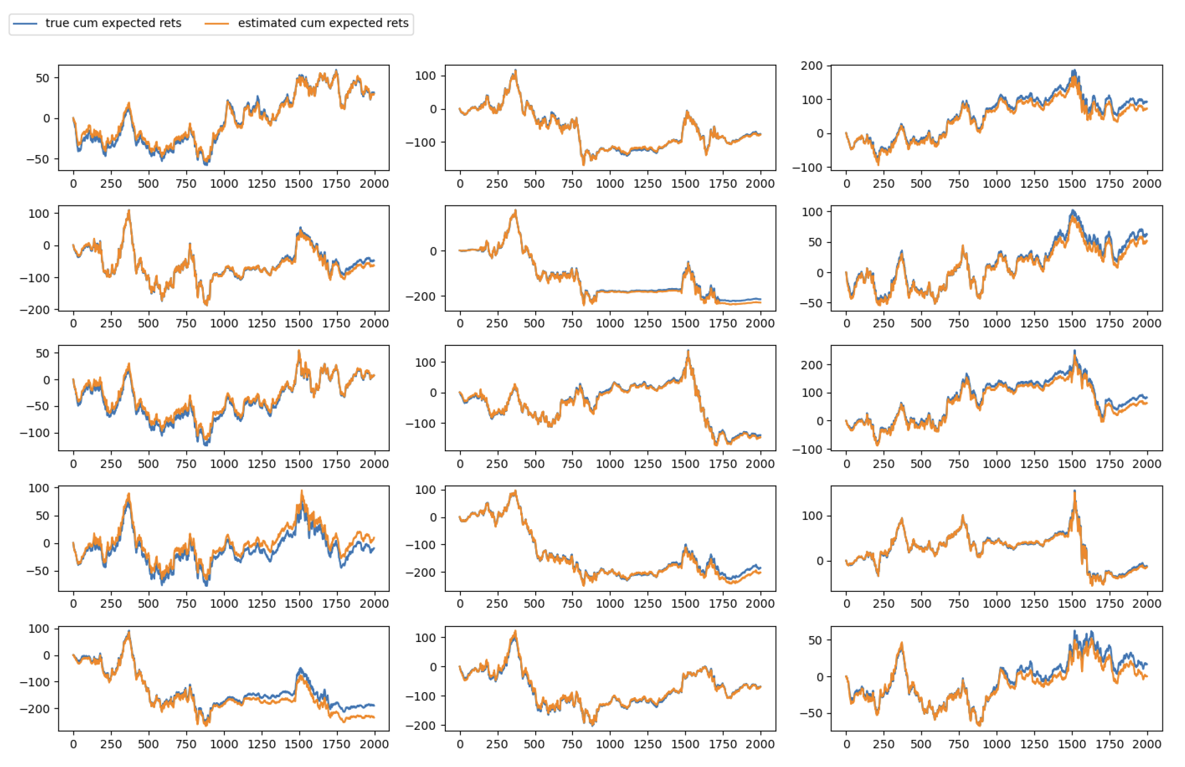
Since factor loadings and factor returns are not separately identifiable in our model structure, in this analysis, we mainly check regimes detection (See Figure 1), idiosyncratic risk estimation (See Figure 2), and cumulative expected returns’ tracking (See Figure 3). The estimation results are as follows:

Figure 1. Regime Detection.

Figure 1. Regime Detection.

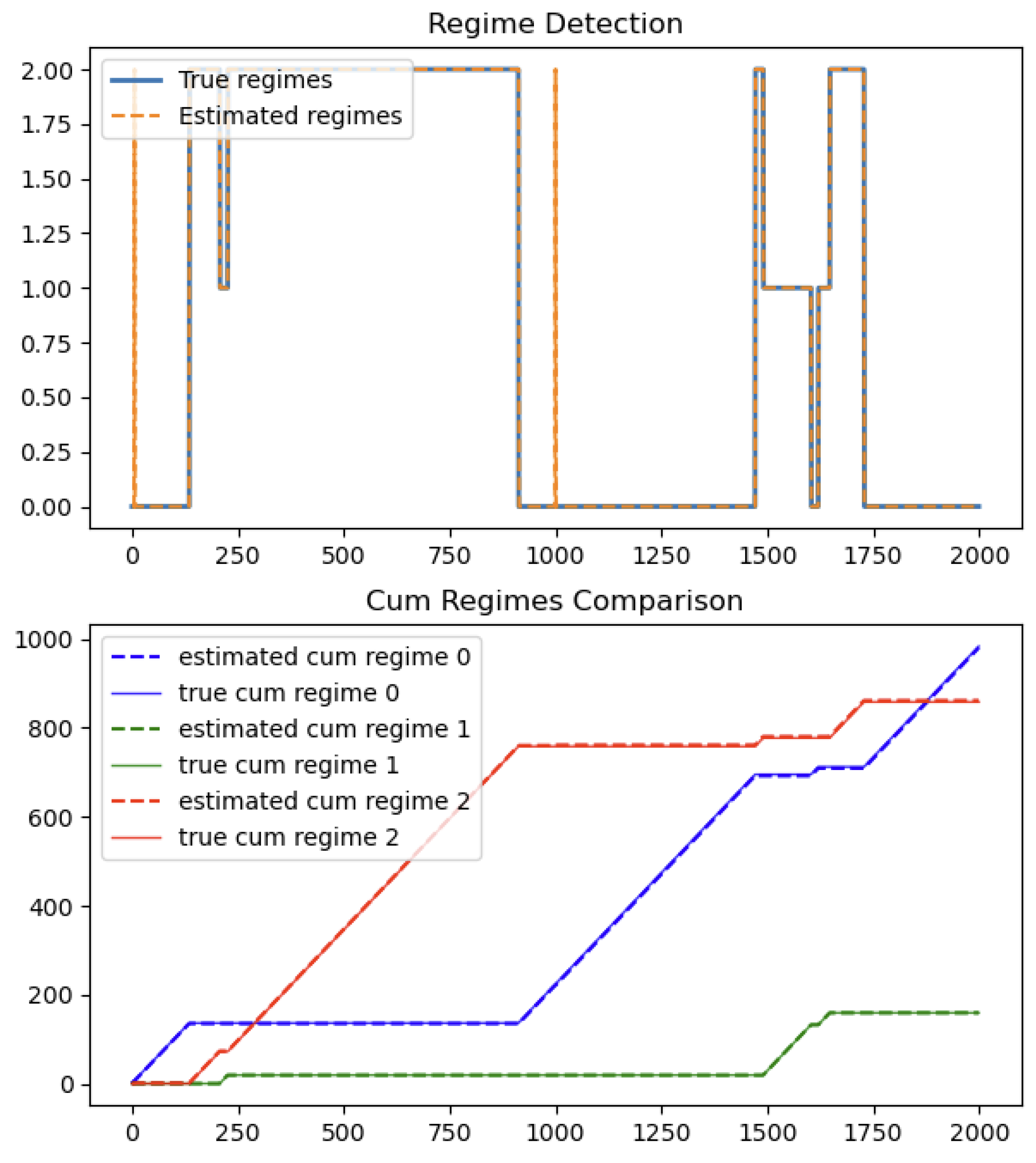
As shown in Figure 1, the algorithm accurately captures the evolution of hidden regimes from both regime detection plot and cumulative regimes comparison plot.

Figure 2. Idiosyncratic Risk Estimation.

Figure 2. Idiosyncratic Risk Estimation.

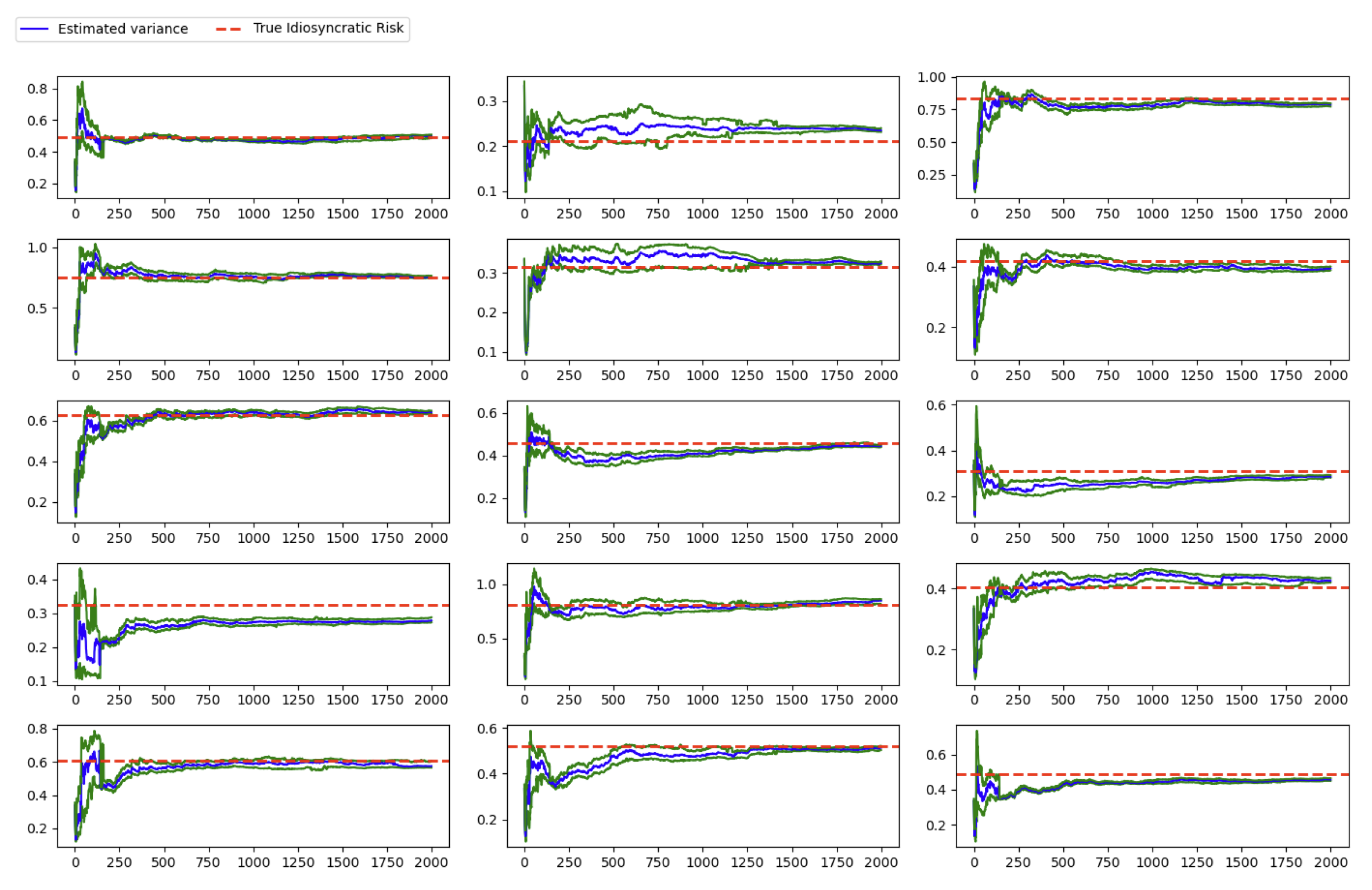
In terms if idiosyncratic risk (or error variance), the algorithm can also converge to their unbiased estimation.

The most important metric in statistical factor analysis is how accurately the model tracks the expected return. In this synthetic setting, our model demonstrates strong performance in the expected return (or cumulative expected return as shown in Figure 3) tracking.

Figure 3. Cumulative Expected Return Tracking.

Figure 3. Cumulative Expected Return Tracking.

4. Results in Statistical Arbitrage Strategy

In both academic and industry, equity statistical arbitrage strategy (equity stat-arb) usually means the idea of trading groups of stocks against either explicit or synthetic factors, which can be seen as the generalization of “pairs-trading” (see [29]). In some cases, we would long an individual stock and short the factors, and in others we would short the stock and long the factors. Overall, due to the netting of long and short positions, our exposure to the factors will be small. One key step of the equity stat-arb strategy is the decomposition of assets’ returns into the systematic part and idiosyncratic part. When we use a more effective factor model, we can have a better decomposition and hence the better strategy performance.

4.1. Market Neutral Strategy

In this paper, we evaluate the quality of factor models within the context of an equity statistical arbitrage strategy. Inspired by the approach of [30], in order to avoid the unnecessary complexity of signal generation and potential overfitting issues we adopt a deliberately simple reversion signal which is the negative value of previous day’s residuals. To ensure market neutrality, we construct a dollar-neutral portfolio each day, with equal dollar amounts allocated to long and short positions.

To be specific, we compare the performance of trading strategies derived from both regime switching dynamic factor model and static MLE factor model. For the regime switching dynamic factor model, the factor loading matrices for each regime are initialized using estimates from a mixture of factor analyzer (MFA), trained on a “burnin” data from 2005-01-03 to 2011-01-01. The residualization step is implemented in a rolling window framework so that the residuals are always generated out-of-sample.

After the residualization step, we can generate our signals using naive rule-based approach. If previous day’s residual for asset i has $v_{i,t-1}>d$, where d is the threshold, then we will say that the asset i is over-priced at time $t-1$ and short this asset for the next time stamp t. For $v_{i,t-1}<-d$, we will do the opposite operation. At each time step, we form a dollar-neutral portfolio with equally weighted positions on both the long and short sides.

4.2. Performance Comparison

We run this naive strategy using both dynamic factor model and static factor model respectively, and the strategy performance is given as Figure 4:

Figure 4. Equity Stat-Arb Performance Comparison.

Figure 4. Equity Stat-Arb Performance Comparison.

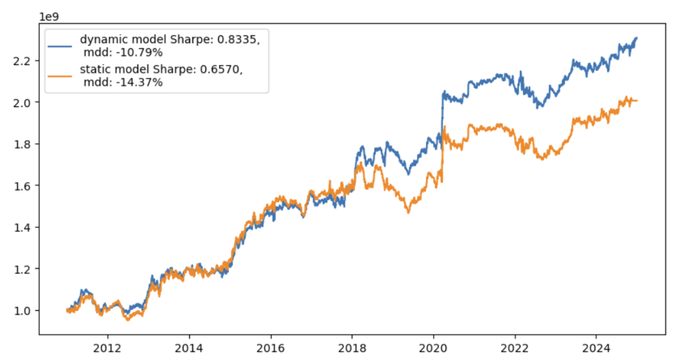
We can see from Figure 4 that the strategy has a better Sharpe and lower Maximum drawdown when using regime switching dynamic factor model than using static MLE factor model. The associated historical effective sample size plot and regime detection plot are given in Figure 5:

Figure 5. (a) Effective Sample Size at each day when running particle filter (a) Regime detection when using regime switching particle filter.

Figure 5. (a) Effective Sample Size at each day when running particle filter (a) Regime detection when using regime switching particle filter.

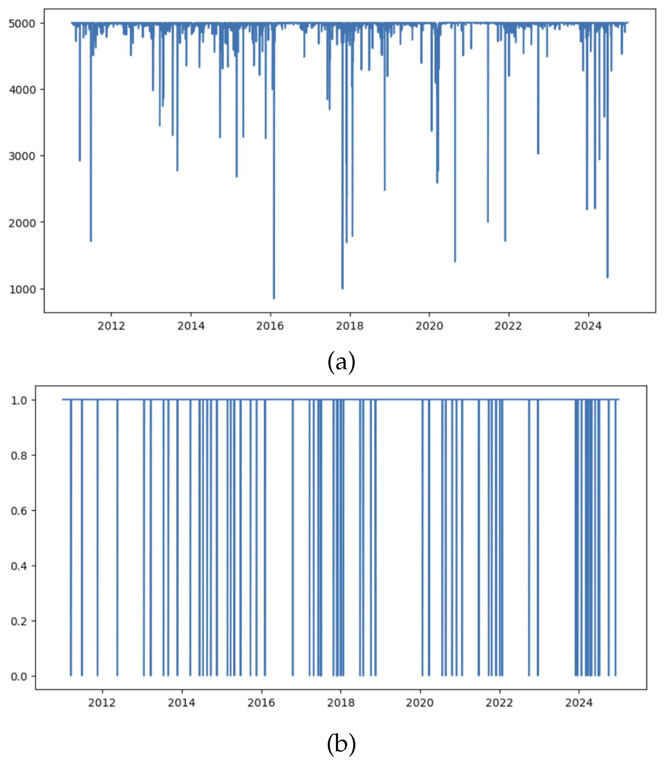
From the effective sample size, we can see the particle filter estimation is stable since most of the sample size are larger than 1000 for a three-factor model. From the regimes detection, we can see there are more regime changes in 2024 and indeed the strategy relying on regime switching dynamic factor model performs better in 2024 than the one using static model.

5. Discussion

This paper investigates the estimation of regime switching dynamic factor model using a particle learning algorithm. Through simulation studies, we validate our estimation approach by evaluating regime detection accuracy, idiosyncratic risk estimation, and the model’s ability to track expected returns. Empirical study in the equity statistical arbitrage framework further demonstrates that the regime-switching dynamic factor model outperforms a conventional static MLE factor model in capturing underlying data dynamics.

The particle learning algorithm implemented in this paper builds on the framework of [15], with several modifications. First, we extend the innovation distribution to a mixture of Gaussian distributions. Second, we simplify the parameter learning step by only tracking the sufficient statistics, rather than using the marginalization via simulation. Last, we apply the estimated model to the empirical data and compare its performance against the conventional MLE factor model.

We are able to see the performance improvements in the equity statistical arbitrage strategy when using our model. Our model not only improves the Sharpe ratio but also minimizes the maximum drawdown. These results align with our initial motivation: It is well known that financial market operates under multiple regimes, incorporating the regime switching mechanism that is governed by hidden Markov model in our model representation allows us better model the structural shifts and enhances risk management — particularly during periods of elevated volatility and contagion risk.

While the current particle learning algorithm is based on the vanilla auxiliary particle filter, there remains a lot of room to improve the quality of our particle filtering algorithm and hence improve the tracking of hidden states (or hidden factor in this model). For instance, the ABC-based sequential Monte Carlo filter [31] could further enhance the filtering accuracy. Additionally, incorporating more robust, heavy-tailed innovation distributions [32] may improve the robustness of our estimation, particularly in the presence of extreme market movements.

References

- Barra, M. Barra Risk Model Handbook; MSCI, 2004.
- Jolliffe, I.T. Principal component analysis, 2. ed., [nachdr.] ed.; Springer series in statistics; Springer: New York, 2004. [Google Scholar]
- Hinton, G.; Dayan, P.; Revow, M. Modeling the manifolds of images of handwritten digits. IEEE Transactions on Neural Networks 1997, 8, 65–74. [Google Scholar] [CrossRef]
- McLachlan, G.; Peel, D. Finite Mixture Models; Wiley, 2000. [CrossRef]
- Rubin, D.B.; Thayer, D.T. EM Algorithms for ML Factor Analysis. Psychometrika 1982, 47, 69–76. [Google Scholar] [CrossRef]
- Zoubin Ghahramani, G.E.H. Parameter Estimation for Linear Dynamical Systems. Technical Report CRG-TR-96-2, 1996. [Google Scholar]
- Bai, J.; Wang, P. Identification and Bayesian Estimation of Dynamic Factor Models. Journal of Business Economic Statistics 2014, 33, 221–240. [Google Scholar] [CrossRef]
- Kim, C.J.; Halbert, D.C.R. State-Space Models with Regime Switching: Classical and Gibbs-Sampling Approaches with Applications; The MIT Press, 1999. [CrossRef]
- Geweke, J.; Zhou, G. Measuring the price of the Arbitrage Pricing Theory. The Review of Financial Stuidies, vol. 9, no.2, 1996. [Google Scholar]
- Forni, Mario, D. G.M.L.; Reichlin, L. Opening the Black Box: Structure Factor Models with Large Cross Sections. Econometric Theory 25, no. 5 2009. [Google Scholar]
- Doucet, A.; Johansen, A.M. A tutorial on particle filtering and smoothing: Fifteen years later. Handbook of nonlinear filtering 2009. [Google Scholar]
- Arulampalam, M.; Maskell, S.; Gordon, N.; Clapp, T. A tutorial on particle filters for online nonlinear/non-Gaussian Bayesian tracking. IEEE Transactions on Signal Processing 2002, 50, 174–188. [Google Scholar] [CrossRef]
- Liu, J.; West, M. , Combined Parameter and State Estimation in Simulation-Based Filtering. In Sequential Monte Carlo Methods in Practice; Springer New York, 2001; pp. 197–223. [CrossRef]
- Djuric, P.M.; Khan, M.; Johnston, D.E. Particle Filtering of Stochastic Volatility Modeled With Leverage. IEEE Journal of Selected Topics in Signal Processing 2012, 6, 327–336. [Google Scholar] [CrossRef]
- Carvalho, C.M.; Johannes, M.S.; Lopes, H.F.; Polson, N.G. Particle Learning and Smoothing. Statistical Science 2010, 25. [Google Scholar] [CrossRef]
- Gordon, N.; Salmond, D.; Smith, A. Novel approach to nonlinear/non-Gaussian Bayesian state estimation. IEE Proceedings F Radar and Signal Processing 1993, 140, 107. [Google Scholar] [CrossRef]
- Doucet, A.; Godsill, S.; Andrieu, C. On sequential Monte Carlo sampling methods for Bayesian filtering. Statistics and Computing 2000, 10, 197–208. [Google Scholar] [CrossRef]
- Pitt, M.K.; Shephard, N. Filtering via Simulation: Auxiliary Particle Filters. Journal of the American Statistical Association 1999, 94, 590–599. [Google Scholar] [CrossRef]
- Kantas, N.; Doucet, A.; Singh, S.S.; Maciejowski, J.; Chopin, N. On Particle Methods for Parameter Estimation in State-Space Models. Statistical Science 2015, 30. [Google Scholar] [CrossRef]
- Schon, T.; Gustafsson, F.; Nordlund, P.J. Marginalized particle filters for mixed linear/nonlinear state-space models. IEEE Transactions on Signal Processing 2005, 53, 2279–2289. [Google Scholar] [CrossRef]
- Storvik, G. Particle filters for state-space models with the presence of unknown static parameters. IEEE Transactions on Signal Processing 2002, 50, 281–289. [Google Scholar] [CrossRef]
- Özkan, E.; Šmídl, V.; Saha, S.; Lundquist, C.; Gustafsson, F. Marginalized adaptive particle filtering for nonlinear models with unknown time-varying noise parameters. Automatica 2013, 49, 1566–1575. [Google Scholar] [CrossRef]
- Lopes, H.F.; Tsay, R.S. Particle filters and Bayesian inference in financial econometrics. Journal of Forecasting 2010, 30, 168–209. [Google Scholar] [CrossRef]
- CARTER, C.K.; KOHN, R. On Gibbs sampling for state space models. Biometrika 1994, 81, 541–553. [Google Scholar] [CrossRef]
- Andrieu, C.; Doucet, A.; Holenstein, R. Particle Markov Chain Monte Carlo Methods. Journal of the Royal Statistical Society Series B: Statistical Methodology 2010, 72, 269–342. [Google Scholar] [CrossRef]
- Del Moral, P. , Feynman-Kac Formulae. In Feynman-Kac Formulae; Springer New York, 2004; pp. 47–93. [CrossRef]
- Urteaga, I.; Bugallo, M.F.; Djurić, P.M. Sequential Monte Carlo for inference of latent ARMA time-series with innovations correlated in time. EURASIP Journal on Advances in Signal Processing 2017, 2017. [Google Scholar] [CrossRef]
- Carlin, B.P.; Polson, N.G. Inference for nonconjugate Bayesian Models using the Gibbs sampler. Canadian Journal of Statistics 1991, 19, 399–405. [Google Scholar] [CrossRef]
- Avellaneda, M.; Lee, J.H. Statistical arbitrage in the US equities market. Quantitative Finance 2010, 10, 761–782. [Google Scholar] [CrossRef]
- Khandani, A.E.; Lo, A.W. What Happened to the Quants in August 2007?: Evidence from Factors and Transactions Data. SSRN Electronic Journal 2008. [Google Scholar] [CrossRef]
- Jasra, A.; Singh, S.S.; Martin, J.S.; McCoy, E. Filtering via approximate Bayesian computation. Statistics and Computing 2010, 22, 1223–1237. [Google Scholar] [CrossRef]
- Schoutens, W. Lévy processes in finance, reprinted ed.; Wiley series in probability and statistics; Wiley: Chichester [u.a.], 2005. [Google Scholar]
- Murphy, K.P. Machine Learning - A Probabilistic Perspective; Adaptive Computation and Machine Learning, MIT Press: Cambridge, 2014; Description based upon print version of record. [Google Scholar]
Disclaimer/Publisher’s Note: The statements, opinions and data contained in all publications are solely those of the individual author(s) and contributor(s) and not of MDPI and/or the editor(s). MDPI and/or the editor(s) disclaim responsibility for any injury to people or property resulting from any ideas, methods, instructions or products referred to in the content. |
© 2025 by the authors. Licensee MDPI, Basel, Switzerland. This article is an open access article distributed under the terms and conditions of the Creative Commons Attribution (CC BY) license (https://creativecommons.org/licenses/by/4.0/).
Copyright: This open access article is published under a Creative Commons CC BY 4.0 license, which permit the free download, distribution, and reuse, provided that the author and preprint are cited in any reuse.