

Submitted:
22 July 2025
Posted:
24 July 2025
You are already at the latest version
Abstract
The impact of electricity consumption on financial development is a critical issue in the emerging market economies (EMEs), with no consensus amongst scholars and policy-makers on its impact on financial development. This paper investigates the long-term and causal relationship between electricity consumption and financial development using panel cointegration analysis and the error correction model for a panel of 20 se-lected EMEs from 2000 to 2020. The findings indicate a positive long-term cointegrating relationship between electricity consumption and financial development. There is a stable long-run equilibrium, as confirmed by the error correction term, with a deviation correction of 29% per period. The result of the study highlights the importance for EMEs to prioritise investments in energy infrastructure that will act as a catalyst for financial development. Furthermore, there is a need for policies that align electricity consumption with financial development goals. This ensures that there is sustainable energy access is a key ingredient in financial stability in emerging markets.
Keywords:
electricity consumption
; emerging market economies
; energy consumption
; financial development
1. Introduction
Financial development plays a crucial role in ensuring the efficient allocation of resources in an economy (Aman et al., 2023; Levine, 1997). The efficient allocation of resources creates a fertile ground for innovation through the allocation of resources to stimulate productivity in an economy (Wooldridge, 2020). Moreover, developed financial systems provide a buffer that allows the economies to withstand macroeconomic shocks (Aman et al., 2023). Furthermore, the development of financial systems is critical in attracting capital flows (Fang, Ouyang & Chen 2023; Alfaro, Kalemli-Ozcan & Volosovych 2008).
Financial markets in the EMEs have grown significantly since 1997 in terms of breadth and depth. However, the growth of the financial markets has not been proportional across the EMEs, and in general, they are behind the advanced economies that are more stable and developed. This disparity has created structural weaknesses, particularly in their capacity to fund capital-intensive energy projects (Wooldridge, 2020). The exogenous factors increase the vulnerability of the markets in the emerging markets. The COVID-19 outbreak in 2020 underscored this fragility, resulting in capital flight from EMEs to advanced economies (Wen, Mahmood, Khalid & Zakaria 2022). According to the International Monetary Fund (2023), investors are still exercising great caution, and they are biased towards markets with perceived resilience and stronger macroeconomic fundamentals. Resultantly, there have been improvements in at-risk capital flows in EMEs, indicating strong risk appetite in global markets.
Energy markets are constrained by challenges emanating from security concerns, emissions, and geopolitical instability. The COVID-19 pandemic and the Ukraine war negatively impacted global energy supply chains (International Energy Agency 2023). The dependence of global energy markets on major supplies like Russia was exposed as a result of the Russian/Ukraine war (World Bank 2022). Instability has been aided by inflationary pressures, constrained growth prospects, and volatile energy markets.
Most of the economies in the EMEs have unlocked their economies from the stifling lockdowns of 2020- 2021. As a result, there has been economic recovery, and electricity demand has been increasing gradually. EMEs are forecasted to drive energy demand with a projected increase of 3.4% between 2024 – 2026. This is likely to lead to an energy crisis compounded by high inflation, high interest rates, and debt that will exert pressure on the economies. According to Odhiambo (2023), the onboarding of 7.4 million households in South Africa to the main grid between 1994 and 2018 through the rural electrification programs. This took away the electricity margin since the increase in demand was not matched by a corresponding increase in supply. EMEs continue to lag behind the advanced economies in terms of energy investment, efficiency and transition.
Figure 1 indicates that electricity demand is expected to increase on the back of strong growth in emerging markets and industrial recovery. The emerging markets are expected to have an increase of 85%, with China being at the lead. The onboarding of the residential, transportation, and industrial sectors onto the main grid is going to exert more pressure on electricity demand. Cryptocurrencies and artificial intelligence (AI) are expected to double by 2026. The growth in AI and cryptocurrencies is expected to drive economic growth in EMEs by between 4% and 4.1% between 2024 and 2026. Resulting from this growth electricity consumption share within the overall energy consumption matrix is expected to increase by 2% to 20% from 18% in 2015 (IEA, 2024).
The current study is premised on the following hypotheses:
H1: Financial development has a significant effect on electricity consumption.
H2: Electricity Consumption has a significant effect on financial development.
There remains a dearth of literature that focuses on emerging market economies despite growing literature on the nexus between financial development and electricity consumption (Durusu-Ciftci, Soytas & Nazlioglu, 2020). The study of the relationship between two variables is important as economies transition from largely agro-based economies to more industrialized economies, leading to fundamental changes in the energy and financial markets. The emerging markets have a unique interaction between financial development and energy consumption as the economies are undergoing through transformation process (Durusu-Ciftci et al., 2020). The study investigates the relationship between financial development and electricity consumption in the EMEs using the cointegrating and causality tests for the period 2000 – 2020. The research provides important insights into energy policy and development in the context of EMEs. It also contributes to the literature by addressing the interplay between financial development and electricity consumption in these economies.
2. Literature Review
Financial development has three dimensions of depth, access, and efficiency. The deeper markets tend to be more liquid and have a lot more institutional investors' support, which provides a steady source of project financing (Bao Dinh & Tran, 2024; Catalan et al, 2000). As the financial sector becomes deeper, it becomes more resilient to credit and liquidity shocks (Rena & Kamuinjo, 2022; Impavido et al, 2002), and a developed market has more scope for macroeconomic risk diversification (Kapingura, Mkosana & Kusairi, 2022; Impavido & Tower, 2009). Advanced markets are deemed to have more depth, access, and efficiency as compared to less developed markets (Caucasus, 2022). As propounded by Levine (1997) and King & Levine (1993), financial development is critical in savings mobilisation and allocation of the same to the productive sector. This supports output and growth of the economies, and financial development is a good predictor of future growth. Countries must achieve growth; they must have strong support structures that propagate financial innovation and growth. Lack of innovation is viewed as a reason that stifles growth in developing countries, see for example (Bozkurt, 2022).
There are two categories of financial development indicators: The first category includes quantitative and structural measures, such as financial prices, product range, and transaction costs (Bozkurt, 2022). The second category includes market-based and institutional indicators encompassing the size of the financial institutions and markets (financial depth), market access, financial institutions' efficiency (FIE), and markets' robustness (reliability) (Sahay et al., 2015). These two categories consider money demand variables like the M1, M2, M2Y, M3, interest rates, total financial sector assets, and the number of people with bank accounts (Levine, 2004).
Building on this classification, this study used the framework as developed by Sahay et al. (2015), which covered 183 advanced economies, emerging markets, and low-income countries. Using principal component analysis, they constructed a multi-dimensional financial development index, capturing the performance of financial institutions and markets across three key dimensions: depth, access, and efficiency. The framework is synthesised into nine indices: the overarching Financial Development Index, two sub-indices—Financial Institutions Index and Financial Markets Index—and further subdivisions within each. The Financial Institutions Index is broken down into depth, access, and efficiency, while the Financial Markets Index consists of financial market depth, access, and efficiency. In this study, the primary focus is on the Financial Development Index, along with the Financial Institutions Index and the Financial Markets Index as sub-components, as indicated in Figure 2.
2.1. Theoretical Literature Review
There has been extensive research on the relationship between financial development and electricity consumption in the context of emerging market economies (EMEs). This relationship is particularly important as the emerging market economies (EMEs) undergo rapid industrialisation and urbanisation. Electricity consumption plays a critical role in the sustenance and propagation of economic activities and productivity enhancement (see Durusu-Ciftci, Soytas & Nazlioglu, 2020; Sadorsky, 2010).
However, despite these extensive studies on the nexus, there is no consensus among researchers. Four positions are propagated regarding the relationship between electricity consumption and financial development, these include: The Financial Development led Energy Demand Hypothesis, the energy-led financial development hypothesis, the bidirectional causality hypothesis, and the neutrality hypothesis (Odhiambo, 2023; Nyasha & Odhiambo, 2018):
2.1.1. Financial Development Led Energy Demand Hypothesis
This hypothesis postulates that financial development is the key driver of electricity consumption (Ma & Fu, 2020; Sadorsky, 2010). In developed financial markets, it is easier to finance energy-intensive purchases and investments at both personal and corporate levels, which inevitably increases energy consumption (Zaidi, Zafar, Shahbaz & Hou 2019). This view is in line with the supply-leading hypothesis, which posits that financial development stimulates economic activities, leading to increased energy demand (King & Levine, 1993).
2.1.2. The Energy-Led Financial Development Hypothesis
This argument posits that energy consumption has a positive impact on financial development. This emanates from the fact that as electricity consumption increases, financial transactions and investments inevitably increase (Odhiambo, 2023; Karanfil, 2009). Furthermore, as industrial activities increase, demand for financial services increases, hence resulting in the deepening of financial markets (Shahbaz, Hoang, Mahalik & Roubaud, 2017).
2.1.3. The Bidirectional Causality Hypothesis
This argues for the existence of a cyclical process between electricity consumption and financial development. The findings of (Ma, Zhao, Jia, Wang & Zhang 2022; Islam, Shahbaz, Ahmed & Alam 2013) support the notion that the development of financial markets results in efficient allocation of capital into energy markets, which in turn supports economic growth and further financial development. This mutual causality aligns with the endogenous growth theory, which posits that financial and energy sectors jointly contribute to sustained long-term economic growth (Bencivenga & Smith, 1991).
2.1.4. The Neutrality Hypothesis
This hypothesis argues that there is no relationship between electricity consumption and financial development (Apergis & Tang, 2013; Narayan & Narayan, 2013). This is true in economies with underdeveloped financial markets or where energy markets are constrained, hence impeding industrial activity. This results in cases where energy markets evolve without the influence of the financial markets.
2.2. Empirical Literature Review
The relationship between electricity consumption and financial development is a key area of empirical research in EMEs. Energy demand has been increasing as a result of industrialisation and urbanisation. This has raised the need to have a deeper understanding of how financial markets influence electricity consumption. The causal relationship between these variables has been explored using advanced econometric techniques to establish the long-term and short-term linkages.
The study of (Chang 2014 and Islam et al. 2013) found that financial development results in the channelling of funds into energy-intensive industries and infrastructure, increasing electricity demand. Furthermore, the studies of (Lefatsa, Sibanda & Garidzirai, 2021; Ma & Fu, 2020) emphasise that easy access to credit allows consumers to afford electricity-consuming products, hence increasing energy consumption. These findings are premised on the notion that developed financial markets drive electricity consumption through credit availability and facilitation of investment.
This is contrasted with other studies that found that electricity consumption instigates financial development, through the energy-led financial development hypothesis. According to Karanfil (2009), increased electricity demand results in increased business activity, leading to increased demand for financial services. Odhiambo (2023) further argues that increased electricity demand results in economic growth, hence increasing credit demand and investment opportunities.
A bidirectional relationship between financial development and electricity consumption has been identified in empirical studies. The findings of (Ma et al., 2022; Sahay et al., 2015; Islam, Shahbaz, Ahmed, Alam, et al., 2013) found that financial development and electricity consumption reinforce each other through the economic growth channel. These studies used the panel cointegration techniques and Granger causality tests. This bidirectional causality suggests that policies promoting financial sector deepening should consider energy sector improvements and vice versa to ensure sustainable growth.
Other studies argue that there is no relationship between financial development and electricity consumption, backed by the neutrality hypothesis, for example, the studies of (Caucasus, 2022; Tamazian, Chousa & Vadlamannati 2009). These studies' findings reinforce the notion that owing to structural differences in economic composition and regulatory frameworks, the energy and financial markets operate independently. These findings reinforce the fact that financial markets can develop and not resulting in increased electricity consumption. Some of the factors at play in the EMEs are the fact that they have low industrialisation levels.
Table 1 below presents summarised empirical findings of previous studies.
3. Data and Methodology
3.1. Data and Variables
The study used the data from the World Bank’s Global Financial Development Database and the Energy Information Administration as the primary and only sources of data. The study sampled 20 emerging market economies covering the period from 2000 to 2020. These countries were from Asia, Africa, Eastern Europe, Europe, North America, and South America. The specific countries are Argentina, Brazil, Chile, Colombia (South America), China, India, Indonesia, Iran, Malaysia, Philippines, Thailand, United Arab Emirites (Asia), Egypt, Kenya, Nigeria, Saudi Arabia, South Africa (Africa); Hungary, Russia, Turkey (Europe, Eastern Europe); Mexico (North America). This sample is diverse as it covers emerging economies from various continents and captures diverse geopolitical dynamics involved. The study used various econometric models on the sample.
The study looked at the following variables: energy consumption as proxied by electricity consumption from the Energy Information Administration. Financial development as proxied by financial development index, with the following control variables economic growth as proxied real GDP per capita, FDI, government effectiveness, infrastructure proxied by the gross fixed capital formation (GFCF % of GDP), inflation, real interest rates and resources sourced from the World Bank’s Global Financial Development Database. Table 2 gives a summary of the variables, definitions, and data sources.
Panel Unit Root Test
The study employed four main panel unit root tests performed in Stata (LLC, IPS, ADF-Fisher chi-square, and PP-Fisher chi-square), which originate from the time series unit root testing presented in Table 2. The panel unit root tests are performed for the diagnostic tests to establish the stationarity of the series. The individual unit root tests have no power in panel data sets, and this is worsened by small samples (Baltagi, 2008; Hsiao, 2014); hence, the standard unit root tests cannot be applied to this study.

Table 3.
1 Panel Unit Root Test using LLC.
| Variable | No trend | Intercept and Trend |
Individual Effects | Decision |
|---|---|---|---|---|
| EconGR1 | -9.00243*** | -14.1579*** | -14.8932*** | I(1) |
| ED1 | -5.19401*** | -3.51018*** | -3.39410*** | I(1) |
| FDI | -3.73481*** | -3.84931*** | -3.59057*** | I(1) |
| FIN_DEV1 | -12.5368*** | -5.76010*** | -7.01951*** | I(1) |
| GE | -19.2898*** | -11.6725*** | -5.32626*** | I(1) |
| GFCF | -3.17697*** | -4.81640*** | -12.7641*** | I(1) |
| INF | -5.36244*** | -3.17697*** | -4.81640*** | I(1) |
| INT | -4.55824*** | -2.94927*** | -2.98998*** | I(1) |
| RES | -17.1758*** | -11.7095*** | -12.5584*** | I(1) |
Table 4.
Panel unit root tests using IPS.
| Variable | No trend | Intercept and Trend |
Individual Effects | Decision |
|---|---|---|---|---|
| EconGR1 | - | -7.32238*** | -8.86368*** | I(1) |
| ED1 | - | -4.90339 | -6.80038*** | I(1) |
| FDI | - | -3.15388*** | -4.64037*** | I(1) |
| FIN_DEV1 | - | -6.80194*** | -8.89608*** | I(1) |
| GE | - | -7.76492*** | -3.37902*** | I(1) |
| GFCF | - | -5.22146*** | -6.27994*** | I(1) |
| INF | - | -4.60067*** | -4.43623*** | I(1) |
| INT | - | -3.99142*** | -5.53141*** | I(1) |
| RES | - | -8.61635 | -10.5161*** |
Table 5.
Panel unit root testing using ADF – Fisher Chi-square.
| Variable | No trend | Intercept and Trend |
Individual Effects | Decision |
|---|---|---|---|---|
| EconGR1 | 162.126*** | 119.625*** | 165.202*** | I(1) |
| ED1 | 97.4080*** | 97.5214** | 121.693*** | I(1) |
| FDI | 58.5960*** | 69.1745*** | 95.5074*** | I(1) |
| FIN_DEV1 | 205.413** | 121.031*** | 155.718*** | I(1) |
| GE | 298.930 | 137.193*** | 96.8117*** | I(1) |
| GFCF | 206.139*** | 101.597*** | 113.461*** | I(1) |
| INF | 78.4077*** | 89.8547*** | 89.4916*** | I(1) |
| INT | 111.210*** | 81.3262*** | 103.028*** | I(1) |
| RES | 293.299*** | 142.441*** | 180.638*** | I(1) |
Table 6.
Panel unit root testing using PP - Fisher Chi-square.
| Variable | No trend | Intercept and Trend |
Individual Effects | Decision |
|---|---|---|---|---|
| EconGR1 | 288.937*** | 183.140*** | 211.156*** | I(1) |
| ED1 | 196.560*** | 227.986*** | 279.949*** | I(1) |
| FDI | 62.4167*** | 99.6138*** | 125.058*** | I(1) |
| FIN_DEV1 | 342.526*** | 282.882*** | 338.690*** | I(1) |
| GE | 425.816*** | 119.393*** | 100.232*** | I(1) |
| GFCF | 282.949 | 168.619*** | 188.621*** | I(1) |
| INF | 125.836*** | 257.273*** | 195.883*** | I(1) |
| INT | 154.617*** | 172.350*** | 339.354*** | I(1) |
| RES | 384.238*** | 298.422*** | 293.773*** | I(1) |
***; **; * indicates that the null hypothesis of unit root tests is rejected at 1%, 5% and 10%, respectively. All the tests are at first difference (except where indicated otherwise). Probabilities for all the tests assume asymptotic normality except for Fisher tests which are computed using the asymptotic Chi-square distribution. ED1 is the Electricity Consumption, ED2 is the electricity generation, ED3 is the energy consumption per capita, ED4 is total energy consumption per GDP, ED5 is the total energy production, ED6 is the petroleum and other liquids, FIN_Dev1 is the financial development index, FIN_Dev2 is the financial institutions index, FD_Dev3 is the financial market index, EconGR1 is the Gross Domestic Product per capita, FDI is the foreign direct investment, GFCF is the Gross Fixed Capital Formation as % of GDP, INF is inflation, GE is the government effectiveness, INT is the real interest rates and RES is the total natural resources.
Source: Author’s compilation using Stata
The variables are integrated of order one, I(1), in all four testing methodologies. This indicates that variables exhibit non-stationarity in levels but become stationary after first differencing, justifying the need for panel cointegration analysis to determine long-run equilibrium relationships (Nkalu, Ugwu, Asogwa, Kuma & Onyeke 2020). The findings support further econometric modelling, such as panel VECM or ARDL, to assess dynamic interactions between financial development and electricity consumption in emerging markets (Bozkurt, Toktaş & Altiner 2022).
Descriptive Statistics
Table 7 provides the descriptive statistics of the study sample, covering emerging markets. The summary is inclusive of key macroeconomic variables relevant to the study.
Table 7 (above) and Table 8 (below) present the descriptive statistics and correlations, respectively, for the variables under investigation. FinDev1 represents financial development, ED1 represents electricity consumption, EconGR1 represents economic growth, FDI represents foreign direct investment, GE represents government effectiveness, GFCF represents gross fixed capital formation, INF represents inflation, INT represents real interest, and RES represents resources. The variables are weakly correlated, hence there is a minimum problem of multicollinearity. Cross-sectional dependence was tested for the model with an insignificant Pesaran’s (2021) CD test, implying that the cross-sections were independent.
The descriptive statistic summary in Table 7 can be summed up as follows: The financial development index (Fin_Dev1) ranged from 0.09 to 0.74, explaining the disparities in financial development maturity in different countries. The low mean score of 0.42 and a high standard deviation of 0.14 indicate that many countries have underdeveloped financial systems. This can be attributed to weak financial institutions, limited capital market depth, or regulatory inefficiencies in emerging markets. Electricity consumption (ED1) varied widely, ranging from 3.38 billion kWh to 7,115.08 billion kWh per capita. The mean electricity consumption was 385.61 billion kWh, and a high standard deviation of 934.45 billion kWh indicated wide disparities across EME countries. The wide variation is indicative that electricity access varies widely in different emerging market economies. These variations can be explained by varied levels of industrialisation, electrification rate, energy infrastructure, and policy frameworks.
GDP per capita (EconGR1), measured in constant 2015 US dollars, with a mean of $8,264.37 and a standard deviation of $9,618.28. The findings indicate economic heterogeneity within the sample. There was huge volatility in FDI volatility in FDI inflows among the EMEs. This is indicated by the mean of 3.08% of GDP and a huge standard deviation of 7.81. The gross fixed capital formation (GFCF) mean was 22.96% of GDP. This is suggestive of variations in capital accumulation patterns across countries.
Inflation ranged from -16.27% to 52.98%, with real interest rates ranging from -18.85% and 54.00%. The natural resource rents (RES) had a mean of 9.42% of GDP and a maximum of 55.48%.
Cross-Correlation Analysis
Table 8 reports the correlation coefficients, which measure the strength of the relationship between the variables in the variables.
There is a statistically significant but moderate positive correlation of 0.2947 between financial development (FIN_DEV1) and electricity consumption (ED1) at a 1% significance level. Among the control variables, there is a weak negative relationship of (-0.2951) between financial development (FIN_DEV1) and economic growth (ECONGR1). The weak positive correlation of FDI and financial development (0,0977**) indicates capital inflows facilitated by financial market depth, albeit to a limited extent. Government effectiveness (GE) indicates a strong positive correlation with financial development (0.5704) at the 1% level. Gross fixed capital formation (GFCF) is positively related to electricity consumption (0.6141***) and financial development (0.1923***), indicating the importance of investments in both sectors.
The macroeconomic stability indicators have mixed results: Inflation (INF) is significantly negatively related correlated with financial development (-0.2817***). On the other hand, real interest rates (INT) have a weak positive relationship (0.1063**). Natural resources rents and financial development had a negative correlation of (-0.0966**).
3.2. Empirical Analysis
The autoregressive distributed lag (ARDL) bounds testing approach was used in the study as propagated by (Nguyen, Bui, Vo & McAleer, 2019; Pesaran, Shin & Smith, 2001) to investigate the long-term cointegrated relationship between electricity consumption and financial development. The panel ARDL model is most suited where both N and T exceed 1, rather than a standard ARDL, which is typically applied to a single time series (Pesaran et al., 2001). Pesaran, Shin & Smith (1999) posit that the method allows estimation of long-run relationships between dependent and independent variables, even when the regressors are integrated at different levels, provided they are not I(2).
According to Narayan (2004), the panel ARDL framework is flexible as it can estimate both short and long-run dynamics within the same model, especially for small sample sizes. Furthermore, it can take into consideration both immediate and equilibrium relationships over time (Pesaran et al., 2001). The Akaike Information Criterion (AIC) and Bayesian Information Criterion (BIC). Schwarz Bayesian Criterion (SBC) guided the appropriate lag length selection in Stata, with the lowest values determining the optimal lag structure.
Hausman's (1978) test was conducted to determine the most suitable estimator among Pooled Mean Group (PMG), Mean Group (MG), or Dynamic Fixed Effects (DFE), as well as to assess the homogeneity of long-run coefficients across sections. When dealing with smaller panel datasets, the PMG estimator is preferred, as argued by (Pesaran et al., 1999). Furthermore, the PMG can combine features of the MG estimator. On the other hand, the major difference between PMG and MG estimators is in the ability to embrace both the features of the MG estimator while averaging the results across cross-sections for greater consistency (Pesaran et al., 1999). The PMG estimator assumes heterogeneity in short-run coefficients, intercepts, and error variances, while maintaining homogeneous long-run slope coefficients across cross-sections (Loayza & Ranciere, 2006).
The equation below is estimated to examine the relationship between electricity consumption and financial development in the selected emerging markets. The study ran the ARDL and error correction model (ECM) to capture the speed of adjustment when there is disequilibrium (Pesaran et al., 1999). This allows the capturing of both the cointegrating and the short-run effects of the variables under study (Wehncke, Marozva & Makoni, 2023; Nxumalo & Makoni, 2021; Makoni & Marozva, 2018; Engle & Granger, 1987). The following Error Correction Model (ECM) for financial development was tested empirically:
where:
- =The change in Financial Development for country i at time t.
- = The error correction term, which captures the long-run equilibrium relationship between financial development (FINDev), energy development (EDev), and economic growth (EG). The term represents the speed of adjustment back to equilibrium.
- = The lagged changes in financial development, accounting for short-term dynamics.
- = The short-run effects of changes in energy development and economic growth, respectively.
- = The country-specific fixed effect.
- = The error term or disturbance.
PMG Estimation
Table 9 presents a summarised Pooled Mean Group on the cointegrating and causality relationship between financial development, Fin_Dev1 (Financial Development Index), (ED1) electricity consumption and economic growth.
4. Discussion
The study provides empirical evidence on the relationship between financial development and electricity consumption, with economic growth and FDI as the control variables in the EMEs, through the panel cointegration analysis and error correction model (ECM). The findings are summarized as follows:
ECT: The error correction term (ECT) confirms cointegration and existence of a stable long term relationship between the variables. The ECT for electricity consumption model is -0.299 and -0.0538 respectively. This implies that 29.9% of deviations from the financial development equilibrium and 5.38% from the electricity consumption equilibrium are corrected per period, aligning to the initial findings of (Shahbaz & Lean, 2012; Adom, 2021; Nkalu et al., 2020).
Long-Run Relationships:
The long run coefficients in the study indicate the effect of the dependent variables (D.Fin_Dev1, D.ED1, D.EconGR1, D.FDI) are influenced by the dependent variables. This is shown by the models in each columns.
Electricity consumption (ED1) on Financial Development (Fin_Dev1): The model had positive and significant of 0.251*** coefficient. A unit increase in electricity consumption leads to 2.51% increase in financial development. This is indicative that electricity access deepens financial markets in EMEs. Energy markets plays a key role in the deepening of financial markets, banking penetration and capital accumulation, in line with empirical findings by Sadorsky (2012) and Shahbaz et al. (2016), Sbia et al., (2014).
Financial Development (Fin_Dev1) on Electricity Consumption (ED1): Financial development has a positive insignificant effect on electricity consumption with a (coefficient of 0.0428, p > 0.05, t = 1.80). While financial development is critical for energy infrastructure investment it does not have a robust impact in the long run.
Economic growth (EconGR1) on Electricity consumption (ED1): Economic growth has a significant impact on financial development (Fin_Dev1) with a significantly positive coefficient of (1.325***). Economic growth leads to output and consumption increase, hence driving electricity consumption.
FDI significantly influences electricity consumption but has no significant effect on financial development or economic growth. The FDI model shows weaker long-run relationships, with no significant coefficients for the explanatory variables.
Short-Run Relationships:
Electricity Consumption (D.ED1) on Financial Development (D.Fin_Dev1): The short relationship between electricity consumption negatively impact financial development in the short run. This differs with the long run findings, as in the short run electricity consumption negatively affect financial development. This can be caused by the diversion of resources from the financial sector (Sadorsky, 2010).
Financial Development (Fin_Dev1) on Electricity Consumption (D.ED1): The effect is negative and insignificant (coefficient = -0.00642, p > 0.05, t = -0.21), indicating no robust short-run impact.
Results
Causality Implications:
- All the models had negative and significant ECTs indicating bidirectional causality in the long run. It indicates that deviations are corrected over time.
- Policies that strengthen energy access and security are key in supporting financial development and economic growth (Komal & Abbas, 2015).
- In the short run there are potential trade offs between between electricity consumption and financial development. This can be explained by diversion of resources from financial sector development in the short run.
- FDI’s significant positive effect on electricity consumption highlights the role of foreign investment in driving energy demand, likely through industrial or infrastructure projects.
5. Conclusions
This study contributes to the ongoing discourse on the electricity–finance nexus by providing robust empirical evidence from 20 emerging market economies (EMEs) over the period 2000–2020. Using panel cointegration and error correction techniques, the analysis reveals a significant long-term positive relationship between electricity consumption and financial development. The presence of a stable equilibrium relationship, albeit with a moderate speed of adjustment at 29% per period, underscores the critical role of energy infrastructure in driving financial sector growth in EMEs.
6. Patents
Funding
This research received no external funding.
Conflicts of Interest
The authors declare no conflicts of interest.
Abbreviations
The following abbreviations are used in this manuscript:
| ADF | Augmented Dickey-Fuller |
| AIC | Akaike Information Criterion |
| ARDL | Autoregressive Distributed Lag |
| BIC | Bayesian Information Criterion |
| CC BY | Creative Commons Attribution |
| CD | Cross-sectional Dependence |
| DFE | Dynamic Fixed Effects |
| ECM | Error Correction Model |
| ED1 | Electricity Consumption |
| ED2 | Electricity Generation |
| ED3 | Energy Consumption per Capita |
| ED4 | Total Energy Consumption per GDP |
| ED5 | Total Energy Production |
| ED6 | Petroleum and Other Liquids |
| EconGR1 | Gross Domestic Product per Capita |
| EMEs | Emerging Market Economies |
| FDI | Foreign Direct Investment |
| FIE | Financial Institutions' Efficiency |
| Fin_Dev1 | Financial Development Index |
| Fin_Dev2 | Financial Institutions Index |
| Fin_Dev3 | Financial Markets Index |
| GFCF | Gross Fixed Capital Formation |
| GE | Government Effectiveness |
| IEA | International Energy Agency |
| INF | Inflation |
| INT | Real Interest Rates |
| IPS | Im-Pesaran-Shin |
| LLC | Levin-Lin-Chu |
| MG | Mean Group |
| PMG | Pooled Mean Group |
| PP | Phillips-Perron |
| RES | Total Natural Resources Rents |
| SBC | Schwarz Bayesian Criterion |
| Sys-GMM | System Generalized Method of Moments |
| VECM | Vector Error Correction Model |
Appendix A
Appendix A.1: Causal and cointegrating relationships -Fin_Dev1
| PMG | MG | DFE | |
| D.Fin_Dev1 | D.Fin_Dev1 | D.Fin_Dev1 | |
| Long-Run | |||
| EconGR1 | -0.0143** | -0.163* | 0.0129 |
| (-3.27) | (-1.96) | (1.40) | |
| ED1 | 0.251*** | 0.694** | 0.266*** |
| (11.34) | (3.17) | (5.69) | |
| FDI | 0.00109 | 0.00658 | 0.00169 |
| (1.06) | (1.51) | (1.43) | |
| ECT | -0.299*** | -0.559*** | -0.215*** |
| (-5.33) | (-8.61) | (-7.09) | |
| Short-Run | |||
| D.EconGR1 | 0.0226 | 0.0877* | -0.00439 |
| (1.04) | (2.22) | (-1.08) | |
| D.ED1 | -0.249* | -0.325*** | -0.0197 |
| (-2.45) | (-3.95) | (-0.33) | |
| D.FDI | 0.000450 | -0.00112 | -0.000232 |
| (0.34) | (-0.77) | (-1.03) | |
| _cons | 0.00570 | -0.0218 | -0.0422 |
| (0.47) | (-0.15) | (-1.66) | |
| N | 399 | 399 | 399 |
Appendix A.2: Causal and cointegrating relationships -EconGr1
| PMG | MG | DFE | |
| D.EconGR1 | D.EconGR1 | D.EconGR1 | |
| ECT | |||
| Fin_Dev1 | 2.422 | 5.084 | 0.487 |
| (1.65) | (0.69) | (0.18) | |
| ED1 | 1.596*** | -0.115 | -0.410 |
| (4.59) | (-0.05) | (-0.35) | |
| FDI | 0.0120 | 0.159 | 0.0203 |
| (0.95) | (0.99) | (0.92) | |
| SR | |||
| ECT | -0.125*** | -0.423*** | -0.143*** |
| (-3.80) | (-10.70) | (-6.01) | |
| D.Fin_Dev1 | -0.896 | -1.157 | -0.317 |
| (-0.83) | (-0.76) | (-0.51) | |
| D.ED1 | 0.664 | 1.296 | -0.296 |
| (0.67) | (1.11) | (-0.40) | |
| D.FDI | 0.0123 | 0.000636 | -0.00254 |
| (0.71) | (0.03) | (-0.91) | |
| _cons | 0.0990 | 1.470 | 0.879** |
| (1.23) | (0.88) | (2.82) | |
| N | 399 | 399 | 399 |
t statistics in parentheses, * p < 0.05, ** p < 0.01, *** p < 0.001.
Appendix A.3: Causal and cointegrating relationships -ED1
| PMG | MG | DFE | |
| D.ED1 | D.ED1 | D.ED1 | |
| ECT | |||
| Fin_Dev1 | 1.325*** | -1.195 | 0.605 |
| (9.88) | (-0.49) | (1.51) | |
| EconGR1 | 0.0428 | 0.293 | -0.00245 |
| (1.80) | (1.86) | (-0.08) | |
| FDI | 0.0394*** | -0.0169 | -0.0000985 |
| (3.97) | (-1.18) | (-0.03) | |
| SR | |||
| ECT | -0.0538*** | -0.193*** | -0.0578*** |
| (-3.29) | (-4.22) | (-5.23) | |
| D.Fin_Dev1 | -0.0573 | -0.118 | -0.00825 |
| (-1.19) | (-1.39) | (-0.19) | |
| D.EconGR1 | -0.00642 | -0.0604 | -0.00151 |
| (-0.21) | (-1.45) | (-0.44) | |
| D.FDI | -0.00255 | -0.000947 | 0.0000484 |
| (-1.30) | (-0.57) | (0.25) | |
| _cons | 0.0783*** | 0.0779 | 0.126*** |
| (3.69) | (0.51) | (6.13) | |
| N | 399 | 399 | 399 |
t statistics in parentheses, * p < 0.05, ** p < 0.01, *** p < 0.001.
Appendix A.4: Causal and cointegrating relationships -FDI
| PMG | MG | DFE | |
| D.FDI | D.FDI | D.FDI | |
| ECT | |||
| Fin_Dev1 | -3.231 | 13.86 | -5.132 |
| (-1.56) | (1.69) | (-0.37) | |
| EconGR1 | -0.0459 | 4.792 | 0.283 |
| (-0.40) | (1.47) | (0.33) | |
| ED1 | 0.846 | 40.34 | 2.386 |
| (1.04) | (0.85) | (0.41) | |
| SR | |||
| ECT | -0.589*** | -0.842*** | -0.700*** |
| (-8.57) | (-11.45) | (-10.67) | |
| D.Fin_Dev1 | 12.18 | -0.872 | 15.24 |
| (1.12) | (-0.22) | (1.01) | |
| D.EconGR1 | -0.226 | -1.929 | 0.0108 |
| (-0.14) | (-1.26) | (0.01) | |
| D.ED1 | 3.677 | -7.589 | 3.628 |
| (0.53) | (-0.42) | (0.21) | |
| _cons | 1.775* | -63.98 | -1.015 |
| (2.49) | (-1.11) | (-0.13) | |
| N | 399 | 399 | 399 |
References
- Aman, A. , Khan, M. A., Khan, M. A., Haider, A., Oláh, J., & Fenyves, V. Role of institutions in promoting finance in emerging markets: A panel data analysis. PLOS ONE 2023, 18, e0280849. [Google Scholar] [CrossRef]
- Levine, R. Financial development. Financial Development and Economic Growth: Views and Agenda 1997, 2, 338–354. [Google Scholar] [CrossRef]
- Wooldridge, P. (2020). Implications of financial market development for financial stability in emerging market economies. Bank for International Settlements. https://www.bis.org/publ/othp32.
- Fang, L. , Ouyang, S., & Chen, V. (2023). International capital flows, financial development and economic growth fluctuations. In CCPF Conference (pp. 1–35).
- Alfaro, L. , Kalemli-Ozcan, S. , & Volosovych, V. Why doesn’t capital flow from rich to poor countries? An empirical investigation. Review of Economics and Statistics 2008, 90, 347–368. [Google Scholar] [CrossRef]
- Wen, J. , Mahmood, H. , Khalid, S., & Zakaria, M. The impact of financial development on economic indicators: A dynamic panel data analysis. Economic Research-Ekonomska Istraživanja 2022, 35, 2930–2942. [Google Scholar] [CrossRef]
- International Monetary Fund. (2023). Global financial stability report: Financial and climate policies for a high-interest-rate era. https://www.imf. 2023.
- International Energy Agency. (2023). World Energy Outlook 2023 (pp. 23–28).
- World Bank. (2022). Global economic prospects. Washington, DC: World Bank. https://openknowledge.worldbank. 1098.
- Odhiambo, N. M. A symmetric impact of energy consumption on economic growth in South Africa: New evidence from disaggregated data. Energy Nexus 2023, 9(January), 100174. [Google Scholar] [CrossRef]
- International Energy Agency. (2024). Electricity 2024: Analysis and forecast to 2026 (pp. 1–170). https://www.iea.
- Durusu-Ciftci, D. , Soytas, U. , & Nazlioglu, S. Financial development and energy consumption in emerging markets: Smooth structural shifts and causal linkages. Energy Economics 2020, 87, 104729. [Google Scholar] [CrossRef]
- Bao Dinh, N. , & Tran, V. N. H. Institutional ownership and stock liquidity: Evidence from an emerging market. SAGE Open 2024, 14, 1–11. [Google Scholar] [CrossRef]
- Catalan, M. , Impavido, G., & Musalem, A. R. (2000). Contractual savings or stock market development: Which leads? (World Bank Policy Research Working Paper No. 2421). https://openknowledge.worldbank. 1098. [Google Scholar]
- Rena, R. , & Kamuinjo, A. V. An empirical analysis of the relationship between capital, market risks, and liquidity shocks in the banking industry. Studia Universitatis. Babes-Bolyai Oeconomica 2022, 67, 67–83. [Google Scholar] [CrossRef]
- Impavido, G. , Musalem, A. R., & Tressel, T. (2002). Contractual savings, capital markets and firms’ financing choices (World Bank Policy Research Working Paper No. 2612). https://openknowledge.worldbank. 1098. [Google Scholar]
- Kapingura, F. M. , Mkosana, N. , & Kusairi, S. Financial sector development and macroeconomic volatility: Case of the Southern African Development Community region. Cogent Economics & Finance 2022, 10, 2038861. [Google Scholar] [CrossRef]
- Impavido, G. , & Tower, I. (2009). How the financial crisis affects pensions and insurance and why the impacts matter (IMF Working Paper No. 09/151). https://www.imf.org/external/pubs/ft/wp/2009/wp09151.
- Caucasus, T. (2022). Financial development in the CCA: Stylised facts (pp. 3–23).
- King, R. G. , & Levine, R. Finance and growth: Schumpeter might be right. The Quarterly Journal of Economics 1993, 108, 625–658. [Google Scholar]
- Bozkurt, E. , Toktaş, Y., & Altiner, A. Energy consumption and financial development: Evidence from MENA countries with panel hidden cointegration. Journal of Energy Research 2022, 7(January), 253–264.
- Sahay, R. , Čihák, M., Barajas, A., Bi, R., Ayala, D., Gao, Y., Kyobe, A., Nguyen, L., et al. (2015). Rethinking financial deepening: Stability and growth in emerging markets. International Monetary Fund.
- Levine, R. (2004). Finance and growth: Theory and evidence (NBER Working Paper No. 10766). National Bureau of Economic Research. https://www.nber. 1076. [Google Scholar]
- Sadorsky, P. The impact of financial development on energy consumption in emerging economies. Energy Policy 2010, 38, 2528–2535. [Google Scholar] [CrossRef]
- Ma, X. , & Fu, Q. The influence of financial development on energy consumption: Worldwide evidence. International Journal of Environmental Research and Public Health 2020, 17, 1428. [Google Scholar] [CrossRef]
- Zaidi, S. , Zafar, M. , Shahbaz, M., & Hou, F. Dynamic linkages between globalization, financial development and carbon emissions: Evidence from Asia Pacific Economic Cooperation countries. Journal of Cleaner Production 2019, 228, 533–543. [Google Scholar] [CrossRef]
- Shahbaz, M. , Hoang, T. H. V., Mahalik, M. K., & Roubaud, D. Energy consumption, financial development and economic growth in India: New evidence from a nonlinear and asymmetric analysis. Energy Economics 2017, 63, 199–212. [Google Scholar] [CrossRef]
- Ma, Y. , Zhao, Y. , Jia, R., Wang, W., & Zhang, B. Impact of financial development on the energy intensity of developing countries. Heliyon 2022, 8, e09904. [Google Scholar] [CrossRef]
- Islam, F. , Shahbaz, M. , Ahmed, A. U., & Alam, M. M. Financial development and energy consumption nexus in Malaysia: A multivariate time series analysis. Economic Modelling 2013, 30, 435–441. [Google Scholar] [CrossRef]
- Bencivenga, V. R. , & Smith, B. D. Financial intermediation and endogenous growth. Review of Economic Studies 1991, 58, 195–209. [Google Scholar] [CrossRef]
- Apergis, N. , & Tang, C. F. Is the energy-led growth hypothesis valid? New evidence from a sample of 85 countries. Energy Economics 2013, 38, 24–31. [Google Scholar] [CrossRef]
- Narayan, P. K. , & Narayan, S. The short-run relationship between the financial system and economic growth: New evidence from regional panels. International Review of Financial Analysis 2013, 29, 70–78. [Google Scholar] [CrossRef]
- Karanfil, F. How many times again will we examine the energy-income nexus using a limited range of traditional econometric tools? Energy Policy, 37, 1191–1194. [CrossRef]
- Chang, S. C. (2014). Effects of financial developments and income on energy consumption. International Review of Economics and Finance 2009, 35, 28–44. [Google Scholar] [CrossRef]
- Lefatsa, P. M. , Sibanda, K. , & Garidzirai, R. The relationship between financial development and energy consumption in South Africa. Economies 2021, 9, 158. [Google Scholar] [CrossRef]
- Tamazian, A. , Chousa, J. , & Vadlamannati, K. C. Does higher economic and financial development lead to environmental degradation: Evidence from BRIC countries. Energy Policy 2009, 37, 246–253. [Google Scholar] [CrossRef]
- Çoban, S. , & Topcu, M. The nexus between financial development and energy consumption in the EU: A dynamic panel data analysis. Energy Economics 2013, 39, 81–88. [Google Scholar] [CrossRef]
- Coers, R. , & Sanders, M. The energy–GDP nexus: Addressing an old question with new methods. Energy Economics 2013, 36, 708–715. [Google Scholar] [CrossRef]
- Fuinhas, J. A. , & Marques, A. C. Energy consumption and economic growth nexus in Portugal, Italy, Greece, Spain and Turkey: An ARDL bounds test approach (1965–2009). Energy Economics 2012, 34, 511–517. [Google Scholar] [CrossRef]
- Kahsai, M. S. , Nondo, C. , Schaeffer, P. V., & Gebremedhin, T. G. Income level and the energy consumption–GDP nexus: Evidence from Sub-Saharan Africa. Energy Economics 2012, 34, 739–746. [Google Scholar] [CrossRef]
- Baltagi, B. H. (2008). Econometric analysis of panel data (4th ed.). Wiley.
- Hsiao, C. (2014). Analysis of panel data (3rd ed.). Cambridge University Press.
- Nkalu, C. N. , Ugwu, S. C., Asogwa, F. O., Kuma, M. P., & Onyeke, Q. O. Financial development and energy consumption in Sub-Saharan Africa: Evidence from panel vector error correction model. SAGE Open 2020, 10. [CrossRef]
- Pesaran, M. H. General diagnostic tests for cross-sectional dependence in panels. Empirical Economics 2021, 60, 13–50. [Google Scholar] [CrossRef]
- Nguyen, H. M. , Bui, N. H., Vo, D. H., & McAleer, M. Energy consumption and economic growth: Evidence from Vietnam. Journal of Reviews on Global Economics 2019, 8, 350–361. [Google Scholar] [CrossRef]
- Pesaran, M. H. , Shin, Y. , & Smith, R. J. Bounds testing approaches to the analysis of level relationships. Journal of Applied Econometrics 2001, 16, 289–326. [Google Scholar] [CrossRef]
- Pesaran, M. H. , Shin, Y. , & Smith, R. P. Pooled mean group estimation of dynamic heterogeneous panels. Journal of the American Statistical Association 1999, 44, 1–27. [Google Scholar]
- Narayan, P. K. Fiji’s tourism demand: The ARDL approach to cointegration. Tourism Economics 2004, 10, 193–206. [Google Scholar] [CrossRef]
- Loayza, N. , & Ranciere, R. Financial development, financial fragility, and growth. Journal of Money, Credit and Banking 2006, 38, 1051–1076. [Google Scholar] [CrossRef]
- Wehncke, F. C. , Marozva, G. , & Makoni, P. L. Economic growth, foreign direct investments and official development assistance nexus: Panel ARDL approach. Economies 2023, 11, 1–16. [Google Scholar] [CrossRef]
- Nxumalo, I. S. , & Makoni, P. L. Analysis of international capital inflows and institutional quality in emerging markets. Economies 2021, 9, 179. [Google Scholar] [CrossRef]
- Makoni, P. L. , & Marozva, G. The nexus between foreign portfolio investment and financial market development: Evidence from Mauritius. Academy of Strategic Management Journal 2018, 17.
- Engle, R. F. , & Granger, C. W. J. Co-integration and error correction: Representation, estimation, and testing. Econometrica 1987, 55, 251–276. [Google Scholar]
- Hausman, J. A. Specification tests in econometrics. Econometrica 1978, 46, 1251–1271. [Google Scholar] [CrossRef]
- Shahbaz, M. , & Lean, H. H. Does financial development increase energy consumption? The role of industrialization and urbanization in Tunisia. Energy Policy 2012, 40, 473–479. [Google Scholar] [CrossRef]
- Adom, P. K. (2021). Financial depth and electricity consumption in Africa: Does education matter? Empirical Economics, 61, 1–25. [CrossRef]
- Sbia, R. , Shahbaz, M. , & Hamdi, H. A contribution of foreign direct investment, clean energy, trade openness, carbon emissions and economic growth to energy demand in UAE. Economic Modelling 2014, 36, 191–197. [Google Scholar] [CrossRef]
- Komal, R. , & Abbas, F. Linking financial development, economic growth and energy consumption in Pakistan. Renewable and Sustainable Energy Reviews 2015, 44, 211–220. [Google Scholar] [CrossRef]
Figure 1.
Year-on-year change in electricity demand by region, 2022-2026.
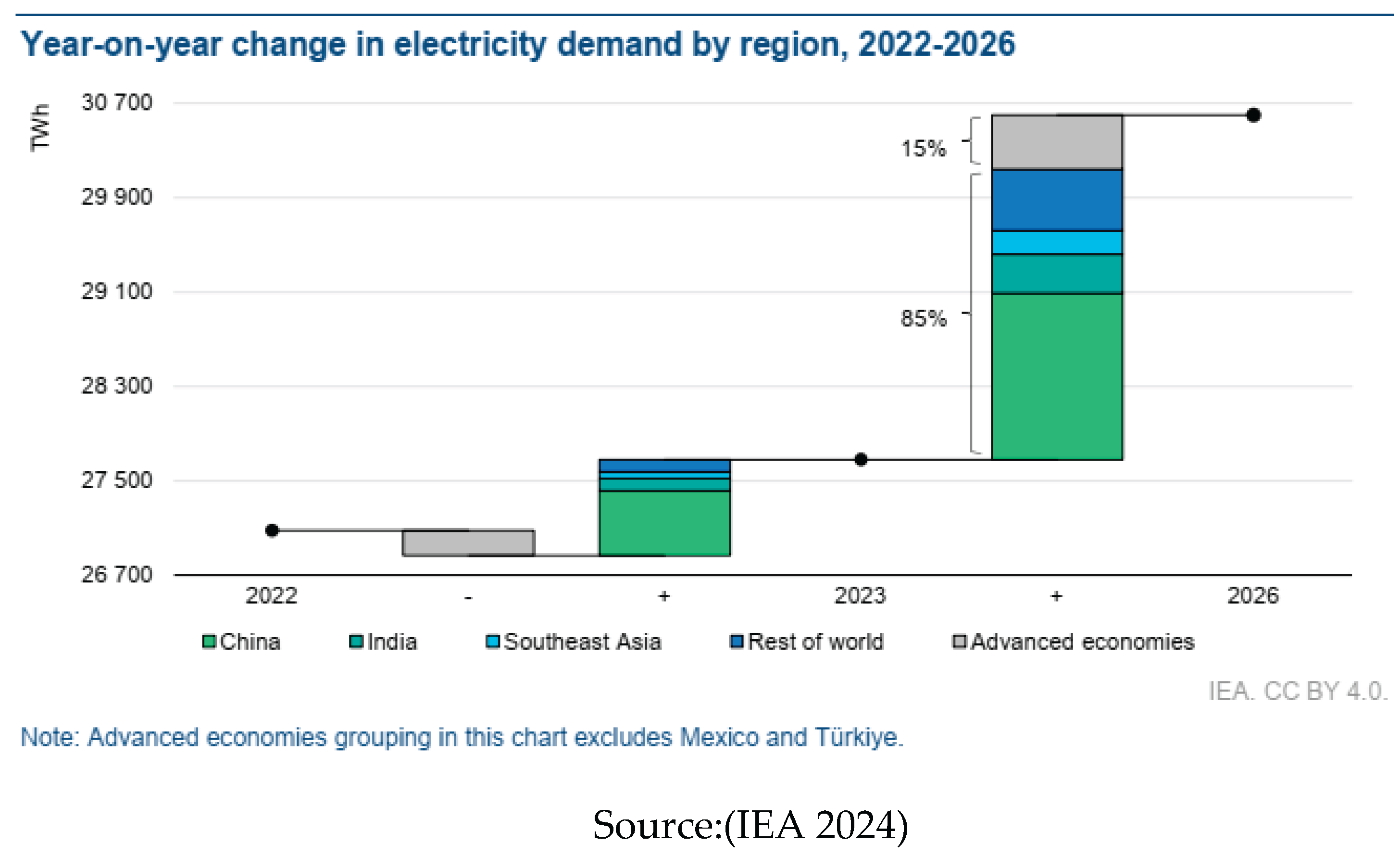
Figure 2.
Financial Development Index.
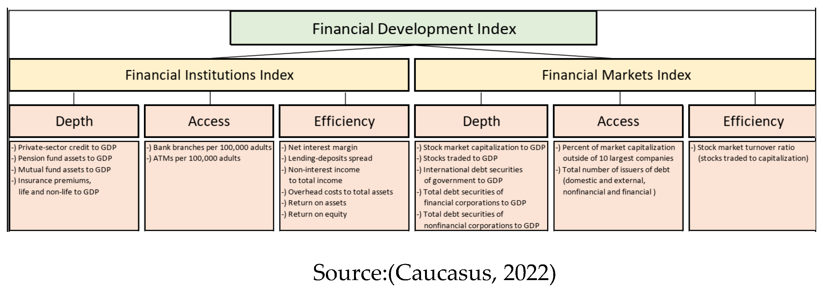
Table 1.
Summary of the Financial Development- Electricity Consumption Nexus Empirical Findings.
| Authors | Time | Countries | Methodology | Results |
|---|---|---|---|---|
| Çoban and Topcu, (2013) | 1990 – 2011 | 27 EU Countries | Sys-GMM | No effect in the 27 EU Countries. |
| Sadorsky (2010) | 1990- 2006 | 22 EMEs | Sys-GMM | Positive effect if the banking variable is used. |
| Coers & Sanders (2013) | 1960-2000 | OECD Countries | VECM | Strong unidirectional causality running from GDP to energy usage |
| Fuinhas & Marques (2012) | 1965-2009 | PIGST Countries | ARDL test | Bidirectional causality between energy and growth in both the long run and short run supports the feedback hypothesis. |
| Kahsai et al. (2012) | 1980–2007 | 40 SSA countries |
Pedroni cointegration test, Granger Causality test
|
A direct relationship between economic growth and energy demand. |
Source: Author, 2024.
Table 2.
Definition of variables and data sources.
| Variable | Definition of variables | Data Source | Expected Sign |
|---|---|---|---|
| Dependent Variable | |||
| Financial Development | The measure of breadth and depth of the financial markets is measured by the financial development index. | World Bank’s Global Financial Development Database (2023) |
N/A |
| Independent Variables | |||
| Electricity Consumption | Electricity consumption (billion kwt hr) |
International Energy Agency | +/- |
| Economic Growth | Real GDP per capita | World Development Indicators | +/- |
| FDI | Foreign Direct Investment | World Development Indicators | + |
| Government Effectiveness (GOVEFF) | Quality of Governance in a country | World Governance Indicators | + |
| Infrastructure | Total Natural Resources Rents (% of GDP) | World Development Indicators | +/- |
| Inflation | Percentage change in the GDP deflator | World Development Indicators | +/- |
| Real Interest Rates | Real interest rate % per annum | World Development Indicators | +/- |
| Resources | Total Natural Resources Rents (% of GDP) | World Development Indicators | + |
Source: Author, 2025
Table 7.
Descriptive Statistics.
| Mean | Median | Minimum | Maximum | Std, Dev, | Skewness | Kurtosis | Jarque-Bera | Observ | |
|---|---|---|---|---|---|---|---|---|---|
| FIN_DEV1 | 0,42 | 0,42 | 0,09 | 0,74 | 0,14 | 0,08 | 2,39 | 6,90 | 419 |
| ED1 | 385,61 | 123,61 | 3,38 | 7115,08 | 934,45 | 4,89 | 28,72 | 13216,14 | 419 |
| ECONGR1 | 8 264,37 | 6 141.83 | 755.48 | 59 986,44 | 9 618,28 | 3,51 | 13,50 | 4 062,22 | 419 |
| FDI | 3,08 | 219 | -40,09 | 106,60 | 7,81 | 7,76 | 93,34 | 14 6682,60 | 419 |
| GE | 0,06 | 0,00 | -1,20 | 1,51 | 0,56 | 0,34 | 2,89 | 8,08 | 419 |
| GFCF | 22,96 | 21,98 | 0,00 | 44,52 | 6,43 | 1,03 | 4,70 | 124,88 | 419 |
| INF | 8,37 | 5,90 | -16,27 | 52,98 | 8,75 | 2,08 | 9,01 | 931,51 | 419 |
| INT | 5,58 | 4,18 | -18,85 | 54,00 | 9,71 | 2,32 | 10,45 | 1346,40 | 419 |
| RES | 9,42 | 5,07 | 0,23 | 55,48 | 10,20 | 1,95 | 7,13 | 562,68 | 419 |
Source: Author’s Analysis: Descriptive statistics are calculated on all available annual data for the 2000 – 2020 period. Notes: std, Dev = Standard Deviation, Obser = Number of observations, Fin_Dev1 = Financial development index, ED1= electricity consumption (Billion KWh), EconGR1= GDP per Capita (Constant 2015 US$), ), FDI = foreign direct investment (Net inflows as a % of GDP), GE = government effectiveness, GFCF = gross fixed capital formation as a percentage of GDP, INF = inflation GDP deflator annual %, INT = real interest rates % and RES= total natural resources rents as a % of GDP.
Table 8.
Correlation Analysis.
| Variables | FIN_DEV1 | ED1 | ECONGR1 | FDI | GE | GFCF | INF | INT | LRGDP | RES |
|---|---|---|---|---|---|---|---|---|---|---|
| FIN_DEV1 | 1 | |||||||||
| ED1 | 0,2947*** | 1 | ||||||||
| ECONGR1 | -0,2951*** | -0,0408 | 1 | |||||||
| FDI | 0,0977** | -0,0323 | -0,0788 | 1 | ||||||
| GE | 0,5704*** | 0,0411 | -0,2808*** | 0,1764*** | 1 | |||||
| GFCF | 0,1923*** | 0,6141*** | 0,0432 | 0,0443 | 0,0866* | 1 | ||||
| INF | -0,2817*** | -0,1148** | 0,2122*** | -0,0759 | -0,3515*** | -0,1731*** | 1 | |||
| INT | 0,1063** | -0,042 | -0,1015** | -0,04 | -0,0566 | -0,1581*** | -0,1084** | 1 | ||
| RES | -0,0966** | -0,0936* | -0,0194 | 0,1150*** | 0,1536*** | 0,0986** | 0,0483 | 0,1266*** | -0,1276*** | 1 |
Table 9.
Summary of Pooled Mean Group on the cointegrating and causality relationship between financial development and electricity consumption.
Table 9.
Summary of Pooled Mean Group on the cointegrating and causality relationship between financial development and electricity consumption.
| PMG | PMG | PMG | PMG | |
| Variables | D.Fin_Dev1 | D.ED1 | D.EconGR1 | D.FDI |
| Long-Run | ||||
| EconGR1 | 0.0143** | 1.325*** | -0.0459 | |
| (-3.27) | (9.88) | (-0.40) | ||
| ED1 | 0.251*** | 1.596*** | 0.846 | |
| (11.34) | (4.59) | (1.04) | ||
| Fin_Dev1 | 0.0428 | 2.422 | -3.231 | |
| (1.80) | (1.65) | (-1.56) | ||
| FDI | 0.00109 | 0.0394*** | 0.0120 | |
| (1.06) | (3.97) | (0.95) | ||
| ECT | -0.299*** | -0.0538*** | -0.125*** | -0.589*** |
| (-5.33) | (-3.29) | (-3.80) | (-8.57) | |
| Short-Run | ||||
| D.EconGR1 | 0.0226 | -0.0573 | -0.226 | |
| (1.04) | (-1.19) | (-0.14) | ||
| D.ED1 | -0.249* | 0.664 | 3.677 | |
| (-2.45) | (0.67) | (0.53) | ||
| Fin_Dev1 | -0.00642 | -0.896 | 12.18 | |
| (-0.21) | (-0.83) | (1.12) | ||
| D.FDI | 0.000450 | -0.00255 | 0.0123 | |
| (0.34) | (-1.30) | (0.71) | ||
| _cons | 0.00570 | 0.0783*** | 0.0990 | 1.775* |
| (0.47) | (3.69) | (1.23) | (2.49) | |
| N | 399 | 399 | 399 | 399 |
| Hausman | 44.75*** | 39.55*** | 64.80*** | 9.42* |
Source: Author’s compilation using STATA.
Disclaimer/Publisher’s Note: The statements, opinions and data contained in all publications are solely those of the individual author(s) and contributor(s) and not of MDPI and/or the editor(s). MDPI and/or the editor(s) disclaim responsibility for any injury to people or property resulting from any ideas, methods, instructions or products referred to in the content. |
© 2025 by the authors. Licensee MDPI, Basel, Switzerland. This article is an open access article distributed under the terms and conditions of the Creative Commons Attribution (CC BY) license (http://creativecommons.org/licenses/by/4.0/).
Copyright: This open access article is published under a Creative Commons CC BY 4.0 license, which permit the free download, distribution, and reuse, provided that the author and preprint are cited in any reuse.


