Submitted:
22 July 2025
Posted:
23 July 2025
You are already at the latest version
Abstract
Aboveground biomass (AGB) in grasslands is a vital metric for assessing ecosystem functioning and health. Accurate and efficient AGB estimation is essential for the scientific management and sustainable use of grassland resources. However, achieving low-cost, high-efficiency AGB estimation via remote sensing remains a key challenge. This study integrates Sentinel-1 and Sentinel-2 imagery to derive 38 multi-source feature variables, including backscatter coefficients, texture, spectral reflectance, vegetation indices, and topographic factors. These features are combined with AGB data from 112 field plots in the Three Parallel Rivers Area. Feature selection was performed using Pearson correlation, Random Forest (RF), and SHAP values to identify optimal variable sets. Genetic Programming (GP) was then applied for nonlinear optimization of the selected features. Three machine learning models—RF, GBRT, and KNN—were used to estimate AGB and generate spatial distribution maps. Results revealed notable differences in model accuracy, with RF performing best overall, outperforming GBRT and KNN. After GP optimization, all models showed improved performance, with the RF model based on RF-selected features achieving the highest accuracy (R² = 0.90, RMSE = 0.31 t/hm², MAE = 0.23 t/hm²), improving R² by 0.03 and reducing RMSE and MAE by 0.05 and 0.03 t/hm², respectively. Spatial mapping showed AGB ranged from 0.41 to 3.59 t/hm², with a mean of 1.39 t/hm², closely aligned with the actual distribution characteristics. This study demonstrates that the RF model, combined with multi-source features and GP optimization, provides an effective approach to grassland AGB estimation and supports ecological monitoring in complex areas.
Keywords:
grassland aboveground biomass
; Sentinel-1
; Sentinel-2
; genetic programming
; machine learning
; grassland management
1. Introduction
Grassland, one of the most extensively dispersed vegetation types worldwide, comprises nearly a quarter of the land area and represents the largest terrestrial ecosystem in China. They are essential for controlling global climate, conserving soil and water, sequestering carbon, improving carbon sinks, and limiting wind erosion and desertification [1,2]. Grassland biomass consists of aboveground and belowground elements, and its geographical distribution directly affects ecosystem production. Among these, grassland aboveground biomass (AGB) serves as a vital indication of vegetation growth, carbon sequestration potential, and overall ecosystem productivity. The precise and efficient assessment of AGB is crucial for optimal grassland resource management and ecological security, offering significant data z with moderate to high plant diversity and is significantly influenced by cloud and fog cover, hence constraining estimation accuracy [11], Synthetic aperture radar (SAR) sensors, in contrast, function at longer wavelengths, remain impervious to atmospheric conditions like clouds and fog, and exhibit a degree of penetration into vegetation canopies. SAR can more efficiently acquire vegetation structure information via backscattering mechanisms linked to surface features, offering a valuable supplementary data source for biomass estimation. Prior research has shown that VH and VV polarization backscatter from Sentinel-1 SAR data exhibit significant sensitivity to the structural attributes of grasslands, hence augmenting its applicability in biomass assessment [12,13,14]. Consequently, SAR data have progressively emerged as a crucial element in grassland biomass studies.
In contrast to conventional empirical models, machine learning techniques markedly improve the precision and resilience of AGB prediction by incorporating multi-source information and elucidating nonlinear interactions among variables [15,16]. Presently, methods including K-Nearest Neighbor (KNN)[17,18], Support Vector Machine (SVM) [19,20,21], Gradient Boosting Regression Tree (GBRT) [22,23], and Random Forest (RF) [24,25,26]are extensively utilized in the remote sensing inversion of vegetation biochemical parameters. The RF approach is preferred for its robustness to outliers and high interpretability [27]; GBRT attains high accuracy with minimal parameter adjustment [28]; and KNN, which is non-parametric, excels in high-dimensional feature spaces [29]. Empirical research substantiates the efficacy of these algorithms. Mutanga et al. [30] found that in estimating AGB in South African wetlands, the RF model decreased RMSE to 0.441 kg/m², in contrast to the conventional regression method. Anderson et al. [31] attained a dependable biomass estimation (R² = 0.61) for arid steppes in southwestern Idaho, USA. Zeng et al. [32] established that RF accounted for 86% of the variance in observed AGB data for natural grasslands in central Oklahoma. Yao et al. [33] assessed grassland AGB in the Qinghai–Tibet Plateau and determined that the GBRT model utilizing 13 characteristics exhibited optimal performance (training R² = 0.79, RMSE = 43.42 g/m²). Gao et al. [34] determined that a multi-factor RF model surpassed alternative methods in calculating alpine grassland AGB. In a study of artificial grasslands in Colombia, Mendoza et al. [35] found that the KNN model was the best, achieving an R² of 0.76 and successfully predicting both AGB and dry matter (DM). These findings collectively highlight the efficacy of machine learning techniques in multi-scale AGB estimation.
The Three Parallel Rivers Area serves as a significant biological barrier in southwestern China, distinguished by intricate topography and varied ecosystems. In recent years, climate change and human activities have substantially impacted grassland degradation and heightened biomass heterogeneity. This study employs Sentinel-1 and Sentinel-2 imagery from July to September 2022, incorporating multi-source remote sensing attributes, to examine the response mechanisms grassland AGB to variables including spectral reflectance, vegetation indices, backscatter coefficients, texture features, and topographic factors. Three feature selection methodologies—Pearson, RF, and SHAP—were utilized to identify three sets of modeling characteristics. Consequently, the GP algorithm was implemented to execute nonlinear optimization of the features, and three models—RF, GBRT, and KNN—were developed for estimation. The objectives are (1) to elucidate the function of multi-source features in the inversion of grassland AGB under intricate mountainous conditions; (2) to assess the estimation accuracy of various models in complex terrain and evaluate performance discrepancies pre- and post-GP optimization; and (3) to identify the optimal model and delineate the spatial distribution of grassland AGB, thereby offering a theoretical foundation and technical assistance for regional grassland resource monitoring and ecological management.
2. Materials and Methods
2.1. Study Area
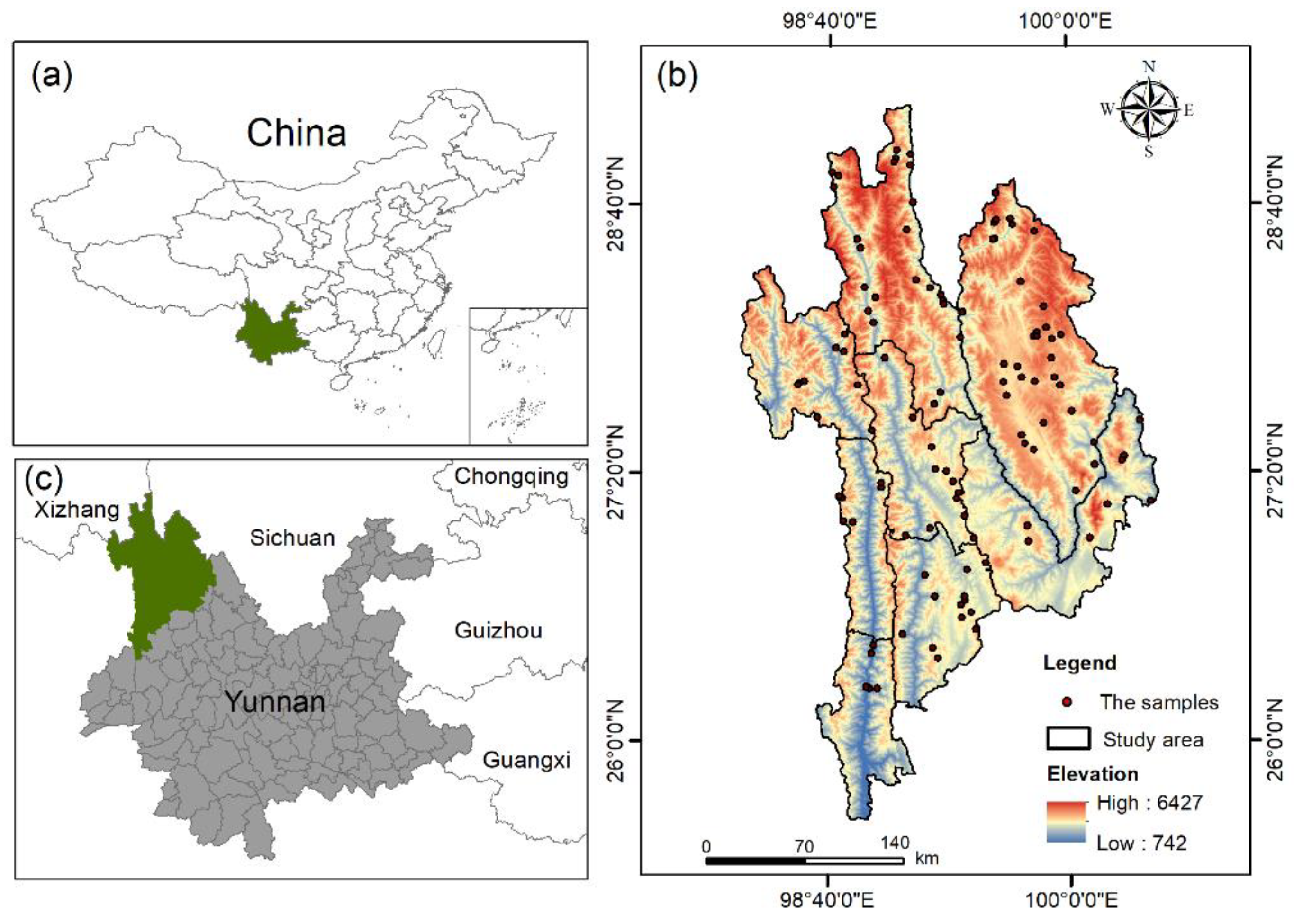
This study selected on the "Three Parallel Rivers" area in northwestern Yunnan Province, China, which includes Lushui City, Fugong County, Gongshan County, and Lanping County in Nujiang Prefecture, as well as Xianggelila City, Weixi County, Deqin County in Diqing Prefecture, and Yulong County in Lijiang City. The regional geography is intricate, including a tiered distribution with elevated terrain in the northwest and diminished altitudes in the southeast, leading to considerable altitude variations. The terrain is predominantly characterized by elevated mountain gorges. The climate displays significant vertical zonation, with annual precipitation varying from 500 to 2,000 mm, predominantly occurring between May and October, characterized by notable seasonal and geographical variability. Diverse thermal and moisture conditions have cultivated a varied array of flora types, including evergreen broadleaf forests, mixed coniferous and broadleaf forests, subalpine shrublands, and alpine meadows. Grasslands are extensively spread and are a crucial element of the alpine ecosystem, significantly contributing to regional ecological security and functionality.
Figure 1.
The location of the study area. (a) Location of the Three Parallel Rivers Area in China; (b) Distribution of 112 sample plots and DEM; (c) Location of the Three Parallel Rivers Area in Yunnan.
Figure 1.
The location of the study area. (a) Location of the Three Parallel Rivers Area in China; (b) Distribution of 112 sample plots and DEM; (c) Location of the Three Parallel Rivers Area in Yunnan.
2.2. Data Acquisition and Processing
2.2.1. Sample Plot Data
The AGB data for the study region were gathered from July to September 2022, coinciding with the peak growth phase of the grassland, hence facilitating an accurate evaluation of grassland production. A total of 118 standard circular plots, each with a radius of 40 meters and an approximate area of 0.5 hectares, were developed. Plot selection adhered to the principles of homogenous species composition, level terrain, characteristic vegetation types, and extensive dispersion to guarantee representativeness and comparability. Each plot documented data including latitude and longitude, vegetation cover, elevation, and predominant vegetation types, enabling further spatial registration and analysis.
In the sample plot, sample lines are established at three orientations: 0°, 120°, and 240°. At each endpoint, a 2 m x 2 m vegetation observation plot is established, with the diagonal aligned with the orientation of the sample line. Three yield plots measuring 1 m x 1 m were established 5 m to the right of the terminus of the sample line. The above-ground vegetation was harvested, and subsequent to the elimination of impurities and drying to a constant weight, the dry weight was ascertained. The AGB of each sample plot is the mean dry weight of three test plots. The triple standard deviation approach was employed to remove outliers, resulting in the retention of 112 plots for modeling analysis [36]. The descriptive statistics are presented in Table 1.
2.2.2. Sentinel-1 Data
Sentinel-1 is the inaugural Earth observation radar satellite mission within the European Space Agency (ESA) Copernicus Program. The system comprises two polar-orbiting satellites, Sentinel-1A and Sentinel-1B, and possesses a ground revisit capacity of six days. The C-band Synthetic Aperture Radar (SAR) it carries can penetrate clouds and conduct surface observations independently of lighting conditions. It has all-weather and all-time imaging capabilities and is particularly suitable for surface information extraction and monitoring in areas with frequent clouds and fog or complex terrain.
Sentinel-1 has many imaging modes and polarization selections. This study utilized Sentinel-1 GRD products from July to September 2022, employing VV and VH dual-polarization modes with a spatial resolution of 10 meters. The data were acquired through the Google Earth Engine (GEE) platform and subjected to standardized preprocessing, encompassing thermal noise elimination, radiometric calibration, multi-view processing, coherent spot filtering, and terrain correction, to improve data consistency and comparability.
2.2.3. Sentinel-2 Data
Sentinel-2 is the second optical Earth observation mission under the European Space Agency (ESA) Copernicus Program. It comprises two satellites, Sentinel-2A and Sentinel-2B, which together provide a revisit cycle of five days and offer multispectral imaging capabilities. It provides 13 spectrum bands, encompassing visible light, near-infrared (NIR), and short-wave infrared (SWIR) areas. The resolution for bands B2, B3, B4, and B8 is 10 meters; for bands B5, B6, B7, B8A, B11, and B12, it is 20 meters; and for bands B1, B9, and B10, it is 60 meters [13]. This study utilized surface reflectance products from the Sentinel-2 Level-2A dataset from July to September 2022, with data acquired via the GEE platform. To guarantee image quality, photos with cloud cover below 5% were filtered and consistently resampled to 10 meters for feature extraction. To address the local data loss resulting from extensive cloud cover during the summer, photos from comparable observation phases were incorporated to enhance the timeliness and spatial continuity of the data.
2.2.4. DEM Data
This study used DEM data from the SRTM global elevation product supplied by the United States Geological Survey (USGS), featuring an initial resolution of 30 meters. The DEM data were resampled to a 10-meter resolution on the GEE platform to ensure consistency with other remote sensing datasets. Thereafter, topographical metrics such as elevation, slope, and aspect were derived from the resampled DEM. This study uses small-class data from the 2022 second grassland resource survey conducted in the Three Parallel Rivers region to enhance the precision and appropriateness of grassland sample extraction for the area. A grassland distribution mask was created to eliminate non-grassland areas, thereby enhancing the accuracy and relevance of the modeling samples to the environment.
2.3. Research Methods
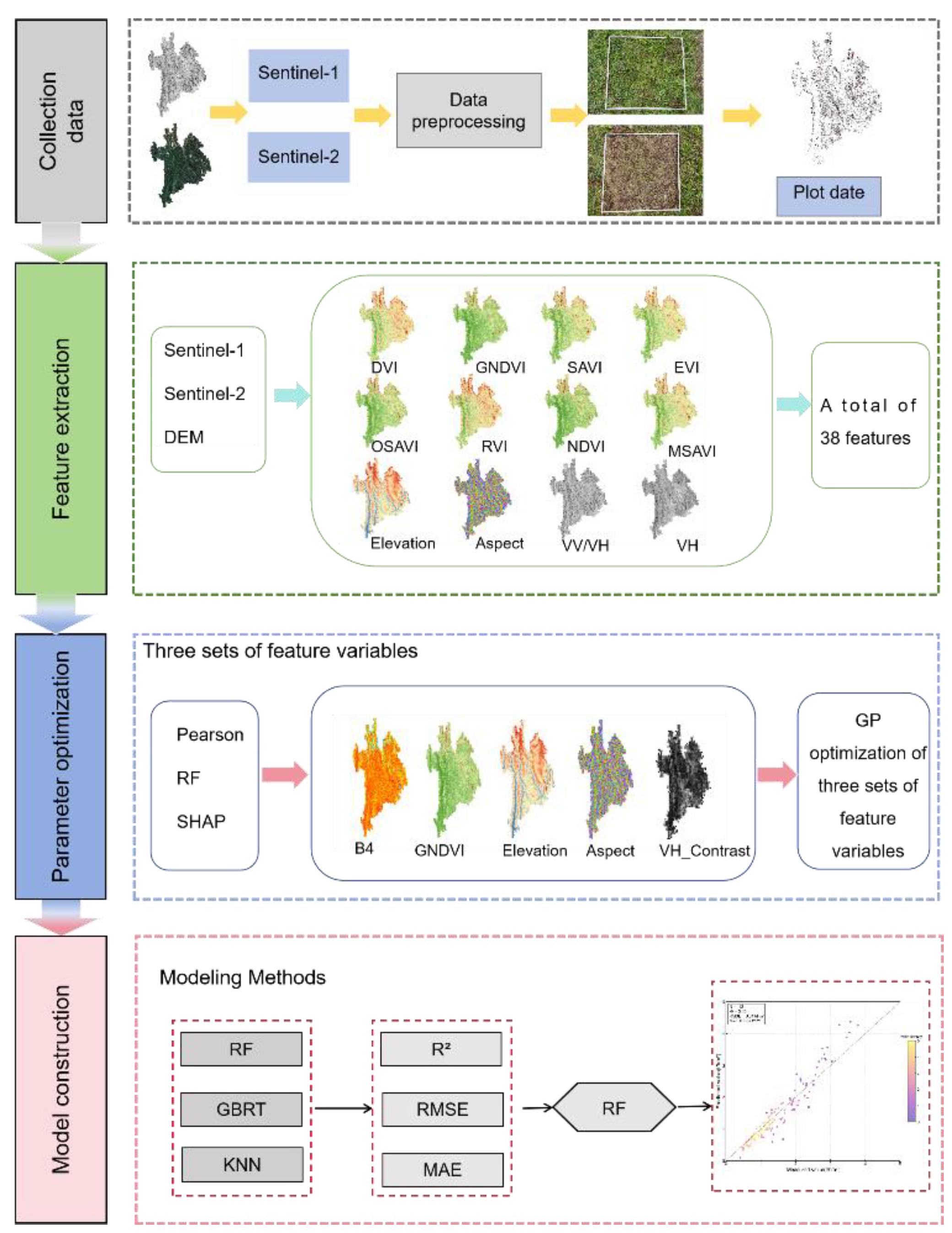
The process of inverting grassland AGB using multi-source remote sensing data includes four key steps, as described in the flowchart of Figure 3: (1) Preprocessing of Sentinel-1, Sentinel-2 and DEM data; (2) Feature selection and feature optimization; (3) Modeling of AGB in grassland ;(4) Spatial Distribution mapping of AGB in grassland.
Figure 2.
Technical route.
2.3.1. Extraction of Feature Variables
This study retrieved 38 feature variables from Sentinel-1, Sentinel-2, and DEM data to estimate the inversion of grassland AGB. Three backscatter coefficients (VV, VH, and VV/VH) and 16 texture features were extracted from Sentinel-1 imagery. The VV and VH polarization channels provided eight texture metrics to characterize the gray-level structure and surface complexity of images, effectively capturing differences in vegetation canopy structure and geographic distribution. The aim was to fully utilize the structural and spatial information contained in radar imagery concerning vegetation conditions and biomass dynamics by extracting data from various perspectives and polarization modes, thereby enhancing the model's sensitivity and predictive accuracy for grassland AGB. Table 2 presents the formulas utilized for calculating the texture attributes.
Additionally, this work obtained eight spectral reflection rates and eight vegetation cover indices from Sentinel-2 images, encompassing the visible to near-infrared bands, which effectively represent the spectral properties of vegetation. Different vegetation indices are appropriate for different types of plant cover and soil conditions, providing a complete picture of plant health and coverage (see Table 3 for the specific formulas used to calculate them).
Terrain parameters, including slope, aspect, and elevation, were derived from the DEM date to elucidate the impact of terrain on vegetation growth and biomass distribution. To align the measured plot scale with a diameter of 80 m, the average values of all feature variables were computed using an 80 m x 80 m sliding window to create the final set of modeling input variables and enhance the coherence between the features and the measured data.
2.3.2. Optimization of Modeling Feature Parameters
Significant multicollinearity among feature variables may compromise the model's predictive accuracy, increase complexity, and diminish computational efficiency. The study aimed to improve how accurately and efficiently models work by looking at how different ways of choosing features affect the remote sensing results for grassland AGB, with the goal of finding the best set of feature variables. Three feature selection methodologies—Pearson, RF, and SHAP—were implemented to identify variables significantly connected with AGB from the original feature set. The study evaluated the influence of various feature combinations on grassland AGB inversion performance by comparing estimation accuracy across different models, consequently establishing the optimal feature variable combination for the studied area.
2.3.3. Model Construction
Random Forest Regression (RF) is a bagging parallel ensemble learning technique derived from decision trees, as proposed by Breiman [27]. The primary benefit of RF is its resistance to overfitting, which allows it to handle numerous characteristics without requiring pre-selection of features during model training. RF was originally developed to improve Classification and Regression Trees (CART), allowing it to create combined predictions that make predictive models more effective [37].
Gradient Boosting Regression Tree (GBRT) [28]is an enhancement of the Boosting approach inside ensemble learning. The fundamental concept involves creating several weak classifiers and subsequently amalgamating them into a robust classifier after numerous iterations. Each training session is progressively refined based on the discrepancies of the preceding model, which continuously diminishes prediction errors and constructs a new model along the gradient direction of the minimized residuals [38,39] The GBRT model exhibits significant robustness and is capable of adapting to intricate nonlinear interactions, making it particularly effective at extracting redundant data.
K-Nearest Neighbors (KNN) regression is a widely utilized machine learning algorithm. The fundamental premise is to identify adjacent data points using distance measurements and subsequently deduce the category of the target data point based on the categorical data concerning its neighbors. The KNN approach is distinguished by its straightforward structure and capacity to concurrently estimate all variables. Compared to the independent prediction of individual variables, it more efficiently maintains the correlation and covariance structure among them [40].
2.3.4. Evaluation of Model Accuracy
Genetic Programming (GP) is an intelligent computational approach derived from the principles of biological evolution, initially introduced by Koza. As a method that uses a group of solutions to find the best one, GP can automatically create complex features from the original data by mimicking natural evolution processes such as selection, crossover, and mutation, which greatly enhance the models ability to express and generalize [41]. In contrast to conventional feature screening techniques, GP feature optimization aims not only to select subsets from existing features but also to actively investigate the potential combinations of features, uncover intricate nonlinear interactions among variables, and consequently create combined features with enhanced informational richness and modeling significance.
2.3.5. Evaluation of Model Accuracy
The study employed 10-fold cross-validation to assess the model using 112 samples, therefore minimizing data partition randomness and enhancing evaluation stability. The data was partitioned into 10 equal segments, with one segment designated as the test set and the remaining segments utilized as the training set. The process was executed ten times, and the mean value was calculated. The measures employed to assess model performance comprised the coefficient of determination (R²), root mean square error (RMSE), and mean absolute error (MAE). The pertinent formulas are as follows:
where: is the measured value; is the predicted value; is the model predicted mean; n is the sample size.
3. Results and Analysis
3.1. Correlation Coefficients and Variable Screening Results
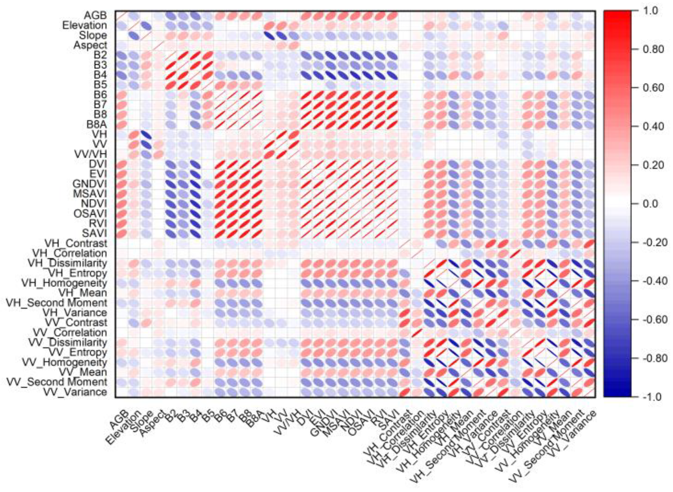
This study used Pearson, RF, and SHAP to evaluate how each characteristic variable affects grassland AGB and to find the best combination of parameters for modeling. The study selected the parameters with significant correlation as the independent variables for modeling grassland AGB from the 38 parameters analyzed. The Pearson approach established the significance threshold at 0.05, and the correlation coefficient absolute values ranged from 0.029 to 0.509. The heat map of Pearson correlation coefficients between the various characteristics and grassland AGB (Figure 3) indicates a strong association between the vegetation index and AGB. Employing a correlation coefficient threshold of 0.482, five variables exhibiting a strong association with AGB were identified: RVI (0.509), NDVI (0.493), GNDVI (0.492), OSAVI (0.488), and SAVI (0.482).
Figure 3.
Correlation matrix of each parameter of the Pearson method with grassland AGB.
This study additionally utilized RF and SHAP methodologies to evaluate and prioritize the significance of 38 feature variables. The RF analysis results (Figure 4) indicate that the variable importance varies from 0.3% to 21.3%. Five principal variables were identified with a threshold of 4%: B4 (21.3%), GNDVI (8.6%), Elevation (8.0%), Aspect (4.8%), and VH_Contrast (4.2%).
The SHAP approach was implemented to rank the significance of all feature variables, and the top 20 features were chosen for presentation (Figure 5). The findings indicate that B4, GNDVI, Elevation, B3, and B2 are among the top five variables, signifying their significant contribution to predicting grassland AGB. Consequently, the aforementioned five properties were chosen as input variables for the model to enhance modeling efficiency and minimize redundant information interference.
3.2. Model Accuracy Analysis Without GP Feature Optimization
This work employed three feature selection methods—Pearson, RF, and SHAP—to identify three distinct sets of feature variable combinations for grassland AGB modeling. Three models—RF, GBRT, and KNN—were then created to estimate grassland AGB using remote sensing in the Three Parallel Rivers area. Figure 6 illustrates that the RF model exhibited enhanced predictive accuracy, with R² = 0.87, RMSE = 0.35 t/hm², and MAE = 0.26 t/hm², surpassing the estimate capabilities of the GBRT and KNN models.
3.3. Analysis of Model Accuracy After GP Feature Optimization
To improve the inversion accuracy of grassland AGB, three groups of modeling variables were chosen using Pearson, RF, and SHAP feature selection methods. The GP method was then used to improve the three sets of features, leading to the creation of a remote sensing model for measuring grassland AGB in the Three Parallel Rivers area. Figure 7 shows that after using GP optimization, each model's ability to make accurate predictions improved, confirming that GP is effective in enhancing how well features are represented. The RF model utilizing RF feature selection and optimized by GP exhibited the highest performance, with R² = 0.90, RMSE = 0.31 t/hm², and MAE = 0.23 t/hm². In comparison to the pre-optimization results, R² rose by 0.03, RMSE diminished by 0.05, and MAE reduced by 0.03, indicating robust predictive capability and stability.
Further analysis based on Table 4 and Figure 7, from a vertical perspective, the identical set of feature variables displays notable performance disparities among various models, with the RF model exhibiting generally greater predictive efficacy relative to GBRT and KNN. From a horizontal viewpoint, the identical model demonstrates performance variations across distinct feature combinations. The feature variables identified by the RF and SHAP approaches exhibit enhanced modeling performance relative to the conventional Pearson method. Thorough comparisons reveal that the RF feature combinations refined by GP exhibit superior adaptability and expressive capability across multiple models.
To enhance the validation of the model predictive capability, Figure 8 illustrates a comparison between the trends of the predicted values and the actual measured values of the RF model subsequent to RF feature selection and GP optimization. The two trends are fundamentally consistent, demonstrating that the RF model can accurately flip the AGB changing pattern and exhibits great predictive accuracy. This further substantiates that the GP feature-optimized model exhibits strong generalization capability and stability.
3.4. Spatial Distribution of Grassland AGB in the Three Parallel Rivers Area
The best RF model, chosen through RF feature screening and refined using GP, effectively inverted the spatial distribution pattern of grassland AGB in the Three Parallel Rivers Region (Figure 9). The findings indicated that the AGB range in the study area was from 0.41 to 3.59 t/hm², with a mean value of 1.39 t/hm², demonstrating considerable spatial variation. The northwestern region is in the central longitudinal valley of the Hengduan Mountains, distinguished by fragmented topography, considerable elevation fluctuations, and an inhospitable climate, leading to restricted vegetation development and typically low AGB values, predominantly comprising alpine meadows and shrub grasslands. The southeastern Shangri-La region has mostly flat land and good water and temperature conditions, which leads to a lot of grasslands and much higher AGB values, especially around Napa Lake Wetland. In the central region extending from Weixi to the southwestern area of Lanping, AGB exhibits an increasing trend from west to east, shaped by the topography of the Lancang River valley and vertical climatic variation. The South Asian monsoon affects the eastern region, providing ample water and heat resources conducive to grassland development and biomass accumulation. In the southern region, including the southern portion of Yulong County and places south of Lushui County, grasslands are fragmented, human activities are prevalent, and AGB is often low, exhibiting a distinct clustering of diminished values. The research area demonstrates considerable geographic variation in AGB, characterized by the distribution of high-value zones in patches, while the overall biomass level remains relatively low, indicative of the typical spatial attributes of a high-altitude ecosystem. The RF model inversion results exhibit strong alignment with the real distribution features, confirming its flexibility and estimating proficiency in intricate mountainous settings.
4. Discussion
4.1. Selection of Characteristic Variables and Sensitivity Analysis
In the process of remote sensing the inversion of grassland AGB, spectral reflectance and vegetation indices serve as the key inputs for inversion models, with their selection and combination directly influencing the model's structure and predictive accuracy. This study combined Pearson, RF, and SHAP methodologies to evaluate 38 multi-source remote sensing feature variables and developed three sets of modeling variable combinations. The findings demonstrate that various feature selection techniques display distinct disparities in variable ranking and model efficacy. The RF method, an ensemble learning algorithm, is capable of managing high-dimensional nonlinear data. The variables chosen by this strategy exhibit enhanced interpretability and stability in subsequent model training, leading to improved predictive performance. Concurrently, the SHAP methodology displays a notable advantage in elucidating feature contributions, showcasing superior interpretability. Figure 5 illustrates that the five most significant variables identified by SHAP (B4, GNDVI, Elevation, B3, and B2) encompass several informational dimensions, including vegetation spectral features and topography, thereby exhibiting robust comprehensive representativeness. The Pearson approach, which relies on linear correlation, is highly efficient; yet, it fails to represent nonlinear interactions adequately between variables, leading to comparatively diminished modeling accuracy in variable selection. This suggests that, when estimating grassland AGB in complicated terrains, the integration of nonlinear approaches for feature evaluation is more beneficial and establishes a robust basis for future feature optimization and modeling.
4.2. GP Feature Optimization Improves Model Accuracy
To further improve model performance, the study implemented the GP algorithm, with three feature sets, to enhance model performance and reveal potential nonlinear correlations among variables through nonlinear optimization. The optimization findings indicated that the accuracy of all models enhanced following GP feature optimization, hence affirming the beneficial impact of feature optimization on the models. The RF model utilizing RF features and optimized by GP exhibited the highest performance, achieving an R² of 0.90, with RMSE and MAE reduced to 0.31 t/hm² and 0.23 t/hm², respectively. These results reflect enhancements of 0.03 and reductions of 0.05 t/hm² and 0.03 t/hm², respectively, in comparison to pre-optimization, indicating superior prediction accuracy and stability. Notably, despite the relatively poor modeling accuracy of the original features picked via the Pearson approach, the accuracy of the KNN model developed post-GP optimization exhibited the most substantial enhancement, with R² rising from 0.43 to 0.49. This suggests that GP partially mitigates the shortcomings of conventional linear feature selection methods, adeptly revealing potential nonlinear interactions among variables and improving the model's capacity to address intricate ecological processes. In steep canyon regions with fragmented terrain and significant altitude variations, such as the Three Parallel Rivers area, conventional modeling techniques encounter difficulties due to elevated data noise and intricate variable interaction processes. The nonlinear feature combinations generated by GP optimization may proficiently adjust to the intricate coupling interactions among multi-source data, exhibiting enhanced flexibility and resilience in complicated terrain situations.
In summary, GP optimization enhances modeling accuracy and generalization capabilities while offering a dependable method for the collaborative modeling of multi-source remote sensing data in intricate mountainous ecosystems, showcasing significant practical application potential and promotional value.
4.3. The Enhancement Effect of Multi-Source Data Fusion on the Inversion of AGB in Grassland
The choice of data sources significantly influences the accuracy of models in the remote sensing inversion of grassland AGB. This research combined Sentinel-1 radar, Sentinel-2 optical, and DEM data to derive 38 multi-source feature variables, encompassing backscatter coefficient, textural characteristics, spectral reflectance, vegetation indices, and topographical aspects. Diverse feature types offer supplementary insights into vegetation structure, spectral response, and habitat circumstances, hence augmenting the model's capacity to delineate the geographic heterogeneity of grassland biomass. Prior research has demonstrated that AGB estimation algorithms reliant on a singular data source have significant limitations. For instance, Guerini Filho et al. [42]calculated the R² of AGB for the Pampa grassland in Brazil using Sentinel-2 to be merely 0.51, Song et al. [43] established the R² of the AGB model for Tibet grassland using MODIS data to be 0.60. In contrast, this study combines Sentinel-1 radar, Sentinel-2 optical, and DEM data to develop a multi-source remote sensing estimation model, achieving a R² of 0.90, which markedly surpasses prior results, thereby confirming the benefits of multi-source fusion in enhancing accuracy and robustness.
Optical features, including B4 and GNDVI, demonstrate significant sensitivity in indicating vegetation chlorophyll content and spectral absorption. Radar backscatter coefficients, such as VV and VH, along with their texture information, effectively enhance data on vegetation structure and canopy roughness, rendering them especially appropriate for monitoring intricate terrains or overcast regions. The findings align with the conclusions of Su and Vahidi et al. [44,45], further substantiating the efficacy of SAR data in assessing vegetation structure and moisture levels in fragmented terrains. The elevation and slope orientation in DEMs indicate the essential regulatory influence of hydrological patterns and vegetation distribution.
Furthermore, distinct modeling techniques demonstrate disparate reactions to multi-source features. The RF model excels in managing high-dimensional heterogeneous data, GBRT is more responsive to combinations of continuous variables, and KNN relies heavily on the amount and quality of features. Multi-source fusion enriches input variable information and enhances modeling stability and generalization capabilities, establishing a dependable foundation for high-precision retrieval of grassland AGB in complicated terrain regions.
5. Conclusions
- (1)
- This study developed a system for estimating grassland AGB with multi-source remote sensing data fusion, incorporating Sentinel-1, Sentinel-2, and DEM data to derive 38 feature variables. Feature selection was conducted using three methods: Pearson, RF, and SHAP. Based on this, feature optimization was executed utilizing the GP algorithm, while modeling and comparative analysis were carried out employing three models: RF, GBRT, and KNN. The primary conclusions are as follows:
- (2)
- Results of feature selection indicate that various strategies differ in their capacity for variable selection and modeling adaptability. The features selected by the RF and SHAP approaches exhibit high performance across several models, demonstrating enhanced modeling stability and adaptability.
- (3)
- The model comparison findings indicate that the incorporation of the GP method to optimize the three feature sets enhanced the accuracy of each model to differing extents. The RF model that used RF features and was improved by GP performed better, reaching an R² of 0.90, with RMSE and MAE lowered to 0.31 t/hm² and 0.23 t/hm², showing that GP effectively improved how features are represented and how well the model works overall.
- (4)
- Spatial inversion results indicate that the AGB of grasslands in the Three Parallel Rivers Area generally escalates from northwest to southeast, ranging from 0.41 to 3.59 t/hm², with a mean value of 1.39 t/hm². The northwest features steep topography and a frigid environment, leading to diminished AGB levels; conversely, the southeast possesses comparatively moderate terrain and advantageous water and thermal conditions, resulting in markedly elevated AGB levels. In comparison to northern China's grasslands, the overall biomass of grasslands in this region is comparatively low, indicating disparities in ecological structure and the supply and demand of resources between northern and southern grasslands.
- (5)
- The integrated modeling framework established in this study exhibits strong adaptation and resilience in complicated terrain, offering technical assistance for grassland resource monitoring and ecological management in highland mountainous environments. In the future, ecological variables, including meteorological, soil, and phenological data, together with time series data, may be integrated to improve the models spatio-temporal generality and predictive accuracy.
Author Contributions
Conceptualization, R.W., Z.L. and L.F.; methodology, R.W. and Q.S.; software, R.W., Z.L. and Q.X.; formal analysis, R.W. and L.F.; investigation, R.W. and Q.S.; resources, Q.S., X.R. and J.L.; data curation, Q.S.; writing—original draft preparation, R.W.; writing—review and editing, R.W., Q.S., Z.L., L.F., Q.X., and C.Q.; visualization, Q.S.; supervision, Q.S., C.Q., X.R. and J.L.; project administration, R.W. and Q.S.; funding acquisition, Q.S. All authors have read and agreed to the published version of the manuscript.
Funding
This study was supported by the Joint Agricultural Project of Yunnan Province (Nos. 202301BD070001-002), and the National Natural Science Foundation of China (Nos. 3186020).
Data Availability Statement
The Sentinel-1, Sentinel-2, and DEM data used in this study were obtained through the Google Earth Engine (GEE) platform (https://earthengine.google.com/, accessed on February 25, 2025). Relevant actual measurement data can be obtained from the corresponding author upon reasonable request.
Conflicts of Interest
The authors declare no conflicts of interest.
Abbreviations
The following abbreviations are used in this manuscript:
| AGB | Aboveground biomass |
| DEM | Digital Elevation Model |
| GP | Genetic Programming |
References
- John, R.; Chen, J.; Giannico, V.; Park, H.; Xiao, J.; Shirkey, G.; Ouyang, Z.; Shao, C.; Lafortezza, R.; Qi, J. Grassland Canopy Cover and Aboveground Biomass in Mongolia and Inner Mongolia: Spatiotemporal Estimates and Controlling Factors. Remote Sens. Environ. 2018, 213, 34–48. [Google Scholar] [CrossRef]
- Sun, Y.; Yang, Y.; Zhao, X.; Tang, Z.; Wang, S.; Fang, J. Global Patterns and Climatic Drivers of Above-and Belowground Net Primary Productivity in Grasslands. Sci. China Life Sci. 2021, 64, 739–751. [Google Scholar] [CrossRef] [PubMed]
- Gao, T.; Yang, X.; Jin, Y.; Ma, H.; Li, J.; Yu, H.; Yu, Q.; Zheng, X.; Xu, B. Spatio-Temporal Variation in Vegetation Biomass and Its Relationships with Climate Factors in the Xilingol Grasslands, Northern China. PLOS One 2013, 8, e83824. [Google Scholar] [CrossRef] [PubMed]
- Quan, X.; He, B.; Yebra, M.; Yin, C.; Liao, Z.; Zhang, X.; Li, X. A Radiative Transfer Model-Based Method for the Estimation of Grassland Aboveground Biomass. Int. J. Appl. Earth Obs. Geoinformation 2017, 54, 159–168. [Google Scholar] [CrossRef]
- Lu, D. The Potential and Challenge of Remote Sensing-based Biomass Estimation. Int. J. Remote Sens. 2006, 27, 1297–1328. [Google Scholar] [CrossRef]
- Li, F.; Zeng, Y.; Luo, J.; Ma, R.; Wu, B. Modeling Grassland Aboveground Biomass Using a Pure Vegetation Index. Ecol. Indic. 2016, 62, 279–288. [Google Scholar] [CrossRef]
- Schulze-Brüninghoff, D.; Hensgen, F.; Wachendorf, M.; Astor, T. Methods for LiDAR-Based Estimation of Extensive Grassland Biomass. Comput. Electron. Agric. 2019, 156, 693–699. [Google Scholar] [CrossRef]
- Pang, H.; Zhang, A.; Kang, X.; He, N.; Dong, G. Estimation of the Grassland Aboveground Biomass of the Inner Mongolia Plateau Using the Simulated Spectra of Sentinel-2 Images. Remote Sens. 2020, 12, 4155. [Google Scholar] [CrossRef]
- Li, C.; Zhou, L.; Xu, W. Estimating Aboveground Biomass Using Sentinel-2 MSI Data and Ensemble Algorithms for Grassland in the Shengjin Lake Wetland, China. Remote Sens. 2021, 13, 1595. [Google Scholar] [CrossRef]
- Shoko, C.; Mutanga, O.; Dube, T. Progress in the Remote Sensing of C3 and C4 Grass Species Aboveground Biomass over Time and Space. ISPRS J. Photogramm. Remote Sens. 2016, 120, 13–24. [Google Scholar] [CrossRef]
- Eisfelder, C.; Kuenzer ,Claudia; and Dech, S. Derivation of Biomass Information for Semi-Arid Areas Using Remote-Sensing Data. Int. J. Remote Sens. 2012, 33, 2937–2984. [CrossRef]
- Barrett, B.; Nitze, I.; Green, S.; Cawkwell, F. Assessment of Multi-Temporal, Multi-Sensor Radar and Ancillary Spatial Data for Grasslands Monitoring in Ireland Using Machine Learning Approaches. Remote Sens. Environ. 2014, 152, 109–124. [Google Scholar] [CrossRef]
- Wang, J.; Xiao, X.; Bajgain, R.; Starks, P.; Steiner, J.; Doughty, R.B.; Chang, Q. Estimating Leaf Area Index and Aboveground Biomass of Grazing Pastures Using Sentinel-1, Sentinel-2 and Landsat Images. ISPRS J. Photogramm. Remote Sens. 2019, 154, 189–201. [Google Scholar] [CrossRef]
- Komisarenko, V.; Voormansik, K.; Elshawi, R.; Sakr, S. Exploiting Time Series of Sentinel-1 and Sentinel-2 to Detect Grassland Mowing Events Using Deep Learning with Reject Region. Sci. Rep. 2022, 12, 983. [Google Scholar] [CrossRef] [PubMed]
- Belgiu, M.; Drăguţ, L. Random Forest in Remote Sensing: A Review of Applications and Future Directions. ISPRS J. Photogramm. Remote Sens. 2016, 114, 24–31. [Google Scholar] [CrossRef]
- Wolanin, A.; Camps-Valls, G.; Gómez-Chova, L.; Mateo-García, G.; van der Tol, C.; Zhang, Y.; Guanter, L. Estimating Crop Primary Productivity with Sentinel-2 and Landsat 8 Using Machine Learning Methods Trained with Radiative Transfer Simulations. Remote Sens. Environ. 2019, 225, 441–457. [Google Scholar] [CrossRef]
- Jia, Z.; Zhang, Z.; Cheng, Y.; Buhebaoyin; Borjigin, S.; Quan, Z. Grassland Biomass Spatiotemporal Patterns and Response to Climate Change in Eastern Inner Mongolia Based on XGBoost Model Estimates. Ecol. Indic. 2024, 158, 111554. [CrossRef]
- Yang, H.; Qin, Z.; Shu, Q.; Xu, L.; Yu, J.; Luo, S.; Wu, Z.; Xia, C.; Yang, Z. Estimation of Above-Ground Biomass for Dendrocalamus Giganteus Utilizing Spaceborne LiDAR GEDI Data. IEEE J. Sel. Top. Appl. Earth Obs. Remote Sens. 2025, 18, 5271–5286. [Google Scholar] [CrossRef]
- Dusseux, P.; Corpetti, T.; Hubert-Moy, L.; Corgne, S. Combined Use of Multi-Temporal Optical and Radar Satellite Images for Grassland Monitoring. Remote Sens. 2014, 6, 6163–6182. [Google Scholar] [CrossRef]
- Zhang, B.; Zhang, L.; Xie, D.; Yin, X.; Liu, C.; Liu, G. Application of Synthetic NDVI Time Series Blended from Landsat and MODIS Data for Grassland Biomass Estimation. Remote Sens. 2016, 8, 10. [Google Scholar] [CrossRef]
- Meng, B.; Liang, T.; Yi, S.; Yin, J.; Cui, X.; Ge, J.; Hou, M.; Lv, Y.; Sun, Y. Modeling Alpine Grassland above Ground Biomass Based on Remote Sensing Data and Machine Learning Algorithm: A Case Study in East of the Tibetan Plateau, China. IEEE J. Sel. Top. Appl. Earth Obs. Remote Sens. 2020, 13, 2986–2995. [Google Scholar] [CrossRef]
- Xia, C.; Zhou, W.; Shu, Q.; Wu, Z.; Wang, M.; Xu, L.; Yang, Z.; Yu, J.; Song, H.; Duan, D. Unlocking Vegetation Health: Optimizing GEDI Data for Accurate Chlorophyll Content Estimation. Front. Plant Sci. 2024, 15, 1492560. [Google Scholar] [CrossRef] [PubMed]
- Qin, Z.; Yang, H.; Shu, Q.; Yu, J.; Yang, Z.; Ma, X.; Duan, D. Estimation of Dendrocalamus Giganteus Leaf Area Index by Combining Multi-Source Remote Sensing Data and Machine Learning Optimization Model. Front. Plant Sci. 2025, 15, 1505414. [Google Scholar] [CrossRef] [PubMed]
- Ge, J.; Hou, M.; Liang, T.; Feng, Q.; Meng, X.; Liu, J.; Bao, X.; Gao, H. Spatiotemporal Dynamics of Grassland Aboveground Biomass and Its Driving Factors in North China over the Past 20 Years. Sci. Total Environ. 2022, 826, 154226. [Google Scholar] [CrossRef] [PubMed]
- Wang, Y.; Qin, R.; Cheng, H.; Liang, T.; Zhang, K.; Chai, N.; Gao, J.; Feng, Q.; Hou, M.; Liu, J.; et al. Can Machine Learning Algorithms Successfully Predict Grassland Aboveground Biomass? Remote Sens. 2022, 14, 3843. [Google Scholar] [CrossRef]
- Zhi, Q.; Hu, X.; Wang, P.; Li, M.; Ding, Y.; Wu, Y.; Peng, T.; Li, W.; Guan, X.; Shi, X.; et al. Estimation, Spatiotemporal Dynamics, and Driving Factors of Grassland Biomass Carbon Storage Based on Machine Learning Methods: A Case Study of the Hulunbuir Grassland. Remote Sens. 2024, 16, 3709. [Google Scholar] [CrossRef]
- Breiman, L. Random Forests. Mach. Learn. 2001, 45, 5–32. [Google Scholar] [CrossRef]
- Friedman, J.H. Greedy Function Approximation: A Gradient Boosting Machine. Ann. Stat. 2001, 29, 1189–1232. [Google Scholar] [CrossRef]
- Sun, H.; Wang, Q.; Wang, G.; Lin, H.; Luo, P.; Li, J.; Zeng, S.; Xu, X.; Ren, L. Optimizing kNN for Mapping Vegetation Cover of Arid and Semi-Arid Areas Using Landsat Images. Remote Sens. 2018, 10, 1248. [Google Scholar] [CrossRef]
- Mutanga, O.; Adam, E.; Cho, M.A. High Density Biomass Estimation for Wetland Vegetation Using WorldView-2 Imagery and Random Forest Regression Algorithm. Int. J. Appl. Earth Obs. Geoinformation 2012, 18, 399–406. [Google Scholar] [CrossRef]
- Anderson, K.E.; Glenn, N.F.; Spaete, L.P.; Shinneman, D.J.; Pilliod, D.S.; Arkle, R.S.; McIlroy, S.K.; Derryberry, D.R. Estimating Vegetation Biomass and Cover across Large Plots in Shrub and Grass Dominated Drylands Using Terrestrial Lidar and Machine Learning. Ecol. Indic. 2018, 84, 793–802. [Google Scholar] [CrossRef]
- Zeng, N.; Ren, X.; He, H.; Zhang, L.; Zhao, D.; Ge, R.; Li, P.; Niu, Z. Estimating Grassland Aboveground Biomass on the Tibetan Plateau Using a Random Forest Algorithm. Ecol. Indic. 2019, 102, 479–487. [Google Scholar] [CrossRef]
- Yao, Y.; Ren, H. Estimation of grassland aboveground biomass on the Qinghai-Tibet Plateau. Acta Ecologica Sinica. 2024, 44, 3049–3059. [Google Scholar] [CrossRef]
- Gao, X.; Dong, S.; Li, S.; Xu, Y.; Liu, S.; Zhao, H.; Yeomans, J.; Li, Y.; Shen, H.; Wu, S.; et al. Using the Random Forest Model and Validated MODIS with the Field Spectrometer Measurement Promote the Accuracy of Estimating Aboveground Biomass and Coverage of Alpine Grasslands on the Qinghai-Tibetan Plateau. Ecol. Indic. 2020, 112, 106114. [Google Scholar] [CrossRef]
- Alvarez-Mendoza, C.I.; Guzman, D.; Casas, J.; Bastidas, M.; Polanco, J.; Valencia-Ortiz, M.; Montenegro, F.; Arango, J.; Ishitani, M.; Selvaraj, M.G. Predictive Modeling of Above-Ground Biomass in Brachiaria Pastures from Satellite and UAV Imagery Using Machine Learning Approaches. Remote Sens. 2022, 14, 5870. [Google Scholar] [CrossRef]
- Göttsche, F.-M.; Olesen, F.-S.; Bork-Unkelbach, A. Validation of Land Surface Temperature Derived from MSG/SEVIRI within Situmeasurements at Gobabeb, Namibia. Int. J. Remote Sens. 2012, 34, 3069–3083. [Google Scholar] [CrossRef]
- Breiman, L. Bagging Predictors. Mach. Learn. 1996, 24, 123–140. [Google Scholar] [CrossRef]
- Zhang, H.; Liu, W.; Han, W.; Liu, Q.; Song, R.; Hou, G. Inversion of Summer Maize Leaf Area Index Based on Gradient Boosting Decision Tree Algorithm. Transactions of the Chinese Society for Agricultural Machinery.2019, 50(5),251-259. [CrossRef]
- Li, J.; Zhang, Y.; Liu, Y. Forest Height Estimation Method Based on Kernel Gradient Boosting Decision Tree. Journal of Beijing University of Technology. 2021,47(11),1113-1121. [CrossRef]
- Gjertsen, A.K. Accuracy of Forest Mapping Based on Landsat TM Data and a kNN-Based Method. Remote Sens. Environ. 2007, 110, 420–430. [Google Scholar] [CrossRef]
- Koza, J.R. Genetic Programming : On the Programming of Computers by Means of Natural Selection; Cambridge, Mass. : MIT Press, 1992; ISBN 978-0-262-11170-6.
- Guerini Filho, M.; Kuplich ,Tatiana Mora; and Quadros, F.L.F.D. Estimating Natural Grassland Biomass by Vegetation Indices Using Sentinel 2 Remote Sensing Data. Int. J. Remote Sens. 2020, 41, 2861–2876. [CrossRef]
- Song, K.; Jiang, F.; Hu, Z.; Lv, Y.; Long, Y.; Deng, M.; Chen, S.; Sun, H. Remote sensing inversion of above-ground biomass of grassland in the Tibet Autonomous Region. Acta Ecologica Sinica. 2023, 43(14), 5600-5613. [CrossRef]
- Sun, J.; Du, Z.; Lin, Y.; Wang, J. Inversion of aboveground biomass of grassland on the eastern margin of the Qinghai-Tibet Plateau combined with Sentinel-1andSentinel-2 data. Pratacultural Science. 2023, 40(8),1977-1987. [CrossRef]
- Vahidi, M.; Shafian, S.; Thomas, S.; Maguire, R. Estimation of Bale Grazing and Sacrificed Pasture Biomass through the Integration of Sentinel Satellite Images and Machine Learning Techniques. Remote Sens. 2023, 15, 5014. [Google Scholar] [CrossRef]
Figure 4.
Contribution ratio of the importance of each parameter feature in RF feature selection.
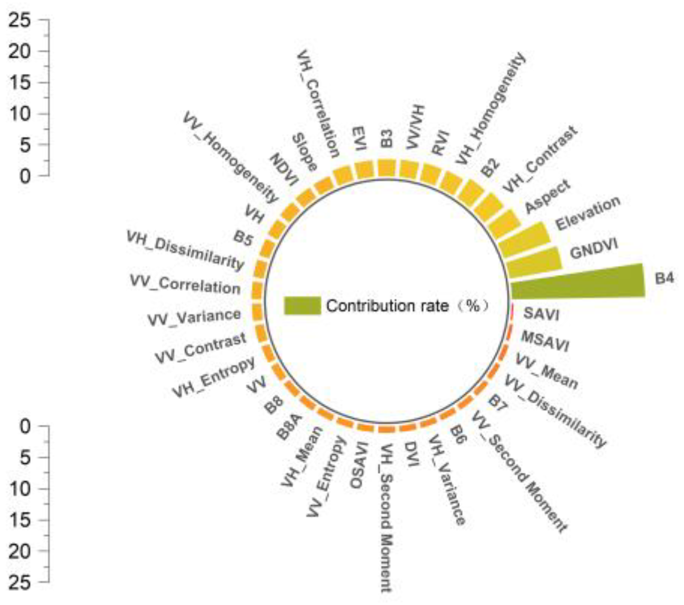
Figure 5.
SHAP feature selection parameter importance ranking: (a) Ranking of the absolute influence range of individual variables on the SHAP value of the model; (b) Ranking of the average absolute value of all variables on the SHAP value of the model.
Figure 5.
SHAP feature selection parameter importance ranking: (a) Ranking of the absolute influence range of individual variables on the SHAP value of the model; (b) Ranking of the average absolute value of all variables on the SHAP value of the model.
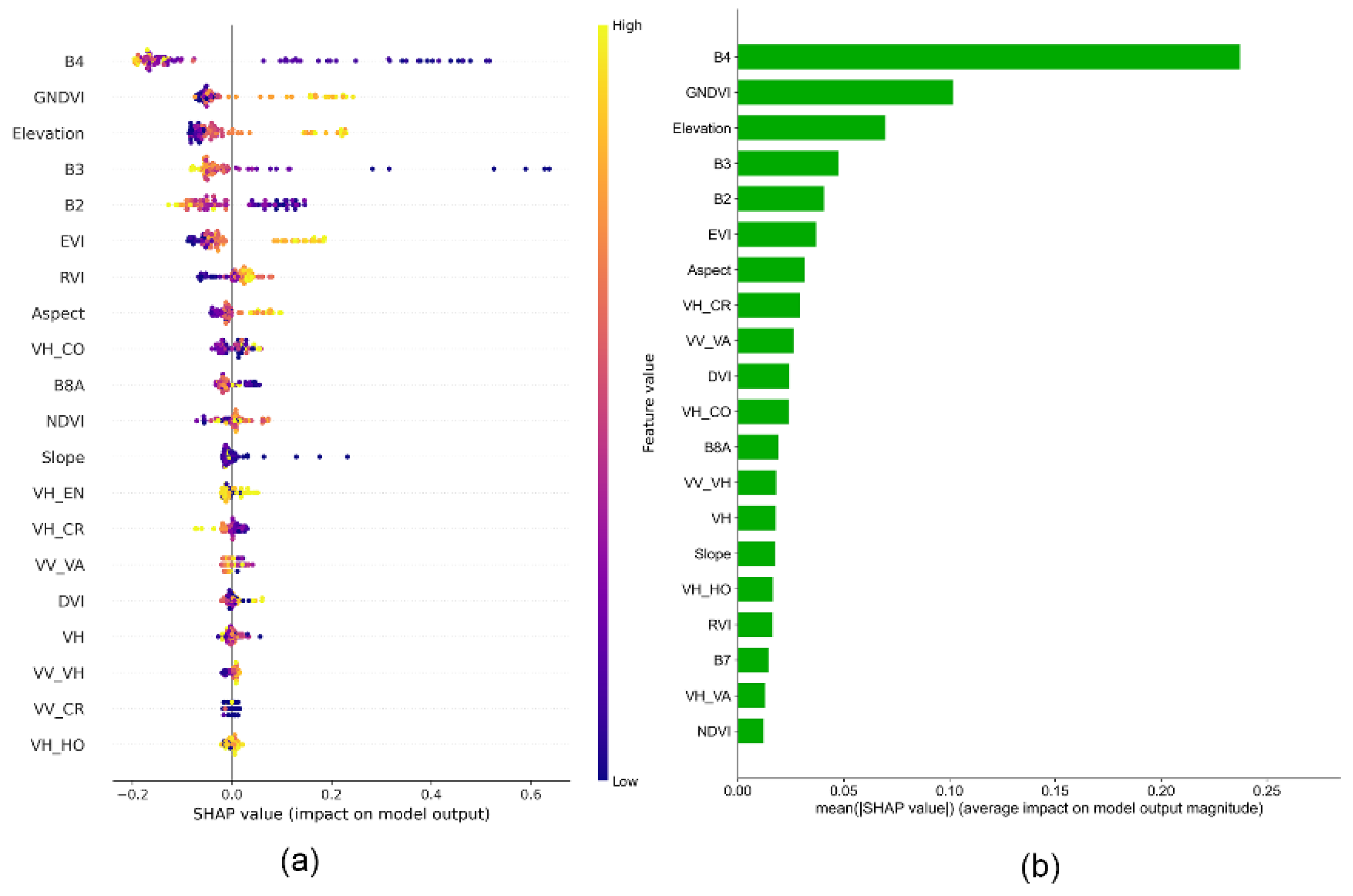
Figure 6.
Comparison of the accuracy of different models: In the horizontal direction, the three models are RF, KNN, and GBRT, and the three groups of feature variables are Pearson, RF, and SHAP. In the vertical direction, the three groups of feature variables are Pearson, RF, and SHAP, and the three models are RF, KNN, and GBRT.
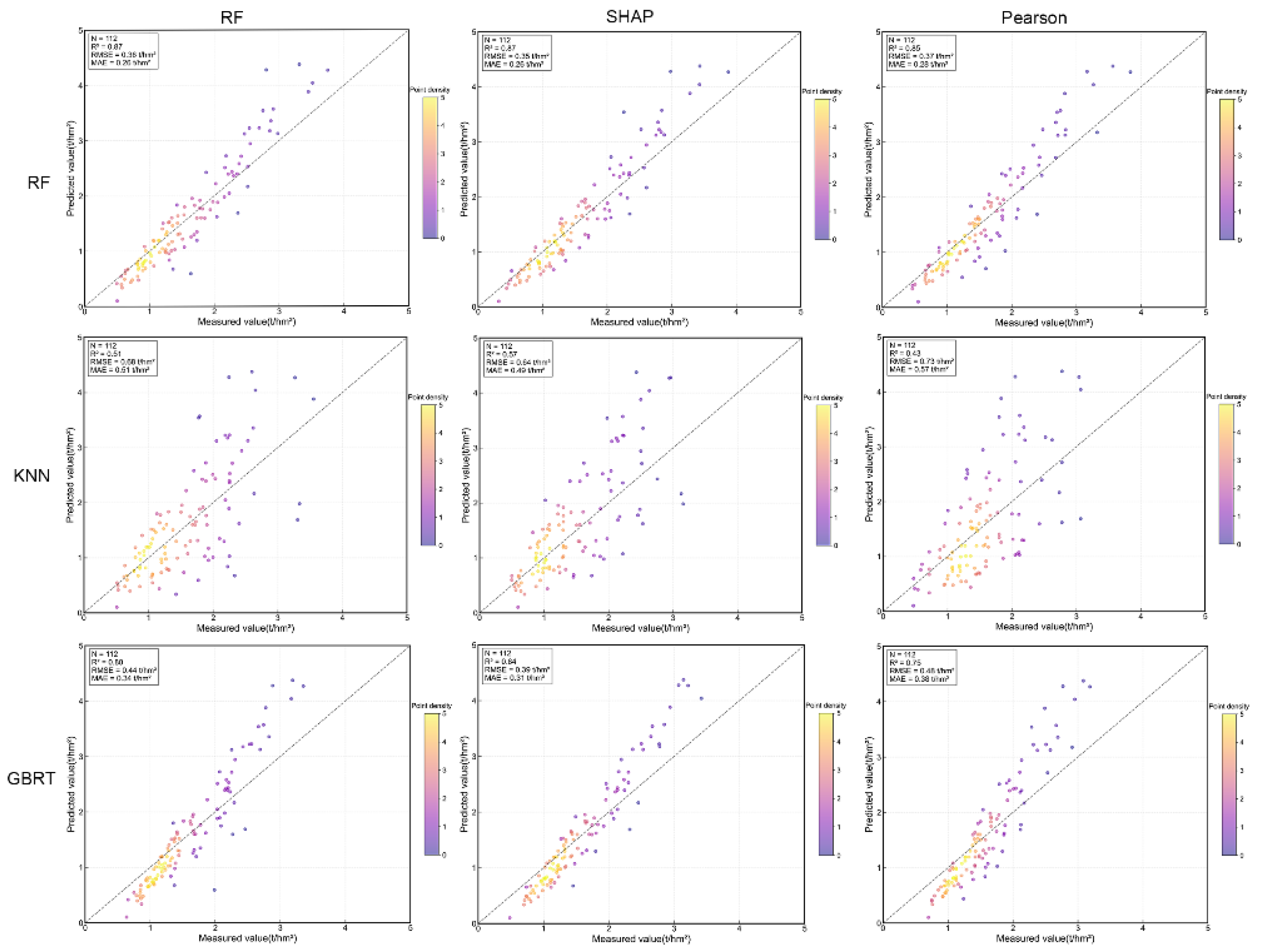
Figure 7.
Comparison of the accuracy of various models after GP feature optimization: In the horizontal direction, the three models are RF, KNN, and GBRT, and the three groups of feature variables are Pearson, RF, and SHAP. In the vertical direction, the three groups of feature variables are Pearson, RF, and SHAP, and the three models are RF, KNN, and GBRT.
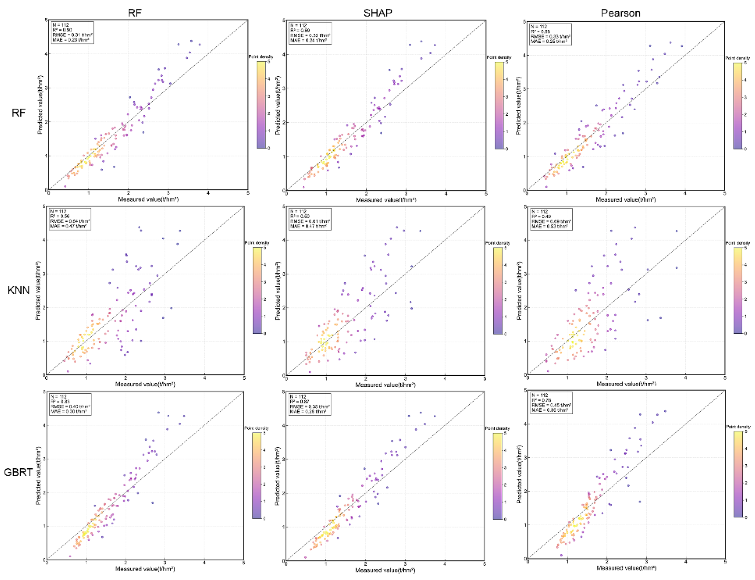
Figure 8.
Comparison of predicted values and true values of the RF model after GP optimization.
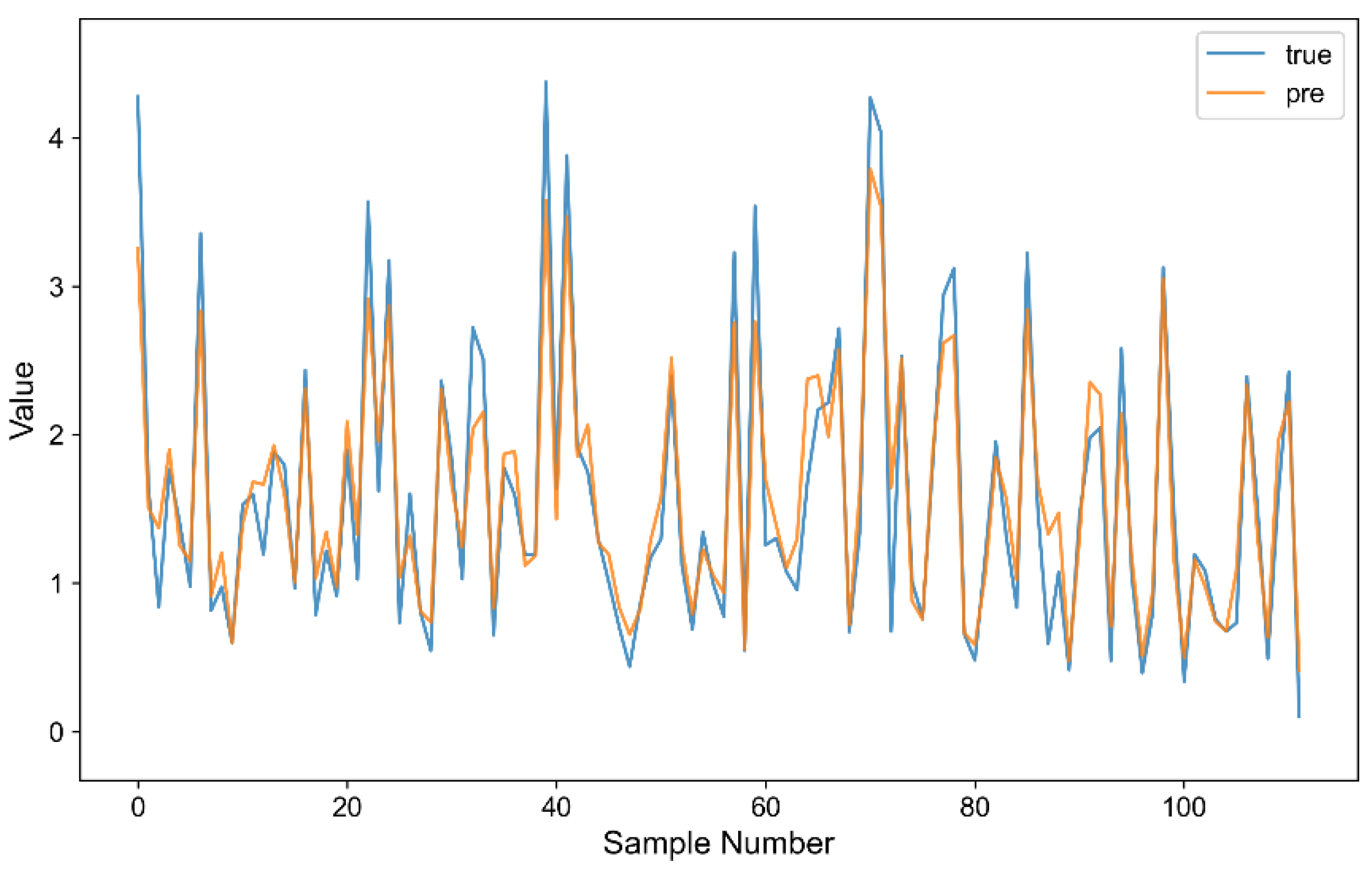
Figure 9.
Spatial pattern of AGB in grasslands within the Three Parallel Rivers Area.
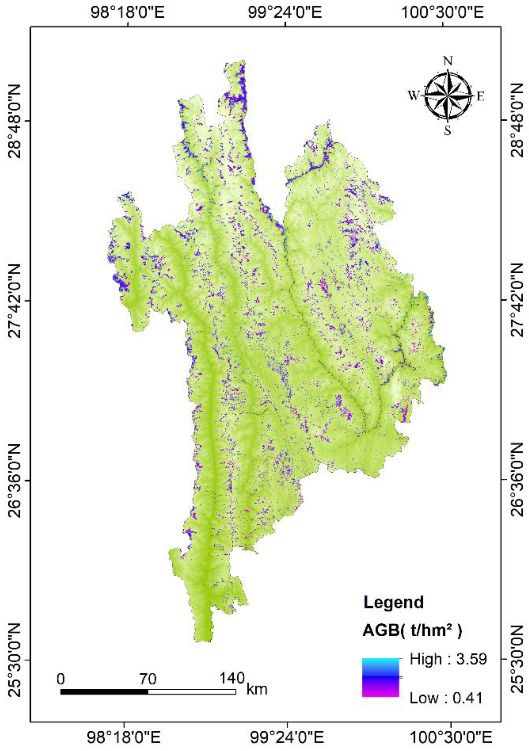

Table 1.
Statistical analysis of biomass in the sample plots.
| Number of Samples | Minimum Value | Maximum Value | Mean Value | Standard Deviation | Variance |
|---|---|---|---|---|---|
| 112 | 0.10 | 4.38 | 1.57 | 0.97 | 0.95 |
Table 2.
Formula for calculating texture features.
| Name | Formula |
|---|---|
| Mean | |
| Variance | |
| Homogeneity | |
| Dissimilarity | |
| Entropy | |
| Contrast | |
| Second Moment | |
| Correlation |
* i and j denote the row and column indices of the GLCM, Fi, j denotes the values of the elements in the normalized covariance matrix after normalization of the ith row and jth column, and µi, j denotes the mean value of the GLCM.
Table 3.
Calculation Formula of Vegetation Index.
| Name | Formula |
|---|---|
| NDVI | |
| GNDVI | |
| RVI | |
| EVI | |
| DVI | |
| SAVI | |
| MSAVI | |
| OSAVI |
* B2, B3, B4, and B8 respectively represent the blue light, green light, red light, and near-infrared bands of the Sentinel-2 satellite.
Table 4.
Modeling results of each model after GP optimization.
| Model | Feature Selection Methods | R² | RMSE | MAE |
|---|---|---|---|---|
| RF | Pearson | 0.88 | 0.33 | 0.25 |
| RF | 0.90 | 0.31 | 0.23 | |
| SHAP | 0.89 | 0.32 | 0.24 | |
| KNN | Pearson | 0.49 | 0.70 | 0.53 |
| RF | 0.56 | 0.64 | 0.47 | |
| SHAP | 0.60 | 0.61 | 0.47 | |
| GBRT | Pearson | 0.78 | 0.46 | 0.36 |
| RF | 0.83 | 0.40 | 0.30 | |
| SHAP | 0.87 | 0.35 | 0.28 |
Disclaimer/Publisher’s Note: The statements, opinions and data contained in all publications are solely those of the individual author(s) and contributor(s) and not of MDPI and/or the editor(s). MDPI and/or the editor(s) disclaim responsibility for any injury to people or property resulting from any ideas, methods, instructions or products referred to in the content. |
© 2025 by the authors. Licensee MDPI, Basel, Switzerland. This article is an open access article distributed under the terms and conditions of the Creative Commons Attribution (CC BY) license (http://creativecommons.org/licenses/by/4.0/).
Copyright: This open access article is published under a Creative Commons CC BY 4.0 license, which permit the free download, distribution, and reuse, provided that the author and preprint are cited in any reuse.


