Submitted:
22 July 2025
Posted:
23 July 2025
You are already at the latest version
Abstract
Synthetic aperture radar (SAR) is one of the few instruments capable of providing high-resolution global two-dimensional (2D) measurements of ocean waves. Since 2014 and then 2016, the Sentinel-1A/B satellites, whenever operating in a specific Wave mode (WV), have been providing ocean swell spectrum data as Level-2 (L2) OCeaN products (OCN), derived through a quasi-linear inversion process. This WM acquires small SAR images of 20x20km footprints alternating between two sub-beams: WV1 and WV2, with a incidence angles of approximately 23° and 36° respectively, to capture ocean surface dynamics. The SAR imaging process is influenced by various modulations, including hydrodynamic, tilt, and velocity bunching. While hydrodynamic and tilt modulations can be approximated as linear processes, velocity bunching introduces significant distortion due to the satellite’s relative motion with respect to the ocean surface and lead to constructive or destructive effects on the wave imaging process . Due to the associated azimuth cut-off, the quasi-linear inversion primarily detects ocean swells with wavelengths longer than 200 meters, limiting the resolution of smaller-scale wave features. The 2D spectral partitioning technique used in the Sentinel-1 WV OCN product separates different swell systems, known as partitions, based on their frequency, directional and spectral characteristics. The accuracy of these partitions can be affected by several factors, including non-linear effects, large-scale surface features, and the relative direction of the swell peak to the satellite’s flight path. To address these challenges, this study proposes a novel quality control framework using a Machine Learning (ML) approach to develop a Quality Flag (QF) parameter associated with each swell partition provided in the OCN products. By pairing collocated data from Sentinel-1 (S1) and WaveWatch III (WW3) partitions, the QF parameter assigns each SAR-derived swell partition one of five quality levels: “very good,” “good,” “medium,” “low,” or “poor”. This ML-based method enhances the accuracy of wave partitions, especially in cases where non-linear effects or large-scale oceanic features distort the data. The proposed algorithm provides a robust tool for filtering out problematic partitions, improving the overall quality of ocean wave measurements obtained from SAR. Moreover, the variability in the accuracy of swell partitions, depending on the swell direction relative to the satellite’s flight path, is effectively addressed, enabling more reliable data for oceanographic studies. This work contributes to a better understanding of ocean swell dynamics derived from SAR observations and supports the numerical swell modeling community by aiding in the refinement of models and their integration into operational systems, thereby advancing both theoretical and practical aspects of ocean wave forecasting.
Keywords:
sentinel-1 mission
; SAR
; wave spectrum
; partitioning
; quality flag
; machine learning
; remote sensing
1. Introduction
Copernicus, the Earth observation component of the European Union’s Space program, plays a pivotal role in monitoring our planet and its environment for the benefit of European citizens [33]. Within this program, the S1 mission, operated by the European Space Agency (ESA), is equipped with SAR satellites. The S1 satellites, which use C-band SAR (central frequency 5.405 GHz), are capable of collecting data across multiple acquisition modes, with WV predominantly employing vertical-vertical polarization (VV) to observe open ocean conditions [35]. The launch of Sentinel-1A occurred on April 3, 2014, followed by Sentinel-1B on April 25, 2016. Both satellites operated in the same orbital plane with a phase shift of 180°. Sentinel-1B stopped delivering data in December 23, 2021, was decommissioned in 2023 and replaced by Sentinel-1C (launched in December 5, 2024). The data obtained by Sentinel-1 in WM are routinely processed into L2 OCN products and include directional ocean wave spectra generated using a quasi-linear inversion method [17]. This inversion process provides valuable information on the distribution of wave variance in frequency and direction. However, SAR-based inversion is mainly applicable to long ocean swells (with wavelengths greater than 200 m) [1,5,8] and to wave propagation in the marginal ice zone [3,25].
Although integral parameters from SAR-derived spectra can effectively characterize a single-swell system, they become less informative when multiple, overlapping wave systems are present (Figure 1). In such cases, it becomes essential to partition the ocean wave spectrum into independent wave systems to ensure accurate data analysis and quality control. Within the L2 OCN product, the ocean wave spectrum is divided into a maximum number of five distinct partitions [17] using the "watershed" algorithm, originally introduced by [4,13]. Each partition is described by its corresponding integral parameters, including the partitioned Significant Wave Height (Hs), the peak wavelength, and peak wave direction (Figure 1).
A direct comparison between the SAR-derived wave partitions and those obtained from the WW3 model [28] reveals discrepancies, particularly between the dominant and secondary swell systems. Differences in partitioned wavelengths exhibit positive clustering in the azimuth direction and negative clustering in the range direction [18,29,31]. Notably, a study by [15] in the Australian region shows Root-Mean-Square Errors () of 0.70 m for Hs, 0.9 s for mean periods, and 30° for wave direction. These discrepancies are largely attributed to the motion of ocean waves with radial velocity components, which induce Doppler frequency shifts in radar echoes. As a result, SAR image points with radial velocity components are displaced along the azimuth direction, leading to non-linear effects when converting SAR data into ocean wave spectra. To address these challenges, ML techniques are commonly employed to handle such non-linearities. While existing methods have corrected some integrated SAR wave parameters (e.g., total Hs, as discussed by [21]), they have yet to correct individual ocean wave systems.
This study applies data-driven ML techniques to define a prior QF for each of the five wave partitions derived from Sentinel-1 WV OCN products. The QF is determined by learning partition error parameters, including relative errors in partitioned significant wave height (),
the relative error of the peak period (),
and the absolute error of the peak wave direction (),
based on collocated SAR and WW3 partition pairs. By transitioning from absolute to relative errors, this data-driven approach ensures a more balanced distribution of integral parameters across the QF classes. This adjustment mitigates the disproportionate influence of higher values on error estimation, thereby reducing bias and providing a more equitable representation of partition quality.
The primary contributions of this research are: (1) the application of ML algorithms to improve the qualification of S1 ocean wave spectrum partitioning, (2) an explanation of the model’s predictions and how they relate to the geophysical inversion process using SAR data, and (3) the establishment of a framework for future research aimed at advancing the retrieval of ocean wave spectra from SAR.
The manuscript is structured as follows: Section 2 presents the dataset utilized in this study. Section 3 outlines the full ML methodology used. In Section 4, we present the results and validate the model. Section 5 offers an in-depth discussion of the findings, and Section 6 concludes the paper with future research perspectives.
2. Data Set Collection
2.1. Sentinel-1 WV OCN OSW Products
The S1A/B WV mode operates by acquiring SAR images, or imagettes, spaced 100 km apart, with two alternating incidence angles, WV1 and WV2, along the satellite’s flight path using a "leap frog" acquisition strategy [24]. In each acquisition, the S1 WV mode can only operate in a single polarization, VV or HH, with VV polarization being the default for global ocean observations. Each acquired imagette covers an area of approximately 20 x 20 km, with a high spatial resolution of 5 meters. The ocean wave spectrum (OSW) component of the WV OCN product is derived from Level-1 (L1) Single Look Complex (SLC) SAR imagettes, processed through the ESA L2 spectral inversion unit [17].
The inversion process begins with the estimation and removal of non-linear contributions from the SAR data, which is essential for improving the accuracy of the final results. Once the non-linearity is treated, the cross-spectra technique is applied to resolve the 180° directional ambiguity in wave propagation, which is crucial for obtaining reliable directional information. This method allows the retrieval of the ocean wave spectrum with a directional resolution of 10° and 30 exponentially spaced wave numbers, spanning from 30 to 800 meters. The final step of the process involves partitioning the 2D ocean wave spectrum into five independent ocean wave systems using the watershed algorithm, after which the integral parameters (such as Significant Wave Height, peak wavelength, and peak wave direction) for each partition are computed.
For the purposes of this study, we use data acquired exclusively from the S1A satellite, covering both WV1 and WV2 modes with VV polarization, collected between December 2024 and February 2025. This time period was selected because it corresponds to the deployment of version 3.90 of the S1 L2 Instrument Processing Facility (IPF), which includes a new SAR Modulation Transfer Function (MTF) tuning. This upgrade significantly improves wave inversion performance from SAR imagery [17].
Additionally, to ensure the integrity of the ocean wave data, products acquired at latitudes above 55° North and South are filtered out to exclude any possible contamination from sea ice, which could distort wave measurements.
The publicly available S1 OCN WV data used in this study can be accessed through the Copernicus Open Access Hub [34].
2.2. WW3 Hindcasts
The WW3 Hindcast, part of the Integrated Ocean Waves for Geophysical and other Applications (IOWAGA) project led by IFREMER, is a third-generation wave model that resolves the spectral action density equilibrium equation for wavenumber-directional spectra. It is driven by data on 3-hour wind and ice concentration from the European Center for Medium-Range Weather Forecasts (ECMWF) product [2,22]. The model operates with spatial and temporal resolutions of 0.5° and 3 hours, respectively. The spectral data are organized into 32 frequency bins, exponentially spaced from 0.038 to 0.7159 Hz, and 24 directional bins, each separated by 15°. To partition the wave spectra, the model employs the “watershed” algorithm, which divides the spectra into five partitions corresponding to different swells, as well as one partition for wind seas. Wind seas are represented by Partition 0, while Partitions 1 through 5 correspond to various swell systems. The accuracy of the model’s wave parameter has been validated against buoy and altimeter measurements, showing strong agreement [2,9,23]. The WW3 Hindcast data is available for download through the IFREMER FTP server (ftp://ftp.ifremer.fr/ifremer/ww3/HINDCAST/).
2.3. Match-Up Partitions
The S1 OCN WV OSW products were collocated with the WW3 hindcasts based on the closest spatial and temporal grid points, within a window of 0.25° in latitude/longitude and 1.5 hours in time. To ensure the best matchups at the partitioned swell level, these spatio-temporal collocations were further refined by identifying the closest partition matches. For this partition cross-assignment, the spectral distance between the partitions was defined, as proposed by [14], according to the following equation:
In this equation, and represent the peak propagation direction and peak period of each swell system, respectively. The constant r was set to 250, which scales the period error appropriately: a 20° directional error is treated as equivalent to an 8% error in wave period, reflecting the typical SAR swell measurement accuracy. Additionally, the value of was chosen to define the error thresholds to ensure 30° directional error and a 12% in period error to give a spectral distance equal to one [30].
No further filtering was applied to the dataset to preserve a comprehensive representation of the various errors inherent in the inversion and partitioning processes, as well as any non-geophysical contributions present at the ocean surface.
3. Method Details
3.1. Quality Flag Definition
The Normalized Radar Cross-Section (NRCS) is influenced by several error sources, including geometric distortions, sensor-specific acquisition errors, and the presence of non-geophysical factors such as atmospheric influences and surface roughness at the air-sea interface. Additionally, the quasi-linear inversion process employed to derive ocean wave spectra from SAR data introduces further inaccuracies. The partitioning algorithm, which divides the ocean wave spectrum into distinct wave systems, is also subject to its own set of errors. To address these complexities, the first critical step in our algorithmic approach is to independently quantify the errors in , , and at the partition level with respect to the WW3 model data.
These errors are estimated using a supervised ML algorithm, which leverages a set of SAR-derived observables (i.e., features) to predict discrepancies in the ocean wave parameters [7]. The features used for the error estimation process are detailed in Table 1. The computation of some features is described in detail in [17].
Regardless of the acquisition mode (WV1 or WV2), the same set of features is used to estimate the three primary errors. This necessitates the training of six separate models tailored to the S1A mission, each aimed at improving the accuracy of partition-level error quantification and ultimately refining the ocean wave parameter retrieval process.
The second step of the algorithm focuses on computing a combined error metric for each individual acquisition mode (i.e., WV1 and WV2). This combined error, denoted as and defined in Eq. 6, is calculated by multiplying the three primary error estimates—, , and —previously inferred using the trained models applied to the validation dataset, which consists of all S1A acquisitions from February 2025. The metric is expressed as:
Since the ultimate goal is to assess the quality of ocean swell systems in a manner that is independent of the SAR acquisition mode, a unified combined error metric is produced by merging the mode-specific error estimates from both WV1 and WV2. This approach is motivated by the need for consistent and homogeneous error characterization across different SAR configurations. Since both WV1 and WV2 data are used interchangeably in operational wave monitoring and analysis, having a mode-agnostic quality metric ensures comparability between partitions retrieved under different acquisition conditions. By assembling the combined error from both modes, we enable a seamless interpretation of partition-level quality, facilitating the identification and classification of ocean swell systems without bias introduced by the acquisition geometry.
This reference error is then partitioned into five equally probable intervals using the q-quintile method, commonly referred to as Quintile. These intervals represent distinct levels of error severity, ranging from low to high. Once this reference error distribution is established, the calculated for each partition is matched to the corresponding quintile range. Based on this comparison, each partition is assigned a quality label: “Very Good,” “Good,” “Medium,” “Low,” or “Poor.” This classification serves as an indication of the reliability and accuracy of the partition, facilitating informed decision-making in further analyses.
3.2. Machine Learning Data Set
In the context of algorithm development, we focused on the S1 WV OCN dataset, which was acquired over two months : December 2024 and January 2025. These data were assigned to the training phase, with an 80%-20% split for training and validation, respectively. This approach ensures that the model is rigorously tested on unseen data during training. Data from February 2025 were used exclusively for model evaluation, providing an independent test set to assess the model’s generalizing ability.
During the training process, no data normalization was performed, as the chosen machine learning algorithm is inherently robust to raw, unnormalized data, facilitating direct input handling without additional preprocessing steps and data transformation.
The targets for the machine learning models are : , , and . We selected the absolute error to emphasize the overall discrepancy between WW3 and the SAR observations, rather than focusing on the signed difference. Given that the WW3 does not account for all geophysical complexities, we place greater trust in the observational data as a more reliable reference, thereby enhancing the confidence in the results.
3.3. Machine Learning Modeling
In this study, we initially used a traditional Random Forest algorithm; however, it soon revealed limitations in terms of interpretability. Consequently, we shifted our focus to the eXtreme Gradient Boosting (XGBoost) supervised learning algorithm, which offered improved performance and explainability. XGBoost is a scalable, distributed machine learning library based on gradient-boosted decision trees (GBDT). A decision tree is a model that makes decisions by splitting data into branches based on simple conditions, forming a set of "true or false" statements. Since its debut in 2014, XGBoost has become one of the most widely adopted algorithms among data scientists and machine learning practitioners due to its high performance, particularly for structured data problems. The library is open-source [32] and is able to efficiently train and test models on large datasets.
One of the primary reasons for selecting XGBoost in our study is its regularization capabilities. Regularization helps to control overfitting, where the model fits too closely to the training data, thereby reducing its ability to generalize to unseen data. XGBoost applies L1 and L2 penalties to the weights and biases of each tree, helping to maintain model simplicity and prevent overfitting. Additionally, XGBoost is highly optimized, with features that make it more memory efficient, such as cache-awareness, which is crucial when working with large datasets.
XGBoost also stands out for its ability to handle missing data, eliminating the need for imputation, and its ability to work with data in their raw, unnormalized state, simplifying the preprocessing process. These advantages make XGBoost an attractive choice for dealing with complex data problems.
To fine-tune the XGBoost model and achieve optimal performance, hyperparameter tuning was performed. Hyperparameters are critical settings that influence how the model learns, and selecting the right ones can significantly improve model accuracy. Given the large number of hyperparameters, finding the best combination manually is impractical. Therefore, we used the GridSearch technique [19] to systematically explore different combinations of hyperparameters. In this process, multiple sets of hyperparameters are tested within a defined search space, and the performance of the model is evaluated on a validation dataset. Although this method is effective, it can be computationally expensive, particularly as the number of parameters and their possible values increases. A list of the hyperparameters most commonly tuned in XGBoost is provided in Table 2, with additional parameters available in [32].
Machine learning models must exhibit robustness, meaning they should minimize the impact of outliers and prioritize the influence of typical data points. In tasks such as parameter estimation, using a robust loss function (e.g., absolute error) is often preferred over a non-robust one (e.g., squared error) because it is less sensitive to large deviations. Common loss functions in regression tasks are squared loss, , and absolute loss, . While squared loss is highly sensitive to outliers, making it less reliable in such cases, absolute loss is more resilient as it focuses on the order of data rather than their absolute magnitude [20].
To leverage the advantages of both, the pseudo-Huber [6,10] loss function is often used. This hybrid function blends the properties of both quadratic and absolute loss while maintaining the smooth differentiability required for optimization. It is mathematically expressed as:
where is the threshold parameter that controls the transition between the quadratic and linear behavior of the loss.
For small values of x, the pseudo-Huber loss behaves like a quadratic function,
while for large values of x, it approximates the absolute loss,
In XGBoost, the model is optimized using gradient-based methods, such as gradient descent, to minimize the chosen loss function while incorporating regularization to prevent overfitting. The model’s objective function combines the loss function and a regularization term, as shown in Eq. 8:
Here, l represents the loss function (e.g., pseudo-Huber), denotes the prediction from the t-th tree, and is the regularization term that helps avoid overfitting by penalizing overly complex models. The gradient descent process iteratively updates the model parameters to minimize this objective. Additional details on regularization can be found in [7].
4. Results
4.1. Metrics Definition
Model training was conducted using an 8GB NVIDIA RTX A2000 graphics card. Thanks to XGBoost’s ability to leverage parallel processing, the grid search and model training time for each model was approximately three hours. The performance of the XGBoost models in predicting the errors in S1 ocean wave spectrum partitioning parameters and controlling the final partitioning labeling was assessed using several evaluation metrics. These metrics include the , Normalized Root Mean Squared Error (), standard deviation (), Median Absolute Error (), Scatter Index (), coefficient of determination (), and explained variance score ().
The is a widely used metric that measures the square root of the average of squared differences between predicted and observed values. It is sensitive to large errors, thus providing a strong indication of how far off the predictions are from the actual values. The RMSE is defined as:
where is the predicted value obtained with the model, and is the true value.
The NRMSE is a normalized version of the RMSE that scales the error by the range or the mean of the observed values. This allows for a comparison of error across different datasets with different ranges or units. It is calculated as:
The STD measures the amount of variation or dispersion of a set of values. In the context of model evaluation, it is useful for understanding the variability in the errors and is given by:
where is the mean of .
The MAE measures the median of the absolute differences between the predicted and true values, making it a robust metric to outliers, as it gives equal weight to each error regardless of magnitude. The MAE is defined as:
The SI is a metric used to assess the consistency of the model’s predictions by calculating the ratio of the RMSE to the mean of the observed values. It provides insight into the relative error of the predictions, and is given by:
The R² is a statistical measure that indicates how well the predicted values match the actual values. It measures the proportion of the variance in the dependent variable that is predictable from the independent variables. An R² value of 1 means perfect predictions, while a value of 0 indicates no correlation between predicted and actual values. R² is computed as:
The EVS is similar to R² but with the key difference that it does not penalize for systematic offsets in the predictions. It measures the proportion of variance in the target variable that is explained by the model, and is defined as:
4.2. Overall Models Performances
The results for the two acquisition modes, categorized by partition class (i.e., quality flag), are derived from the validation dataset using the partition-effective Hs, peak wavelength, and peak wave direction with respect to WW3, and are presented in Table 3, Table 4, and Table 5, respectively. This analysis provides a clear view of how the model distinguishes between good and bad partitions.
Performance metrics for each class, evaluated based on partition parameters and compared to the WW3 model, reveal insightful trends. For each parameter, the model demonstrates strong initial agreement with WW3. Specifically, for the ’very good’ class, the agreement is excellent, with an R² value of 0.77 (overall mean). However, as the class quality decreases towards ’poor,’ the agreement progressively weakens. In the ’poorest’ class, the distributions of SAR and WW3 diverge significantly, reflecting a clear mismatch between the two. This trend holds true for almost the entire range of partition wave parameters.
For the subsequent analysis, we will focus exclusively on the extreme classes—"very good" and "poor"—along with the "medium" class, as these categories represent the most relevant distinctions in partition quality for our purposes.
To showcase the robustness of the methodology in partition classification, from high-quality (Very Good) to low-quality (Poor) classes for both WV1 and WV2 across partition parameter ranges, scatter plots are presented in Figure 2 for the case of Hs. In addition to the clear class separation, the plots reveal a consistent trend of increasing error as partition quality declines, with a notable mismatch in the Poor class. This mismatch underscores the model’s ability to effectively capture variations in error distribution, reinforcing the reliability of the classification approach. These findings highlight the model’s strength in preserving accuracy across diverse data quality levels, even under challenging conditions. Further partition parameters, including peak wavelength and peak wave direction, are detailed in Appendix A and Appendix B.
4.3. Focused Analysis of Partition Classification Performance
The class distribution, depicted in Figure 3, demonstrates a consistent and largely homogeneous spread across all partitions, showing no significant bias towards any particular class. This indicates an overall well-balanced distribution.
While the class distribution remains balanced for both ascending and descending passes, a slight difference is noticeable in the medium and low classes when comparing the two modes. This discrepancy likely stems from combining the errors between these modes, which can shift the percentile limits compared to maintaining separate percentiles for each.
A closer inspection of Figure 4 reveals how the algorithm assigns quality classifications across the different wave partitions. The first partition—corresponding to the main swell—is consistently identified as the most significant and is predominantly labeled as "very good" or "good." This outcome aligns well with expectations, as the algorithm is designed to better identify the most relevant wave state information from the SAR data.
The classification of the second partition, typically associated with a secondary swell, exhibits a more uniform distribution across quality categories. This pattern is particularly evident in WV1 data, where it remains largely independent of satellite heading. In contrast, for WV2, the behavior of the second partition is slightly different, which could be attributed to the combined uncertainty introduced by merging the classification thresholds from the two acquisition modes.
The algorithm tends to classify these lower-ranked partitions as "low" or "poor" simply because they are less relevant from a geophysical perspective. This results in a clear distinction in partition quality, which can be especially useful for end users of SAR wave data when interpreting the most meaningful components of the sea state.
To further evaluate the performance of the quality classification, we examine the spatial distribution of quality classes ("Very Good," "Medium," and "Poor") across both WV1 and WV2 modes (Figure 5). These maps show spatial variations that appear broadly consistent between the two modes, suggesting that the classification patterns are more closely related to the underlying algorithmic process than to differences in acquisition mode.
Some of these spatial trends can be partially explained by the varying frequency of WV acquisitions across regions. For instance, the coverage near Europe is limited due to the use of alternative Sentinel-1 acquisition modes: Interferometric Wide Swath (IW) mode is primarily employed for land monitoring over the mainland, while Extra Wide Swath (EW) mode is more commonly used in areas such as the Azores. This results in a lower number of WV observations available for quality assessment in those zones.
A more detailed examination of the spatial distribution of quality classes highlights certain regional tendencies:
- Very Good: This class tends to be more frequent in mid-latitude. In contrast, it is less commonly observed in the northern Indian Ocean and in coastal regions, where environmental factors such as monsoon activity, coastal topography, and proximity to land can affect the quality of wave retrievals.
- Medium: This class is relatively evenly distributed across the globe, with increased presence in transitional zones near the equator and subpolar regions. These areas are characterized by more variable conditions that often result in intermediate-quality inversions.
- Poor: This class is more frequently observed at high latitudes in both hemispheres, where strong and variable wind speeds, along with complex atmospheric phenomena, can negatively impact SAR wave retrieval. Additionally, some chaotic offshore regions experience increased maritime traffic and environmental variability, which may introduce biases in the sea state inversion process. These factors contribute to lower quality classifications in these areas.
These spatial patterns provide end users of SAR wave data with clearer guidance on the expected quality of sea-state information, supporting a more informed use of the products in different geographic contexts.
5. Discussion
Accurately deriving ocean wave parameters from SAR data is inherently complex, influenced by both radar system limitations and environmental factors. A critical component in this process is the MTF, which defines how spatial frequencies in the SAR cross-spectrum are translated into the ocean wave spectrum. The MTF is particularly sensitive to wave motion along the radar’s range axis, whether moving toward or away from the radar. This motion introduces a Doppler effect that affects the radar backscatter signal and, consequently, the retrieval of the wave spectrum. These Doppler-induced shifts, combined with the inherent limitations of the MTF, add complexity in accurately interpreting SAR data for ocean wave analysis (Figure 6).
In addition to MTF-related challenges, environmental phenomena such as rainfall and other atmospheric or oceanic features further impact the NRCS, affecting wave retrieval. Rainfall, (Figure 7), can influence the NRCS by altering the surface roughness, potentially masking the geophysical signal. Oceanic fronts, characterized by sharp gradients in sea surface temperature and salinity, and atmospheric fronts (Figure 8), marked by strong near-surface wind variations, also introduce discontinuities in the NRCS, further complicating wave spectrum retrieval.
To go deeper into model explanation and interpretability, an illustrative example of Model interpretation using SHAP-based explanations (Figure 7 )is provided for estimating the errors in the three partition-integral parameters for the WV1 acquisition (see Figure 9, Figure 10, and Figure 11). The explanation for the WV2 acquisition is essentially the same and is therefore not shown. Each plot investiagtion holds two type of analysis one for the model expalanation : this explanation helps interpret the importance of each feature (Table 1) and how they affect the model’s predictions. A second plot based on features importance introduce the concept of feature clustering to help visualize redundancy among features. This clustering aims to group features that provide similar information to the model. This means that a model might be able to use either of two related features and achieve similar predictive performance. Traditional methods like correlation matrices can identify such relationships. In the context of SHAP’s feature clustering, "distance" between features is typically scaled between 0 and 1, where a distance of 0 means the features are perfectly redundant, and a distance of 1 means they are completely independent. In our case, we set the clustering cutoff at 0.5 : the bar plot will only show clusters (or groups) of features that have a clustering distance less than 0.5. This means only highly redundant features (those sharing more than 50% of their explanation power) will be visually grouped together. Less redundant features, even if they have some relationship, will be displayed individually.
The most impactful predictors for the prediction (as depicted in Figure 9 (a)) are the effective partition and the normalized variance of the SLC imagette. These features are physically meaningful, as they directly relate to wave energy and sea surface texture, and their influence is clearly reflected in the model’s behavior. Specifically, the model tends to associate higher effective values with lower predicted error, leading to a higher quality classification for those partitions. Conversely, lower values are typically linked to higher predicted errors and lower quality assessments. This indicates that the model prioritizes energetic sea states, while treating weaker partitions more conservatively.
A further insight comes from the feature clustering (Figure 9 (b)): statistical moments derived from the SLC imagette—namely skewness, kurtosis, and normalized variance—form a single cluster, indicating they collectively explain a significant portion (over 50%) of the model’s behavior. Another correlated group includes peak wave parameters such as peak direction and peak period. Most other features appear relatively independent in their contribution to predicting , suggesting the model relies on a focused subset of physically meaningful indicators to make its predictions.
In the context of peak period error estimation (Figure 10 (a)), the predominant determinant of model fidelity is the energy ratio between the partition’s spectral peak and the maximum energy boundary. A diminished energy ratio corresponds to an escalation in relative error, underscoring its critical influence on the model’s uncertainty quantification. Conversely, elevated energy ratios are associated with reduced error magnitudes, indicative of enhanced precision in the peak period retrieval.
Consistent with the model’s objective, the peak period itself constitutes the secondary most salient feature impacting error prediction. Its influence manifests nonlinearly and is modulated by the swell propagation direction relative to the SAR azimuth, as well as hydrodynamic effects and tilt modulation intrinsic to the SAR wave retrieval mechanism.
In particular, while the partition index has a limited influence on the estimation of , the model leverages the partition rank (i.e., the "p" feature) more substantially when predicting . This suggests that the model attempts to refine its error estimation by accounting for the sequential ordering of swell systems, which aligns with the earlier observations regarding the distribution of quality classes across partition ranks. Such a strategy reflects the model’s recognition of the varying relevance and complexity of each partition in accurately retrieving peak period information.
Furthermore, we observe a similar behavior to in terms of feature redundancy (Figure 10 - (b)): the SLC imagette statistics are often redundant, leading the model to group them together. This redundancy extends to some other peak partition parameters computed in different geometries, which also appear to be redundant for the model.
The analysis of partition wave direction error (Figure 11 (a)) reveals a pronounced sensitivity to the alignment between the dominant wave direction and the satellite heading. This confirms the fundamental influence of wave propagation dynamics relative to the SAR flight azimuth, which imposes intrinsic constraints on the inversion accuracy, as previously outlined. The elevated importance of the ambiguity factor—ranked third among predictors—further highlights its critical role in modulating directional uncertainty, distinguishing this error metric from others.
Consistent with patterns observed in the estimation of other wave parameters, the energy ratio once again proves to be a principal driver, ranking as the second most impactful feature. The peak wave direction also contributes meaningfully, occupying the sixth position in the feature importance hierarchy, emphasizing its relevance in capturing directional variability.
Apart from the correlated statistical features derived from the SLC imagette (Figure 11 (b)), the model does not identify additional significant feature groupings influencing . This suggests that directional error arises from a more discrete set of physical and retrieval factors, underscoring the complex interplay between wave dynamics and SAR observation geometry. These insights pave the way for targeted improvements in SAR wave inversion methodologies, with the potential to enhance directional retrieval fidelity under challenging environmental conditions.
6. Conclusions
This study presents a novel approach to improving the reliability of SAR-based ocean wave retrieval through an advanced partition classification algorithm. By leveraging machine learning and explainability techniques, the method effectively addresses challenges that have long hindered the accuracy of wave spectrum interpretation—particularly those arising from system-induced distortions such as azimuth cutoff effects and the modulation transfer function.
What sets this work apart is not just the classification accuracy, but the intelligent selection of physically meaningful features that align with the behavior of ocean waves. This synergy between data-driven modeling and geophysical understanding enables a deeper insight into SAR performance under varying sea conditions. The model’s capacity to isolate the most trustworthy partitions creates opportunities for more targeted and confident use of SAR data in both scientific research and operational settings.
Beyond the technical contributions, the integration of interpretability adds a valuable layer of transparency. Rather than treating the algorithm as a black box, the use of SHAP-based analysis illuminates the factors influencing each decision, allowing users to validate outcomes and potentially refine the input data or retrieval strategies.
In a broader sense, this work contributes to a growing effort in Earth observation to make remote sensing tools not only more accurate but also more accountable and accessible. The proposed method offers a foundation upon which future SAR-based systems can be built—systems that are capable of adapting to complex marine environments while providing clear, interpretable results. As ocean monitoring becomes increasingly vital in the context of climate change and maritime activity, such tools will be essential for both research and real-world applications.
Author Contributions
Conceptualization, data curation, writing–original draft preparation, Amine Benchaabane; methodology, Romain Husson; supervision, Romain Husson; software, Amine Benchaabane; funding acquisition, Muriel Pinheiro, writing–review and editing, Guillaume Hajduch, All authors have read and agreed to the published version of the manuscript.
Funding
Not applicable
Institutional Review Board Statement
Not applicable
Informed Consent Statement
Written informed consent has been obtained from the patient(s) to publish this paper
Data Availability Statement
Data will be made available on request.
Acknowledgments
The results presented here are outcome of the ESA contract Sentinel-1 / SAR Mission Performance Cluster Service 4000135998/21/I BG. Copernicus Sentinel-1 mission is funded by the EU and ESA. The views expressed herein can in no way be taken to reflect the official opinion of the European Space Agency or the European Union.
Conflicts of Interest
The authors declare that they have no known competing financial interests or personal relationships that could have appeared to influence the work reported in this paper.
Abbreviations
The following abbreviations are used in this manuscript :
| ESA | European Space Agency |
| IPF | Instrument Processing Facility |
| ML | Machine Learning |
| MPC | Mission Performance Cluster |
| MTF | Modulation Transfer Function |
| NRCS | Normalized Radar Cross Section |
| OCN | Level 2 OCeaN product |
| OSW | Ocean SWell |
| QF | Quality Flag |
| SAR | Synthetic Aperture Radar |
| S1 | Sentinel-1 mission |
| VV | Vertical transmit and Vertical received polarization |
| WV | WaVe mode |
| WV1 | Wave mode 1 beam |
| WV2 | Wave mode 2 beam |
| WW3 | Wave Watch 3 |
| XGBoost | eXtreme Gradient Boosting |
Appendix A. Partitions Classification Performed on Peak Wave Direction
Figure A1.
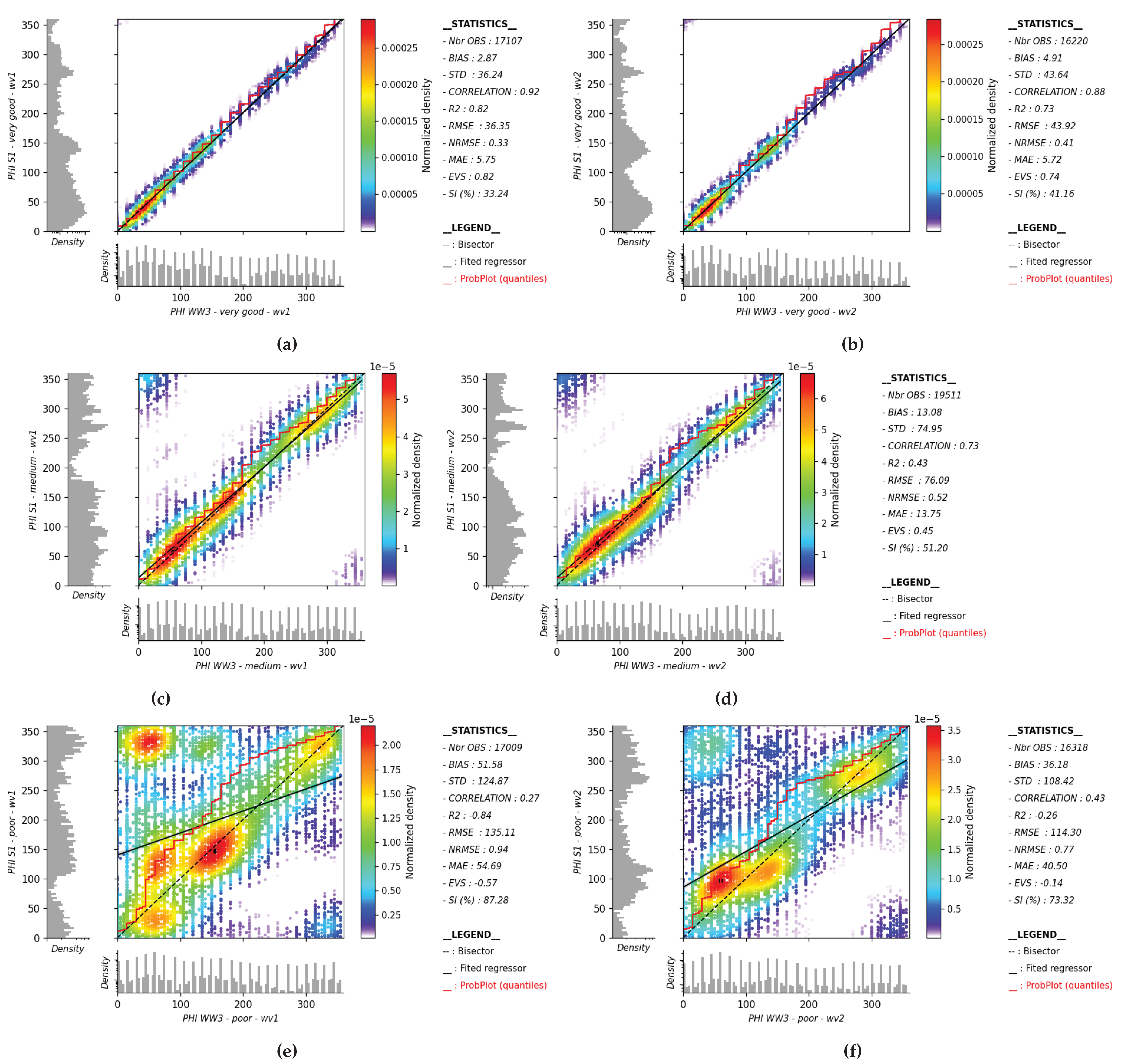
Wave direction in partitions retrieved from the SAR and their colocations with WW3 are presented for the Very Good, Medium, and Poor classes. Panels (a), (c), and (e) correspond respectively to WV1, while panels (b), (d), and (f) correspond respectively to WV2.
Figure A1.
Wave direction in partitions retrieved from the SAR and their colocations with WW3 are presented for the Very Good, Medium, and Poor classes. Panels (a), (c), and (e) correspond respectively to WV1, while panels (b), (d), and (f) correspond respectively to WV2.
Appendix B. Partitions Classification Performed on Peak Wavelength
Figure A2.
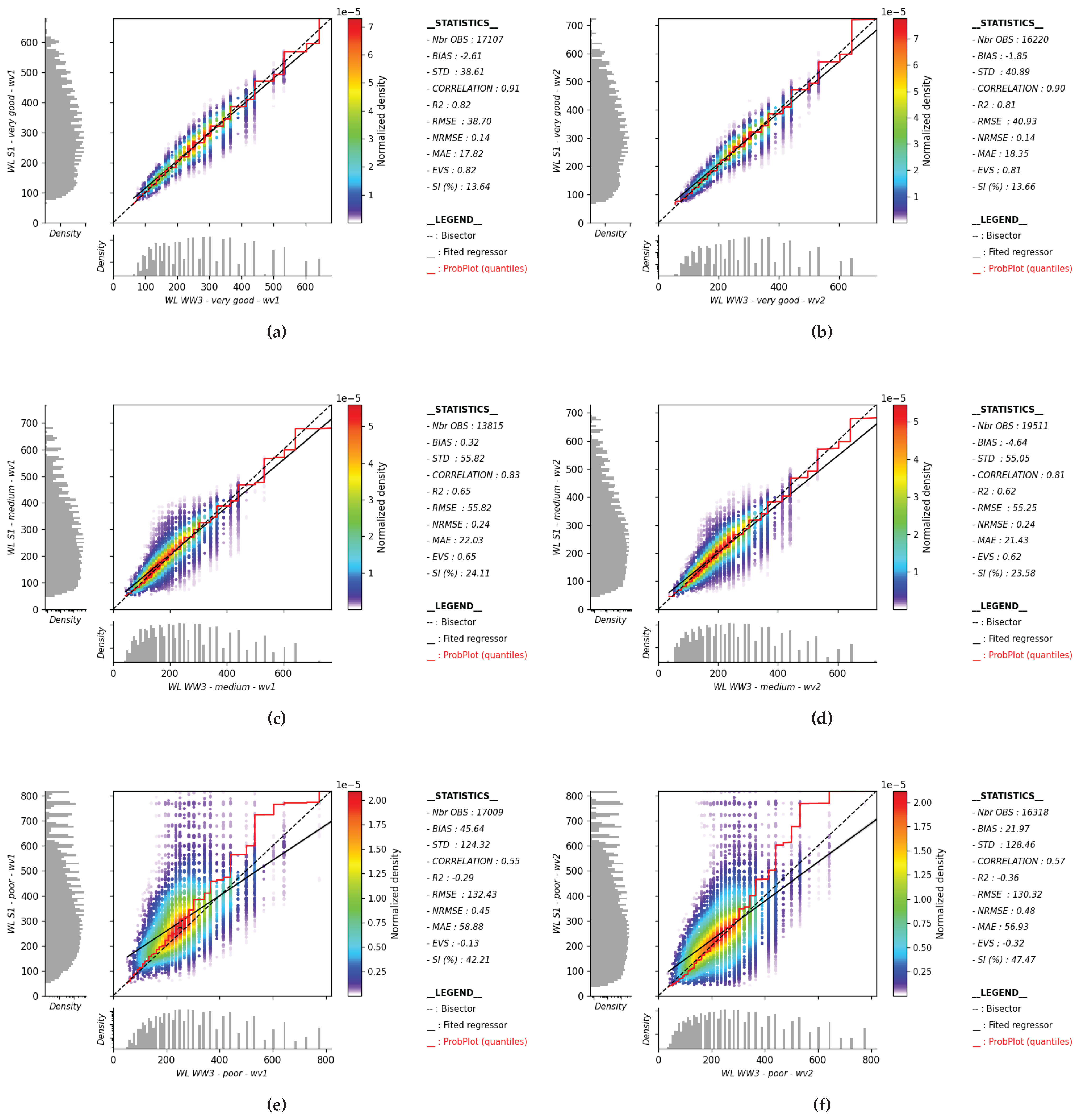
Partition wavelength retrieved from the SAR and their colocations with WW3 are presented for the Very Good, Medium, and Poor classes. Panels (a), (c), and (e) correspond respectively to WV1, while panels (b), (d), and (f) correspond respectively to WV2.
Figure A2.
Partition wavelength retrieved from the SAR and their colocations with WW3 are presented for the Very Good, Medium, and Poor classes. Panels (a), (c), and (e) correspond respectively to WV1, while panels (b), (d), and (f) correspond respectively to WV2.
References
- Ardhuin, F.; Chapron, B.; Collard F. Observation of swell dissipation across oceans. Geophys. Res. Lett., 2009, 36. [CrossRef]
- Ardhuin, F. ; Rogers, E.; Babanin, A.V. ; Filipot, J.-F.; Magne, R.; Roland, A.; van der Westhuysen, A.; Queffeulou, P.; Lefevre, J.-M.; Aouf, L.; Collard, F. Semiempirical dissipation source functions for ocean waves. Part I: Definition, calibration, and validation. J. Phys. Oceanogr. 2010, 40, 1917-1941. [CrossRef]
- Ardhuin, F.; Stopa, J.; Chapron, B.; Collard, F.; Smith, M.; Thomson, J.; et al. Measuring ocean waves in sea ice using SAR imagery: A quasi-deterministic approach evaluated with Sentinel-1 and in situ data. Remote Sens. Environ. 2017, 189(Supplement C), 211-222. [CrossRef]
- Brüning, C.; S. Hasselmann, K.; Hasselmann, K.; Lehner, S.; Gerling, T. W. First evaluation of ERS-1 synthetic aperture radar wave mode data. Global Atmos. Ocean Syst. 1994, 2, 61–98.
- Chapron, B. ; Johnsen, H. ; Garello, R. Wave and wind retrieval from SAR images of the ocean. Ann. Telecommun. 2001, 56, 682–699.
- Charbonnier, P.; Blanc-Feraud, L.; Aubert, G. and Barlaud, M. Deterministic edge-preserving regularization in computed imaging. IEEE Transactions on Image Processing 1997, 6, 2, 298-311. [CrossRef]
- Chen, T.Q.; Guestrin, C.; Assoc Comp, M. XGBoost: A scalable tree boosting system. In Proceedings of the 22nd ACM SIGKDD International Conference on Knowledge Discovery and Data Mining (KDD), San Francisco, CA, USA 13–17 August 2016 pp. 785–794. [CrossRef]
- Collard, F.; Ardhuin, F.; Chapron, B. Monitoring and analysis of ocean swell fields from space: New methods for routine observations. J. Geophys. Res. 2009, 114, C07023. [CrossRef]
- Delpey, M.T.; Ardhuin, F.; Collard, F.; Chapron, B. Space-time structure of long ocean swell fields. J. Geophys. Res. Ocean. 2010, 115, 1–13. [CrossRef]
- Hastie,T. ; Tibshirani, R. and Friedman, J. The Elements of Statistical Learning, ser. Springer Series in Statistics. New York, NY, USA: Springer New York Inc., 2001.
- Hasselmann, K.; Raney, R.K.; Plant, W.J.; Alpers, W.; Shuchman, R.A.; Lyzenga, D.R.; Rufenach, C.L.; Tucker, M.J. Theory of synthetic aperture radar ocean imaging: A MARSEN view. J. Geophys. Res. 1985, 90 (C3), 4659-4686. [CrossRef]
- Hasselmann, K., Hasselmann, S. On the nonlinear mapping of an ocean wave spectrum into a synthetic aperture radar image spectrum and its inversion. J. Geophys. Res. 1991, 96 (C6), 10713-10729. [CrossRef]
- Hasselmann, S.; Brüning, C.; Hasselmann, K.; Heimbach. P. An improved algorithm for retrieval of ocean wave spectra from synthetic aperture radar image spectra. J. Geophys. Res. 1996, 101, 16 615–16 629.
- Husson, R. Development and Validation of a Global Observation-Based Swell Model Using Wave Mode Operating Synthetic Aperture Radar. Ph.D. Thesis, Université de Bretagne Occidentale, Brest, France, 2012.
- Khan, S.S; Echevarria, E.R.; Hemer, M.A. Ocean swell comparisons between Sentinel-1 and WAVEWATCH III around Australia. J. Geophys. Res. 2021, 126(2). [CrossRef]
- Gokcesu, K; Gokcesu, H. Generalized Huber Loss for Robust Learning and its Efficient Minimization for a Robust Statistics. arXiv 2021. [CrossRef]
- Johnsen, H.; Collard, F. Sentinel-1 Ocean Swell Wave Spectra (OSW) Algorithm Definition.Available online :https://sentiwiki.copernicus.eu/web/sentinel-1 (accessed on 5 January 2024).
- Jiang, H., Mouche, A., Wang, H., Babanin, A.V., Chapron, B., Chen, G. Limitation of SAR quasi-linear inversion data on swell climate: An example of global crossing swells. Remote Sens. 2017, 9, 107. [CrossRef]
- Pedregosa, F.; Varoquaux, G.; Gramfort, A.; Michel, V.; Thirion, B.; Grisel, O.; Blondel, M.; Prettenhofer, P.; Weiss, R.; Dubourg, V.; Vanderplas, J.; Passos, A.; Cournapeau, D.; Brucher, M.; Perrot, M.; Duchesnay, E. Scikit-learn: Machine Learning in Python. Journal of Machine Learning Researc 2011, 12, 2825-2830.
- P. J. Huber, Robust statistics. John Wiley& Sons, 2004, vol. 523.
- Quach, B.; Glaser, Y.; Stopa, J.E.; Mouche, A.A.; Sadowski, P. Deep learning for predicting significant wave height from synthetic aperture radar. IEEE Trans. Geosci. Remote Sens. 2021, 59 (3), 1859–1867. [CrossRef]
- Rascle, N; Ardhuin, F. A global wave parameter database for geophysical applications. Part 2: Model validation with improved source term parameterization. Ocean Model. 2013, 70, pp. 174-188. [CrossRef]
- Stopa, J.E.; Ardhuin, F.; Babanin, A.; Zieger, S. Comparison and validation of physical wave parameterizations in spectral wave models. Ocean Model. 2016, 103, 2–17. [CrossRef]
- European Space Agency, “Sentinel-1 User guide”. Available online: https://sentinel.esa.int/web/sentinel/user-guides/sentinel-1-sar/acquisition-modes/wave (accessed on 10 January 2024).
- Stopa, J. E.; Sutherland, P.; Ardhuin, F. Strong and highly variable push of ocean waves on Southern Ocean sea ice. Proceedings of the National Academy of Sciences. 2018, 115 (23), 5861–5865. [CrossRef]
- scikt-learn metrics https://scikit-learn.org/stable/api/sklearn.metrics.html (accessed on 26 July 2024).
- SHAP-tool https://shap.readthedocs.io/en/latest/ (accessed on 14 January 2025).
- Tolman, H.L. User Manual and System Documentation of WAVEWATCH III Version 4.18; Techical Note. Publisher: MMAB Contributio, College Park, MA, USA.
- Wang, X., Husson, R., Jiang, H., Chen, G., Gao, G. Evaluation on the capability of revealing ocean swells from sentinel-1a wave spectra measurements. J. Atmos. Ocean. Technol. 2020, 37 (7), 1289-1304. [CrossRef]
- Wang, H.; Mouche, A.; Husson, R.; Grouazel, A.; Chapron, B.; Yang, J. Assessment of Ocean Swell Height Observations from Sentinel-1A/B Wave Mode against Buoy In Situ and Modeling Hindcasts. Remote Sens. 2022, 14, 862. [CrossRef]
- Wang, X; Wang, X.; Ge, L. Validation and calibration of partitioned integral ocean wave parameters from co-polarized synthetic aperture radar data. Remote Sens. Environ. 2023, 287, 113463. [CrossRef]
- XGBoost Documentation. Available online: https://xgboost.readthedocs.io/en/stable/ (accessed on 16 January 2024).
- About Copernicus https://www.copernicus.eu/en/about-copernicus (accessed on 24 July 2024).
- Copernicus Data Space Ecosystem. https://dataspace.copernicus.eu/ (accessed on 15 january 2025).
- wiki Sentinel-1 https://sentiwiki.copernicus.eu/web/sentinel-1 (accessed on 24 July 2024).
Figure 1.
Polar swell spectrum derived from a S1A WV1 imagette on 23 November 2023 at 18:42, accompanied by an illustration of the partitioning process, where each color (black, red, and blue) represents a distinct partition. The figure includes additional acquisition metadata, such as latitude, longitude, wind speed (U10), wind direction, and other relevant details. The circles represent specific key wavelengths (50,100,200 and 400 m). The inversion limitation clearly highlights the impact of the azimuth cutoff effect (magenta color) resulting in incomplete or distorted observations of these waves.
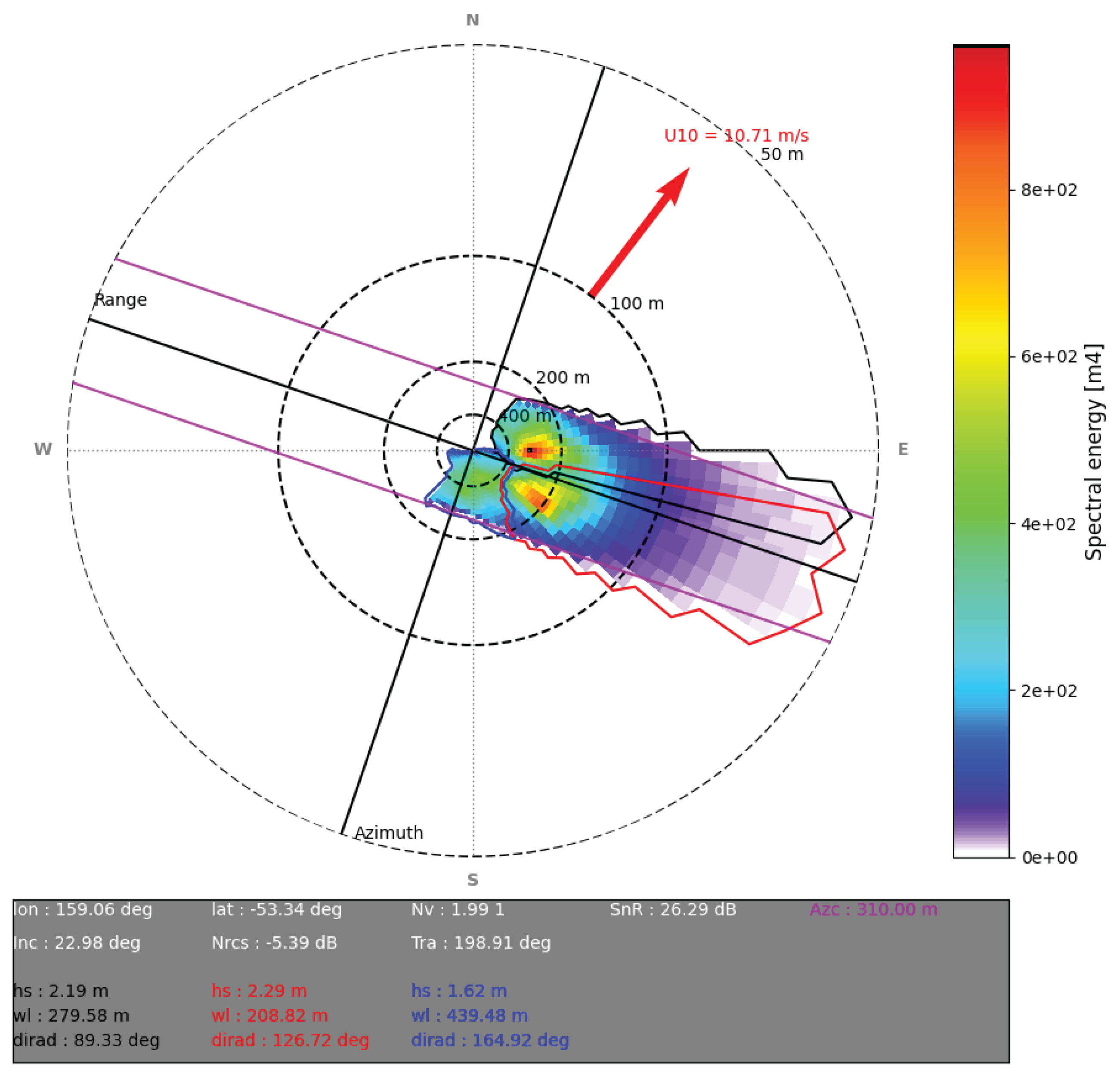
Figure 2.
The effective of partitions, derived from the SAR swell spectrum, along with their colocations with WW3, are presented for the Very Good (first row), Medium (second row), and Poor (third row) classes. Panels (a), (c), and (e) represent WV1, while panels (b), (d), and (f) represent WV2.
Figure 2.
The effective of partitions, derived from the SAR swell spectrum, along with their colocations with WW3, are presented for the Very Good (first row), Medium (second row), and Poor (third row) classes. Panels (a), (c), and (e) represent WV1, while panels (b), (d), and (f) represent WV2.
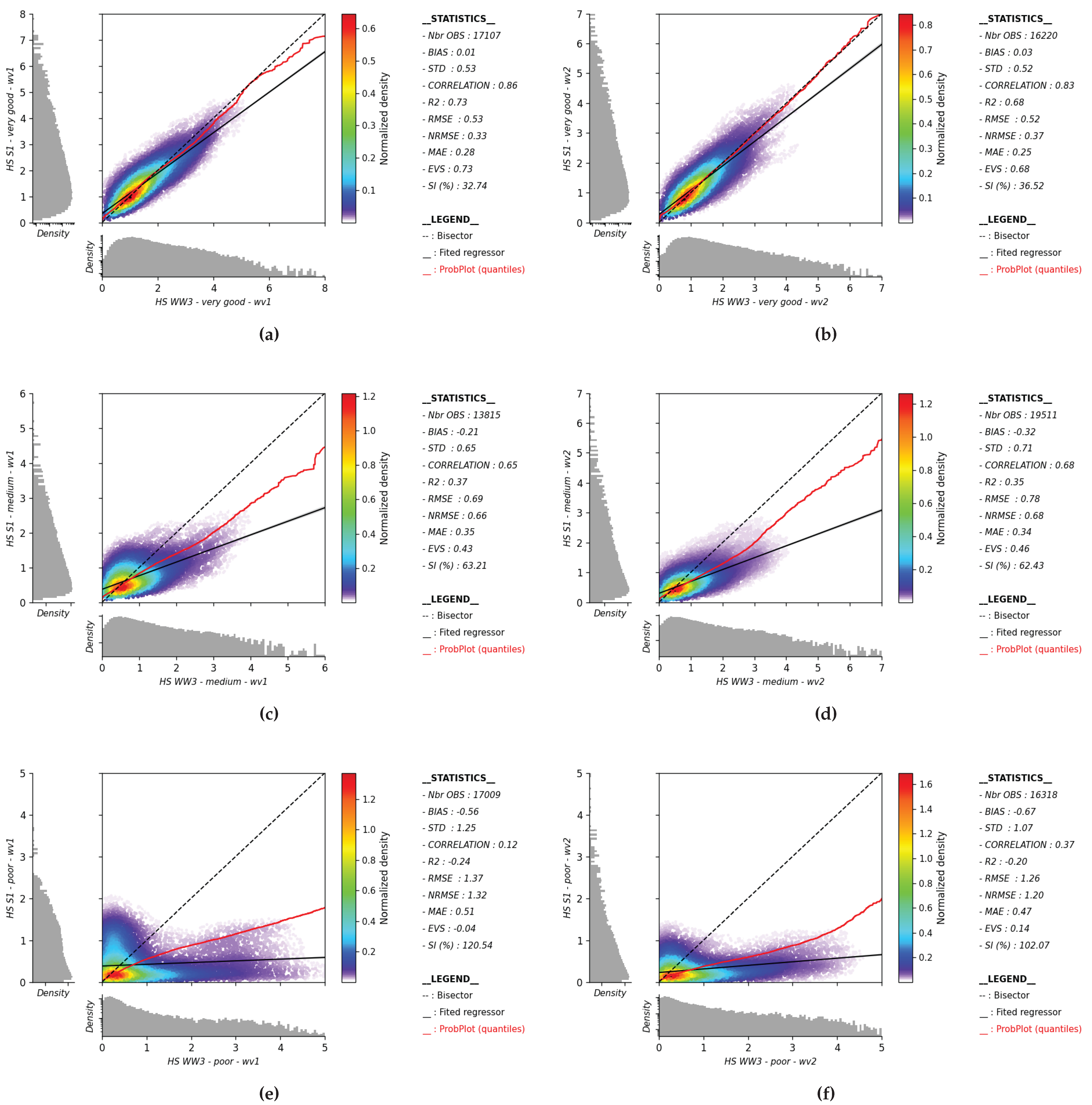
Figure 3.
Quality flag frequency by class for WV1 and WV2, categorized by ascending and descending tracks.
Figure 3.
Quality flag frequency by class for WV1 and WV2, categorized by ascending and descending tracks.
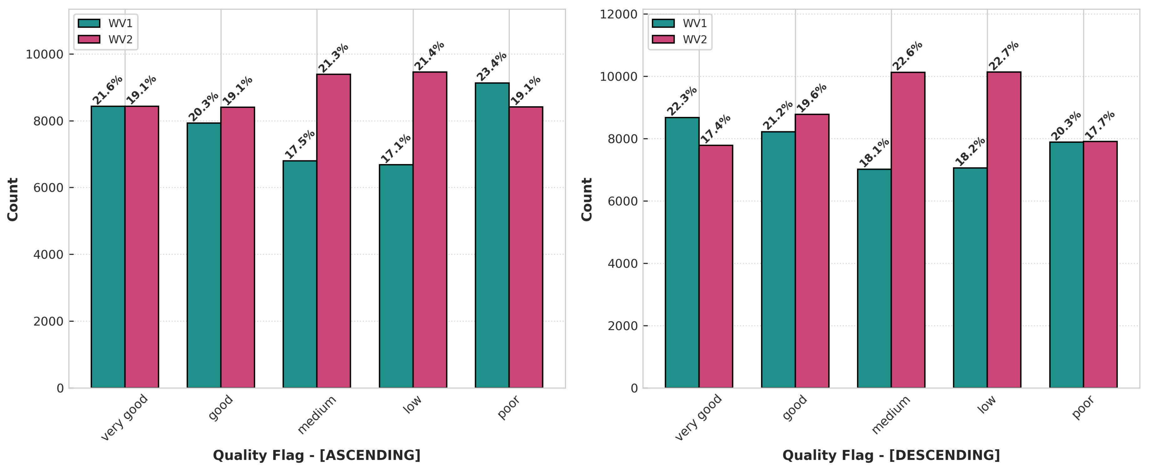
Figure 4.
Partition rank distribution over class for WV1 and WV2, categorized by ascending and descending headings.
Figure 4.
Partition rank distribution over class for WV1 and WV2, categorized by ascending and descending headings.
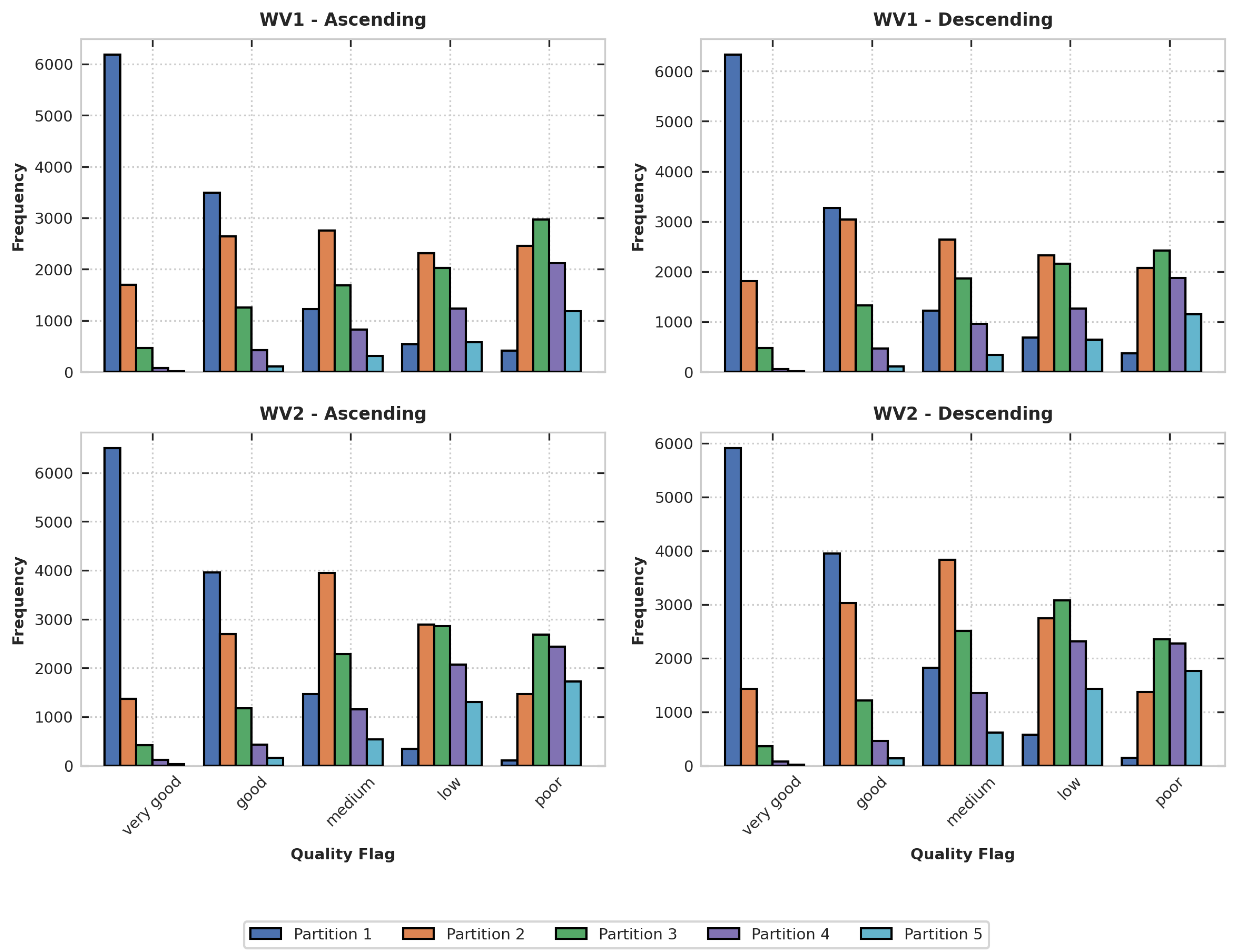
Figure 5.
Spatial Density Distribution of the "Very Good," "Medium," and "Poor" Classes for Both WV1 and WV2.
Figure 5.
Spatial Density Distribution of the "Very Good," "Medium," and "Poor" Classes for Both WV1 and WV2.
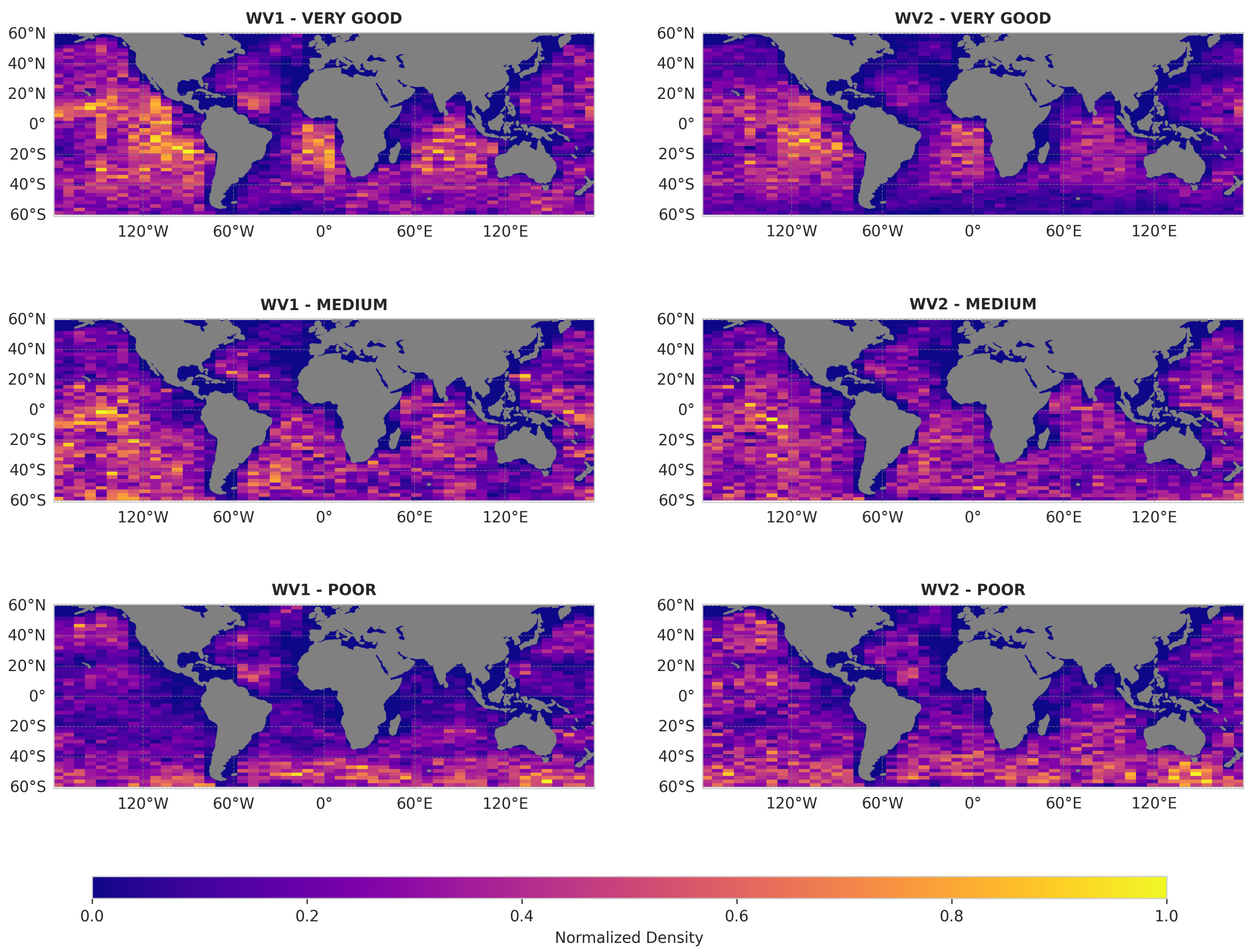
Figure 6.
(a): The swell spectrum derived from a S1A WV1 imagette on 22 November 2023 at 22:04 is presented, with partition quality flags (QF) categorized as follows: Poor QF (red and yellow partitions), Low QF (green partition), Medium QF (black partition), and Good QF (blue partition). This scenario represents downwind conditions, where wave propagation occurs along the satellite’s range axis. The classification indicates that only the Good partition provides reliable data, while the other partitions are flagged as poor due to the inherent limitations of SAR in effectively capturing wave dynamics under these conditions. (b): The NRCS image, which captures a pure ocean swell.
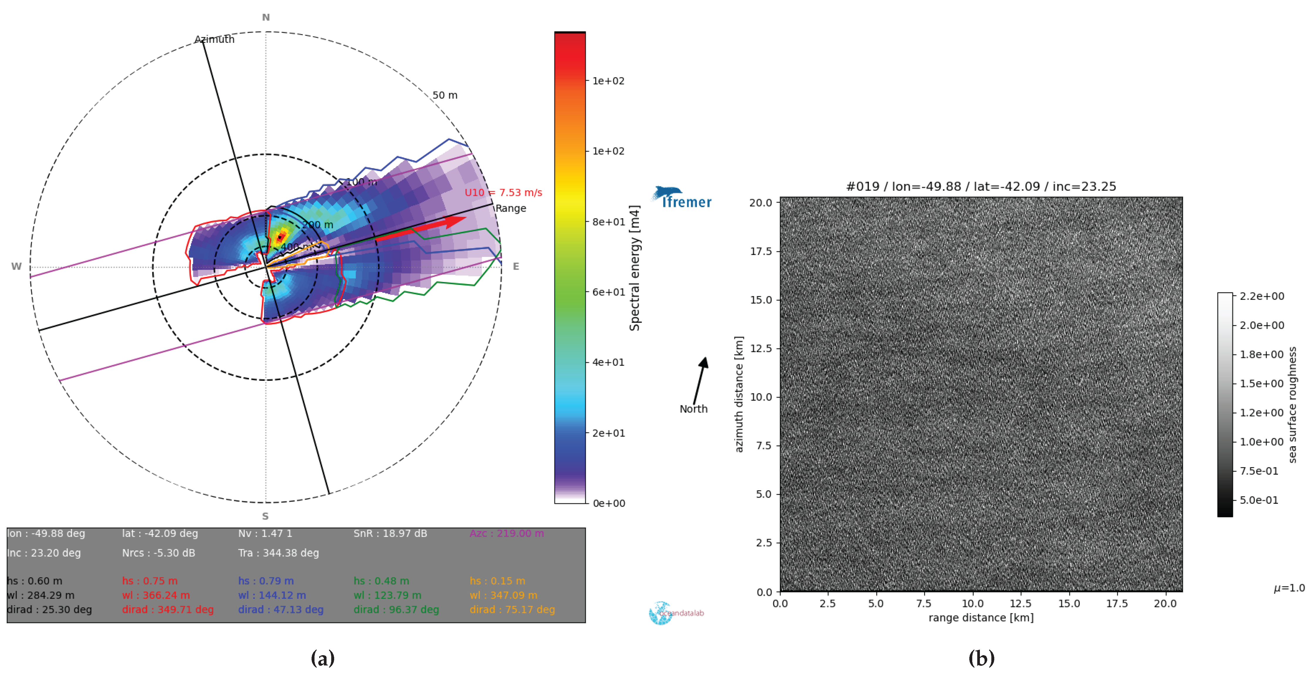
Figure 7.
(a): The swell spectrum from a S1A WV2 imagette taken on 22 November 2023 at 18:02 is shown, with partition quality flags (QF) indicating Low QF (red) and Good QF (black). This acquisition occurs under rain-affected conditions, where the Good partition is considered reliable, and others are flagged due to rain’s impact on the NRCS, which affects wave dynamics. (b): The NRCS image reveals micro convective cells, illustrating how rain phenomena alter radar backscatter and complicate the retrieval of accurate wave information.
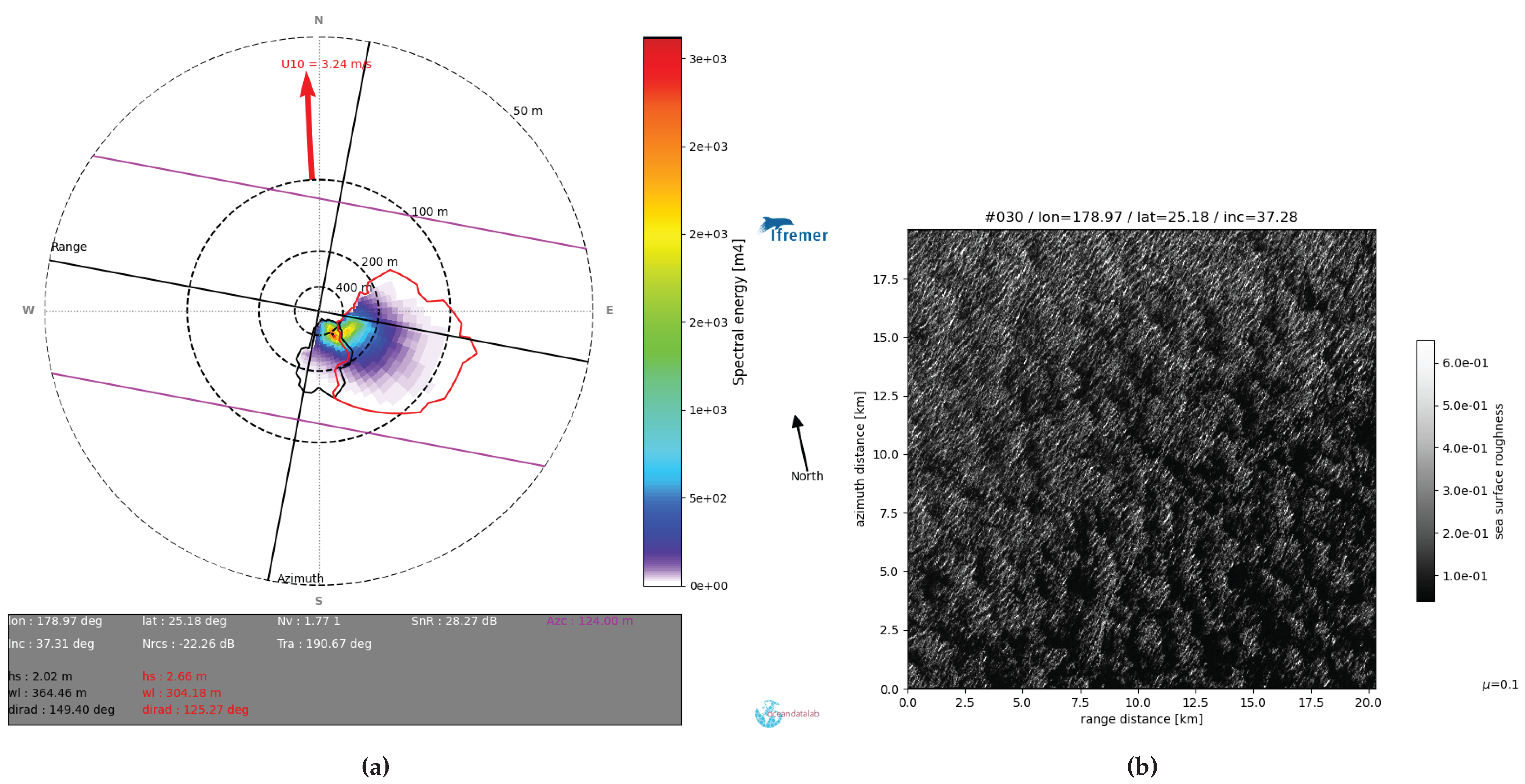
Figure 8.
(a): The swell spectrum derived from a S1A WV2 imagette on 22 November 2023 at 18:07 is shown, with partition quality flags (QF) as follows: Poor QF (green), Medium QF (blue and red), and Good QF (black). This acquisition occurred under atmospheric front conditions, which affect the NRCS and wave dynamics. The classification reveals that only the Good partition provides reliable data, while the others are flagged as poor due to the impact of atmospheric phenomena on radar backscatter. (b): The corresponding NRCS image shows the atmospheric front’s influence, highlighting how such conditions can complicate accurate wave retrieval by altering radar signal returns.
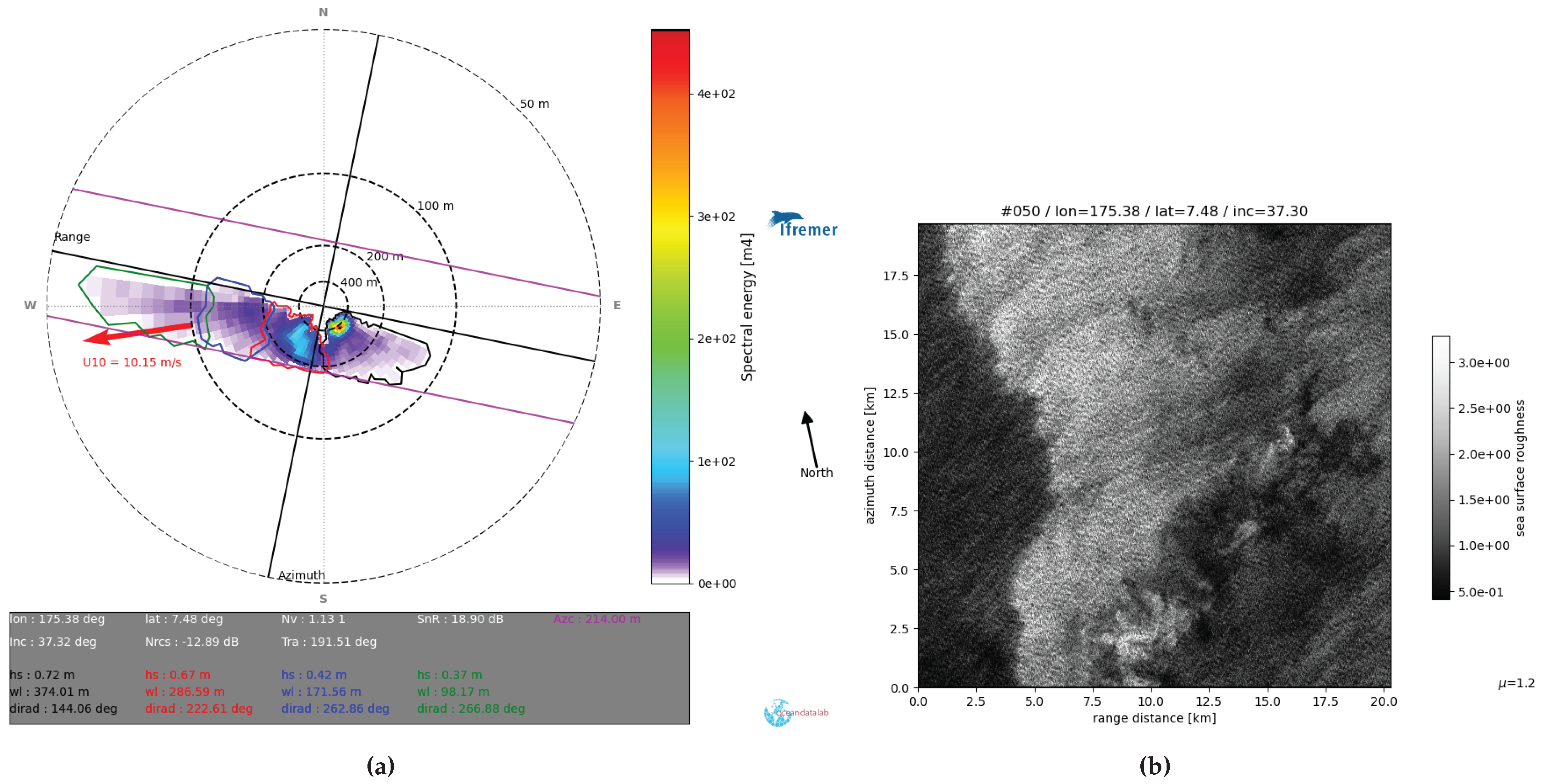
Figure 9.
(a) SHAP-based model explanation for prediction in WV1 configuration: This plot illustrates how various feature values (high values in red, low values in blue) influence the model’s output for prediction in the WV1 configuration, indicating either a positive or negative contribution. Features are ranked by their overall importance, and the dispersion of SHAP values for each feature provides insight into both the strength and direction of its impact on the final prediction. (b) SHAP bar plot showing the mean absolute value of each feature across all instances and grouped by redundancy: This SHAP bar plot displays the average magnitude of each feature’s contribution to the model’s predictions. The length of each bar represents the mean absolute SHAP value for that feature, quantifying its average influence on the model’s output. Redundant features are grouped together based on a clustering cutoff set at 50%.
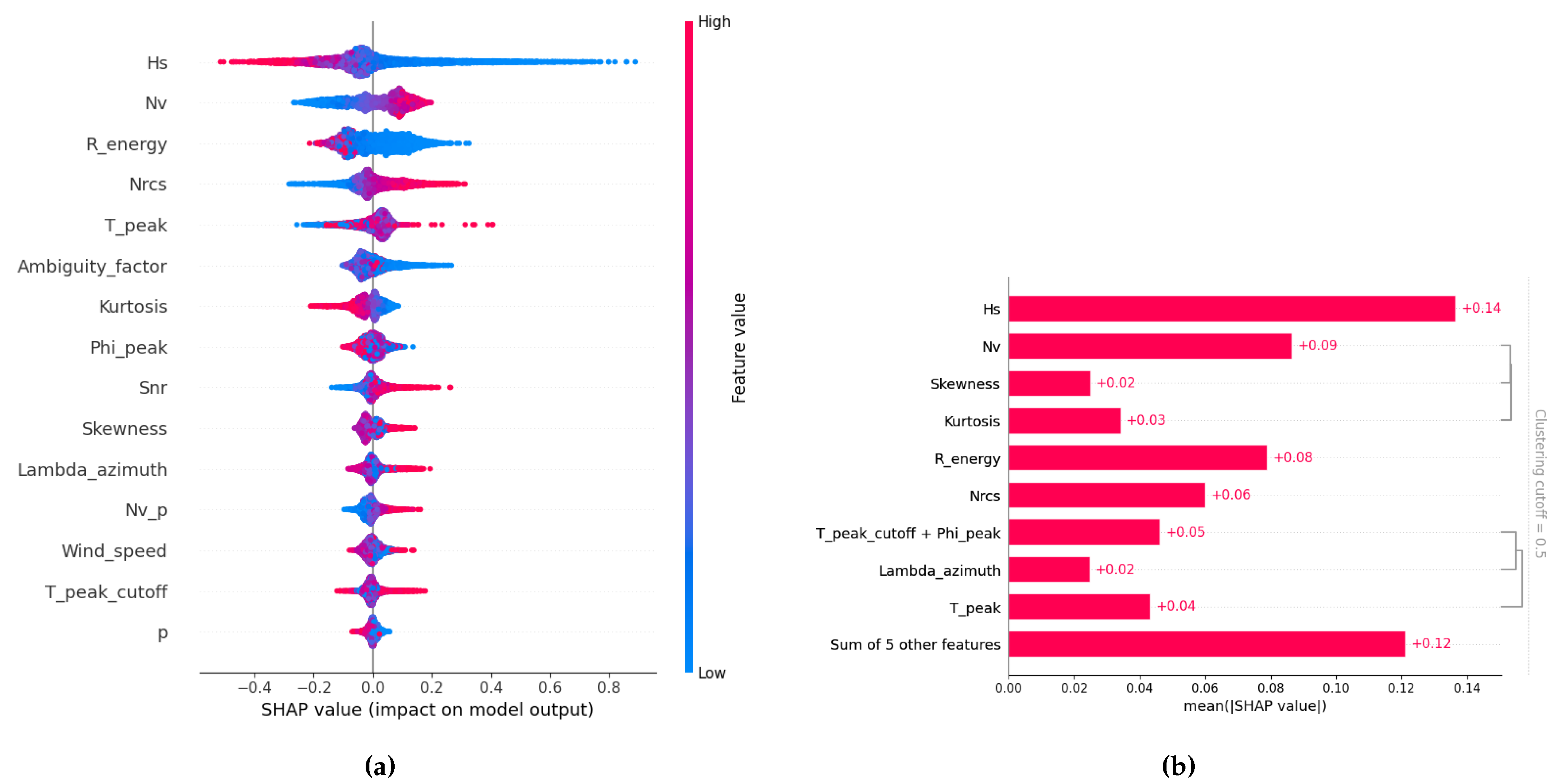
Figure 10.
(a) SHAP-based model explanation for prediction in WV1 configuration: This plot illustrates how various feature values (high values in red, low values in blue) influence the model’s output for prediction in the WV1 configuration, indicating either a positive or negative contribution. Features are ranked by their overall importance, and the dispersion of SHAP values for each feature provides insight into both the strength and direction of its impact on the final prediction. (b) SHAP bar plot showing the mean absolute value of each feature across all instances and grouped by redundancy: This SHAP bar plot displays the average magnitude of each feature’s contribution to the model’s predictions. The length of each bar represents the mean absolute SHAP value for that feature, quantifying its average influence on the model’s output. Redundant features are grouped together based on a clustering cutoff set at 50%.
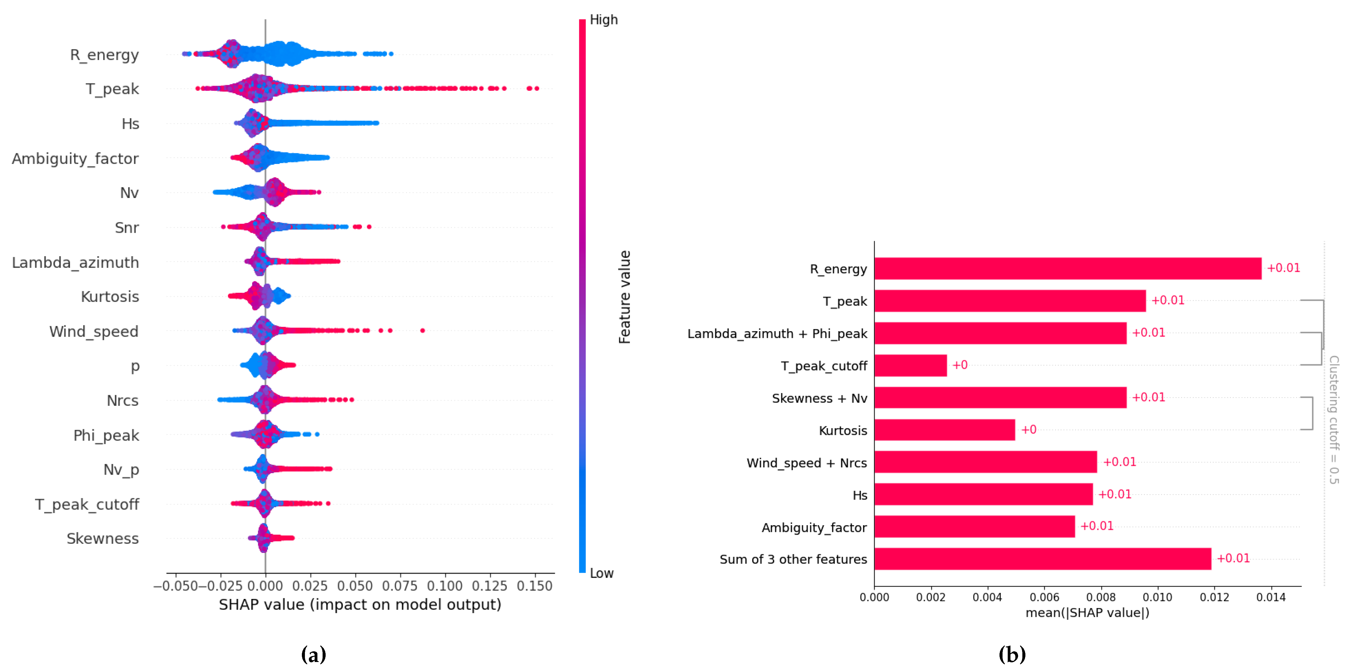
Figure 11.
(a) SHAP-based model explanation for prediction in WV1 configuration: This plot illustrates how various feature values (high values in red, low values in blue) influence the model’s output for prediction in the WV1 configuration, indicating either a positive or negative contribution. Features are ranked by their overall importance, and the dispersion of SHAP values for each feature provides insight into both the strength and direction of its impact on the final prediction. (b) SHAP bar plot showing the mean absolute value of each feature across all instances and grouped by redundancy: This SHAP bar plot displays the average magnitude of each feature’s contribution to the model’s predictions. The length of each bar represents the mean absolute SHAP value for that feature, quantifying its average influence on the model’s output. Redundant features are grouped together based on a clustering cutoff set at 50%.
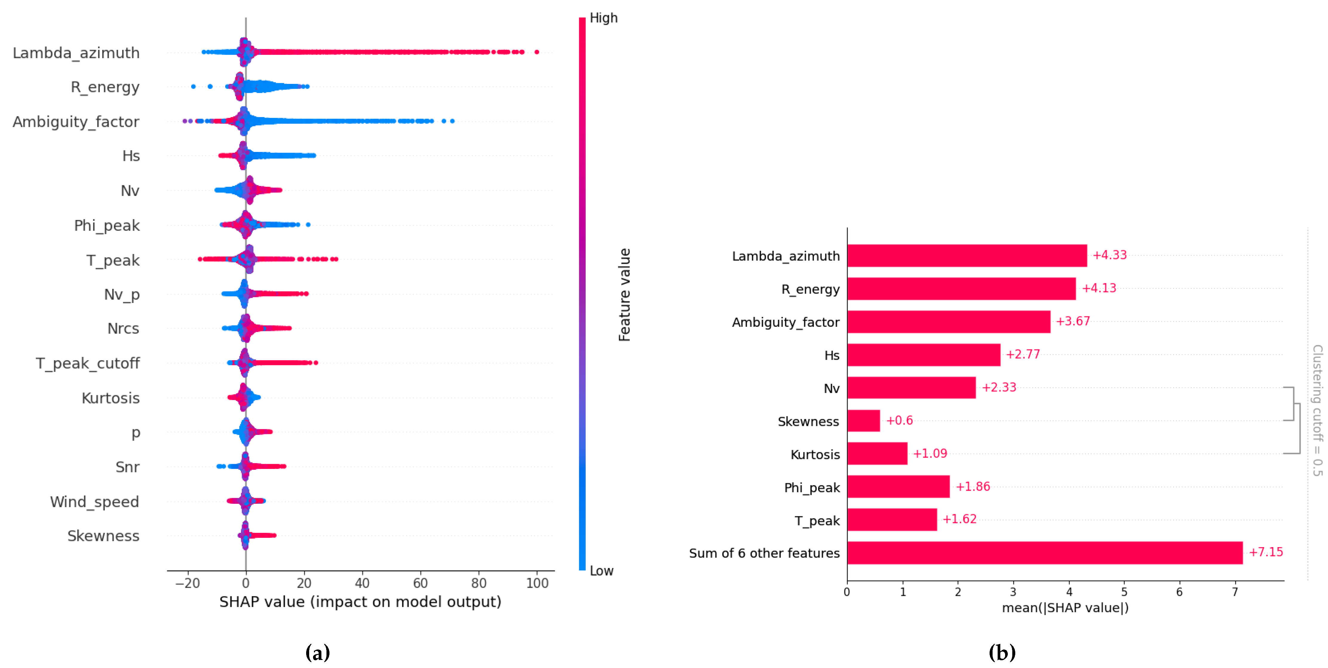

Table 1.
SAR features used to learn partition integral parameter error.
| Feature | description |
|---|---|
| p | The partition index |
| The significant wave height in the partition p | |
| The dominant wave direction in the partition p projected in the SAR geometry | |
| The dominant wavelength in the azimuth direction in the partition p | |
| The normalized variance of significant wave height in the partition p | |
| The energy ratio between the partition energy peak and the maximum boundary energy | |
| The wave peak period in the azimuth cutoff direction in the partition p | |
| The wave peak period in the partition p | |
| The absolute value of the ambiguity factor related to wave propagation direction | |
| The Normalized Radar Cross Section of the SLC WV imagette | |
| The estimated SAR wind speed at 10 m from the SLC WV imagette | |
| The Signal to Noise Ratio (SNR) of the SLC WV imagette | |
| The Skewness of the SLC WV imagette | |
| The kurtosis of the SLC WV imagette | |
| The normalized variance of the SLC WV imagette |
Table 2.
The main XGBoost hyperparameters selected for tuning.
| Hyperparameter | Range | Default | Search range | Definition |
|---|---|---|---|---|
| (0,1] | 1 | [0.7,1] | The fraction of features that will be used to construct each tree | |
| [0,1] | 0.3 | [0.01,0.4] | Step size at each iteration while the objective function is being optimized | |
| [0,∞) | 6 | [4,10] | The maximum depth of each tree | |
| [0,∞) | 1 | [5,10] | Maximum number of nodes to be added | |
| [0,∞) | 1 | [5,15] | Number of parallel trees constructed during each iteration | |
| (0,1] | 1 | [0.7,1] | The proportion of data that will be sampled for each tree | |
| [0,1) | 100 | [100,300] | The highest number of gradient-boosted trees | |
| [0,∞) | 0 | [0,0.5] | Minimum loss reduction necessary to create a new partition on a tree leaf node | |
| [0,∞) | 0 | [0,10] | L1 regularization term on weights. Increasing this value will make model more conservative | |
| [0,∞) | 1 | [0,10] | L2 regularization term on weights. Increasing this value will make model more conservative |
Table 3.
Performance of quality flags by acquisition mode (WV1, WV2) for partition effective Hs.
| Quality flag | |||
|---|---|---|---|
| Very Good | (0.73, 0.68) | (0.53, 0.52) | (32.74, 36.52) |
| Good | (0.54, 0.53) | (0.58, 0.65) | (50.16, 51.06) |
| Medium | (0.37, 0.35) | (0.69, 0.78) | (63.21, 62.43) |
| Low | (0.14, 0.12) | (0.87, 0.94) | (86.77, 78.67) |
| Poor | (-0.24, -0.20) | (1.37, 1.26) | (120.54, 102.07) |
Table 4.
Performance of quality flags by acquisition mode (WV1, WV2) for partition peak wavelength.
| Quality flag | |||
|---|---|---|---|
| Very Good | (0.82, 0.81) | (38.70, 40.93) | (13.64, 13.66) |
| Good | (0.76, 0.74) | (45.86, 45.87) | (18.97, 18.27) |
| Medium | (0.65, 0.62) | (55.82, 55.25) | (24.11, 23.58) |
| Low | (0.48, 0.42) | (71.85, 71.36) | (28.85, 29.98) |
| Poor | (-0.29, -0.36) | (132.43, 130.32) | (42.21, 47.47) |
Table 5.
Performance of quality flags by acquisition mode (WV1, WV2) for partition wave peak direction.
Table 5.
Performance of quality flags by acquisition mode (WV1, WV2) for partition wave peak direction.
| Quality flag | |||
|---|---|---|---|
| Very Good | (0.82, 0.73) | (36.35, 43.92) | (33.24, 41.16) |
| Good | (0.52, 0.52) | (70.03, 67.15) | (49.50, 49.22) |
| Medium | (0.37, 0.43) | (82.07, 76.09) | (53.20, 51.20) |
| Low | (-0.05, 0.21) | (103.99, 90.72) | (68.25, 59.30) |
| Poor | (-0.84, -0.26) | (135.11, 114.30) | (87.28, 73.32) |
Disclaimer/Publisher’s Note: The statements, opinions and data contained in all publications are solely those of the individual author(s) and contributor(s) and not of MDPI and/or the editor(s). MDPI and/or the editor(s) disclaim responsibility for any injury to people or property resulting from any ideas, methods, instructions or products referred to in the content. |
© 2025 by the authors. Licensee MDPI, Basel, Switzerland. This article is an open access article distributed under the terms and conditions of the Creative Commons Attribution (CC BY) license (http://creativecommons.org/licenses/by/4.0/).
Copyright: This open access article is published under a Creative Commons CC BY 4.0 license, which permit the free download, distribution, and reuse, provided that the author and preprint are cited in any reuse.


