Submitted:
21 July 2025
Posted:
22 July 2025
You are already at the latest version
Abstract
There is a significant demand for flexibility in steam turbines, including rapid cold starts and load changes, as well as operation at low partial loads. Both industrial plants and systems for electricity and heat generation are impacted. These new operating modes result in complex, asymmetric temperature fields and additional thermally induced stresses. These lead to casing deformations, that affects blade tip gap and casing flange sealing integrity.The exact progression of heat flux and heat transfer coefficients within the cavities of steam turbines remains unclear. The current methods used in calculation departments rely on simplified, averaged estimates, despite the presence of complex flow phenomena. These include swirling inflows, temperature gradients, impinging jets, unsteady turbulence, and vortex formation.This paper presents a novel sensor and its thermal measurements taken on a full-scale steam turbine test rig. Numerical calculations were performed concurrently. The results were validated by measurements. Additionally, the distribution of heat transfer coefficient along the cavity was analysed. The rule of L'Hôpital was applied at specific locations. A method for handling axial variation of heat transfer coefficient is also proposed. Measurements were taken under real-life conditions at a full-scale test rig at MAN Energy Solutions SE, Oberhausen, with steam parameters of 400 °C and 30 bar. Results for various operating points are presented.
Keywords:
steam turbine
; conjugate heat transfer
; test rig
; thermal measurement
; heat transfer coefficient
; CFD
1. Introduction
There is a growing demand for increased flexibility in modern steam turbines, both in Germany [1] and globally [2]. Notably, there is a demand for quick-start capability, which refers to the turbine’s ability to provide the desired output as rapidly as possible. Furthermore, all applications require multiple design points at partial load, rather than a limited set in the upper fifth of the power range. This requirement extends across thermal, mechanical, and electrical power.
Numerous papers and patents address the issue of rapid cold starts, focusing on modern drive methods that enable faster component warm-up. Gobrecht et al. [3,4] proposes a technique in which the flow path downstream of the intermediate pressure turbine is sealed, thereby increasing the pressure and saturation temperature, which facilitates a quicker heating of the front machine components. The initial parameters for the high-pressure turbine are specified as 620 °C and 300 bar, with reported time saving of one hour. Quinkertz [5] suggests the use of externally generated steam and bypassing the last stage.
Thermal loads can vary due to different process heat requirements. These may involve facilities in the paper industry, chemical industry, district heating systems or other sectors. Mechanical power refers to steam turbines, which, for instance, are employed as drives for large machinery and systems. Electrical power pertains to the flexible generation of electricity. This controllability is crucial for stabilising power grids. This is of particular importance during the energy transition in many European and North American countries, especially when renewable energy sources are prioritised for grid integration.
Operation at partial load leads to significant thermal changes in the steam turbine components, some of which are subject to high stress, particularly due to load changes [6]. Through open and closed circumferential segments mass flow can be saved in comparison to throttle control [7]. However, the machines are supplied with live steam asymmetrically. Control stages mitigate this effect, but do not completely equalise it. Consequently, hot circulating flow regimes develop, which also heat up the contacting components significantly. This can cause hotter spots and colder spots, meaning transient operation sometimes results in high thermal stresses. These must be investigated to design steam turbine components under high thermal loads in terms of mechanical load and lifetime prediction [8].
Modern measurement technology must recognise and meet the state of the art requirements. This concerns temporal resolution and enhanced measurement accuracy. Kaiser [9] provides a comprehensive overview of thermal measurements. This applies in particular to measurements of heat flux sensors based on the principle of substitute walls. The medium of steam is considerably more complex to experiment with than using tempered compressed air. In addition, operation needs much more know-how, is expensive, especially in terms of components and manpower and time-consuming. Moreover, moisture can cause short circuit in electrically exposed conductors. Nevertheless, new types of sensors must be developed in order to demonstrate predicted effects. For this purpose, one starts with straightforward measurable effects at easily accessible locations and successively proceed, with measuring success, to more complex phenomena at machine sections that are difficult to access.
Heat transport in side spaces of steam turbines are not fully understood yet. Although steam turbines have been providing electricity and heat for a long time, the specification of thermal boundary conditions is still imprecise in some machine sections. Numerical engineers require valid measurement data as reference points for the specification of thermal boundary conditions to correctly calculate thermal expansions during operation, which have an impact on deformation and also on the split flange and its tightness. The component life time is also significantly affected by these influences.
Research on side spaces has been conducted intermittently across the globe. Several studies from Eastern Europe during the 1980s and 1990s focused extensively on steam turbines. At that time, for instance, machines of the type K-200-130 (or bigger) were analysed [10,11,12]. Both casings and valves [13], as well as rotors [14], were investigated. Correlations were established for heat transfer as a function of power for both the rotor and side chambers. The findings of this work are subsequently compared with the existing literature [10].
In the 2010s, several test rigs were set up to investigate heat transfer. Tempered compressed air was often used as medium instead of steam. Spura et al. [15,16,17,18,19] built up a test rig called SiSTeR (Side Space Test Rig). The test rig was equipped with two independent measurement methods to characterise the heat transfer. Computational fluid dynamics (CFD) were done in parallel. The results show good agreement. For the formulation of equations of heat transfer along the rotor axis, functions similar to Gaussian distributions (“bell curve”) were established.
Adinarayana [20] build up a 1:2 test rig pressurised with steam for thermal measurement. This work incorporated eight heat flux sensors according to the design of Gardon [21]. The measured values of the heat transfer coefficient exceeded 1000 W/m²K during the start and and remained within the three-digit range during steady-state operation, depending on the measurement position. Moroz et al. [6] performed a thermo-structural analysis during transient operations for a 30 MW steam turbine, which was accompanied by a test campaign on a full-scale test rig. The focus was on modelling and numerical simulation. Therefor, just a few thermocouples on the outer surface of the steam turbine casing were used as initial data. Heat fluxes were not measured. No error bars are given either.
The absence of comprehensive experimental work and corresponding measurement data suggests that there are very few steam-operated test rigs in which heat flows or heat transfers have been measured, or that the manufacturers leave these tests unpublished. The authors are not aware of many studies on full-scale test rigs using heat flux sensors. This scientific gap is intended to be progressively closed with the results of this study.
Experimental and numerical work should ideally be conducted simultaneously. On the one hand, numerical codes must be validated with experimental data. On the other hand, functional codes can predict phenomena that may require new experimental investigations. In this way, each discipline can contribute new insights to the other. In the ideal case, experimental and numerical results align.
In this work, a noval thermal sensor was applied to a side space of a steam turbine to improve the knowledge regarding heat transfer. The general setup of the test rig used for experimental investigation presented in this work is described in detail by Brunn et al. [22,23]. Weigel et al. [24] investigated the heat transfer of this machine with focus on transient measurement during start-up. Especially a method was used to measure the adiabatic wall temperature with proprietary sensors.
2. Sensor
The sensor (Figure 1) consists primarily of a measuring rod, a foil and the housing. Thereby, the cylindrical rod is equipped with several sensing elements. The diameter of the rod is approximately 8 mm. The foil provides the connection between the rod and the fluid. The sensor housing protects the electronics and establishes thermal contact with the steam turbine casing (wall). Accordingly, the sensor can be considered to be thermally well coupled.
The temperature field of a casing of a steam turbine can be highly inhomogeneous. This effect may be caused by steam extraction or injection, geometric asymmetries in the casing or operation at partial load, which results in presence of hot circulating flow patterns. Additionally, heat fluxes are superimposed in all directions.
The measuring rod is surrounded by insulating air, enabling the measurement of only the wall-normal (quasi radial) heat flux. Therefore, heat flows in axial or circumferential direction can be eliminated by design. The only possible heat transfer from the rod to the sensor housing is via heat radiation, which is negligible due to the small temperature differences involved.
Seven thermocouples (indicated in orange) are positioned on the rod. Notably, one of these is used as cold junction. It is installed in the centre of the thermocouples (θ3). By using a resistance thermometer, one temperature and six differential temperatures can be measured. This architecture enables the measurement of very low thermoelectric voltages. High amplification and comprehensive protection of the signals ensure high measurement resolution with low noise.
For this type of proprietary thermocouple, the Seebeck coefficient must be determined individually for this specific material pairing selected. Standard turbine steel was used as rod material in this work. This corresponds approximately to the types of thermocouples E and J. These types are characterised by excellent thermoelectric properties, resulting in high transmission factors. The sensor design and the determination of the transmission factor are described in detail in [24]. Thereby, the transmission factors were determined at different reference temperatures.
Another component is the heating unit, which allows for manipulation of the temperature field. Figure 2 presents the time plot of the differential temperatures relative to the cold junction at the centre. Heat fluxes were applied to each of the rod ends. It can be observed that the heat fluxes across the rod are reversed. Consequently, heat fluxes can be measured validly in both directions. The resolution is comparatively high, exceeding 1000 digit/K for steel and exceeding 600 digit/K for nickel-chrome, with low scattering. The sampling rate was approximately 5 Hz.
Using this heating component and a specialised measurement technique, it is possible to measure the adiabatic wall temperature [24]. This method is consistent with those reported in the literature. Pinilla et al. [25] determined adiabatic wall temperatures on turbine vanes using small, double-layered thin film gauges. Laveau et al. [26] investigated a vane passage gap unsing an infrared camera. The results were presented in relation to CFD calculations. Finally, Lavagnoli et al. [27] described potential errors that can occur during the determination of adiabatic wall temperatures.
3. Development of the Results
The following section presents the conditions for obtaining measurement and numerical results. First, the test rig and the measurement setup are presented. Subsequently, the numerical setup is defined.
3.1. Measurement Setup
Test rig
The test rig consists of a full-scale 12 MW steam turbine as shown in Figure 3. The maximum live steam parameters are 400 °C and 30 bar. This machine type can be used for power generation in the form of process heat or district heating, as a driving engine, or to provide electrical power in conjunction with a generator. It is commonly employed as a compressor drive. Four nozzles were provided to achieve partial load, which were controlled by different valves.
Measurement positions
The measurement positions were located in the side space between the intermediate and low-pressure sections. The sensors were installed as substitute walls. Different rod material was selected for the different measuring positions. The last digit represents the circumferential position. The rods at φ =1 (Figure 3) was made of steel, φ=2 was made of nickel-chrome.
The sensors were manufactured as follows. First, a prototype sensor housing was constructed and installed. Initially, it was too large and protruded in the side space. To align the sensor accurately with the inner wall contour the sensor was marked at its final position. Boroscopic images were used to verify the position following the final installation, as shown in Figure 4.
Measurement technique
The purpose is to measure a heat flux perpendicular to the wall (quasi-radial heat flux). This can be attempted using two different thermocouples at different depths. However, this has several disadvantages.
- It does not provide a pure one-dimensional radial measurement, as the thermocouples must be positioned at different locations. Consequently, there is an overlapping lateral and circumferential effect.
- The cold junction is often located in the measuring device or at least outside the machine. As a result, the thermoelectric voltages to be measured are significantly high, leading to considerable measurement uncertainty. This uncertainty inevitably affects the desired measurement result. Independently, grounding issues may introduce further errors in the signal.
- If one sensor fails the resulting data becomes unusable.
In contrast, the sensor design presented here, incorporating seven thermocouples, offers several advantages. Accordingly the measuring rod was insulated using an air gap around it. This meant that axial and circumferential heat fluxes could be prevented. However, the air gap induces a change in the radial thermal resistance of the sensor compared to the steel sensor housing wall. This thermal change caused by the sensor must be considered.
Figure 5 illustrates a sectional view of the turbine wall, both with and without sensor. The application of the sensor induces a change in the thermal resistance of the wall (y- direction: from inside to outside) compared to an original turbine casing made of steel. The thermal resistance increases mainly due to the air gap. It is possible to calculate the change by applying Equations (1) and (2).
The thermal resistance of the sensor consists of a coupled series and parallel connection of individual resistors. The coordinate system depicted for the sensor (Figure 5) includes two directions: y and r. Considering the y-direction first: The foil is connected in series with all other resistors. Considering additionally the r-direction: the sensor housing, the rod and the series connection of air gap and packed stuffing box are arranged in parallel. This procedure can be used to calculate thermal resistances for the original wall, the sensor with steel rod and the sensor with NiCr rod. Subsequently, the resistances can be normalised relative to those of the original wall. The thermal resistance of the original turbine wall is 1 R.
The thermal resistance for the sensor with a steel rod increases by a factor of 1.479, while for nickel-chrome, it increases by a factor of 2.172. Consequently, the heat flux measurement results must be adjusted according to these factors. This method can be considered in light of the results from [24]. As a result, all heat flux measurement values during start-up were higher by the factors described above. Thus, the heat fluxes across the entire heat transfer wall were nearly identical at all measuring positions, when the first hot steam hits the wall, as expected. Table 1 presents the values. The maximum double standard deviation of the measured start-up heat flux values, ranging from (30.89-31.87) kW/m², is below 4 %. The uncertainty of the measurements with steel rod was 2.70 % and with nickel-chrome, it was 3.87 %. In Conclusion it can be stated, that the relative deviation of the averaged values is below 1.70 %, leading to the assumption that the values can be considered equivalent.
The accuracy of the adjustment factors can be confirmed by this measured event, in addition to the established formulas (Equations (1) and (2)) in the literature. Considering the different thermal resistances for each material, the sensors can be regarded as validated.
Uncertainty analysis
The uncertainty analysis includes the significant factors of deviation. These factors are classified into calibration, measurement, and mechanical deviations, as described below.
-
calibration:
- ○
- deviation of the temperature calibrator (0.13 %)
- ○
- 2σ of the measured values used for calibration (0.31 %)
- ○
- deviation of the calibration fit (0.12 %)
-
measuring
- ○
- 2σ of the measured values used for measurement (depending on measuring point)
-
mechanical
- ○
- manufacturing tolerances for length, area, volume (1-2 %)
3.1. Numerical Setup
The program ANSYS Workbench 2020 R2 was used for this paper. For fluid dynamics ANSYS CFX was selected. The mesh represents a 3°-segment of a circle of the upper casing. It includes both fluid and solid domains (Figure 6: A: fluid, B-E: solid), allowing for the calculation of fluid-structure interaction effects. In the fluid domain, inflation layers were applied to resolve the boundary layer. Twenty-five layers with a growth rate of 1.2 were selected for this purpose.
Four different meshes were examined for the calculation (Table 2). Thereby the number of nodes was increased from 180k to 22.5 million. Finally, the third mesh with 4 million nodes was selected for this study, as a y+ of 0.7 was achieved at the inner surface of the wall of the casing (heat transfer wall, Figure 7). It can be assumed that the near-wall flow effects are resolved with sufficient accuracy. Furthermore, the mesh provides more than 250 elements in the axial direction across the heat transfer wall. The element size was approximately 2 mm, or even smaller.
The total energy model was employed for heat transfer calculations, and the Shear Stress Transport (SST) model was chosen as the turbulence model. This model was chosen because it combines the the k-ε and the k-ω turbulence models. For the flow under consideration, both the wall-bounded effects (k-ω) and the wall-free vortex structures (k-ε) must be accounted for and resolved with sufficient accuracy. Globally, convergence of the root mean square residuals (r) for the velocity components, the energy equation and the turbulence of r = 5e-5 was achieved, or even lower. Table 3 summarises the main boundary conditions.
The general parameter of side space are:
- x=1
- p~2 bar (g)
- T=(130-180)°C
- rotor diameter: 450 mm
- height of the annular gap channel: 90 mm
4. Results
Temperature distribution
The temperature field of the casing is mainly characterised by an axial and a radial gradient across the machine as Figure 8 shows. The axial gradient originates from the live steam valve and the high-pressure turbine, extending to the exhaust steam casing. Thereby the gradient along a guide vane carrier is larger compared to the gradient along a side space, as a larger temperature difference must be reduced within a shorter axial length. Furthermore, heat transfer on the inner side is influenced by the flow regime within the respective side space.
Figure 8 illustrates the temperature distribution at three operating points. It is evident that the temperatures increase with higher machine power. The average temperature in the fluid domain exhibits a similar increase.
The temperature in the heat transfer wall was calculated numerically and measured. Both results are shown in Figure 9. All temperatures were referenced to a maximum temperature, Tmax, which represents the highest temperature observed. This procedure was also applied to the other physical variables. The numerical model shows good agreement with the measurement data. However, the measured data exhibit some scatter, even when accounting for the error bars. This variation can be attributed, on one hand, to the duration of the machine’s operation on the respective measurement day at the given operating point. On the other hand, it is important to consider whether the operating point was reached from a lower or higher starting point. This affects whether the components were already warmed up or still required time to reach the operating temperature. In conclusion, the measured and calculated data are in good agreement.
Velocity field
The velocity field can be divided into different regions with different effects. This is visualised using streamlines, as shown in Figure 10, where red indicates positive radial velocity and blue regions correspond to negative radial velocity. Basically, the fluid domain can be divided into two areas. These are the fraction of the flow that passes through the main flow path. It is characterised by high, almost straight, predominantly axial velocity. Here, the fluid elements only remain in the computational domain for a very short time. The other fraction represents the flow within the side space, or secondary flow, which exhibits complex flow dynamics.
The flow structure in the side space is driven by flow fraction, which is colliding with the end face of the guide vane carrier 3 (Figure 6, component D). Consequently, the flow is deflected radially outward. A radial impingement jet flow is developed, impacting an inclined wall. This leads to the formation of two dominant, poloidal main vortices, located to the left and right of the stagnation point (Figure 10, vortex a and b). The front vortex (a) rotates anti-clockwise, while the rear vortex (b) rotates in the opposite direction. The centre of the rotation of the latter is closer to the exhaust casing. Additionally, smaller, counter-rotating vortices (with reversed vorticity) form in the corner areas (Figure 10, vortices c). A detachment (Figure 10, vortex d) occurs in the radially lower area of the vane carrier 2 (Figure 6, component B), just before the fluid elements leave the side space to the main flow. A counter-rotating vortex is located in this area.
The entire flow regime is superimposed with a swirl rotating around the rotor axis (i.e., in circumferential direction), known as toroidal vortex. Due to different operating points and differently developed swirl, either the poloidal or the toroidal vortex components presumably dominate, overlap and influence each other. However, the influence of the swirl will not be discussed in detail in this paper.
The lateral velocity near the wall, and consequently the wall shear stress at the heat transfer wall, reaches a local maximum near the stagnation point. Due to the continuous enthalpy flow of the impingement jet, the fluid and the wall reach approximately the same temperature at this point. The wall cannot absorb or dissipate heat quickly and therefore remains at the flow temperature. The temperature increases upstream (towards the intermediate pressure section) and decreases downstream.
In relation to the flow velocity, the casing is hotter than the fluid from the stagnation point towards the intermediate pressure section. As a result, the casing heats the medium in this area, and heat flows from the casing wall to the fluid. The reverse occurs downstream of the stagnation point, where the casing is cooler than the steam. Consequently, the steam heats the wall in these areas. This leads to a change in the algebraic sign of the heat flux, which is also accompanied by a change in the sign of the temperature difference, .
Heat flux
Figure 11 illustrates the distribution of heat flux on the heat transfer wall in relation to the dimensionless axial coordinate z*. Positive heat fluxes were measured and calculated for z* < 0.42 (12 MW). A positive value indicates that the heat flux is directed from the wall to the fluid, meaning that heat is being transferred into the control volume of the fluid domain. The authors are not aware of any work that has measured heat flux from the wall to the fluid within a steam turbine casing. For 0.42 < z* (12 MW), the heat flux becomes negative, indicating that heat is transferred from the fluid to the colder wall. At z* = 0.15, a discontinuity in the heat flux curve can be observed. This discontinuity is attributed to a change in the geometry of the casing, where the transition from a predominantly cylindrical body to a cone begins. This transition is realised through a rounding with a large radius.
The negative wall heat fluxes at z* = 0.61 are slightly overestimated by the numerical model used. This discrepancy may arise from the fact that the heat dissipated by the exhaust steam casing is likely underestimated in the model, or from the inability of the flow regime—particularly the swirl—to accurately reproduce heat transfer at this point at the solid-fluid interface.
Nevertheless, there is good agreement between the experimental data and the numerical calculations. Based on the simulations, a distribution of the heat flux across the entire heat transfer wall can be predicted, which is corroborated by the good agreement between the measured and calculated casing temperatures.
Energy balance
In order to develop an approach for modelling the development of the heat flux across the boundaries of the fluid domain, an energy balance was considered. The boundary was located along the fluid-solid interface and was closed by a horizontal area at the inlet of the side space. It was found that there are three sections along the boundary that contribute heat to this domain and three sections that remove heat from it. In addition, dissipative heat energy occurs inside the fluid due to internal friction. However, this effect can be neglected due to its negligible influence. Considering the magnitude of the heat quantities, the dissipative heat component is very small.
Figure 12 shows the six different regions and illustrates the heat affected zones. The fraction that contributes heat is considered first. The majority (45 %) is introduced through the flow entering the side space. 28 % is added by the front part of the heat transfer wall (Figure 6, component C). The remaining portion, approximately one-quarter (27 %), is contributed via guide vane carrier 2 (Figure 6, component B).
The heat-absorbing regions are as follows: 69 % of the heat exits the investigated area through vane carrier 3 (Figure 6, component D). A further 29 % is transmitted to the rear part of the casing (Figure 6, component C). Only 2 % exits the control volume in the form of escaping steam.
Heat transfer coefficient
By using Equation (3), the local heat transfer coefficient can be calculated. Here, the local heat flux and the local wall temperature, and the volumetrically averaged fluid temperature of domain A (Figure 6) are used.
The result is shown in Figure 13. The colour code is as in the previous diagrams: 8 MW - green, 10 MW - orange, 12 MW - blue. The experimental results are represented by triangles, the numerical calculation by squares, the approximated function based on the numerical calculation as a line, and the results from l’Hôspital as diamonds. The approximated function is similar to a skewed Gaussian distribution. A Weibull distribution was chosen for the approximation. All required fits were approximated using least squares with the programme OriginPro 2023.
The numerical values between 0.275 and 0.525 are omitted. This is due to the existence of specific points z0* along the wall, where temperature ∆T → 0 and heat flux → 0 tend towards zero. According to Equation (3), a singularity arises at this point. Therefore, the numerical results develop to ±∞, depending on the sign. This effect makes the results unreliable in this area. This situation corresponds to one of l’Hôspital’s rules, specifically the case “0/0”. Consequently, the limit value can be analysed. For this purpose, the functions of and were approximated, inserted into Equation (4) and the limit value considered. Polynomial functions were used for this purpose. Regarding the heat flux, sine functions can also be applied. If this procedure does not yield a reliable result, the derivatives of the functions can also be used. However, in such cases, a reliable outcome is not always guaranteed, but it may still lead to the desired result as in Figure 13.
An approximation was performed for the progression of the numerical values. For this purpose, the Weibull function was used. The resulting fit demonstrates a sufficiently good agreement. This applies to both the numerical calculations and the results from the l’Hôpital limit evaluation.
At the end the following results are obtained.
5. Conclusions and Outlook
A new sensor for measuring heat transfer onto a steam turbine casing was designed, calibrated, validated, and deployed for measurements in a 12 MW full-scale steam turbine. The primary focus was on thermal measurement in a side space, which was complemented by numerical investigations. A numerical study of the mesh quality was conducted, and the boundary conditions for the respective regions were defined based on measurement data. One of the key outcomes is the temperature distribution on the outer casing of the steam turbine. Data from temperature measurement and numerical simulations yielded identical values. The velocity field was presented and discussed in relation to different flow regimes. Visualisation through streamlines illustrated two dominant vortices. Their effects on the boundary layer near the wall significantly influence heat transfer. Furthermore, both the measured and numerically calculated heat fluxes perpendicular to the wall were presented. A directional change in the heat flux along the axial component was observed. It may be the first time a wall heat flux has been measured within a steam turbine casing, transferring heat from the wall to the fluid. The results for the heat transfer coefficient were also presented for both experimental and numerical data. Additionally, a l’Hôpital analysis was conducted, and a correlation for the distribution of the heat transfer coefficient was developed using a function that describes a skewed Gaussian distribution. Overall, the Weibull distribution provided an excellent approximation for this purpose. The heat transfer coefficient was compared with values from the literature. Finally, the results corroborate findings from other scientific studies. This enhanced understanding will contribute to more accurate numerical boundary conditions and improve the quality of the results. Given the scarcity of studies and measurement data on heat transport in side spaces of steam turbines, the results are of significant scientific importance.
Building on the presented work, the analysis of heat transfer in steam turbines, particularly in side spaces, will be systematically advanced. Sensitive factors with a significant impact must be identified and further analysed.
Acknowledgements
The present study was conducted within the project ECOFLEX 434 (grant number: 03ET7092L; 03ET7090M; 03ET7092M) and TurboGrün AP 4.2 (grant numbers: 03EE5069F) of AG Turbo. It is funded by the Federal Ministry for Economic Affairs and Climate Action of the Federal Republic of Germany and MAN Energy Solutions SE. The responsibility for the content lies solely with its authors.
Abbreviations
The following abbreviations are used in this manuscript:
| CFD | computational fluid dynamics | t | [s] | time | |
| T | [°C] | temperature | |||
| g | gauge | TC | thermocouple | ||
| h | [W/m²K] | heat transfer coefficient | x | [-] | steam quality, coordinate |
| HP | high pressure | ||||
| HTW | heat transfer wall | y | [mm] | coordinate | |
| IAPWS | International Association for the Properties of Water and Steam | y+ | [-] | dimensionsless wall distance | |
| z | [mm] | axial coordinate | |||
| IP | intermediate pressure | z∗ | [-] | dimensionsless axial coordinate | |
| k | [m²/s²] | turbulence kinetic energy | ε | [m²/s³] | turbulent dissipation |
| LP | lower pressure | κ | Weibull shape parameter | ||
| p | [bar] | pressure | λ | [W/mK]; [-] |
heat conductivity; Weibull scale parameter |
| P | [W] | power | |||
| [W/m²] | heat flux | θ | [K] | temperature difference | |
| [-], [mm] | residual, coordinate | σ | standard deviation | ||
| [K/W] | thermal resistant | φ | circumferrential coordinate | ||
| SST | shear stress transport | ω | [1/s] | specific turbulence dissipation | |
| Index | |||||
| cas | casing | reference; cold junction | |||
| exp | experimental | s | series | ||
| f | fluid | st | steel | ||
| max | maximum | stat | static | ||
| min | minimum | tot | total | ||
| Ni | Nickel-chrome | wall | |||
| num | numerical | Weibull | |||
| o | limit | λ | conductivity | ||
| p | parallel | ||||
References
- Klaus, T. et al., “Energieziel 2050 – 100% Strom aus erneuerbaren Quellen”, Umweltbundesamt, Juli 2010.
- International Energy Agency, “World energy outlook 2024”, International Energy Agency. https://www.iea.org/reports/world-energy-outlook-2024, 2024.
- E. Gobrecht, K. Peters, “Verfahren zum Aufwärmen einer Dampfturbine”. EP 1775 429 A1, 12.10.2005.
- E. Gobrecht, K. Peters, “Method for heating a steam turbine”. WO 2007/042523 A2, 19.04.2007.
- R. Quinkertz, “Verfahren zum Aufwärmen einer Dampfturbine”. EP 1 934 434 B1, 02.11.2016.
- L. Moroz, G. Doerksen, F. Romero, R. Kochurov, B. Frolov, “Integrated approach for steam turbine thermo-structural analysis and lifetime prediction at transient operations”, Proceedings of ASME Turbo Expo Turbomachinery Technical Conference and Exposition, Charlotte, USA, June 26-30, 2017.
- M. Schleer, J. Steil, “Increasing the performance of steam turbines at part load by optimizing the control system during operation, Proceedings of Global Power and Propulsion Society, Hong Kong, China, October 17-19, 2023. ISSN-Nr: 2504-4400.
- S. Koliadiuk, M. H. Sulzhenko, “Thermal and stress state of the steam turbine control valve casing, with the turbine operation in the stationary modes”, Journal of Mechanical Engineering, vol. 22, no. 2, 2019. ISSN 0131–2928.
- E. Kaiser, “Zur Wärmestrommessung an Oberflächen: unter besonderer Berücksichtigung von Hilfswand Wärmestromaufnehmern”, habilitation thesis, Dresden, 1981.
- A. S. Leizerovich, “Steam Turbines for Modern Fossil Fuel Power Plants”. Taylor & Francis, Boca Raton, ISBN 1-4200-6102-X, 2008.
- E. R. Plotkin, A. S. Leizerovich and I.V. Muratova, “Investigation of Heat Transfer Conditions in the K-200-130 Turbine,” Thermal Engineering, Vol. 18(5), pp. 41-47, 1971.
- E. R. Plotkin, A. S. Leyzerovich, “Start-ups of Power Unit Steam Turbines”, Moscow: Energiya, 1980.
- O. Chernousenko, D. Rindyuk, V. Peshko, “Research on residual service life of automatic locking valve of turbine K-200-130”, Eastern-European Journal of Enterprise Technologies, ISSN 1729-3774, 2017. [CrossRef]
- S. R. Lishchuk, V. A. Peshko, “Calculation study of thermal stresses in the medium-pressure rotor of the K-200-130 turbine during start-up from a cold state”, Journal of Mechanical Engineering – Problemy Mashynobuduvannia, vol. 27, no. 2, ISSN 2709-2984, 2024. [CrossRef]
- D. Spura, J. Lueckert, S. Schoene, U. Gampe, “Concept Development For The Experimental Investigation Of Forced Convection Heat Transfer In Circumferential Cavities With Variable Geometry”. International Journal of Thermal Sciences Vol. 96: pp. 277–289, 2015. [CrossRef]
- D. Spura, U. Gampe, G. Eschmann, W. Uffrecht, “Experimental Investigation of Heat Transfer in Cavities of Steam Turbine Casings under Generic Test Rig Conditions”. Proceedings of ASME Turbo Expo Turbomachinery Technical Conference and Exposition, Oslo, Norway, June 11-15, 2018. [CrossRef]
- D. Spura, U. Gampe, G. Eschmann, W. Uffrecht, “Experimental Investigation of heat transfer in cavities of steam turbine casings under generic test rig conditions”. Journal of engineering for Gas Turbines and Power, 2018. [CrossRef]
- D. Spura, G. Eschmann, W. Uffrecht, U. Gampe, S. Odenbach, “COOREFLEX 4.3.6: Thermisches und mechanisches Verhalten von Turbinengehäusen: Statusbericht. Tagungsband zum 15. Statusseminar der AG Turbo”. Bergisch-Gladbach, 12.–13.12.2016, 2016. [CrossRef]
- D. Spura, “Untersuchung des lokalen Wärmeübergangs in Seitenräumen von Turbinengehäusen am Beispiel von Industriedampfturbinen”, Dissertation, 2021.
- Adinarayana N, Sastri V M K. “Estimation of convective heat transfer coefficient in industrial steam turbine”. Journal of Pressure Vessel Technology, 1996, 118(2): 247–250.
- Gardon, R., “A Transdcer for Measurement of Heat Flow Rate”, ASME Journal of Heat Transfer, Vol. 82, pp. 396-398, 1960.
- O. Brunn, K. Deckers, T. Polklas, K. Behnke, M.-A. Schwarz, “Experimental and numeric investigations on a steam turbine test rig in part load operation”. Proceedings of 12th European Conference on Turbomachinery Fluid dynamics & Thermodynamics, Stockholm, Sweden, 2017.
- O. Brunn, U. Harbecke, T. Mokulys, V. Salit, M. A. Schwarz, F. Dornbusch, “Improved LP-Stage design for industrial steam turbines”, Proceedings of ASME Turbo Expo Turbomachinery Technical Conference and Exposition, Virtual, September 21-25, 2020.
- B. Weigel, T. Polklas, S. Odenbach, W. Uffrecht, “Thermal Characterization of a steam turbine casing including measuring of adiabatic wall temperatures using proprietary sensors”, Proceedings of ASME Turbo Expo Turbomachinery Technical Conference and Exposition, Virtual, June 7-11, 2021.
- V. Pinilla, J. P. Solano, G. Paniagua, R. J. Anthony, “Adiabatic Wall Temperature Evaluation in a High Speed Turbine”. Journal of Heat Transfer. Vol. 134, Issue 9, 091601, pp 1-9. September, 2012. [CrossRef]
- Laveau, R. S. Abhari, M. E. Crawford, E. Lutum, “High resolution heat transfer measurements on the stator endwall of an axial turbine”. Journal of Turbomachinery 137, 2015. [CrossRef]
- S. Lavagnoli, C. De Maesschalck, G. Paniagua, “Uncertainty Analysis of Adiabatic Wall Temperature Measurements in Turbine Experiments”. The XXII Symposium on Measuring Techniques in Turbomachinery, Transonic und Supersonic Flow in Cascades and Turbomachines, Lyon, France, September 4-5, 2014. [CrossRef]
Figure 1.
Principle of the sensor including the thermocouple positions and other sensor elements on the rod [24].
Figure 1.
Principle of the sensor including the thermocouple positions and other sensor elements on the rod [24].
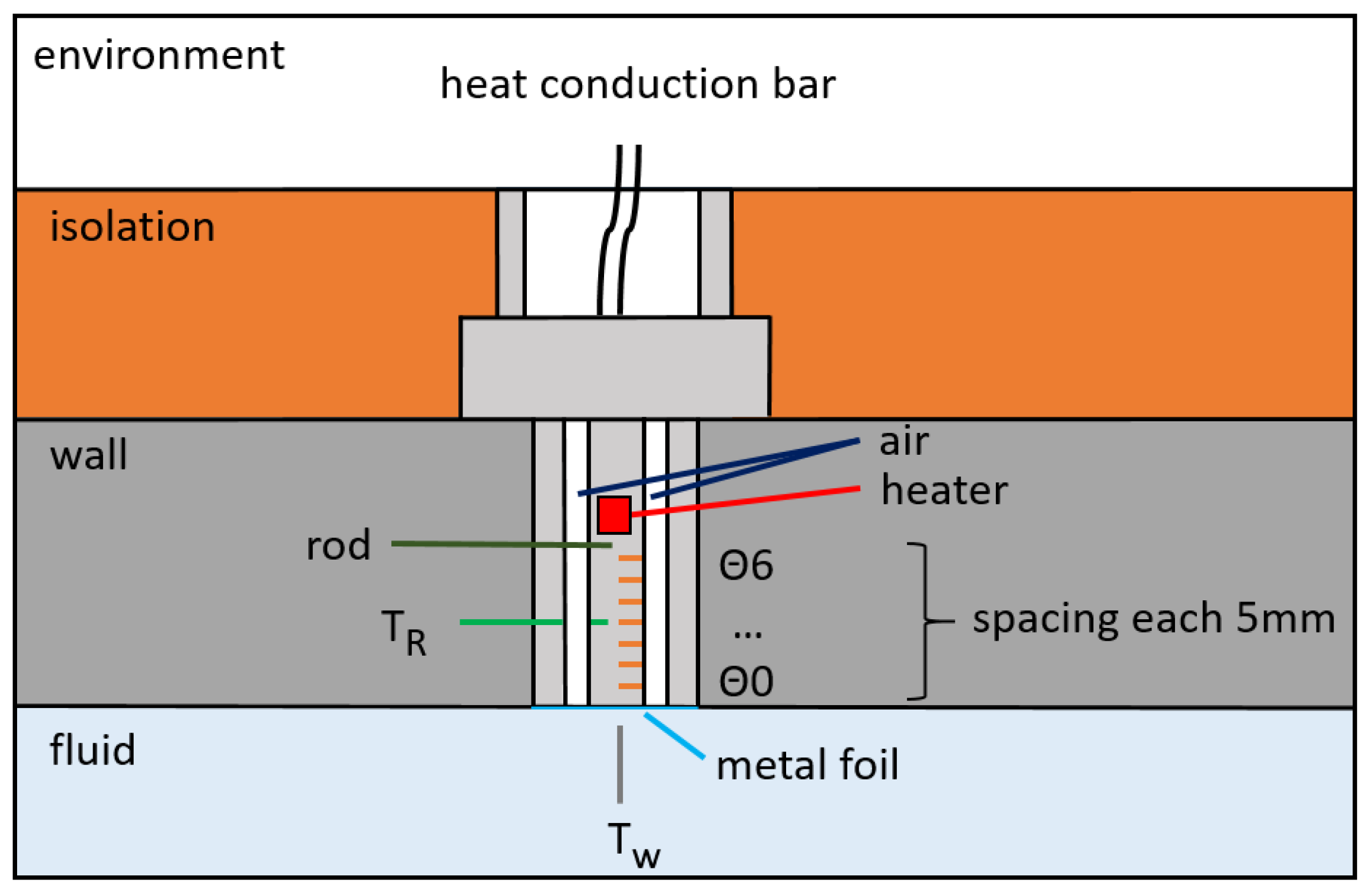
Figure 2.
Functional test: Graph of thermocouple signals while different thermal states. t < 600 s: internal heating via heating unit. t > 600 s: external heating with hot fluid from thermostat at the foil.
Figure 2.
Functional test: Graph of thermocouple signals while different thermal states. t < 600 s: internal heating via heating unit. t > 600 s: external heating with hot fluid from thermostat at the foil.
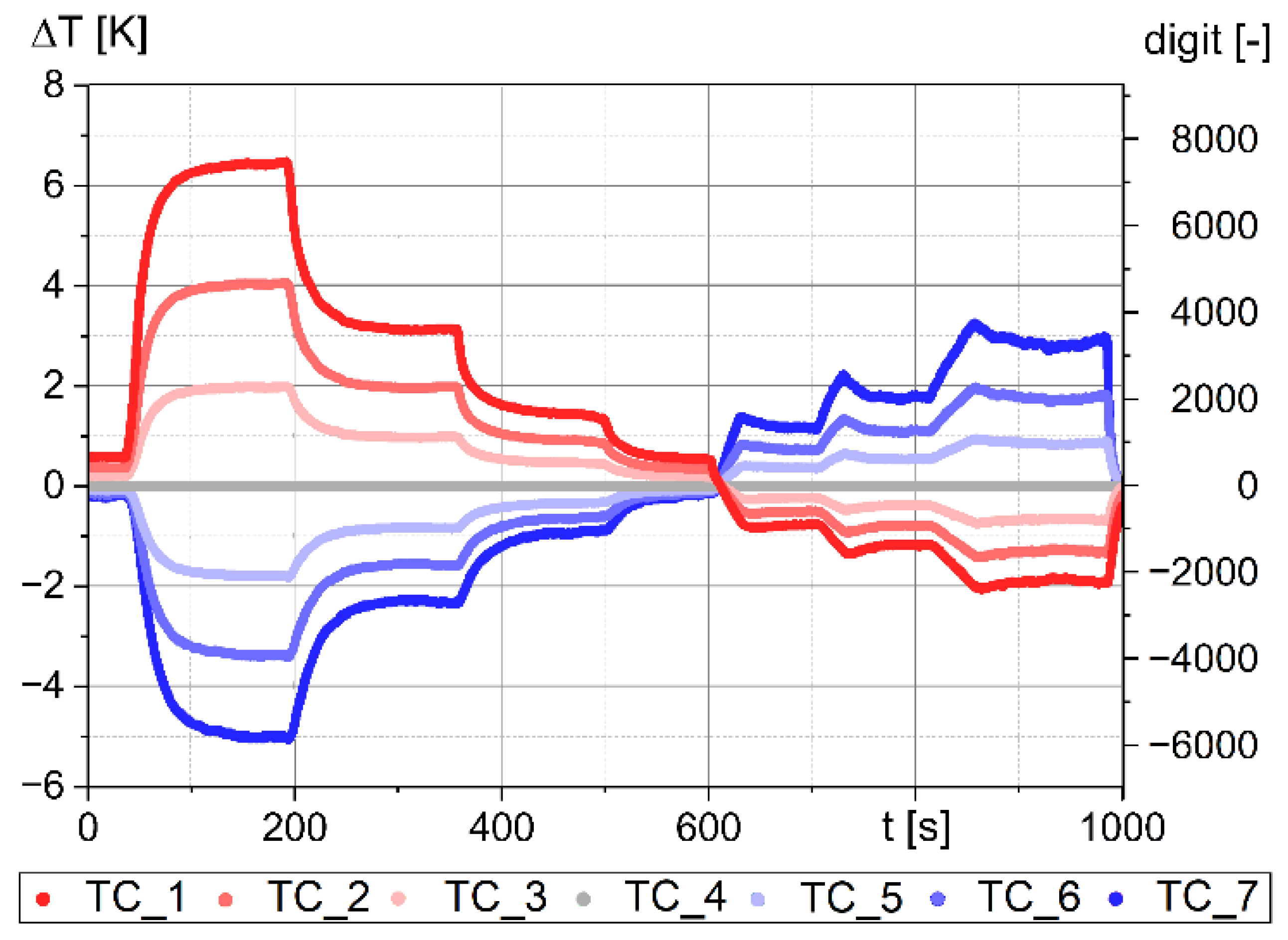
Figure 3.
Full-scale test rig of a steam turbine with focus on the side space, which was investigated [22,24].
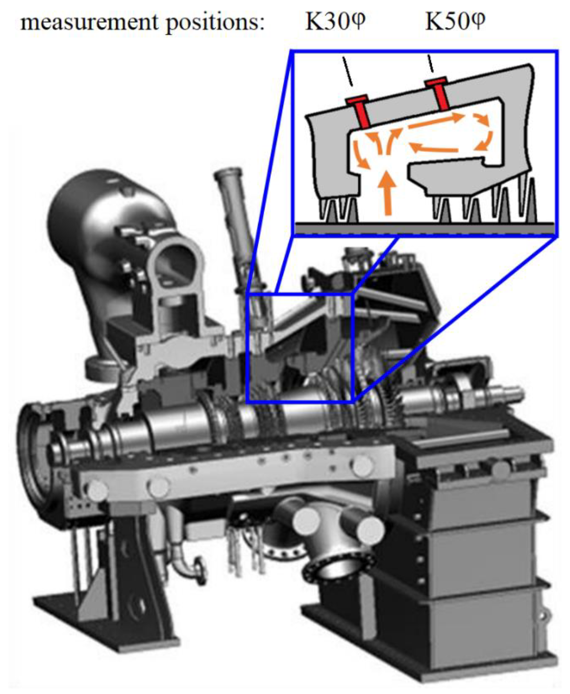
Figure 4.
Left: Individual adaptation of the sensor to the respective measuring position. Right: Boroscopic picture of the inside of the casing of the steam turbine after installation. The sensors were flush-mounted with the surface of the complex internal geometry. The light-coloured particles show corrosion effects in form of rust.
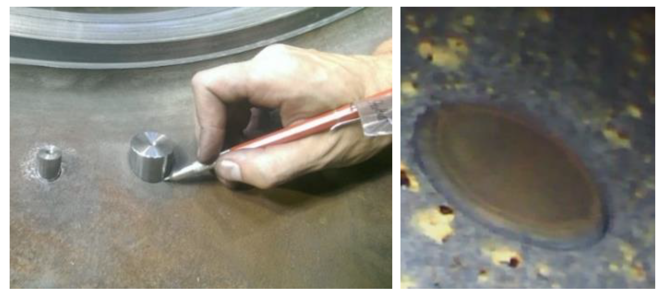
Figure 5.
Comparison of the different thermal resistances. Determination of the thermal influence of the sensor in relation to the original casing wall.
Figure 5.
Comparison of the different thermal resistances. Determination of the thermal influence of the sensor in relation to the original casing wall.
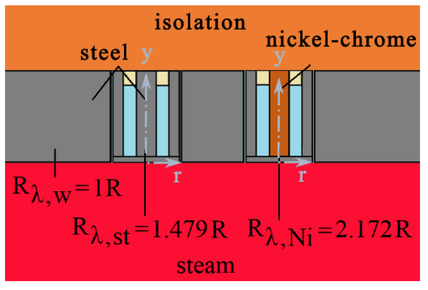
Figure 6.
Four solid and one fluid domain with different regions for various boundary conditions. A-fluid (side space), B-guide vane carrier 2 (IP) C-casing, D-guide vane carrier 3, E-exhaust steam casing. black line-heat transfer wall (HTW), blue line 9 (fluid-solid-interface).
Figure 6.
Four solid and one fluid domain with different regions for various boundary conditions. A-fluid (side space), B-guide vane carrier 2 (IP) C-casing, D-guide vane carrier 3, E-exhaust steam casing. black line-heat transfer wall (HTW), blue line 9 (fluid-solid-interface).
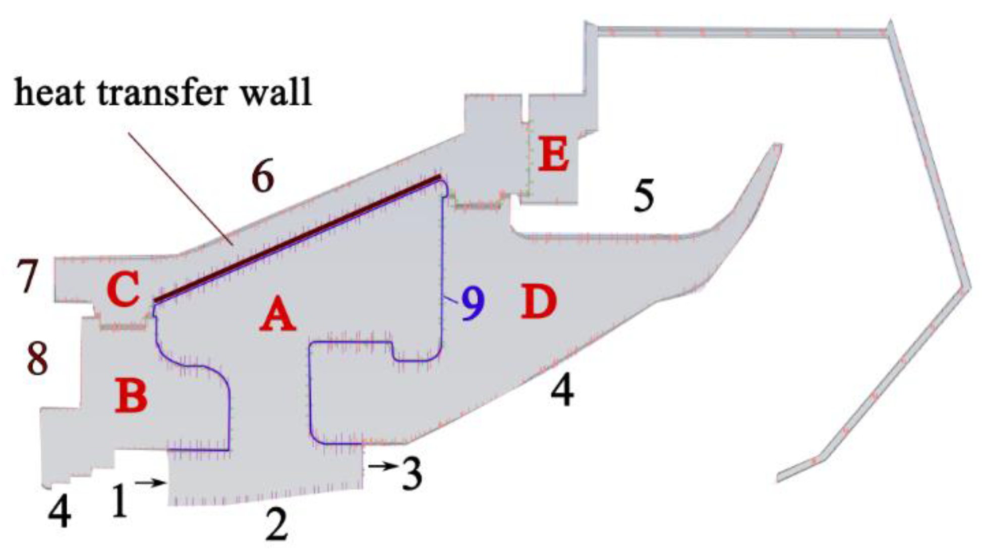
Figure 7.
Structured mesh with 1:1 interface of the fluid-solid-interface an inflation layers.
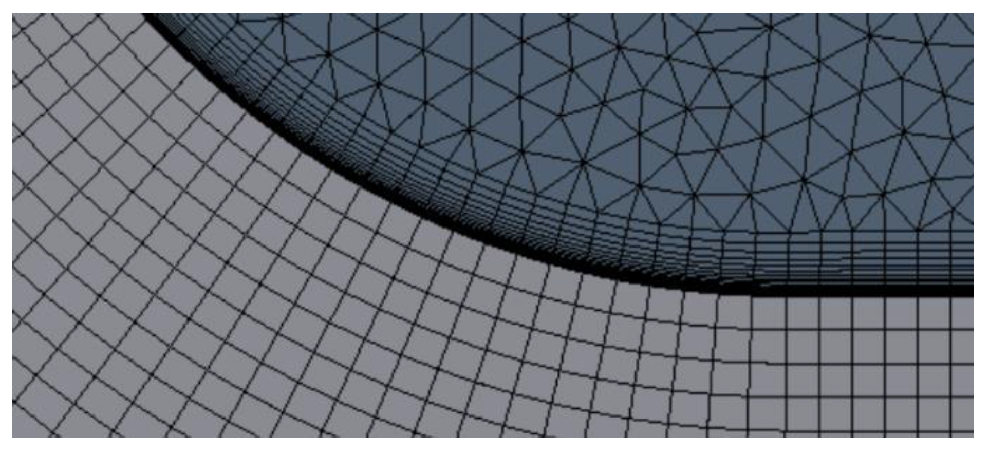
Figure 8.
The distribution of the temperature for the fluid and the solid domain is shown for different operation points.
Figure 8.
The distribution of the temperature for the fluid and the solid domain is shown for different operation points.
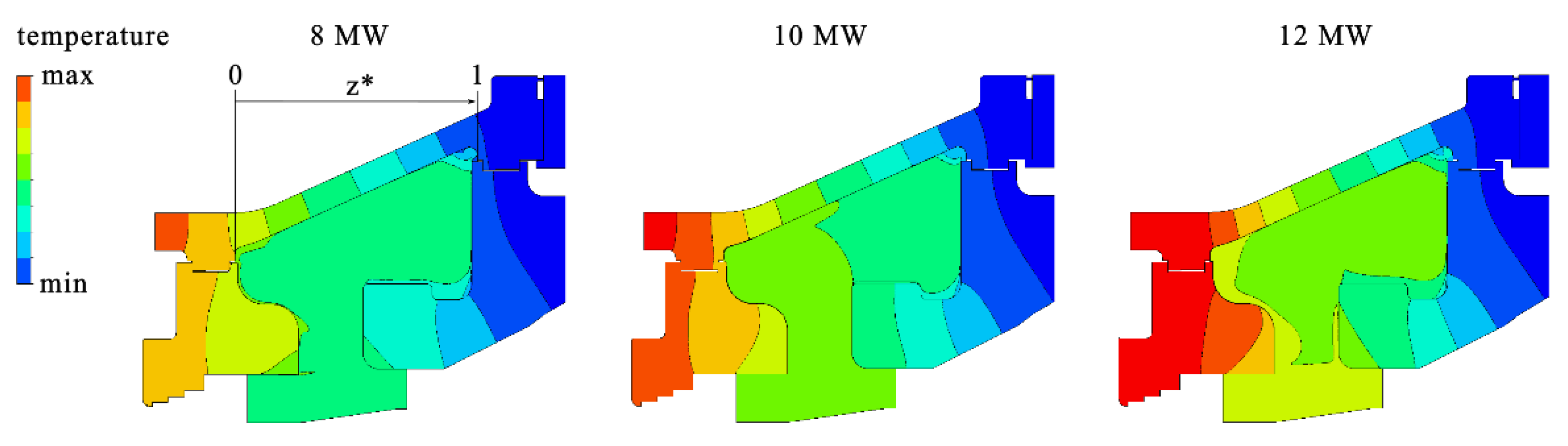
Figure 9.
Chart of temperature as a function of the dimensionsless axial coordinate z*.
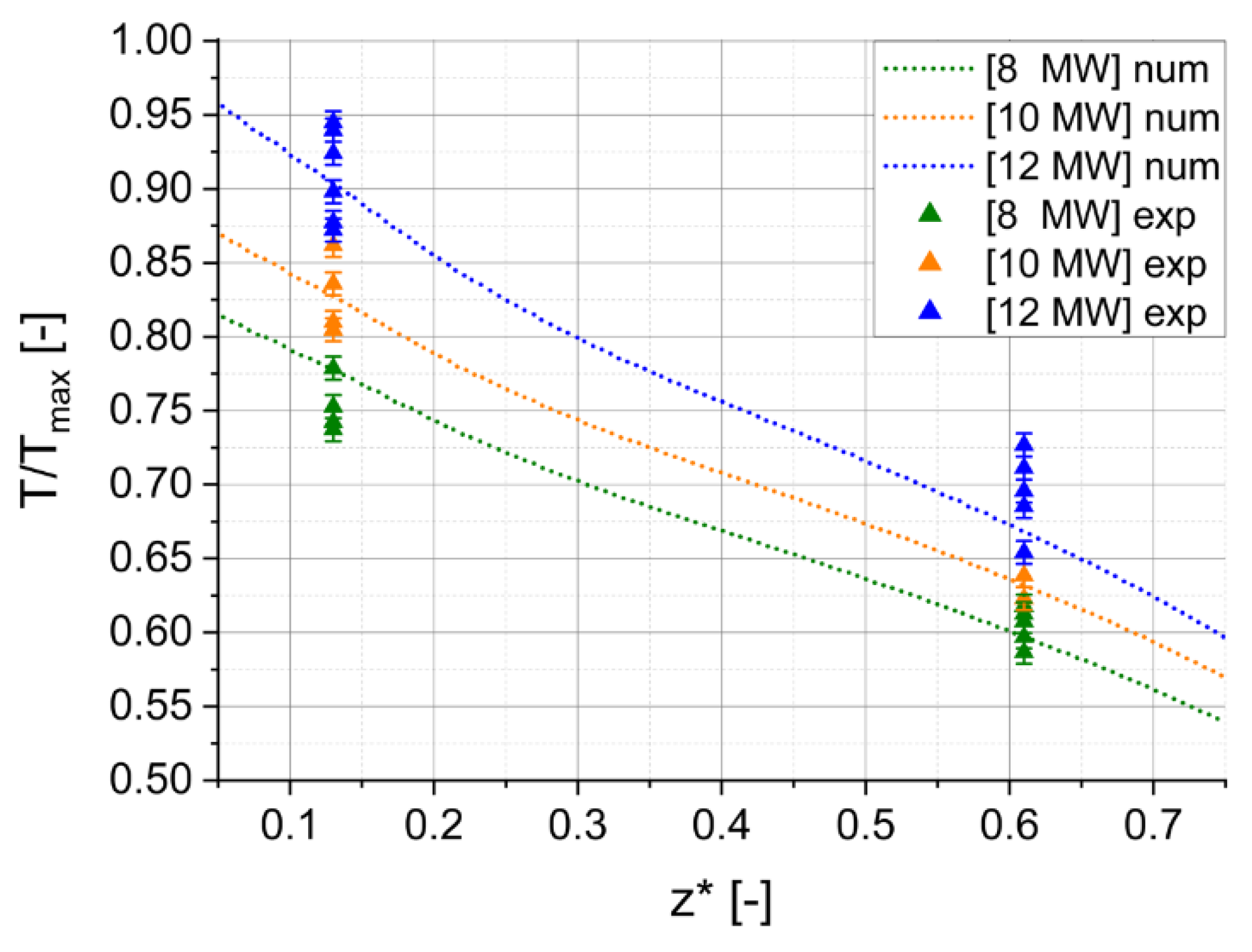
Figure 10.
Visualisation of streamlines – a mutiple vortex system with two dominating eddies (a, b) and other smaller ones (c, d) can be recognized. The radial velocity component is shown in colour. Red means positive radial velocity, blue the opposite.
Figure 10.
Visualisation of streamlines – a mutiple vortex system with two dominating eddies (a, b) and other smaller ones (c, d) can be recognized. The radial velocity component is shown in colour. Red means positive radial velocity, blue the opposite.
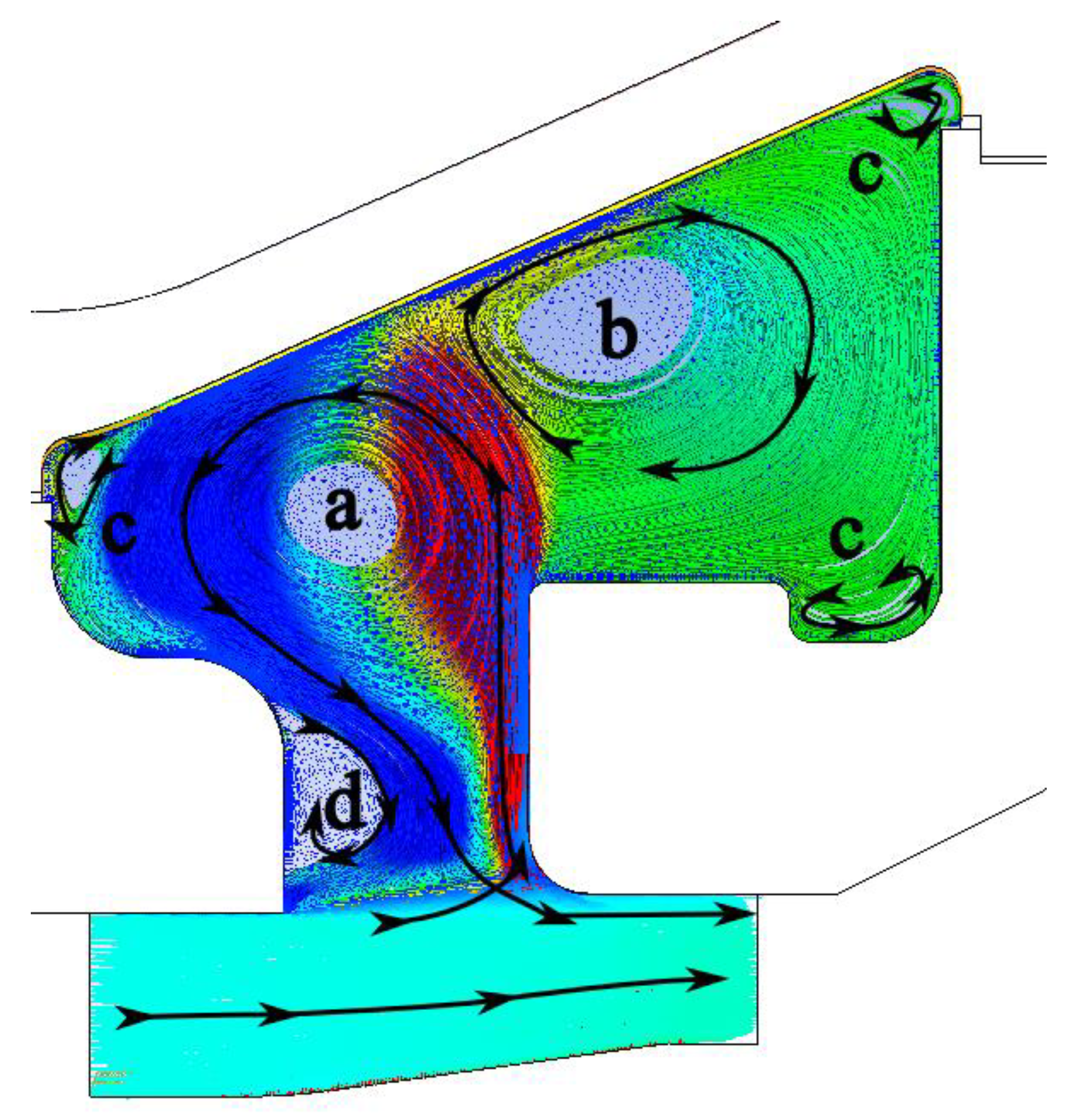
Figure 11.
Chart of heat flux as a function of the dimensionless axial coordinate
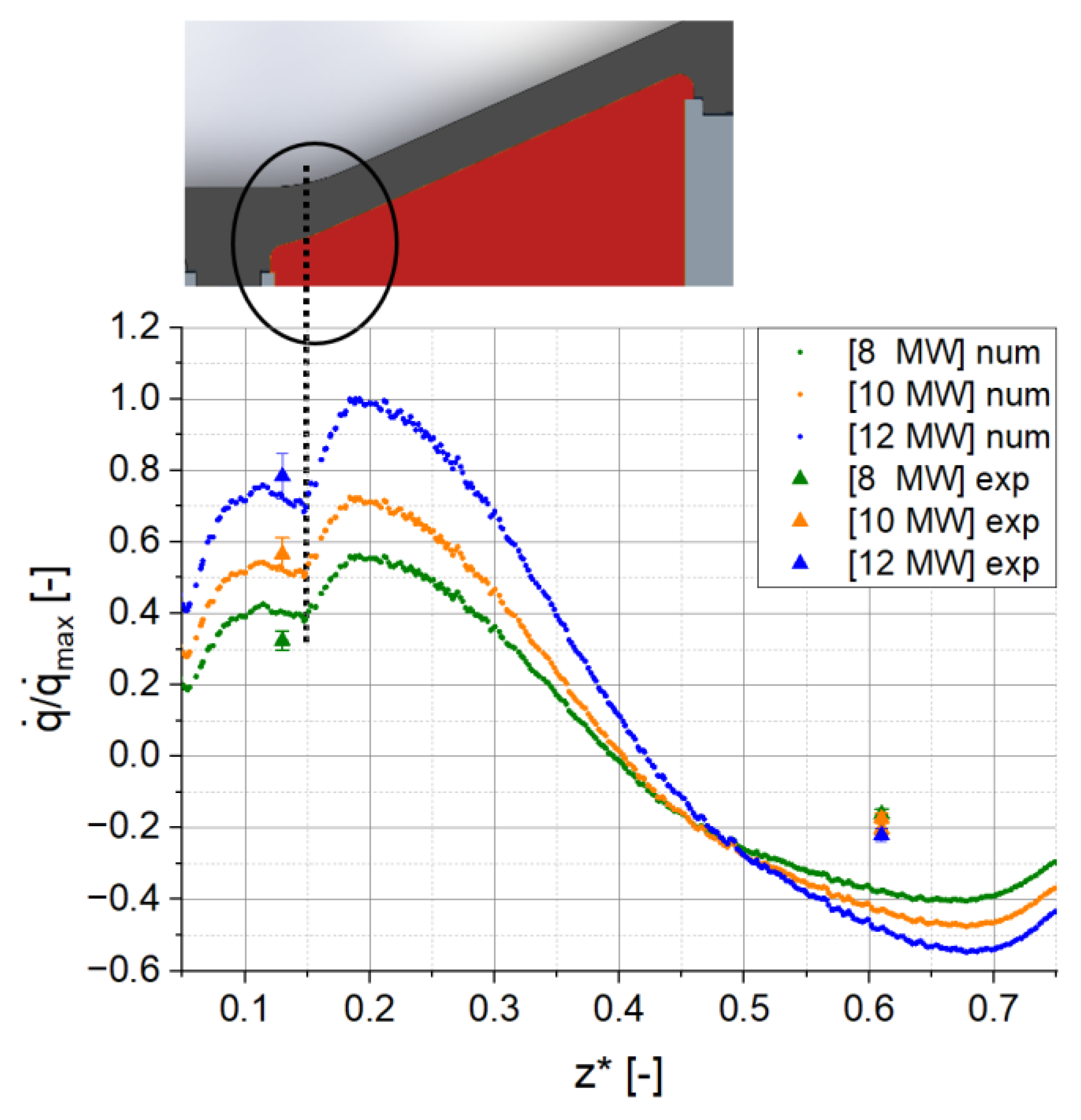
Figure 12.
Illustration of the temperature field of the numerical fluid and solid domain. Supplementary the heat affected zones were marked.
Figure 12.
Illustration of the temperature field of the numerical fluid and solid domain. Supplementary the heat affected zones were marked.
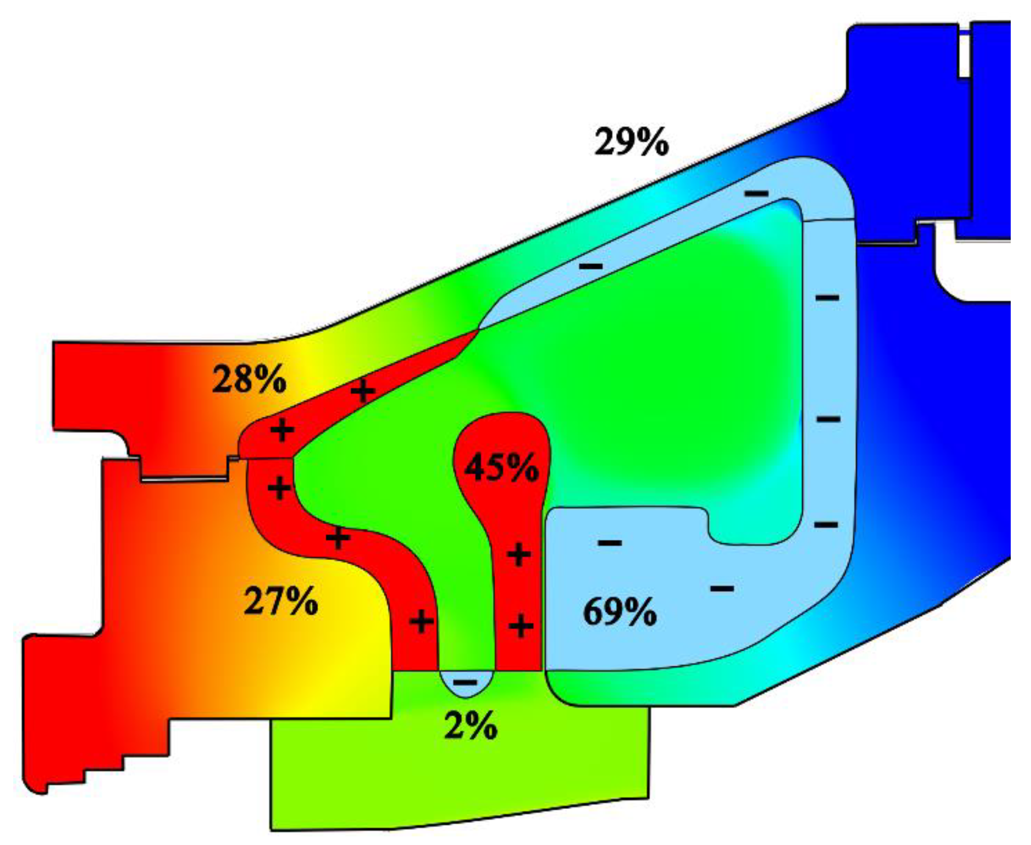
Figure 13.
Chart of heat transfer coefficient as a function of the dimensionless axial coordinate z*.
Figure 13.
Chart of heat transfer coefficient as a function of the dimensionless axial coordinate z*.
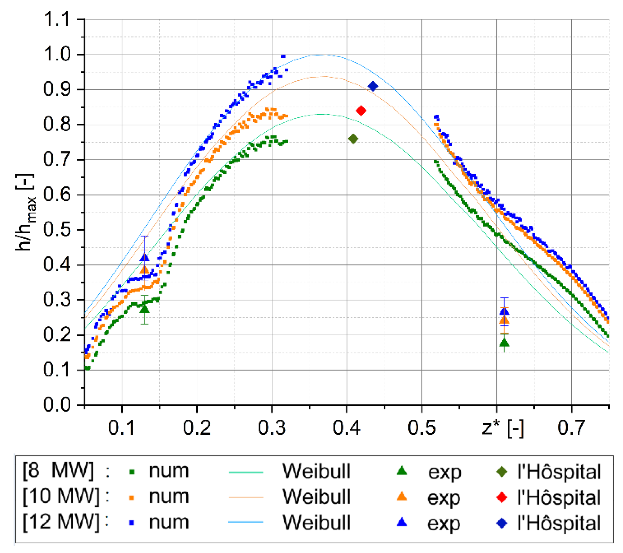
Figure 14.
Chart of the heat transfer coefficient as a function of power, compared to literature results [10,19].
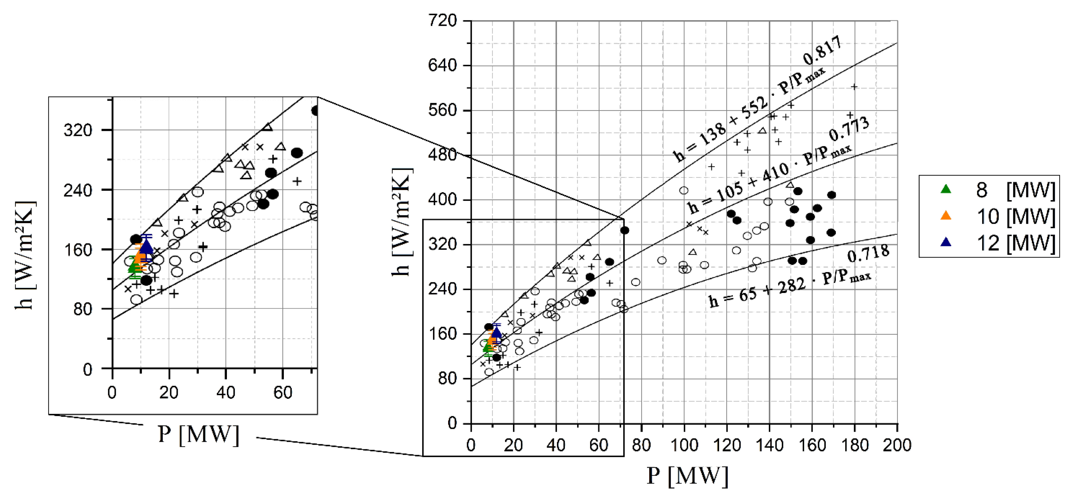

Table 1.
Comparison of heat flux measurements during steam turbine start-up, with and without adjustment factors.
Table 1.
Comparison of heat flux measurements during steam turbine start-up, with and without adjustment factors.
| K301 (steel) | K302 (NiCr) | K501 (steel) | K502 (NiCr) | |
|---|---|---|---|---|
| [24] | 20.88 | 14.42 | 21.55 | 14.56 |
| uncertainty analysis | 2.70 | 3.87 | 2.70 | 3.87 |
| consideration of the thermal influence of the sensor |
30.89 |
31.32 |
31.87 |
31.62 |
| relative deviation from the average (2σ)/% | 1.70 | 0.33 | 1.42 | 0.62 |
Table 2.
overview on grid parameter.
| mesh | nodes | scale | elements |
|---|---|---|---|
| 1 | 172 243 | - | 60 552 |
| 2 | 863 935 | 5,0 | 359 313 |
| 3 | 4 152 770 | 4,8 | 1 736 977 |
| 4 | 22 496 069 | 5,4 | 9 253 465 |
Table 3.
Definition of mesh regions, labelling and type of boundary conditions used.
| mesh region | designation | boundary condition |
|---|---|---|
| 1 | inlet | - dry steam (IAPWS) measured: - , , , |
| 2 | rotor | - adiabatic - no-slip-wall measured: - rotating wall |
| 3 | outlet | measrued: - |
| 4 | boundary flow passage | - adiabatic |
| 5 | exhaust steam casing | - h measured: T |
| 6 | ambient air | - h (represents also the isolation) measured:T |
| 7 | IP-casing | - Dirichlet; measured: |
| 8 | HP-IP-side space | - h measured:T |
| 9 | fluid-solid-interface | - 1:1 mesh - fluid-solid-interface |
Disclaimer/Publisher’s Note: The statements, opinions and data contained in all publications are solely those of the individual author(s) and contributor(s) and not of MDPI and/or the editor(s). MDPI and/or the editor(s) disclaim responsibility for any injury to people or property resulting from any ideas, methods, instructions or products referred to in the content. |
© 2025 by the authors. Licensee MDPI, Basel, Switzerland. This article is an open access article distributed under the terms and conditions of the Creative Commons Attribution (CC BY) license (https://creativecommons.org/licenses/by/4.0/).
Copyright: This open access article is published under a Creative Commons CC BY 4.0 license, which permit the free download, distribution, and reuse, provided that the author and preprint are cited in any reuse.


