
Submitted:
18 July 2025
Posted:
22 July 2025
You are already at the latest version
Abstract
Permeability is a fundamental petrophysical property that governs fluid flow and directly impacts production rates, reservoir management, and economic decisions in the oil and gas industry. Traditional measurement methods, such as core analysis and laboratory testing, are time-consuming, costly, and require specialized expertise. In response to these challenges, this study investigates the use of deep learning for permeability classification based on petrographic thin-section images from Brazilian pre-salt reservoirs. A custom classification scheme was developed in collaboration with a domain specialist to ensure practical relevance. Convolutional neural networks and Transformer-based architectures were evaluated, and despite the limited dataset size, the models demonstrated promising classification performance. The results indicate that image-based approaches can support permeability analysis, offering a potential complementary tool to traditional workflows. This study highlights the feasibility of integrating computer vision techniques into reservoir characterization, providing new perspectives for advancing petrophysical analysis.
Keywords:
petrophysics
; permeability
; reservoir characterization
; pre-salt
; machine learning
; deep learning
; ensemble
1. Introduction
Petrophysical properties, such as porosity, permeability, wettability, and fluid saturation, along with lithology definition, are fundamental in evaluating reservoir quality. Among these, porosity and permeability play central roles. Porosity denotes the volumetric proportion of pore space within a rock, which determines its capacity to store fluids such as oil, gas, or water. This makes it a key parameter for estimating the potential recoverable resources in a reservoir. Permeability, on the other hand, traditionally measured in millidarcies (, quantifies the ease with which fluids flow through the pore network, reflecting the reservoir’s productive potential. It is significantly influenced by the shapes, distribution, sizes, and connectivity of the pores [1]. Efficiently evaluating these properties is critical in the upstream segment of the oil and gas industry, as they directly impact the economic viability of reservoir development [2].
Several laboratory techniques are available for estimating porosity and permeability, including laboratory core analysis, Nuclear Magnetic Resonance (NMR), well logging, and micro-computed tomography (micro-CT) [1]. However, such methods are often time-consuming, costly, and reliant on specialized technical expertise [2]. In this context, machine learning has emerged as a compelling alternative, offering faster and more cost-effective solutions that often achieve performances comparable to or better than traditional approaches.
Machine learning models have been used across a wide range of oil and gas applications. Specifically, predictive models have utilized diverse input data sources, including well logs [3,4,5,6,7,8], NMR logs [9,10,11], and micro-CT images [12,13,14,15], to estimate porosity and permeability as continuous variables.
Fewer studies, however, have approached this problem as a classification task by discretizing porosity or permeability values into categorical intervals. In this regard, Silva et al. [16] and Freitas et al. [17] proposed classification-based frameworks for permeability using NMR relaxation data. Both adopted the same class intervals—}; }; }; and }—though based on different datasets. Silva et al. used a globally sourced carbonate dataset, while Freitas et al. focused on samples exclusively from the Brazilian pre-salt. The authors applied classical machine learning algorithms, including Random Forest (RF), k-Nearest Neighbors (KNN), Naïve Bayes (NB), and Sequential Minimal Optimization (SMO)—an SVM-based model. Silva et al. achieved their best results using SMO and RF, with an accuracy and weighted F-Measure of 85.9 %, after applying discretization and feature selection strategies. Freitas et al., by contrast, obtained 66 % accuracy using NB as the best-performing model, attributing the reduced performance to limited data diversity and sample size. Notably, Freitas et al. reported accuracy as their primary evaluation metric, while Silva et al. emphasized both accuracy and the weighted F-Measure1.
In a related study, Bedi and Toshniwal [18] developed a hybrid porosity classification model using seismic and well log data. They employed Empirical Mode Decomposition (EMD) for denoising and a Recurrent Neural Network (RNN) for classification, taking advantage of the temporal nature of the input signals. Porosity was discretized into two classes: low [0–0.6] and high [0.6–1], with the threshold selected to balance class distribution. Their model outperformed standard approaches including SVM, RF, and Artificial Neural Networks (ANN), achieving an average accuracy of 74 % and a G-mean2 of 0.80.
The present work adopts a similar classification-based strategy to predict discrete classes derived from permeability values using petrographic thin-section images. Although such images are typically used for lithological characterization, their application in inferring petrophysical properties remains largely unexplored. To date, no prior studies have applied deep learning models to classify permeability exclusively based on petrographic thin-section images from Brazilian pre-salt carbonate samples. This paper addresses this gap by evaluating the performance of well-established deep learning architectures, including Convolutional Neural Networks (CNNs) and Transformer-based models. The application of Transformer-based architectures in this context also constitutes a novel contribution to the field of reservoir characterization.
The remainder of this paper is organized as follows: the Materials and Methods section details the dataset and preprocessing steps used to adapt the images for deep learning, along with the anomaly detection strategy and the creation of permeability classes. It also introduces the evaluated deep learning architectures, training procedures, evaluation metrics, and the techniques adopted to address data imbalance. The Results and Discussion section presents the experimental findings and analyzes the performance of the proposed models. Finally, the Conclusions and Future Works section summarizes the main contributions and outlines potential directions for future research.
2. Materials and Methods
This section describes the procedures adopted to transform the original dataset into a format commonly used in image-based deep learning applications, including standardized input resolution and compatible data structures. It details the preprocessing steps, the creation of permeability-based classes, and the strategies employed to train, validate, and assess model generalization performance. Additionally, it outlines the techniques used to address class imbalance and presents the evaluation metrics adopted in this study.
2.1. The Dataset
The original dataset used in this research comprises 770 petrographic thin sections of carbonate samples from Brazilian pre-salt reservoirs. Each sample includes two high-resolution RGB photomicrographs: one acquired under plane-polarized light (PPL) and the other under cross-polarized light (XPL). Samples are annotated with porosity and permeability values obtained from laboratory analyses. The images appear in either rectangular or circular formats, depending on the type of rock cut (plug or plug-head).
2.1.1. Image Preprocessing
To ensure consistency and compatibility with deep learning models, a series of preprocessing steps were applied. First, all images were resized to 256 × 256 × 3 pixels. A central square crop was then used to reduce the impact of non-data regions commonly found between the thin section and the image borders, which are often present due to the variability in the shape of thin sections. Although some non-data areas remained, extensive experimentation throughout this work indicated that this cropping strategy was more effective than excessively aggressive approaches, which led to substantial data loss. Finally, all images were resized to 224 × 224 × 3 pixels to match the input size required by the pre-trained models. Figure 1 illustrates the preprocessing results.
2.1.2. Anomaly Detection
To identify and exclude potential outliers that could negatively impact model performance, anomaly detection was performed using an AutoEncoder [19] from the pyod [20] library with default parameters. A self-supervised learning strategy was employed by embedding the images into a latent space using a Vision Transformer (ViT) variant trained under the DINOv2 [21]. Reconstruction errors—differences between original and reconstructed images—were used to compute anomaly scores.
To maximize available information, an early fusion [22] strategy was employed by concatenating the corresponding PPL and XPL images along the channel dimension, resulting in a 256 × 256 × 6 tensor for each sample.
A domain specialist reviewed the outliers flagged by the AutoEncoder. Only the samples jointly identified as outliers by both the model and the specialist were removed. This process reduced the dataset by 16.23 %, resulting in a refined set of 645 samples. The overall workflow is illustrated in Figure 2.
2.1.3. Final Dataset and Class Creation
To provide a qualitative perspective on reservoir characterization, permeability values were discretized into four classes, defined in consultation with a domain expert, and based on preprocessing results (Table 1). Despite some differences in the intervals, this work adopted the same class names from Freitas et al. [17]. A scatter plot of permeability versus porosity is shown in Figure 3, where a logarithmic scale emphasizes the distinction between low and high permeability.
Although a strong log-linear correlation is observed between permeability and porosity, the dataset remains imbalanced. Therefore, specific strategies were required to mitigate potential model bias toward the majority classes. These techniques are described in Section 2.3.3, Section 2.3.4, and Section 2.3.5.
2.2. Deep Learning Architectures
To address the proposed classification task, several state-of-the-art deep learning models were selected, including both Convolutional Neural Networks (CNNs) and Transformer-based architectures. These models have consistently demonstrated strong performance across a wide range of computer vision tasks, such as classification, object detection, and semantic segmentation [23,24].
Deep learning architectures operate hierarchically: shallower layers tend to capture low-level patterns (e.g., edges and textures), whereas deeper layers progressively learn more abstract and semantic representations [25,26]. This layered feature extraction enables models to infer meaningful information directly from raw input data, reducing or eliminating the need for handcrafted features.
All models used in this study were sourced from the timm library, a well-established repository of pre-trained vision architectures [27]. They were initially trained on large-scale image classification benchmarks, either ImageNet-1k [28] or ImageNet-21k [29], and subsequently fine-tuned on the thin-section dataset available in the present research.
2.2.1. Residual Network
The Residual Network (ResNet) [30,31] introduced identity-based skip connections, which enable the flow of gradients through deep layers by allowing the input to bypass intermediate transformations. These residual connections mitigate the vanishing gradient problem, facilitating the training of very deep networks.
This work adopted a 50-layer ResNet architecture trained on ImageNet-1k using an improved training configuration that includes stronger data augmentation and regularization techniques. This setup enhances generalization, especially when fine-tuned on domain-specific datasets such as petrographic images.
2.2.2. Densely Connected Network
DenseNet [32] enhances feature reuse and gradient flow by connecting each layer to all preceding layers via feature map concatenation. Unlike ResNet, which adds feature maps, DenseNet explicitly preserves and reuses learned representations throughout the network, resulting in improved parameter efficiency and learning dynamics.
In this study, a 201-layer DenseNet architecture was employed. This variant was originally trained on ImageNet-1k and is known for its favorable trade-off between depth, performance, and computational cost, particularly effective in tasks involving limited training data.
2.2.3. Vision Transformer
The Vision Transformer (ViT) [33] marked a paradigm shift in visual modeling by applying the Transformer architecture—originally designed for natural language processing [34]—to image classification. In ViT, each image is divided into non-overlapping patches, which are linearly embedded and treated as input tokens to a standard Transformer encoder. Global self-attention mechanisms enable the model to capture long-range dependencies across the image.
This research adopted a base-sized ViT model with 8 × 8 patch size. It was pre-trained on ImageNet-21k using advanced augmentation and regularization strategies and later fine-tuned on ImageNet-1k. This combination has demonstrated excellent transfer learning capacity, making it well-suited for specialized applications like petrographic image analysis.
2.2.4. Swin Transformer
The Swin Transformer [35] presents a hierarchical alternative to ViT by computing self-attention within shifted local windows rather than globally. These windows shift across layers, enabling the model to capture both local and global context in a computationally efficient manner. The Swin architecture supports scalability to high-resolution images while maintaining strong performance.
The adopted variant in this study is a large-scale Swin Transformer, originally pre-trained on ImageNet-21k using multi-scale augmentation strategies. It uses 4 × 4 patch sizes and 7 × 7 attention windows, offering an effective balance between detailed local features and long-range dependencies.
2.3. Training
2.3.1. Cross-Validation
The dataset was split into 80 % for training and 20 % for testing. Due to class imbalance, the split was stratified to preserve the original class distribution in both subsets. The test set was reserved exclusively for assessing the model’s generalization to unseen data.
To ensure robust learning and reduce overfitting, five-fold cross-validation was performed. In this approach, the training data are divided into five equal partitions, or folds. At each iteration, one fold is used for validation, while the remaining four folds are used for training. This process is repeated five times so that every sample in the training set is used once for validation. Final performance is reported as the average across all five folds. Figure 4 presents the cross-validation scheme.
This procedure provides a reliable estimate of model performance and supports model selection. The test set remained untouched until the final evaluation stage.
2.3.2. Data Augmentation
To enhance data diversity and reduce overfitting, this study employed RandAugment [36], a policy-based data augmentation technique. RandAugment applies a random combination of transformations controlled by two user-defined parameters: the number of transformations and their magnitude.
Unlike conventional augmentation methods, RandAugment does not require manually predefined augmentation policies. In this work, the configuration was selected based on hyperparameter tuning, allowing both geometric and appearance-based transformations to be applied. These may include rotation, flipping, color distortion, contrast adjustment, or minor geometric warping.
Despite the risk of slightly altering subtle features in thin-section images, RandAugment improved validation performance, indicating that the introduced variations helped the model generalize to unseen patterns.
2.3.3. Class Weighting
Another commonly used strategy to handle imbalanced datasets is class weighting, where the loss function is adjusted to penalize misclassifications from underrepresented classes more heavily.
In this study, class weights were computed as the inverse of the class frequencies and normalized to sum to 1:
where:
- N is the total number of training samples,
- C is the number of classes,
- is the number of samples in class c.
This approach is supported by most modern deep learning frameworks, such as PyTorch [37], and was evaluated as part of this work. It was incorporated into the final training pipeline only when it contributed positively to performance metrics such as the macro F1-score.
2.3.4. Batch-wise Class Balancing
In addition to loss-based methods, this work also explored a data-level balancing strategy known as batch-wise class balancing. This method ensures that each training batch contains a uniform distribution of classes by oversampling minority class instances.
During training, samples from underrepresented classes were randomly duplicated so that all classes were equally represented in each batch. This balanced composition can help the model avoid becoming biased toward majority classes, particularly in the early stages of training.
However, as with other imbalance mitigation strategies, batch-wise balancing was included in the final training configuration only when it demonstrably improved class-wise generalization or validation metrics.
2.3.5. Focal Loss
Standard loss functions such as categorical cross-entropy often struggle in imbalanced classification scenarios, as they are dominated by majority classes. To address this issue, the Focal Loss [38] was investigated as a potential alternative to enhance learning from hard-to-classify (typically minority class) samples.
Focal Loss modifies the cross-entropy loss by applying a modulating factor , where is the predicted probability for the true class, and is the focusing parameter. This formulation down-weights well-classified examples, enabling the model to concentrate more on challenging samples. As shown in Figure 5, increasing progressively reduces the loss contribution from well-classified examples, which helps balance the influence of majority and minority classes.
where:
- is the predicted probability for the correct class,
- is a positive scalar that controls the strength of the focusing effect.
This technique was tested as part of the training strategy and retained only when it resulted in measurable improvements in model generalization, particularly with respect to minority classes.
2.3.6. Fine-Tuning
To adapt the pre-trained models to the classification task in this study, a fine-tuning strategy was employed. Specifically, the original classification head was replaced by a new fully connected layer tailored to the four permeability-based classes defined in this work.
This strategy allows the models to retain the rich, low-level, and mid-level visual representations learned during large-scale pre-training while adjusting their final layers to the domain-specific characteristics of petrographic thin-section images. Fine-tuning is especially beneficial when dealing with relatively small datasets, as it significantly improves convergence and generalization.
As shown in Figure 6, an early fusion [22] approach was applied during input preparation. Each sample’s pair of images—one acquired under plane-polarized light (PPL) and the other under cross-polarized light (XPL)—was concatenated along the channel dimension, yielding a 6-channel tensor of shape . This fused representation was used as input for all models.
All models were trained using the Adam optimizer [39], which combines the advantages of adaptive learning rates and momentum. A cosine annealing schedule [40] was applied to gradually reduce the learning rate throughout training, helping to refine the model in later stages.
Early stopping was also implemented, terminating the training process if the validation performance failed to improve after a predefined number of epochs. This helped reduce unnecessary computation and minimized the risk of overfitting. Hyperparameters used in the fine-tuning process are detailed in the Results and Discussion section.
2.3.7. Evaluation Metrics
Given the imbalanced nature of the dataset, classification accuracy alone was deemed insufficient for evaluating model performance. Accuracy can be misleading in imbalanced scenarios, as it may reflect strong performance on majority classes while masking poor performance on minority classes.
Instead, the primary metric adopted in this study was the macro F1-score, which balances precision and recall. For binary classification, the F1-score is defined as:
Where:
- TP (True Positives): correct predictions of the positive class;
- FP (False Positives): incorrect predictions of the positive class;
- FN (False Negatives): missed predictions of the positive class.
For multi-class classification, the F1-score is extended using the macro F1-score. This metric calculates the F1-score independently for each class and then takes the unweighted mean across all classes, giving equal importance to each one:
Where:
- C is the number of classes,
- is the F1-score for class i.
The macro F1-score ensures a fair evaluation across all classes, which is particularly important when dealing with minority classes in imbalanced datasets such as the one used in this research.
2.3.8. Ensemble Prediction Strategy
In addition to individual fold evaluations, this study employed an ensemble prediction strategy to aggregate the outputs of multiple models. Specifically, a soft voting ensemble [41] was implemented using the models trained during the five-fold cross-validation procedure.
Each model produced class logits for the test set, which were subsequently transformed into score vectors via the softmax function. These scores lie within the interval [0, 1] and sum to 1 per sample. In this study, the resulting values are treated as confidence scores, reflecting the relative belief of each model in each class.
The final prediction was obtained by averaging the softmax scores across the five models and selecting the class with the highest mean score. This method represents a consensus-based voting approach that incorporates the confidence levels of each base model.
Formally, let represent the softmax score vector for sample i as predicted by model j. The ensemble score is computed as:
where M is the number of models (in this case, five). The final class prediction is given by:
This technique corresponds to an independent soft voting ensemble, as described in the ensemble learning literature [41]. It enables the integration of diverse and independently trained models, enhancing robustness and reducing variance. The average macro F1-score of the ensemble was compared with that of the individual models, confirming its positive impact on overall performance.
3. Results and Discussion
This section presents the experimental results obtained by the fine-tuned pre-trained models, as well as the hyperparameters selected during optimization. The Optuna [42] library was used for this purpose due to its seamless integration with PyTorch and its support for advanced sampling strategies.
A consistent search space was defined for all models, including:
- Learning rate: logarithmic range between and ;
- Number of transformations applied by RandAugment: from 2 to 4;
- Transformation magnitude applied by RandAugment: from 3 to 15.
Throughout the research, including all stages before and after hyperparameter tuning, hundreds of training experiments were conducted. Across these iterations, no significant improvements were observed when using additional regularization techniques. Therefore, parameters such as weight decay, dropout, or the use of AdamW [43]—which relies more heavily on regularization than Adam—were excluded from the final tuning configuration. Nevertheless, the search space adopted proved suitable for the task.
To optimize both validation loss and macro F1-score, a multi-objective approach was adopted. The NSGAIISampler [44] from Optuna was chosen due to its effectiveness in handling such objectives. Each model underwent up to 100 trials or a maximum of 12 hours of optimization. Training was limited to 300 epochs using a batch size of 32, with early stopping applied using a patience of 15 epochs. A fixed random seed ensured reproducibility. Learning rate scheduling followed a cosine annealing strategy with warm restarts [40], using default settings except for , which was set to 103. Table 2 summarizes the best hyperparameters selected for each architecture.
Following hyperparameter optimization, each model was retrained using its respective best configuration, maintaining the same setup (e.g., batch size, early stopping, learning rate scheduler, value). Class imbalance mitigation strategies—including Focal Loss, class weighting, and batch-wise class balancing—were tested individually, and only those that provided measurable improvements were included in the final configuration. In some cases, further fine-tuning, such as unfreezing an earlier layer or adding an extra fully connected layer to the classification head, yielded additional performance gains.
All models were trained using five-fold cross-validation, and this setup remained unchanged during final training. Model evaluation was performed on the held-out test set. Each fold’s model generated predictions for the test set, resulting in five independent evaluation runs. The final reported score is the average macro F1-score across all folds, as shown in Table 3. In addition, Figure 7 shows the training and validation curves for the ViT-B/8 model, which achieved the best performance.
An ensemble strategy was also implemented using soft voting, where the logits from each fold’s model were averaged (after softmax application), and the final prediction was obtained by selecting the class with the highest mean score. Table 4 presents the classification results per class for each model, including precision, recall, and F1-score, as well as overall accuracy and macro F1-score. Furthermore, Figure 8 presents the confusion matrices for all ensemble models evaluated on the test set.
Additionally, Figure 9 offers a qualitative perspective on the ViT-B/8 ensemble model predictions by relating porosity and permeability values in the test set. In particular, misclassified samples from the High class tend to cluster near class boundaries, emphasizing the difficulty of assigning correct labels to samples that lie close to decision thresholds. Although a monotonic trend between porosity and permeability is evident, overlapping distributions near these boundaries increase the likelihood of errors. This behavior is consistent with the confusion matrices shown in Figure 8, which also reflect the reduced classification performance for the High class.
Compared to previous works, such as Silva et al. [16] and Freitas et al. [17], two aspects are worth highlighting. First, although the class intervals are not identical, the final two permeability ranges are equivalent. Second, this study relied exclusively on image data, excluding porosity and NMR relaxation data, which were used as input features in both Silva et al. and Freitas et al. This distinction is particularly relevant, as the models in the previous studies were trained on petrophysical measurements that provide direct physical proxies for permeability, whereas this work focuses solely on thin-section images.
Although the results in this study did not surpass those of Silva et al., who achieved higher performance using NMR data and feature selection strategies, they did outperform the results reported by Freitas et al., who also worked with Brazilian pre-salt samples. It is important to note that the comparison is not strictly direct due to differences in the types of input data and modeling approaches. Table 5 presents the comparative accuracies.
The underperformance of minority classes—particularly the High class—can be attributed to multiple factors: (i) the intrinsic heterogeneity of carbonate rocks from the Brazilian pre-salt; (ii) the three-dimensional nature of permeability versus the two-dimensional character of thin-section images; (iii) the sparse and scattered distribution of samples from the High class in feature space; and (iv) the relatively small dataset size.
Despite these challenges, the results confirm the feasibility of using thin-section images for permeability classification through deep learning. Transformer-based models, especially ViT, have demonstrated competitive performance and represent a promising direction for future research in image-based reservoir characterization.
4. Conclusions and Future Works
This study proposed a novel approach for classifying permeability intervals directly from petrographic thin-section images using deep learning models. Both Convolutional Neural Networks (CNNs) and Transformer-based architectures were explored, with the latter demonstrating superior performance across most evaluation metrics. In particular, the ViT-B/8 model achieved the best overall results, supported by careful hyperparameter tuning, data augmentation, and ensemble learning strategies.
Unlike traditional approaches that rely on numerical well logs or NMR measurements, this work demonstrated the feasibility of using only 2D petrographic imagery for permeability classification. This expands the range of data sources available for reservoir characterization, especially in scenarios where core or log data are limited or unavailable.
When compared to prior studies, the proposed method outperformed the approach developed by Freitas et al., which also focused on Brazilian pre-salt samples. Although the results of Silva et al. remain superior in terms of accuracy, it is important to note that their model was trained on a globally sourced dataset with greater variability and incorporated NMR data as input. The performance achieved in this work—without relying on porosity measurements or laboratory-acquired wellbore wireline data—represents a significant advancement in the image-based classification of petrophysical properties.
Future research could investigate multi-objective learning strategies to predict permeability and porosity simultaneously, leveraging their intrinsic relationship. Hybrid architectures that combine convolutional neural networks and Transformer-based models may further enhance the representational power of deep learning frameworks. Additionally, incorporating uncertainty quantification methods could improve the assessment of model reliability and support greater interpretability in practical reservoir applications.
An additional research direction could involve multimodal learning approaches that integrate petrographic images, NMR measurements, and structured well-log data. By combining the complementary strengths of these diverse data sources, such models may improve prediction accuracy, reduce uncertainty, and enable more robust reservoir characterization, particularly in data-limited scenarios.
Author Contributions
Conceptualization, G.G.A., C.R.H.B., and M.R.K.; methodology, G.G.A., C.R.H.B., and M.R.K.; software, G.G.A.; validation, G.G.A., C.R.H.B., M.R.K., A.C., M.R.B., and M.A.C.P.; formal analysis, G.G.A., C.R.H.B., and M.R.K.; investigation, G.G.A., C.R.H.B., and M.R.K.; resources, M.A.C.P.; data curation, G.G.A., A.C., and M.R.B.; writing—original draft preparation, G.G.A.; writing—review, G.G.A., C.R.H.B., M.R.K., A.C., M.R.B., and M.A.C.P.; writing—editing, G.G.A.; visualization, G.G.A.; supervision, C.R.H.B. and M.R.K.; project administration, M.R.K. and M.A.C.P.; funding acquisition, not applicable. All authors have read and agreed to the published version of the manuscript.
Funding
The authors thank the financial support by the Brazilian funding agencies CNPq, FINEP, and FAPERJ. This work was financed in part by Coordenação de Aperfeiçoamento de Pessoal de Nível Superior—Brasil (CAPES)—Finance Code 001.
Data Availability Statement
The data and source code used in this study are not publicly available due to confidentiality agreements with Petróleo Brasileiro S.A. (Petrobras). Access to these resources is restricted and was provided only for academic research purposes under a confidentiality agreement.
Acknowledgments
The authors are grateful to Alexandre Sanchetta and Vitor Bento de Sousa, researchers at the Laboratório de Inteligência Computacional Aplicada (ICA) at PUC-Rio, for their valuable support and contributions to this project. The authors also thank Bernardo Coutinho Camilo dos Santos and Thais Fernandes de Matos from CENPES (Petrobras) for providing the necessary data access and support to conduct this research.
Conflicts of Interest
The authors declare no conflicts of interest.
References
- Schön, J. Physical properties of rocks: a workbook; Number 8 in Handbook of petroleum exploration and production, Elsevier: Amsterdam ; Boston, 2011. OCLC: ocn751711883.
- Lawal, A.; Yang, Y.; He, H.; Baisa, N.L. Machine Learning in Oil and Gas Exploration: A Review. IEEE Access 2024, 12, 19035–19058. [Google Scholar] [CrossRef]
- Ben-Awuah, J.; Padmanabhan, E. An enhanced approach to predict permeability in reservoir sandstones using artificial neural networks (ANN). Arabian Journal of Geosciences 2017, 10, 1–15. [Google Scholar] [CrossRef]
- Huang, Z.H.; Shimeld, J.; Williamson, M.; Katsube, J. Permeability prediction with artificial neural network modeling in the Venture gas field, offshore eastern Canada. GEOPHYSICS 1996, 61, 422–436. [Google Scholar] [CrossRef]
- Helle, H.B.; Bhatt, A.; Ursin, B. Porosity and permeability prediction from wireline logs using artificial neural networks: a North Sea case study. GEOPHYSICAL PROSPECTING 2001, 49, 431–444. [Google Scholar] [CrossRef]
- Liu, J.J.; Liu, J.C. Permeability Predictions for Tight Sandstone Reservoir Using Explainable Machine Learning and Particle Swarm Optimization. Geofluids 2022, 2022, 1–15. [Google Scholar] [CrossRef]
- Zhao, X.; Chen, X.; Huang, Q.; Lan, Z.; Wang, X.; Yao, G. Logging-data-driven permeability prediction in low-permeable sandstones based on machine learning with pattern visualization: A case study in Wenchang A Sag, Pearl River Mouth Basin. Journal of Petroleum Science and Engineering 2022, 214, 110517. [Google Scholar] [CrossRef]
- Matinkia, M.; Hashami, R.; Mehrad, M.; Hajsaeedi, M.R.; Velayati, A. Prediction of permeability from well logs using a new hybrid machine learning algorithm. Petroleum 2023, 9, 108–123. [Google Scholar] [CrossRef]
- Masroor, M.; Emami Niri, M.; Rajabi-Ghozloo, A.H.; Sharifinasab, M.H.; Sajjadi, M. Application of machine and deep learning techniques to estimate NMR-derived permeability from conventional well logs and artificial 2D feature maps. JOURNAL OF PETROLEUM EXPLORATION AND PRODUCTION TECHNOLOGY 2022, 12, 2937–2953. [Google Scholar] [CrossRef]
- Tariq, Z.; Gudala, M.; Yan, B.; Sun, S.; Mahmoud, M. A fast method to infer Nuclear Magnetic Resonance based effective porosity in carbonate rocks using machine learning techniques. GEOENERGY SCIENCE AND ENGINEERING 2023, 222, 211333. [Google Scholar] [CrossRef]
- Zhao, J.; Wang, Q.; Rong, W.; Zeng, J.; Ren, Y.; Chen, H. Permeability Prediction of Carbonate Reservoir Based on Nuclear Magnetic Resonance (NMR) Logging and Machine Learning. ENERGIES 2024, 17, 1458. [Google Scholar] [CrossRef]
- Araya-Polo, M.; Alpak, F.O.; Hunter, S.; Hofmann, R.; Saxena, N. Deep learning-driven permeability estimation from 2D images. COMPUTATIONAL GEOSCIENCES 2020, 24, 571–580. [Google Scholar] [CrossRef]
- Tembely, M.; AlSumaiti, A.M.; Alameri, W.S. Machine and deep learning for estimating the permeability of complex carbonate rock from X-ray micro-computed tomography. ENERGY REPORTS 2021, 7, 1460–1472. [Google Scholar] [CrossRef]
- dos Anjos, C.E.M.; de Matos, T.F.; Avila, M.R.V.; Fernandes, J.d.C.V.; Surmas, R.; Evsukoff, A.G. Permeability estimation on raw micro-CT of carbonate rock samples using deep learning. GEOENERGY SCIENCE AND ENGINEERING 2023, 222, 211335. [Google Scholar] [CrossRef]
- Mohyeddini, A.; Rasaei, M. Calculating porosity and permeability from synthetic micro-CT scan images based on a hybrid artificial intelligence. Canadian Journal of Chemical Engineering 2023, 101, 6591–6612. [Google Scholar] [CrossRef]
- da Silva, P.N.; Goncalves, E.C.; Rios, E.H.; Muhammad, A.; Moss, A.; Pritchard, T.; Glassborow, B.; Plastino, A.; de Vasconcellos Azeredo, R.B. Automatic classification of carbonate rocks permeability from 1H NMR relaxation data. EXPERT SYSTEMS WITH APPLICATIONS 2015, 42, 4299–4309. [Google Scholar] [CrossRef]
- Favacho de Freitas, K.L.; da Silva, P.N.; Faria, B.M.; Goncalves, E.C.; Rios, E.H.; Nobre-Lopes, J.; Rabe, C.; Plastino, A.; de Vasconcelos Azeredo, R.B. A data mining approach for automatic classification of rock permeability. JOURNAL OF APPLIED GEOPHYSICS 2022, 196, 104514. [Google Scholar] [CrossRef]
- Bedi, J.; Toshniwal, D. Features denoising-based learning for porosity classification. NEURAL COMPUTING & APPLICATIONS 2020, 32, 16519–16532. [Google Scholar] [CrossRef]
- A comprehensive survey on design and application of autoencoder in deep learning. Applied Soft Computing 2023, 138, 110176. [CrossRef]
- Zhao, Y.; Nasrullah, Z.; Li, Z. PyOD: A Python Toolbox for Scalable Outlier Detection. JOURNAL OF MACHINE LEARNING RESEARCH 2019, 20, 96. [Google Scholar]
- Oquab, M.; Darcet, T.; Moutakanni, T.; Vo, H.; Szafraniec, M.; Khalidov, V.; Fernandez, P.; Haziza, D.; Massa, F.; El-Nouby, A.; et al. DINOv2: Learning Robust Visual Features without Supervision. arXiv 2024. [Google Scholar] [CrossRef]
- Zhao, F.; Zhang, C.; Geng, B. Deep Multimodal Data Fusion. ACM Comput. Surv. 2024, 56, 216–1. [Google Scholar] [CrossRef]
- LeCun, Y.; Bengio, Y.; Hinton, G. Deep learning. NATURE 2015, 521, 436–444. [Google Scholar] [CrossRef] [PubMed]
- Bengio, Y.; Lecun, Y.; Hinton, G. Deep Learning for AI. COMMUNICATIONS OF THE ACM 2021, 64, 58–65. [Google Scholar] [CrossRef]
- Ballard, D.H.; Brown, C.M. Computer Vision, 1st ed.; Prentice Hall Professional Technical Reference, 1982.
- Stockman, G.; Shapiro, L.G. Computer Vision, 1st ed.; Prentice Hall PTR: USA, 2001. [Google Scholar]
- Wightman, R. PyTorch Image Models, 2025. [CrossRef]
- Russakovsky, O.; Deng, J.; Su, H.; Krause, J.; Satheesh, S.; Ma, S.; Huang, Z.; Karpathy, A.; Khosla, A.; Bernstein, M.; et al. ImageNet Large Scale Visual Recognition Challenge. arXiv 2015, arXiv:1409.0575. [Google Scholar] [CrossRef]
- Ridnik, T.; Ben-Baruch, E.; Noy, A.; Zelnik-Manor, L. ImageNet-21K Pretraining for the Masses. arXiv 2021, arXiv:2104.10972. [Google Scholar] [CrossRef]
- He, K.; Zhang, X.; Ren, S.; Sun, J. Deep Residual Learning for Image Recognition. arXiv 2015. [Google Scholar] [CrossRef]
- Wightman, R.; Touvron, H.; Jégou, H. ResNet strikes back: An improved training procedure in timm. arXiv 2021. [Google Scholar] [CrossRef]
- Huang, G.; Liu, Z.; Maaten, L.v.d.; Weinberger, K.Q. Densely Connected Convolutional Networks. arXiv 2018, arXiv:1608.06993. [Google Scholar] [CrossRef] [PubMed]
- Dosovitskiy, A.; Beyer, L.; Kolesnikov, A.; Weissenborn, D.; Zhai, X.; Unterthiner, T.; Dehghani, M.; Minderer, M.; Heigold, G.; Gelly, S.; et al. AN IMAGE IS WORTH 16X16 WORDS: TRANSFORMERS FOR IMAGE RECOGNITION AT SCALE. 2021.
- Vaswani, A.; Shazeer, N.; Parmar, N.; Uszkoreit, J.; Jones, L.; Gomez, A.; Kaiser, .; Polosukhin, I. Attention is all you need. 2017, Vol. 2017-December, pp. 5999–6009. ISSN: 1049-5258.
- Liu, Z.; Lin, Y.; Cao, Y.; Hu, H.; Wei, Y.; Zhang, Z.; Lin, S.; Guo, B. Swin Transformer: Hierarchical Vision Transformer using Shifted Windows. arXiv 2021. [Google Scholar] [CrossRef]
- Cubuk, E.D.; Zoph, B.; Shlens, J.; Le, Q.V. RandAugment: Practical automated data augmentation with a reduced search space. arXiv 2019. [Google Scholar] [CrossRef]
- Ansel, J.; Yang, E.; He, H.; Gimelshein, N.; Jain, A.; Voznesensky, M.; Bao, B.; Bell, P.; Berard, D.; Burovski, E.; et al. PyTorch 2: Faster Machine Learning Through Dynamic Python Bytecode Transformation and Graph Compilation. In Proceedings of the PROCEEDINGS OF THE 29TH ACM INTERNATIONAL CONFERENCE ON ARCHITECTURAL SUPPORT FOR PROGRAMMING LANGUAGES AND OPERATING SYSTEMS, ASPLOS 2024, VOL 2, New York, 2024; pp. 929–947. Num Pages: 19 Web of Science ID: WOS:001229041700057. [CrossRef]
- Lin, T.Y.; Goyal, P.; Girshick, R.; He, K.; Dollár, P. Focal Loss for Dense Object Detection. arXiv 2018. [Google Scholar] [CrossRef]
- Kingma, D.P.; Ba, J. Adam: A Method for Stochastic Optimization. arXiv 2017. [Google Scholar] [CrossRef]
- Loshchilov, I.; Hutter, F. SGDR: Stochastic Gradient Descent with Warm Restarts. arXiv 2017. [Google Scholar] [CrossRef]
- Rokach, L. Ensemble-based classifiers. Artificial Intelligence Review 2010, 33, 1–39. [Google Scholar] [CrossRef]
- Akiba, T.; Sano, S.; Yanase, T.; Ohta, T.; Koyama, M. Optuna: A Next-generation Hyperparameter Optimization Framework. In Proceedings of the Proceedings of the 25th ACM SIGKDD International Conference on Knowledge Discovery &. [CrossRef]
- Loshchilov, I.; Hutter, F. Decoupled Weight Decay Regularization. arXiv 2019. [Google Scholar] [CrossRef]
- Deb, K.; Pratap, A.; Agarwal, S.; Meyarivan, T. A fast and elitist multiobjective genetic algorithm: NSGA-II. IEEE Transactions on Evolutionary Computation 2002, 6, 182–197. [Google Scholar] [CrossRef]
| 1 | The F-Measure, or F1-score, is the harmonic mean of Precision and Recall, balancing the trade-off between false positives and false negatives. In imbalanced datasets, there are different ways to average this metric across classes. Silva et al. [16] adopted the weighted F-Measure, which accounts for class frequency, giving more influence to classes with more samples. In contrast, the present work employs the macro F1-score, which calculates the unweighted mean of the F1-scores for all classes, treating them equally regardless of class size |
| 2 | G-mean, or geometric mean, is particularly useful in imbalanced classification problems, as it balances performance across classes by combining sensitivity (recall) and specificity into a single measure. |
| 3 |
defines the number of epochs before the first learning rate restart, affecting how frequently the learning rate is reset. |
Figure 1.
Examples of PPL image samples before and after preprocessing: (a) circular sample, (b) circular sample after preprocessing, (c) rectangular sample, and (d) rectangular sample after preprocessing.
Figure 1.
Examples of PPL image samples before and after preprocessing: (a) circular sample, (b) circular sample after preprocessing, (c) rectangular sample, and (d) rectangular sample after preprocessing.
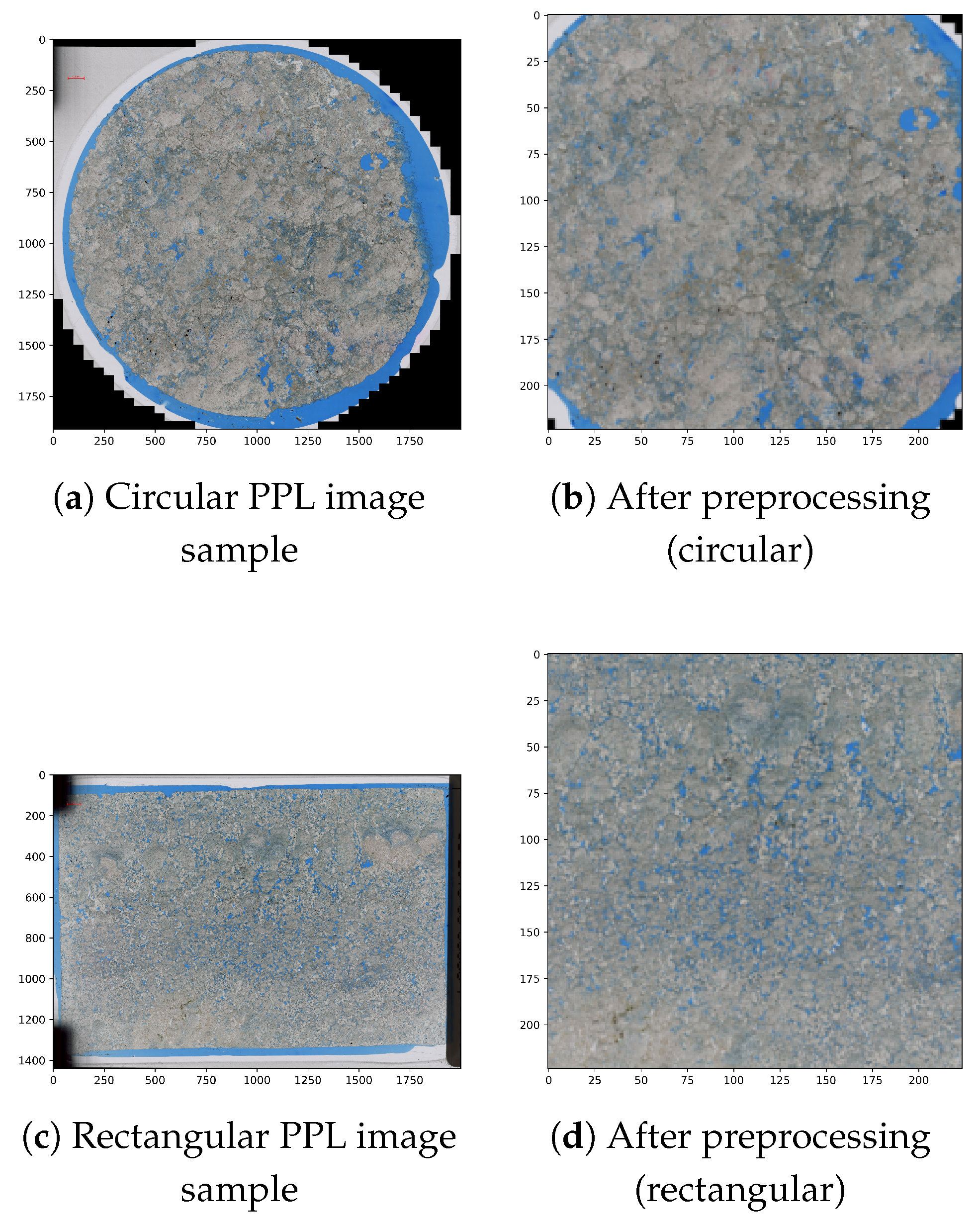
Figure 2.
Anomaly detection pipeline combining self-supervised learning and evaluation by a specialist.
Figure 2.
Anomaly detection pipeline combining self-supervised learning and evaluation by a specialist.
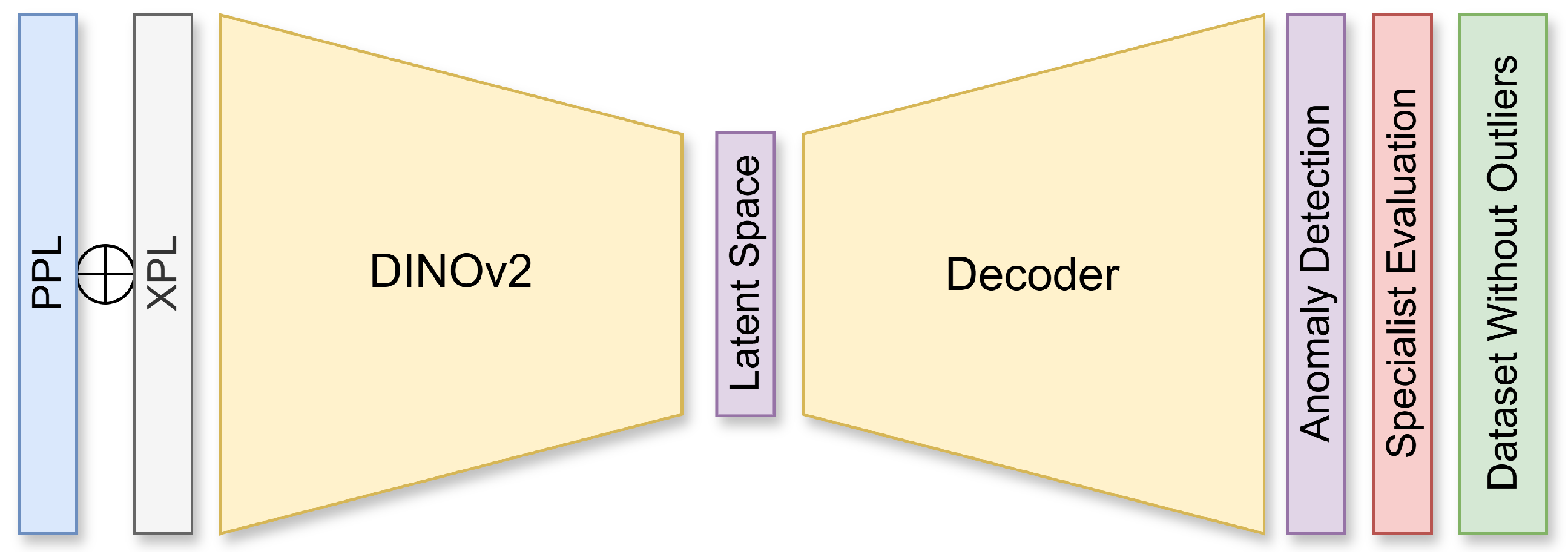
Figure 3.
Porosity vs. permeability for the analyzed samples. A log scale is used for permeability to highlight low-to-high transitions. Spearman’s rank correlation indicates a positive relationship.
Figure 3.
Porosity vs. permeability for the analyzed samples. A log scale is used for permeability to highlight low-to-high transitions. Spearman’s rank correlation indicates a positive relationship.
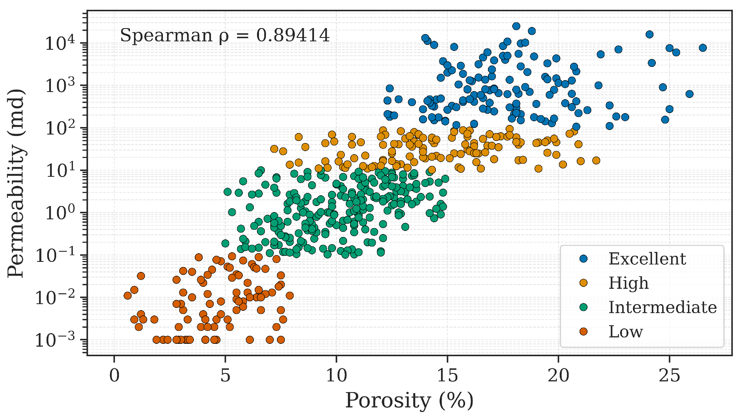
Figure 4.
Five-fold cross-validation strategy. In each iteration, a different fold is used for validation, and the rest for training.
Figure 4.
Five-fold cross-validation strategy. In each iteration, a different fold is used for validation, and the rest for training.
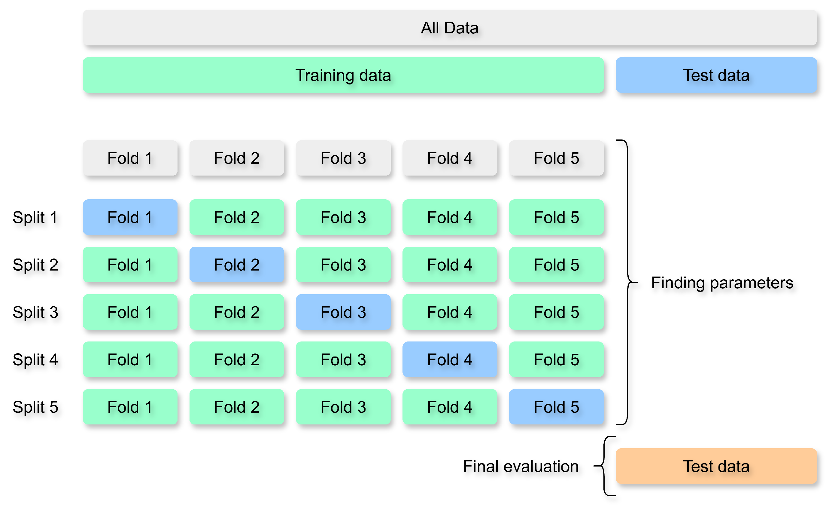
Figure 5.
Focal Loss behavior for different values of , adapted from [38]. As increases, the contribution of easy examples is further reduced.
Figure 5.
Focal Loss behavior for different values of , adapted from [38]. As increases, the contribution of easy examples is further reduced.
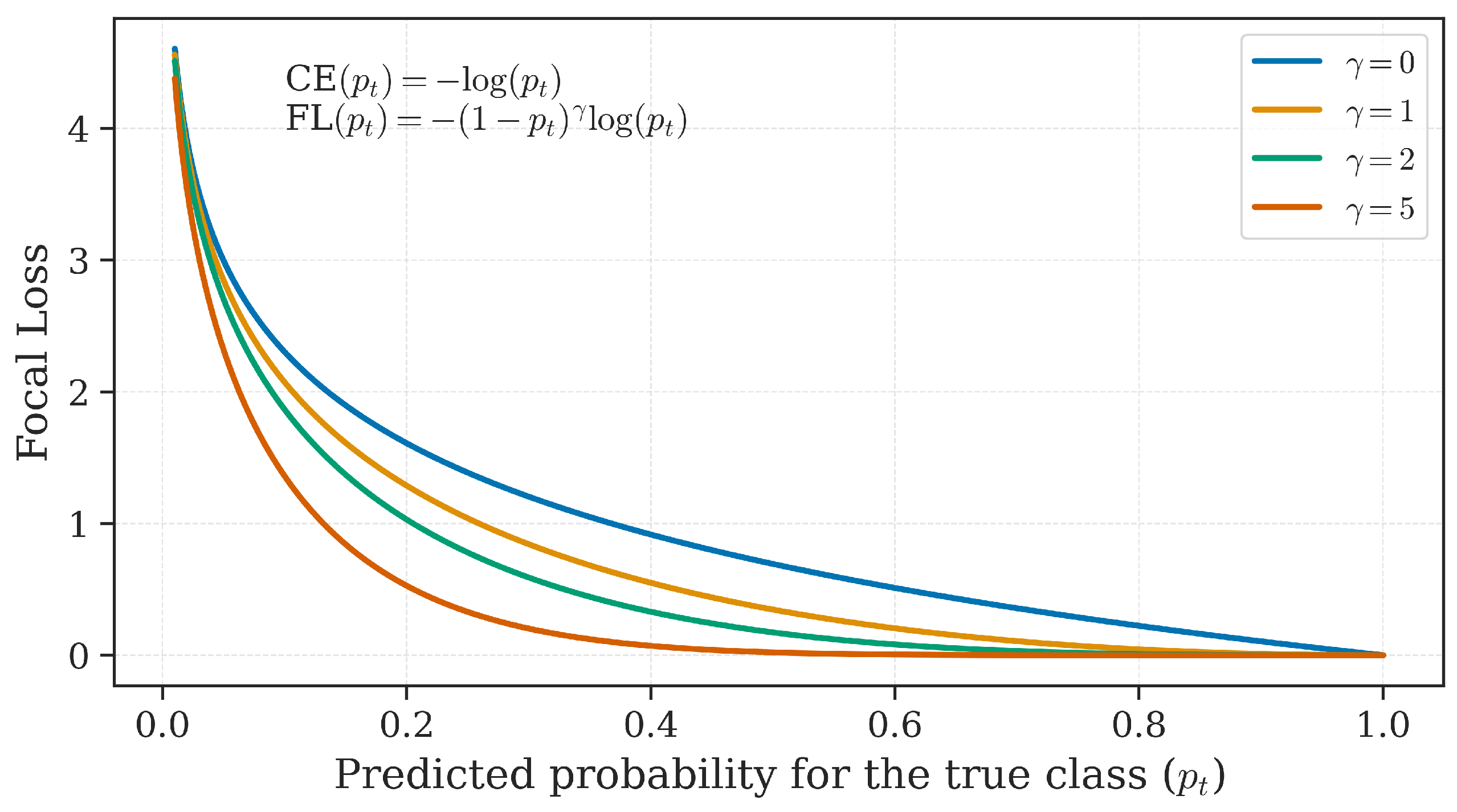
Figure 6.
Fine-tuning pipeline: PPL and XPL images are preprocessed and fused into a 6-channel input, then passed to a pre-trained backbone with a new classification head.
Figure 6.
Fine-tuning pipeline: PPL and XPL images are preprocessed and fused into a 6-channel input, then passed to a pre-trained backbone with a new classification head.
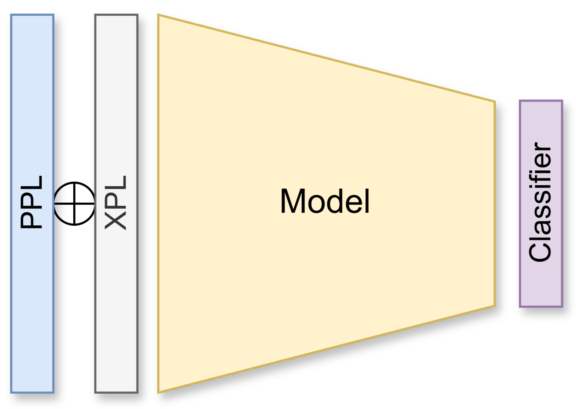
Figure 7.
Training and validation behavior of the ViT-B/8 model during training. Curves represent the average across five-folds, and shaded areas indicate standard deviation.
Figure 7.
Training and validation behavior of the ViT-B/8 model during training. Curves represent the average across five-folds, and shaded areas indicate standard deviation.
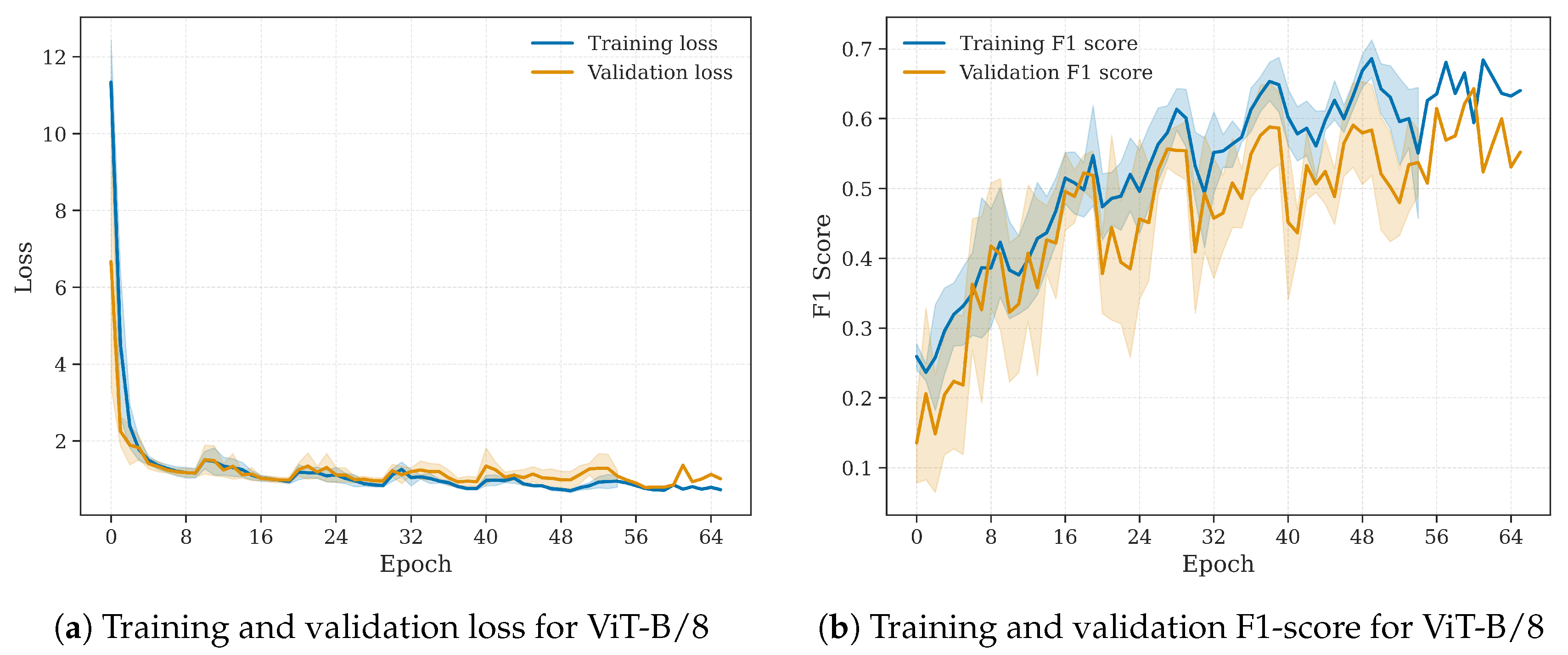
Figure 8.
Confusion matrices showing classification performance for each model: (a) ResNet, (b) DenseNet, (c) Vision Transformer (ViT), and (d) Swin Transformer. Color intensity represents the number of samples per class.
Figure 8.
Confusion matrices showing classification performance for each model: (a) ResNet, (b) DenseNet, (c) Vision Transformer (ViT), and (d) Swin Transformer. Color intensity represents the number of samples per class.
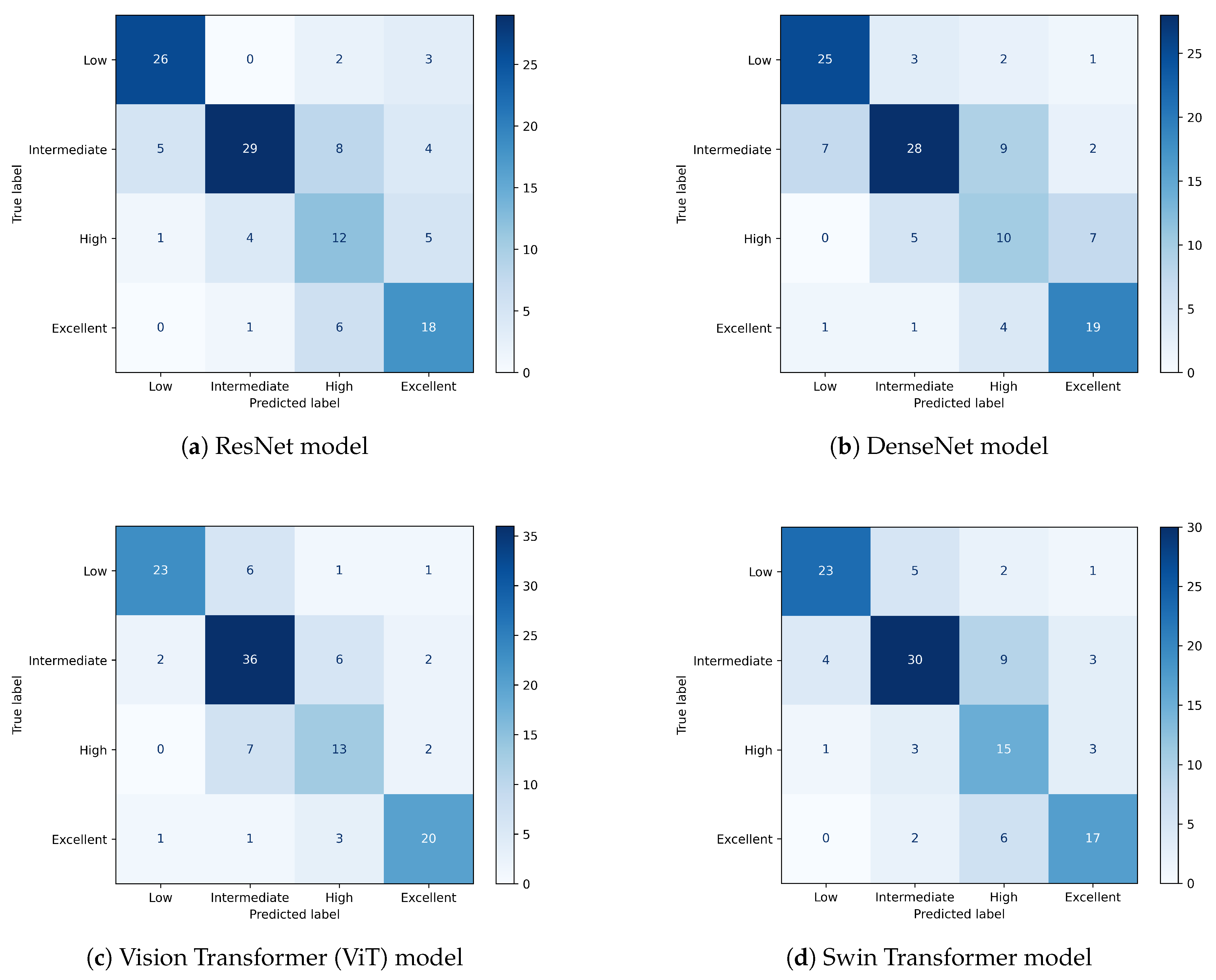
Figure 9.
Porosity–permeability cross-plot for the test set using the ViT-B/8 ensemble model. Each sample is colored by its true class. Misclassified samples are marked with a cross symbol and adopt the color of the predicted class. Permeability is shown on a logarithmic scale, and dashed lines represent the class boundaries.
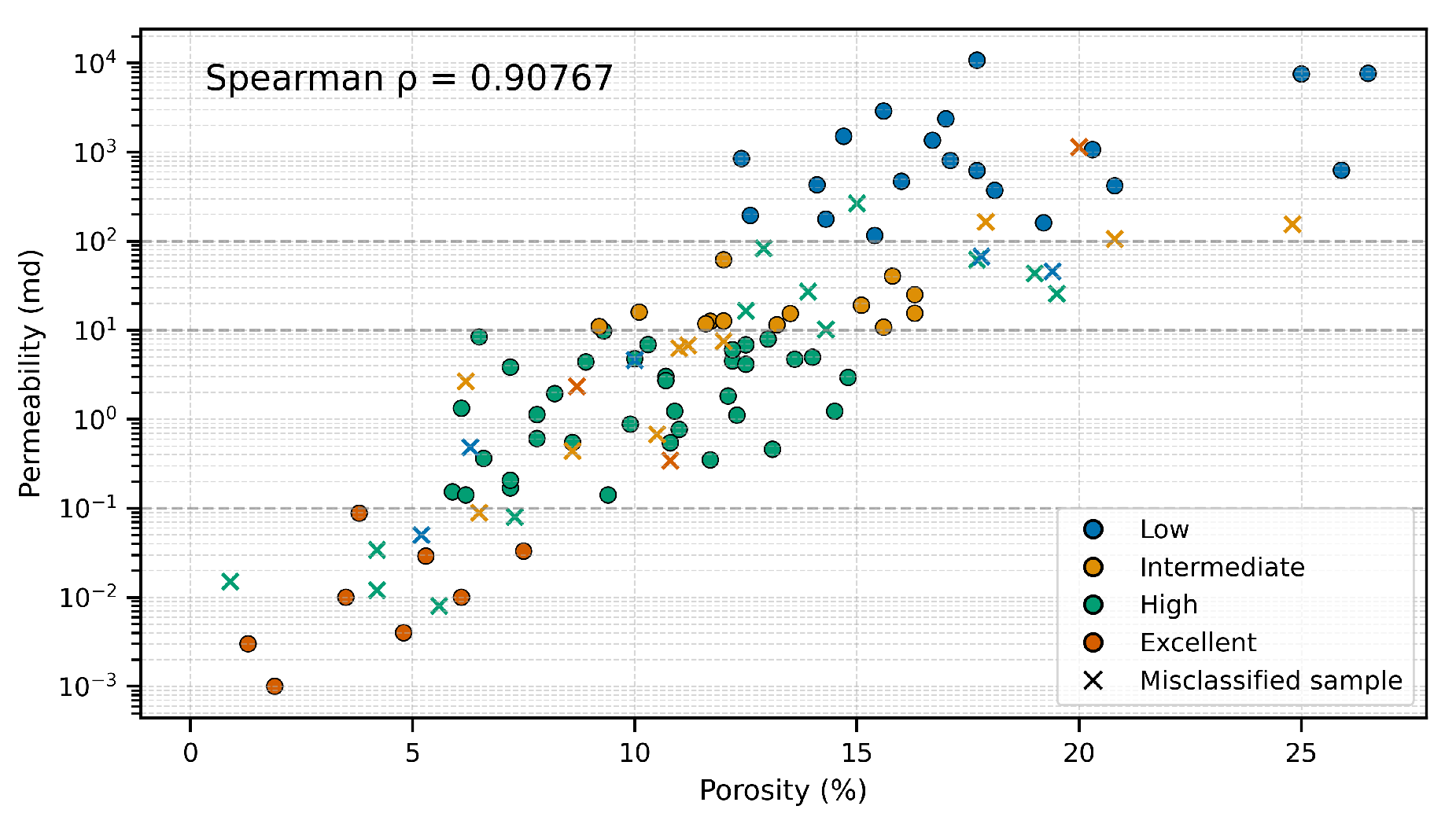

Table 1.
Permeability intervals and corresponding class definitions.
| Permeability (md) | Class | Samples | Percentage (%) |
|---|---|---|---|
| 0 – 0.1 | Low | 153 | 23.72 |
| 0.1 – 10 | Intermediate | 232 | 35.97 |
| 10 – 100 | High | 123 | 19.07 |
| ≥100 | Excellent | 137 | 21.24 |
| Total | — | 645 | 100.00 |
Table 2.
Best hyperparameters selected by Optuna for each model, including learning rate and RandAugment settings.
Table 2.
Best hyperparameters selected by Optuna for each model, including learning rate and RandAugment settings.
| Model | Learning Rate | Number of Transformations | Magnitude |
|---|---|---|---|
| ResNet-50 | 0.00586 | 3 | 12 |
| DenseNet-201 | 0.00781 | 3 | 9 |
| ViT-B/8 | 0.00373 | 2 | 6 |
| Swin-L | 0.00628 | 2 | 14 |
Table 3.
Average macro F1-score of each model over five independent test evaluations.
| Model | Average Macro F1-Score |
|---|---|
| ResNet-50 | 0.64074 ± 0.02296 |
| DenseNet-201 | 0.57408 ± 0.06085 |
| ViT-B/8 | 0.66084 ± 0.05254 |
| Swin-L | 0.64053 ± 0.02473 |
Table 4.
Classification results for each class and model. Precision, recall, and F1-score are reported per class, along with overall accuracy and macro F1-score.
Table 4.
Classification results for each class and model. Precision, recall, and F1-score are reported per class, along with overall accuracy and macro F1-score.
| Class | ResNet-50 | DenseNet-201 | ViT-B/8 | Swin-L | Support1 | ||||||||
|---|---|---|---|---|---|---|---|---|---|---|---|---|---|
| Prec. | Recall | F1 | Prec. | Recall | F1 | Prec. | Recall | F1 | Prec. | Recall | F1 | ||
| Low | 0.81 | 0.84 | 0.83 | 0.76 | 0.81 | 0.78 | 0.88 | 0.74 | 0.81 | 0.82 | 0.74 | 0.78 | 31 |
| Intermediate | 0.85 | 0.63 | 0.73 | 0.76 | 0.61 | 0.67 | 0.72 | 0.78 | 0.75 | 0.75 | 0.65 | 0.70 | 46 |
| High | 0.43 | 0.55 | 0.48 | 0.40 | 0.45 | 0.43 | 0.57 | 0.59 | 0.58 | 0.47 | 0.68 | 0.56 | 22 |
| Excellent | 0.60 | 0.72 | 0.65 | 0.66 | 0.76 | 0.70 | 0.80 | 0.80 | 0.80 | 0.71 | 0.68 | 0.69 | 25 |
| Accuracy | 0.69 | 0.66 | 0.74 | 0.69 | |||||||||
| Macro F1 | 0.67 | 0.65 | 0.73 | 0.68 | |||||||||
1 The support column indicates the number of test samples available for each class.
Disclaimer/Publisher’s Note: The statements, opinions and data contained in all publications are solely those of the individual author(s) and contributor(s) and not of MDPI and/or the editor(s). MDPI and/or the editor(s) disclaim responsibility for any injury to people or property resulting from any ideas, methods, instructions or products referred to in the content. |
© 2025 by the authors. Licensee MDPI, Basel, Switzerland. This article is an open access article distributed under the terms and conditions of the Creative Commons Attribution (CC BY) license (http://creativecommons.org/licenses/by/4.0/).
Copyright: This open access article is published under a Creative Commons CC BY 4.0 license, which permit the free download, distribution, and reuse, provided that the author and preprint are cited in any reuse.


