
Submitted:
20 July 2025
Posted:
22 July 2025
You are already at the latest version
Abstract
The Giesekus model has proven to be one of the most successful constitutive rheological models. Although Giesekus introduced the anisotropicity parameter as a constant, recent evidence suggests that it should not be. We herein elaborate on the implications of having a variable anisotropicity coefficient which, to our knowledge, has not been considered before. We find that the modification leads to important differences in the predictions of the second normal stress coefficient in simple shear flow, of which the most significant is the shift of the linear viscoelastic envelope of the second normal stress coefficient to higher values in the case of startup simple shear flow, which is more in line with literature experimental data.
Keywords:
rheological model
; polymer melts
; Giesekus model
; mobility tensor
; friction tensor
; Curtiss-Bird model
; link tension coefficient
1. Introduction
The use of plastic in almost every aspect of our everyday lives positions the plastic industry as one of the most important industries. Thus, the optimization of processes producing polymeric materials is of the utmost importance to avoid process instabilities [1,2]. Such a task necessitates the execution of numerical simulations that at heart employ an accurate and reliable constitutive rheological model that is based on molecular principles [2].The Giesekus model is widely regarded as one of the most successful constitutive equations for polymer solutions and melts, as it can predict a nonzero second normal stress difference, stress overshoot at the onset of simple shear flow, and finite extensional viscosity [3,4,5,6,7]. It introduces the notion that in sufficiently concentrated solutions and polymer melts, the frictional properties should be anisotropic [8,9], controlled by the magnitude of the anisotropicity or Giesekus parameter, α. By using the phase-space theory for concentrated polymer solutions and polymer melts of Curtiss and Bird [10,11,12], Giesekus [13] showed that his anisotropicity parameter can be related to the so-called link tension coefficient ε via . Stephanou et al. [14,15] provided the theoretical basis indicating that the link tension coefficient should not be considered a constant but should depend on the nematic order parameter. The revised framework predicts a vanishing ε at equilibrium, which remedies the erroneous predictions of the Curtiss-Bird model when considering a constant ε, namely the approach of the transient shear viscosity as t→0 to a constant value and the spurious sign changes of the transient second normal stress coefficient in startup simple shear flow.
Given the modification proposed by Stephanou et al. [14,15], in this work, we herein revisit the original Giesekus model by considering a non-constant anisotropicity parameter following the relationship between α and ε, and the relation between the former and the nematic order parameter as proposed by Stephanou et al. [14,15]. As such, at equilibrium, the anisotropicity parameter is equal to ½. We elaborate on the implications on the modified Giesekus predictions when considering a variable anisotropicity parameter and discuss whether its predictions are more in line with rheological experimental data. In Sec. 2, we provide the original and modified Giesekus constitutive model, and proceed to Sec. 3, where we present a comparison between their predictions. We conclude in Sec. 4 where the most important outcomes of our work are summarized and where we provide our future plans.
2. Constitutive Model
We consider an isothermal and incompressible flow. The Giesekus model in this case reads as follows [16]:
where c is the dimensionless conformation tensor and we have defined the upper-convected time derivative:
For the dimensionless mobility tensor, we consider the linear expression considered by Giesekus [13,16], namely,
where is the anisotropicity or Giesekus parameter. Also, the stress tensor is given as,
In this work, which we believe to be the first such work,we consider the Giesekus parameter to be given explicitly by the expression relating it to the link tension coefficient,
where is a constant coefficient and
is the nematic order parameter [17] which depends on the anisotropic orientation tensor defined as [14,15]
where I is the unit tensor and u the unit end-to-end vector of polymer chains. Note that the link tension coefficient is not constant: it vanishes at equilibrium, it increases with time in startup flows, and its steady-state value increases with the imposed flow rate [14]. By considering , then
As a final note, since the order parameter asymptotes at large shear rate to unity, the Giesekus parameter approaches the value ; since thermodynamic admissibility dictates that the Giesekus parameter should be [16,18,19,20] we need to bound . Finally, note that when α=0, the Giesekus model simplifies to the Upper-Convected Maxwell (UCM) one.
Asymptotic Behavior of the Model for Steady-State and Transient Shear Flow
We then analyze the asymptotic behavior of the two versions of the Giesekus model in the case of a steady and startup simple shear flow (SSF), described by the kinematics where y denotes the Cartesian coordinate and the shear rate. We present the following material functions: the shear viscosity and the first and second normal stress coefficients, and , respectively. The asymptotic behaviour is the same as the original Giesekus model, minus the fact that in the modified model that at equilibrium α=1/2 irrespective of the choice of . Thus, for the original model
whereas for the modified model,
We thus obtain the zero-shear-rate material functions: for the original model
and for the modified model,
Upon inception of the simple shear flow, we follow the methodology of Stephanou et al. [20] to obtain the explicit solutions for the time-dependent viscometric functions in the linear viscoelastic (LVE) limit. The results are the same as those of the original Giesekus model,
except for the fact that the LVE envelope of the second normal stress coefficient for the modified version differs,
3. Results and Discussion
3.1. Model Predictions in Steady-State Shear Flow
Figure 1 illustrates the variations in the conformation tensor components as functions of the dimensionless shear rate (Wi) in the case of steady-state SSF when the original Giesekus model is compared with the modified model at two different values of or (0.1 and 0.7). The behavior of as a function of Wi is the same for both models when small values of or (=0.1) are used. Similarly, as expected for small Wi (Wi < 0.1), remains close to its equilibrium value of unity in both models and then increases as Wi increases. This is expected since in the linear regime the mobility tensor is equal to the unit tensor. However, when or is raised to 0.7, we note that the two models provide different predictions in the intermediate range (0.1 < Wi < 100) with the modified model consistently predicting lower values than the original model. However, at large shear rates, the two models agree again, since in this case and due to Eq. (3a) . A similar behavior is noted also for [Figure 1(b)] and [Figure 1(c)]: in both cases, the predictions from the two models are the same at small and large shear rates, whereas the prediction of the modified model is below the original model’s one in the intermediate range. The scaling at large shear rates is the same for both models: increases as , reaches an asymptotic value, and decreases as . Then, Figure 2 shows the variations of the material viscometric functions as a function of Wi for both the modified and original models. For the shear viscosity and the first normal stress coefficient, we note a similar behavior as for the conformation tensor: the two models provide similar predictions for and for small and large shear rates, but the prediction of the modified model is below that of the original model predictions in the intermediate range. On the contrary, the behavior in the scaled second normal stress coefficient, , is quite different [Figure 2(c)]: the two models provide a similar prediction for a small value of or (= 0.1), with a similar zero-shear rate value (equal to 9/21 for the original model and ½ for the modified model) as dictated by Eqs. (5), and the scaling at large shear rates is , , and (Table 7.3-5 of Bird et al. [6]); however, they differ significantly at low and intermediate shear rates at larger values of or (= 0.7): the original Giesekus model predicts to be equal to 1/9, whereas the modified version always predicts it to be equal to ½. This also has implications to the startup behavior as will be described below.
3.2. Model Predictions in Steady-State Uniaxial Elongational Flow
In the case of uniaxial elongational flow (UEF), described by the kinematics , where is the elongation rate (x is the flow direction, y is the velocity gradient direction, and z is the neutral direction), the material function to be analyzed is the elongational viscosity, . A simple analytical solution can easily be obtained:
so that
The result Eq. (7b) is well-known (see Table 7.3-5 with λ2=0 in Bird et al. [6]). In the case of the original Giesekus model, the Giesekus parameter is a constant, whereas in the modified version it is given from Eq. (3a). In both models, the elongation viscosity reaches the asymptote as we may easily note from Eq. (7b) (also see Eq. (7B.8-4) of Bird et al. [6]).
Figure 3 shows the conformation tensor elements , , and the dimensionless elongation viscosity () versus Wi. In Figure 3(a), starts from its equilibrium value of unity at low Wi for both models, and then increases with Wi, with higher values as or increases to 0.7. Similarly, in Figure 3(b), also starts from its equilibrium value of unity at low Wi for both models, but then decreases as the shear rate increases, exhibiting higher values as or increases. The elongation viscosity starts from the value of 3, as per Trouton’s law, and increases as the elongation rate increases, exhibiting smaller values as or increases [Figure 3(c)]. When = 0.1, both models provide similar predictions for both and , whereas the prediction of the modified model is below the prediction of the original model for ; on the contrary, it seems that the prediction for is the same for both models, even with a larger value of or . The predictions for are noted to be the same for both models at large values of or whereas at smaller values, the modified version is below the original Giesekus model’s prediction in the intermediate range of elongation rates. The scaling at large shear rates is the same for both models, namely and , whereas, as mentioned above, the elongation viscosity always reaches the asymptote .
3.3. Model Predictions in Start-Up Shear Flow
Figure 4 and Figure 5 show the dimensionless material functions , , and for startup SSF as a function of dimensionless time for = 0.1 and = 0.7, respectively, at Wi = 1, 10, and 100. In Figures 4(a) and 4(b), the predictions of and for both models exhibit similar overall trends for all Wi: they increase at early times following the LVE envelope, Eqs. (6), reach an overshoot and then decrease, before reaching their steady state value. Also, both models' predictions the shear viscosity present an undershoot after the overshoot, which is more easily noticeable at Wi=100. This oscillatory behavior for the original Giesekus model was first noted by Giesekus [8]. Such undershoots, first provided by the experimental work of Costanzo et al. [21], has been associated with the tumbling of polymer chains in simple shear [22,23]. When or is small (=0.1), the predictions of the original and modified Giesekus models are identical, as seen in Figure 4, whereas at a larger value (=0.7), there are clear differences between the original and modified models (Figure 5). In particular, the predictions of the modified Giesekus model for and are noted to be below the original Giesekus model predictions at large times for intermediate shear rates (Wi=1 and 10), whereas the predictions are similar at larger shear rates irrespective of time. On the other hand, the predictions of the two models for are noted to be completely different even in the LVE regime, as indicated by the different expressions for the LVE envelope [see Eqs. (6)]. The modified model is seen to shift upwards following Eq. (6b) and is noted to predict a larger value than the original model at small shear rates (Wi=1). However, at larger shear rates (Wi=10 and 100), both models exhibit the same steady-state value. This behavior is more in line with experimental data [14]; as seen in Figure 8(b) of Stephanou et al. [20], the LVE envelope predicted by the original Giesekus model (note that the LVE envelope provided there is not exactly the same as the original Giesekus model provided here; however, due to the very small value of the slip parameter considered in their work, ξ=0.03, their LVE envelope should not differ substantially from the original Giesekus model one) is below the LVE envelope suggested by the experimental data. Thus, the use of a variable Giesekus parameter, as done in the modified model, would certainly improve the comparison against said experimental data.
4. Conclusions
The Giesekus model has accumulated since its introduction in the early 1980s increased attention due to its simplicity and its capacity to conform to various experimental attributes [3]. Giesekus [13], to validate his postulate, showed that his expression for the mobility tensor can be obtained through a linearization of the mobility tensor proposed in phase-space theory for concentrated polymer solutions and polymer melts of Curtiss and Bird [10,11,12], which allowed him to relate his anisotropicity parameter to the link tension coefficient of Curtiss-Bird. However, recent evidence by Stephanou et al. [14,15] unambiguously shows that the link tension coefficient should not be considered a constant but should depend on strain rate and time via the nematic order parameter. Since the implications of using a variable anisotropicity parameter have not been presented before, in this work, we provide the predictions of a modified Giesekus parameter where the Giesekus parameter is no longer constant. Under steady-state simple shear flow, we note that the two models exhibit the same behaviour when or is small, and at any value of or at small and large shear rates. A similar behavior is noted for the transient shear viscosity and the transient first normal stress coefficient in start-up simple shear flow; however the predictions are noted to be very different in the case of the transient second normal stress coefficient in start-up simple shear flow where the LVE envelope is noted to shift to larger values, which is more in line with experimental data [14,20]. We thus expect that the use of a variable Giesekus parameter will improve the predictive capacity of constitutive models that employ the Giesekus parameter to more accurately predict the rheological behaviour of polymeric systems. We aim to undertake such an improvement of the Stephanou et al. [20] in the future.
Author Contributions
Fatemeh Karami: Software (equal); Validation (equal); Formal analysis (equal); Investigation (equal); Data curation (equal); Writing – original draft (equal); Writing – review & editing (supporting); Visualization (equal). Pavlos S. Stephanou: Conceptualization; Methodology; Software (equal); Validation (equal); Formal analysis (equal); Investigation (equal); Data curation (equal); Writing – original draft (equal); Writing – review & editing (lead). Supervision; Visualization (equal); Project administration.
Funding
This research received no funding
Data Availability Statement
The data that support the findings of this study are available within the article.
Conflicts of Interest
The authors declare no conflict of interest.
References
- Graham, M.D. The Sharkskin Instability of Polymer Melt Flows. Chaos 1999, 9, 154–163. [CrossRef]
- Tadmor, Z.; Gogos, C.G. Principles of Polymer Processing; 2nd Editio.; Wiley-Interscience: Hoboken, NJ, USA, 2006; ISBN 978-0-471-38770-1.
- Germann, N. Preface to Special Topic: One Hundred Years of Giesekus. Phys. Fluids 2024, 36, 050401.
- Larson, R.G. The Structure and Rheology of Complex Fluids; Oxford University Press: New York, United States, 1999; ISBN 9780195121971.
- Larson, R.G. Constitutive Equations for Polymer Melts and Solutions; 1st ed.; Butterworth-Heinemann, 1988; ISBN 978-0-409-90119-1.
- Bird, R.B.; Armstrong, R.C.; Hassager, O. Dynamics of Polymeric Liquids. Volume 1. Fluid Mechanics.; 2nd Editio.; Wiley-Interscience, 1987; ISBN 047107375X.
- Tanner, R.I. Engineering Rheology; 2nd ed.; Oxford Engineering Science Series, 2002; ISBN 9780198564737.
- Giesekus, H. Stressing Behaviour in Simple Shear Flow as Predicted by a New Constitutive Model for Polymer Fluids. J. Nonnewton. Fluid Mech. 1983, 12, 367–374. [CrossRef]
- Giesekus, H. On Configuration-Dependent Generalized Oldroyd Derivatives. J. Nonnewton. Fluid Mech. 1984, 14, 47–65. [CrossRef]
- Bird, R.B.; Curtiss, F.C.; Amstrong, C.R.; Ole, H. Dynamics of Polymeric Liquids, Second Edition Volume 2: Kinetic Theory; Wiley-Interscience, 1987; ISBN 978-0-471-80244-0.
- Curtiss, C.F.; Byron Bird, R. A Kinetic Theory for Polymer Melts. I. The Equation for the Single-Link Orientational Distribution Function. J. Chem. Phys. 1980, 74, 2016–2025. [CrossRef]
- Curtiss, C.F.; Byron Bird, R. A Kinetic Theory for Polymer Melts. II. The Stress Tensor and the Rheological Equation of State. J. Chem. Phys. 1980, 74, 2026–2033. [CrossRef]
- Giesekus, H. A Simple Constitutive Equation for Polymer Fluids Based on the Concept of Deformation-Dependent Tensorial Mobility. J. Nonnewton. Fluid Mech. 1982, 11, 69–109. [CrossRef]
- Stephanou, P.S.; Schweizer, T.; Kröger, M. Communication: Appearance of Undershoots in Start-up Shear: Experimental Findings Captured by Tumbling-Snake Dynamics. J. Chem. Phys. 2017, 146, 161101. [CrossRef]
- Stephanou, P.S.; Kröger, M. Non-Constant Link Tension Coefficient in the Tumbling-Snake Model Subjected to Simple Shear. J. Chem. Phys. 2017, 147, 174903. [CrossRef]
- Stephanou, P.S.; Baig, C.; Mavrantzas, V.G. A Generalized Differential Constitutive Equation for Polymer Melts Based on Principles of Nonequilibrium Thermodynamics. J. Rheol. 2009, 53, 309–337. [CrossRef]
- Kröger, M. Models for Polymeric AndAnisotropic Liquids; Springer-Verlag: Berlin Heidelberg, 2005; ISBN 978-3-540-26210-7.
- Beris, A.N.; Edwards, B.J. Thermodynamics of Flowing Systems: With Internal Microstructure; Oxford University Press: New York, 1994; ISBN 019507694X.
- Nikiforidis, V.-M.; Tsalikis, D.G.; Stephanou, P.S. On The Use of a Non-Constant Non-Affine or Slip Parameter in Polymer Rheology Constitutive Modeling. Dynamics 2022, 2, 380–398. [CrossRef]
- Stephanou, P.S.; Tsimouri, I.C.; Mavrantzas, V.G. Simple, Accurate and User-Friendly Differential Constitutive Model for the Rheology of Entangled Polymer Melts and Solutions from Nonequilibrium Thermodynamics. Materials (Basel). 2020, 13, 2867. [CrossRef]
- Costanzo, S.; Huang, Q.; Ianniruberto, G.; Marrucci, G.; Hassager, O.; Vlassopoulos, D. Shear and Extensional Rheology of Polystyrene Melts and Solutions with the Same Number of Entanglements. Macromolecules 2016, 49, 3925–3935. [CrossRef]
- Kim, J.M.; Baig, C. Precise Analysis of Polymer Rotational Dynamics. Sci. Rep. 2016, 6, 19127. [CrossRef]
- Nafar Sefiddashti, M.H.; Edwards, B.J.; Khomami, B. Individual Chain Dynamics of a Polyethylene Melt Undergoing Steady Shear Flow. J. Rheol. 2015, 59, 119–153. [CrossRef]
Figure 1.
Model predictions for the conformation tensor components (a) , (b) , (c) , in steady SSF as a function of the dimensionless shear rate, and dependency on the parameter α for the original model, and for the modified model. The dotted lines depict the predictions of the UCM model (with ε=0).
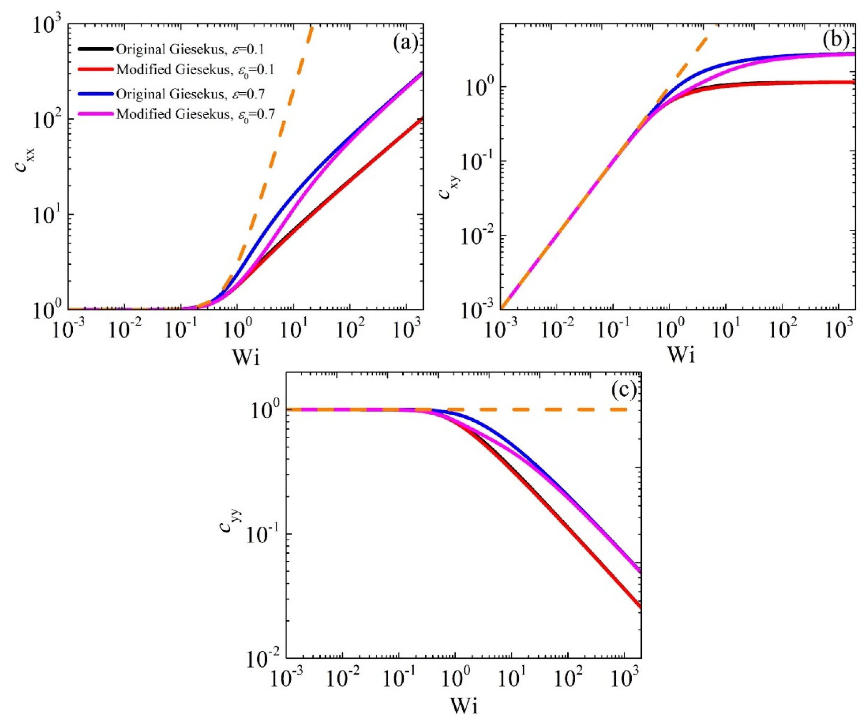
Figure 2.
Same as Figure 1 but for the viscometric functions.
Figure 2.
Same as Figure 1 but for the viscometric functions.
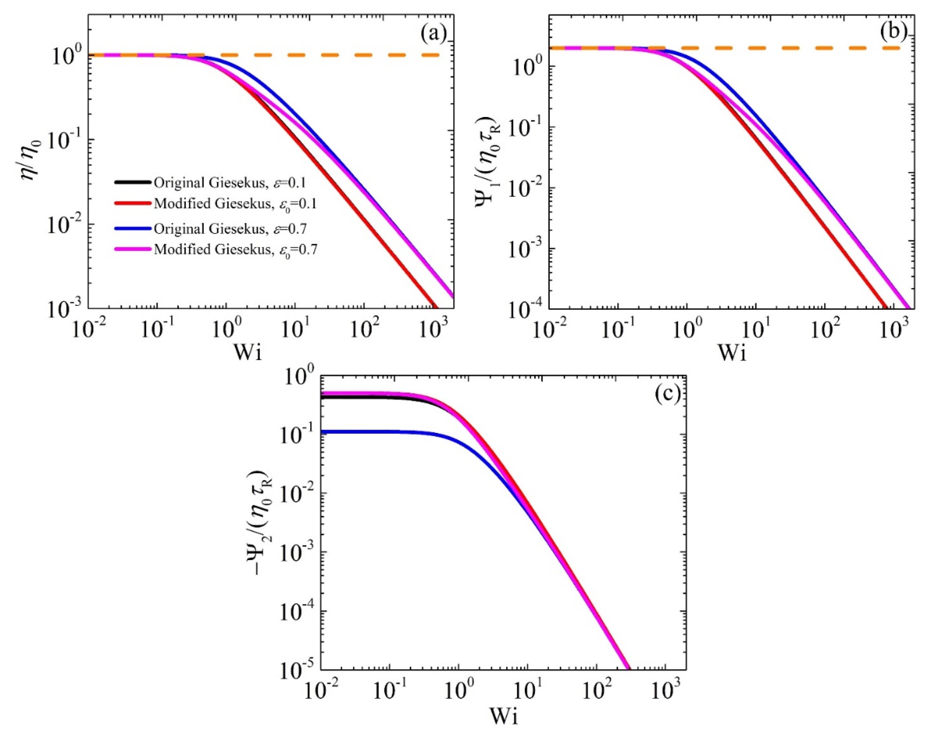
Figure 3.
Model predictions for the conformation tensor components (a) , and (b) , and (c) the scaled elongational viscosity in steady UEF as a function of the dimensionless elongation rate, and dependency on the parameter α for the original model and for the modified model. The dotted lines depict the predictions of the UCM model (with ε=0).
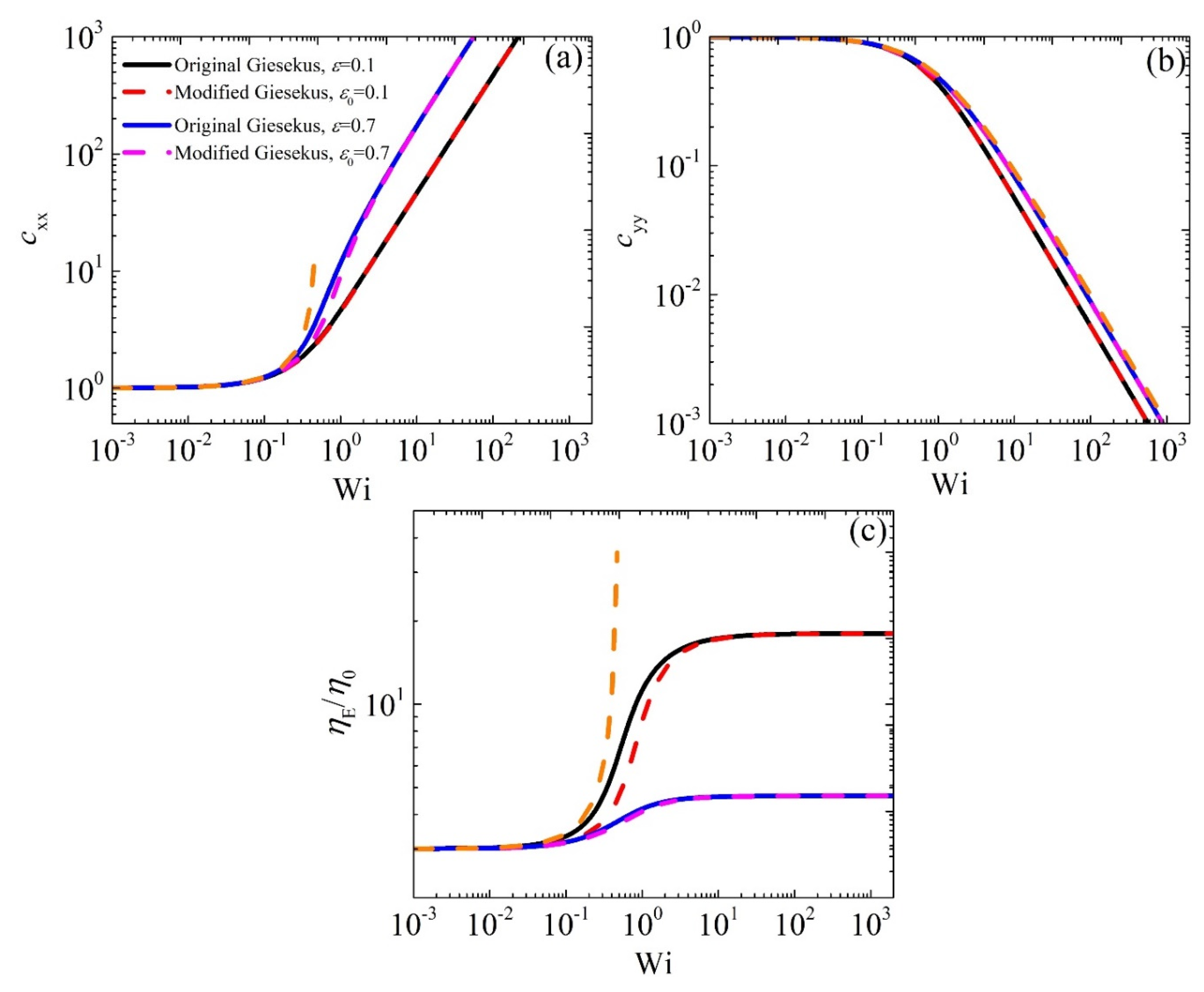
Figure 4.
Model predictions when for the growth of the (a) shear viscosity, (b) first normal stress coefficient, and (c) second normal stress coefficient, upon the inception of shear flow at different dimensionless shear rates as a function of dimensionless time. The dotted dark yellow lines in each panel and the dotted olive line in panel (c) depict the LVE envelope given by Eq. (6).
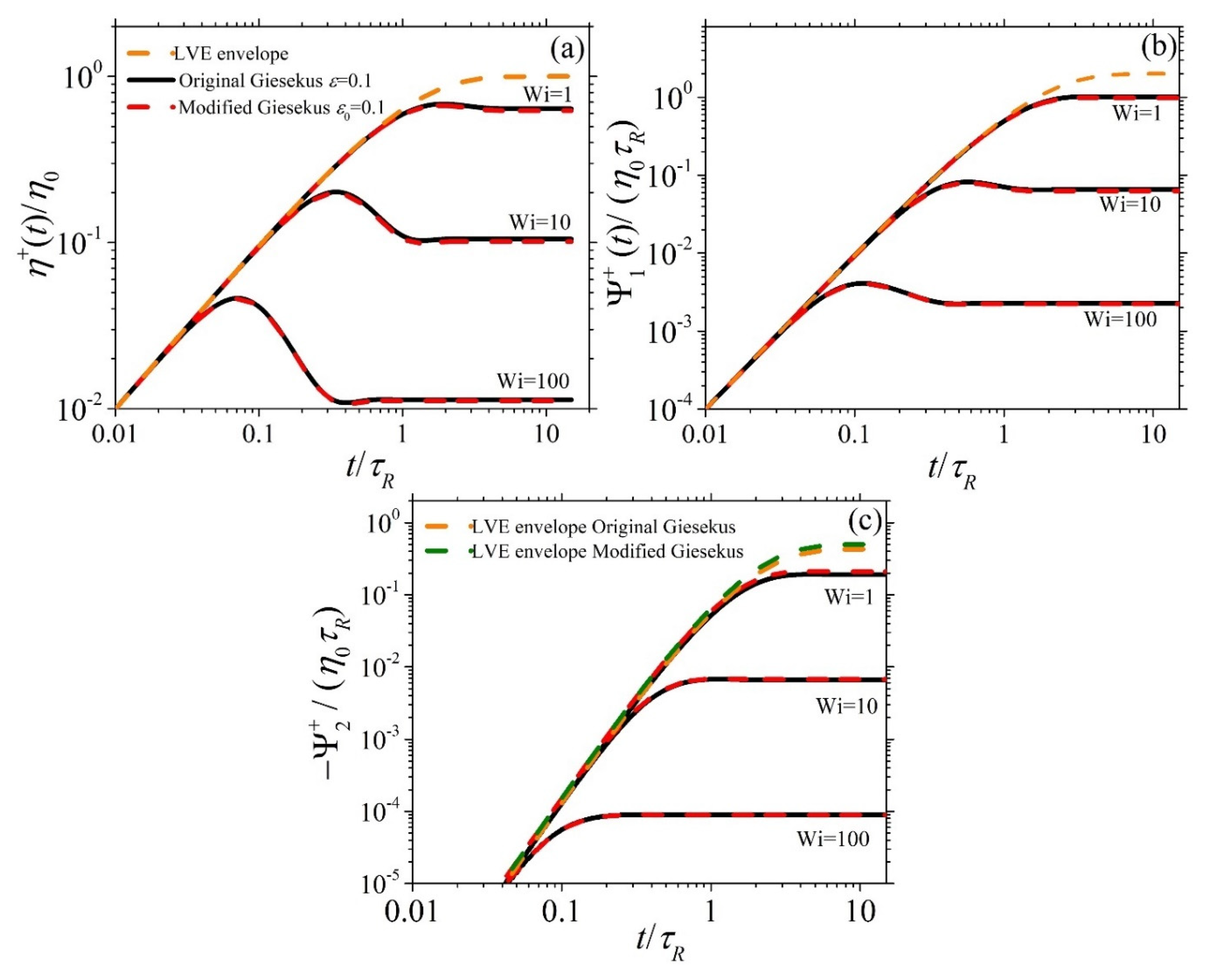
Figure 5.
Same as Figure 4 but for .
Figure 5.
Same as Figure 4 but for .

Disclaimer/Publisher’s Note: The statements, opinions and data contained in all publications are solely those of the individual author(s) and contributor(s) and not of MDPI and/or the editor(s). MDPI and/or the editor(s) disclaim responsibility for any injury to people or property resulting from any ideas, methods, instructions or products referred to in the content. |
© 2025 by the authors. Licensee MDPI, Basel, Switzerland. This article is an open access article distributed under the terms and conditions of the Creative Commons Attribution (CC BY) license (http://creativecommons.org/licenses/by/4.0/).
Copyright: This open access article is published under a Creative Commons CC BY 4.0 license, which permit the free download, distribution, and reuse, provided that the author and preprint are cited in any reuse.


