
Submitted:
19 July 2025
Posted:
22 July 2025
You are already at the latest version
Abstract
The aim of this article is to introduce the distributed-order hyperchaotic detuned (DOHD) laser model. Its dissipative dynamics, invariance, fixed points (FPs) and their stability are investigated. Numerical solutions of the DOHD laser model are computed using the modified Predictor-Corrector approach. Its viscoelasticity is described by the so-called DO derivative, allowing for the study of different technical systems and materials, and the model is found to have a whole circle of FPs as a hyperchaotic attractor. We discuss the coexistence of more attractors under various initial conditions and the same sets of parameters for our model (multistability). We also introduce the notion of dual combination synchronization (DCS), using four integer-order drive models and two DO response models. A theorem is stated and proved to obtain an analytical control function that ensures DCS for our models. Numerical simulations are presented to support these analytical results. Regarding the use of the well--known Caputo derivative, the results are very similar to those of DO, except when the Caputo order, $0< \sigma\gteq1$, is very close to $1$, where the dynamics shows a "spiralling behavior" towards a fixed point. In all other cases, both Caputo and DO exhibit a very similar behavior.
Keywords:
fractional derivatives
; distributed derivatives
; hyperchaotic
; detuned laser
; multistability
; synchronization
1. Introduction
The distributed-order (DO) fractional calculus was discussed for the first time in 1969 in [1]. It was argued then that the DO derivative is a generalization of fractional and integer-order derivatives. Caputo and others, in [2,3,4,5,6,7] developed what they called the DO calculus. DO differential equations have several uses in the fields of secure communication, image encryption, physics, and circuit implementation [8,9,10,11]. Aboelenen [12] proposed a local discontinuous Galerkin finite element approach for DO time, Riesz space-fractional convection-diffusion, and Schrödinger-type problems. In [13], chaos synchronization of the DO Lorenz model using chaotic masking are presented. Secure communications using DO hyperchaotic masking for a text that consists of symbols, spaces, numbers and alphabets are examined in [8]. Abed-Elhameed et. al [11] introduced a scheme for image encryption based on adaptive synchronization.
The authors of [14] proposed the complex detuned lasers model as follows:
where, , , , , the positive real parameters are a, b, c, and d, the complex conjugate variable is denoted by and the time derivatives are represented by dots. The state variables w, v, and u in a ring laser system of two-level atoms are related to population inversion, polarization, and electric field amplitude, respectively, as illustrated in [15]. The dynamics and synchronization characteristics of complex detuned lasers (1.1) were investigated by Mahmoud et al. [16], and in this 5-dimensional model [16] only chaotic attractors were found to exist . A new version of (1.1) which represents a 6-dimensional hyperchaotic model was studied in [17], where . Using a novel image cryptosystem for high security, Li et al. [18] discussed the 7-dimensional fractional-order hyperchaotic detuned laser model.
The real form of (1) is written as:
where, and are real state variables.
Based on the model (1.2), the fractional-order detuned laser model can be written as:
where, stands for the Caputo fractional derivative [1], , and and d are the real parameters of model (3).
In this paper, we focus on what we call the distributed-order hyperchaotic detuned (DOHD) laser model, given as follows:
Extreme multistability and multistability phenomena have recently become very important in the study of chaotic models. Indeed, multistability frequently appears in nonlinear dynamical systems and denotes the presence of multiple attractors for the same set of model parameters [19]. Additionally, this phenomenon is often referred to as extreme multistability when an infinite number of attractors coexist for the same set of model parameters [20]. An enhanced two stable node-foci example of Chua’s circuit was investigated and the model’s multistability was examined in [21]. In [22], coexisting chaotic attractors, as well as periodic and point attractors were studied in a new 4D smooth chaotic model. Chen [23] discovered many kinds of coexisting behaviors, such as coexisting chaotic and periodic attractors, chaotic attractors and singular degenerate heteroclinic cycles, different kinds of periodic attractors, as well as periodic attractors and singular degenerate heteroclinic cycles. Moreover, the phenomenon of extreme multistability, with an infinite number of hidden attractors was investigated in a novel memristive hyperchaotic model in [24]. Mengxin et al. [25] also observed the phenomenon of extreme multistability in a complex simplified Lorenz model with integer-order derivatives. Finally, a logarithmic memcapacitor model was comprehensively investigated with coexisting attractors and multistable coexisting oscillations in [26].
The synchronization of hyperchaotic (or chaotic) models is an essential branch of nonlinear dynamics research. It has been thoroughly studied in a number of areas, such as circuit implementation [11], neural networks [27], color image encryption [9] and secure communications [8]. Many types of synchronization, including complete synchronization [7], projective synchronization [27], adaptive synchronization [11] and generalization of combination synchronization [9] were investigated for DO models. A scheme to examine the generalization of combination-combination synchronization among two fractional-order and two DO hyperchaotic models was introduced in [28].
In this article, we present the dynamics and numerical solutions of the DOHD laser model (1.4) for the first time. The coexistence of several attractors with the same parameter set but different initial conditions is investigated, while we also study the dual combination synchronization (DCS) for integer and DO hyperchaotic models. Other types of synchronization can also be studied, as particular cases of the suggested DCS phenomenon, as noted in literature. Here, using the tracking control technique [29], we present schemes for the DCS with four drive and two response integer and distributed-order models, respectively. To derive analytical formulas for control functions, we formulate and prove a new theorem. A particular case is provided to demonstrate how well the numerical and analytical results agree with each other. To this end, we applied here the modified Predictor-Corrector approach [7] to obtain our numerical results.
The format of this article is as follows: A preliminary introduction and an application of the Caputo fractional derivative to our model are given in Section 2 and Section 3 respectively. Next, the dynamical properties and Lyapunov exponents (LEs) of the proposed model (1.4) are calculated in Section 4. Section 5 contains the numerical simulations of the multistability phenomenon for a model with various coexisting attractors. A scheme to achieve the DCS using the tracking control technique is investigated in Section 6. Furthermore, a particular case is provided to demonstrate the validity of the generated analytical control functions. Our overall conclusions are described in the final section.
2. Application of the Caputo Fractional Derivative to the Model (1.3)
In this Section, we use the classical form of the Caputo derivative, as stated in eq. (1.3) of Section 3 and present results on their chaotic behavior in Figure 1 and Figure 2 (see below). The reader is advised to inspect these figures, in connection with their corresponding data, described in the subsection that follows, and compare them with the results of the DO derivative presented in later sections of the paper.
2.1. Numerical Solutions of the Fractional-Order Detuned Laser Model (1.3)
The numerical solutions of the fractional-order detuned laser model (1.3) are computed applying the Predictor-Corrector technique [30]. We calculated the LEs by a modified technique of the well–known Wolf algorithm [31] implemented using a MATLAB software program. This model has five LEs . The signs of these LEs give a useful characterization of the dynamics of this model’s solutions [32]. For the following cases, we determined the LEs for an observation time 1000, sampling size 0.001 and the initial conditions , where T denotes the transpose.
2.1.1. Solutions That Approach Fixed Points
For model (1.3), if we choose , we obtain the following values of the LEs as: , , , and . These imply that the solution of model (1.3) approaches a stable fixed point in the 5-dimensional space and indeed we find numerically that it does. The same holds true for .
2.1.2. Solutions That Approach a Chaotic Attractor
2.1.3. The Difference Between Caputo and DO Dynamics
We emphasize that the DO derivative studied here extends the property of the dynamics, beyond the Caputo derivative, by integrating over all . Thus, as we describe below, it leads not only to stable fixed points, but also to chaotic and hyperchaotic attractors.
3. Preliminaries
In this section, we provide definitions, lemmas and a theorem [1,7,33] for our analysis of the DO derivative, which constitute the fundamental ideas of the paper.
Definition 1.
[1] For any For the function , the Caputo fractional derivative is defined as follows:
Definition 2.
Theorem 3.1.
[7] Assume that a dynamical system with DO on several terms of our fractional-order model is given by:
where, and let represent the eigenvalues of , if
where, f contains the nonlinear terms of our model, J is constant matrix, so that , , I is the identity matrix and is the number of steps for . It follows that (3.3) has a zero solution that is asymptotically stable.
Lemma 3.1.
where and . Thus, is Mittag-Leffler stable, where is a FP for the DO model (3.3). If these assumptions hold globally on , then is globally Mittag-Leffler stable.
Lemma 3.2.
[6] Let is differentiable function, then
where, T denotes the transpose operation.
4. Analysis of the DOHD Laser Model (1.4)
In this section, we examine the dissipation, invariance, FPs, stability, and coexistence properties of a hyperchaotic attractor of the DOHD laser model (1.4).
4.1. Invariance and Dissipation
Under the transformation , the model (1.4) is symmetric, and is the axis of rotational symmetry. The divergence of (1.4) is as follows:
Consequently, we can conclude that our model (1.4) is dissipative when .
4.2. Fixed Points and Their Stability
First, the FPs of model (1.4) can be obtained as follows:
One solution of (1.4) is clearly , which is the trivial FP, while we also obtain a circle of nontrivial FPs as follows:
, , , , , ,
where, and . So, model (1.4) has the circle of FPs: .
For model (1.4), we analyze the stability of by applying Theorem 3.1. The first condition of Theorem 3.1 can be tested using the following steps:
where .
We test a particular case by examining the second requirement of Theorem 3.1, as the stability cannot be known in general. The form of trivial FPs is: . Taking and , we find
where, , , I is identity matrix and J is the matrix of the linear part of model (1.4). The equivalent characteristic polynomial is:
this indicates that each point on this circle is stable if , ; else, it is a circle of unstable FPs.
4.3. Numerical Solutions of the DOHD Laser Model (1.4)
Utilizing the improved predictor-corrector technique [7], the numerical solutions for the DOHD laser model (1.4) are established. Our technique for calculating the LEs involves modifying the Wolf algorithm [31]. Clearly, there are five LEs for this model, and its solutions to this model are characterized by the signs of LEs [9]. Selecting and the initial conditions , where the LEs of the model (1.4) are calculated, for an observation time 30000 and sampling size 0.001, to be: and , see Figure 3. This indicates, as shown in Figure 4, that this model has a hyperchaotic attractor.
5. Coexisting Attractors of DOHD Laser Model (1.4)
In this section, we discuss the coexistence of more than one attractors, under various initial conditions, for the same sets of parameters, a phenomenon known as multistability. Model (1.4) has many coexisting attractors for the various ranges of initial conditions.
5.1. Chaotic and Hyperchaotic Attractors
This subsection deals with the generating many coexisting multiple attractors of model (1.4) by various ranges of initial conditions and fixing the parameters and d. We calculated the LEs for model (1.4) with various ranges of initial conditions and the same sets of parameters for the following cases:
5.1.1. Fix , , , , and Vary
We determined the LEs for the initial condition of of model (1.4) as seen in Figure 5. This model has a hyperchaotic attractor for and and it has chaotic attractors for and .
For and the initial condition , the solutions of (1.4) converge to a hyperchaotic attractor . The corresponding LEs of this hyperchaotic attractors are
, , , and .
When and the initial condition , the solution of the model (1.4) goes to a chaotic attractor . Also, the related LEs of this chaotic attractor are
, , , and .
The phase space of and are seen in Figure 6.
5.1.2. Fix , , , , and Vary
By computing the LEs for model (1.4) for the initial condition of , e conclude that our model has a hyperchaotic attractor for and for it has a chaotic attractor.
5.1.3. Fix , , , , and Vary
For the initial condition of , model (1.4) has a hyperchaotic attractor for and for it has chaotic attractors.
5.1.4. Fix , , , , and Vary
As we did before, we concluded that for , model (1.4) has a hyperchaotic attractor for and it has chaotic attractors for .
5.1.5. Fix , , , , and Vary
Under the initial condition , our model (1.4) has a hyperchaotic attractor for and it has chaotic attractors for .
5.2. Solution That Approaches Fixed Points
In a similar way as we did above, we evaluated the LEs for the following case:
5.2.1. Fix , , , and Vary the Initial Conditions
The solution of model (1.4) approaches FPs for any values of initial conditions. For example, if we choose , , , and , we computed the LEs which are: , , , and . This means that our solution approaches FPs at these initial conditions as seen in Figure 7.
6. A Scheme for DCS Between Integer and Distributed-Order Hyperchaotic Models
The DCS of n-dimensional hyperchaotic integer-order and DO dynamical systems with four drive and two response models are introduced in this part. For the drive models, we need one pair of two integer-order hyperchaotic models, and for the response models, we need another pair of DO hyperchaotic models.
Let the drive models be:
and
where, the state vectors of drive models (6.1,6.2) are , , , and the four continuous vector functions , , , .
Models (6.1,6.2)) can be expressed as
and
where, , , and .
These are the equivalent of one pair of two response models:
where, , is the state vectors of the response models (6.5), and are continuous vector functions and , are two control functions of the response models (6.5).
Models (6.5) can be expressed in vector form as:
where, , and .
Definition 3.
Given that three non-zero constant diagonal matrices and S in exist, such that
then the drive models (6.3-6.4) are said to be in DCS with the response models (6.6), where the synchronization error is , while the matrix norm is .
Remark 6.1.
Equation (6.7) implies combination synchronization [17] if the response models are integer-order.
Remark 6.2.
Assume the following for the control function :
with the the compensation control described as:
The vector of the control function will be defined below.
Theorem 6.1.
The drive models (6.3-6.4) and response model (6.6) may perform the DCS, if the control function vector is constructed as follows:
where, a positive-definite diagonal gain matrix and .
Proof.
Multiplying Equation (6.6) by S gives
which implies that
Suppose now that the compensation control has the form:
and hence that model (6.12) becomes:
Assume now that
The result of substituting equation (6.15) into equation (6.14) gives
If K is chosen so that Theorem 6.1 is satisfied, then as . So, DCS among one response model (6.7) and two drive models (6.3-6.4) can be performed. □
6.1. A Special Case
Using four integer-order and two DO detuned laser models as drive and response models, respectively, the control functions (6.15) are calculated numerically as an example to achieve the DCS. The four drive models are:
and
the two associated response models are
where, the control functions of the response models (6.19) are
and .
We noe choose , , and . In like manner other choices of T, R, S and K can be studied.
Using Theorem 6.1, we may now generate the control function matrix as:
where,
Equation (6.10) yields the error model (6.16) as:
where,
In order to achieve the DCS between the four drive models (6.17-6.18) and the two response models (33), numerical solutions are performed using the control functions (6.20). The initial conditions of the drive models (6.17-6.18) and the response models (6.19) are, respectively,
, , and
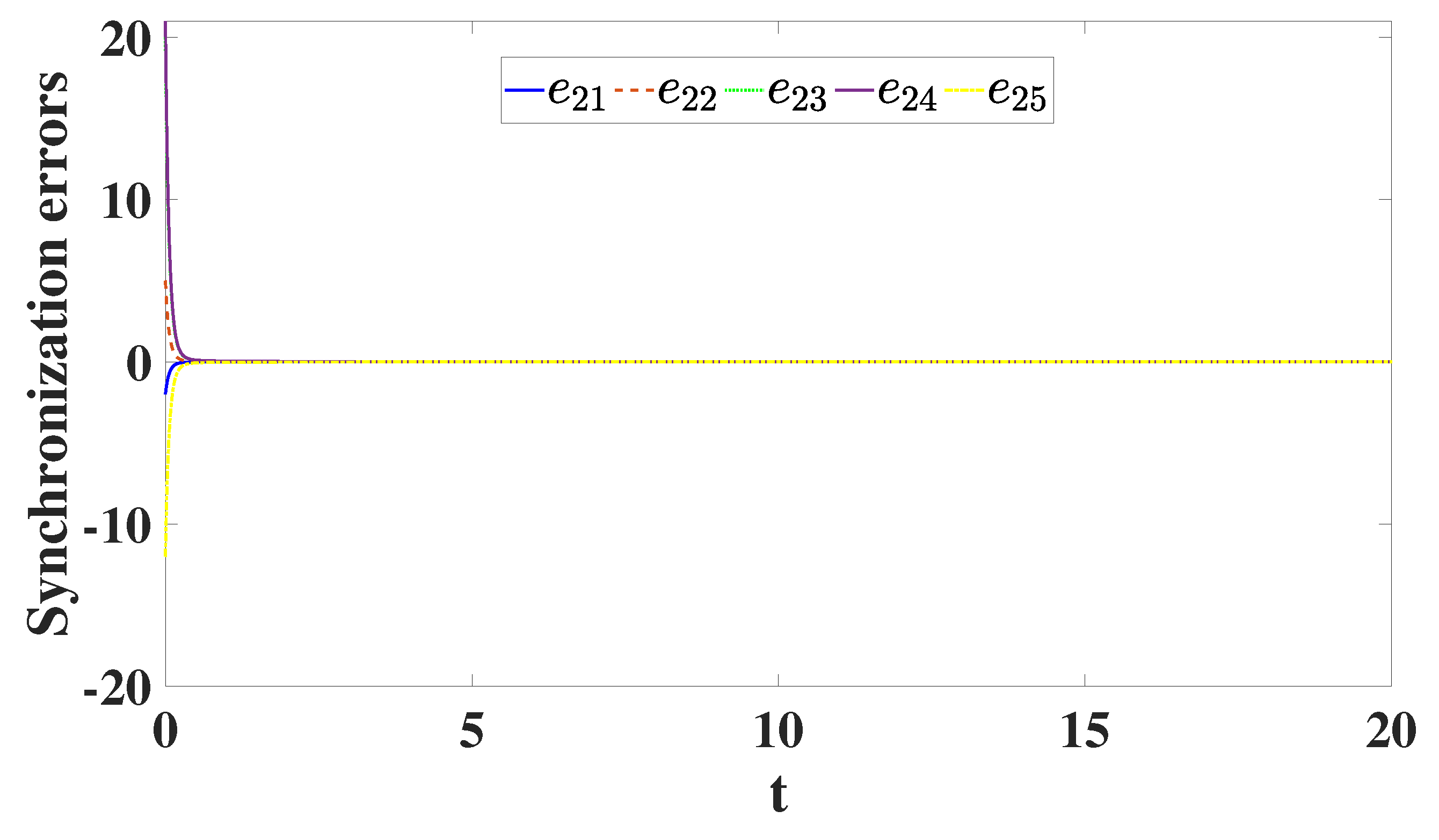
. Selecting , , and , the results of DCS of models (6.17–6.19) are depicted in Figure 8, Figure 9, Figure 10 and Figure 11. The three dimensional projection in the first two drive models of (6.17-6.18) and the first one response model of (6.19) are plotted in Figure 8: space and space. In addition, the three dimensional projection in the second two drive models of (6.17-6.18) and second response model of (6.19) are indicated in Figure 9: space and space. This shows that the DCS is performed as suggested by Theorem 6.1. As shown in Figure 10 and Figure 11, on the other hand, the synchronization errors e converge to zero very rapidly as .
7. Conclusions
We have examined the dynamical properties of the proposed DOHD laser model (1.4), including dissipation, invariance, and studied its FPs and the coexistence of a hyperchaotic attractor. We have shown that this model has a hyperchaotic attractor and a circle of FPs. The observation of multiple coexisting behaviours demonstrates that this hyperchaotic model has multistability, with: chaotic and hyperchaotic attractors and solutions that approach the FP as seen in Figure 5, Figure 6 and Figure 7, respectively. In the domain where our model (1.4) has solutions that approach FPs, we find that choosing different initial conditions does not affect the type of solutions in the corresponding intervals. We also obtained solutions that approach FPs for all different choices of initial conditions. Other choices of our initial conditions in different intervals can be similarly studied. We introduced the Definition 3 of DCS for two DO response models and four integer-order drive models. Remarks 6.1-6.2 state that this definition is considered as a generalization of those found in the literature. Furthermore, we introduced a scheme to achieve DCS. The formula for the analytical control function to achieve DCS is obtained by Theorem 6.1. Examples are provided to illustrate the great agreement among the numerical and analytical results, see Figure 8, Figure 9, Figure 10 and Figure 11. With respect to the Caputo derivative, the outcomes are largely consistent with those of the DO method, except when is very close to 1 from below. In that case, the system stills tends to a chaotic attractor. For all other values of , both the Caputo and DO approaches lead to a rapid convergence to the fixed point.
Supplementary Materials
The following supporting information can be downloaded at the website of this paper posted on Preprints.org.
Funding
No funds, grants, or other support was received.
Conflicts of Interest
The authors declare that they have no conflict of interest concerning the publication of this manuscript.
References
- Caputo, M. Elasticita e dissipazione; Bologna: Zanichelli, 1969. [Google Scholar]
- Caputo, M. Mean fractional-order-derivatives differential equations and filters. Annali dell’Universita di Ferrara 1995, 41, 73–84. [Google Scholar] [CrossRef]
- Caputo, M. Distributed order differential equations modelling dielectric induction and diffusion. Fractional Calculus and Applied Analysis 2001, 4, 421–442. [Google Scholar]
- Bagley, R.; Torvik, P. On the existence of the order domain and the solution of distributed order equations-Part I. International Journal of Applied Mathematics 2000, 2, 865–882. [Google Scholar]
- Bagley, R.; Torvik, P. On the existence of the order domain and the solution of distributed order equations-Part II. International Journal of Applied Mathematics 2000, 2, 965–988. [Google Scholar]
- Fernández-Anaya, G.; Nava-Antonio, G.; Jamous-Galante, J.; Muñoz-Vega, R.; Hernández-Martínez, E. Asymptotic stability of distributed order nonlinear dynamical systems. Communications in Nonlinear Science and Numerical Simulation 2017, 48, 541–549. [Google Scholar] [CrossRef]
- Mahmoud, G.M.; Aboelenen, T.; Abed-Elhameed, T.M.; Farghaly, A.A. Generalized Wright stability for distributed fractional-order nonlinear dynamical systems and their synchronization. Nonlinear Dynamics 2019, 97, 413–429. [Google Scholar] [CrossRef]
- Mahmoud, G.M.; Farghaly, A.A.; Abed-Elhameed, T.M.; Aly, S.A.; Arafa, A.A. Dynamics of distributed-order hyperchaotic complex van der Pol oscillators and their synchronization and control. The European Physical Journal Plus 2020, 135, 1–16. [Google Scholar] [CrossRef]
- Mahmoud, G.M.; Khalaf, H.; Darwish, M.M.; Abed-Elhameed, T.M. Synchronization and desynchronization of chaotic models with integer, fractional and distributed-orders and a color image encryption application. Physica Scripta 2023, 98, 095211. [Google Scholar] [CrossRef]
- Tomovski, Ž.; Sandev, T. Distributed-order wave equations with composite time fractional derivative. International Journal of Computer Mathematics 2018, 95, 1100–1113. [Google Scholar] [CrossRef]
- Abed-Elhameed, T.M.; Mahmoud, G.M.; Elbadry, M.M.; Ahmed, M.E. Nonlinear distributed-order models: Adaptive synchronization, image encryption and circuit implementation. Chaos, Solitons & Fractals 2023, 175, 114039. [Google Scholar]
- Aboelenen, T. Local discontinuous Galerkin method for distributed-order time and space-fractional convection–diffusion and Schrödinger-type equations. Nonlinear dynamics 2018, 92, 395–413. [Google Scholar] [CrossRef]
- Chen, J.; Li, C.; Yang, X. Chaos Synchronization of the Distributed-Order Lorenz System via Active Control and Applications in Chaotic Masking. International Journal of Bifurcation & Chaos in Applied Sciences & Engineering 2018, 28. [Google Scholar]
- Zeghlache, H.; Mandel, P. Influence of detuning on the properties of laser equations. Journal of the Optical Society of America B 1985, 2, 18–22. [Google Scholar] [CrossRef]
- Ning, C.z.; Haken, H. Detuned lasers and the complex Lorenz equations: subcritical and supercritical Hopf bifurcations. Physical Review A 1990, 41, 3826. [Google Scholar] [CrossRef]
- M. Mahmoud, G.; Bountis, T.; Al-Kashif, M.; Aly, S.A. Dynamical properties and synchronization of complex non-linear equations for detuned lasers. Dynamical Systems 2009, 24, 63–79. [Google Scholar] [CrossRef]
- Mahmoud, G.M.; Abed-Elhameed, T.M.; Khalaf, H. Synchronization of hyperchaotic dynamical systems with different dimensions. Physica Scripta 2021, 96, 125244. [Google Scholar] [CrossRef]
- Li, X.; Mou, J.; Banerjee, S.; Wang, Z.; Cao, Y. Design and DSP implementation of a fractional-order detuned laser hyperchaotic circuit with applications in image encryption. Chaos, Solitons & Fractals 2022, 159, 112133. [Google Scholar]
- Feudel, U. Complex dynamics in multistable systems. International Journal of Bifurcation and Chaos 2008, 18, 1607–1626. [Google Scholar] [CrossRef]
- Ngonghala, C.N.; Feudel, U.; Showalter, K. Extreme multistability in a chemical model system. Physical Review E 2011, 83, 056206. [Google Scholar] [CrossRef]
- Bao, B.; Li, Q.; Wang, N.; Xu, Q. Multistability in Chua’s circuit with two stable node-foci. Chaos: An Interdisciplinary Journal of Nonlinear Science 2016, 26, 043111. [Google Scholar] [CrossRef]
- Lai, Q.; Chen, S. Coexisting attractors generated from a new 4D smooth chaotic system. International Journal of Control, Automation and Systems 2016, 14, 1124–1131. [Google Scholar] [CrossRef]
- Chen, Y.M. Dynamics of a Lorenz-type multistable hyperchaotic system. Mathematical Methods in the Applied Sciences 2018, 41, 6480–6491. [Google Scholar] [CrossRef]
- Bao, B.; Bao, H.; Wang, N.; Chen, M.; Xu, Q. Hidden extreme multistability in memristive hyperchaotic system. Chaos, Solitons & Fractals 2017, 94, 102–111. [Google Scholar]
- Jin, M.; Sun, K.; Wang, H. Dynamics and synchronization of the complex simplified Lorenz system. Nonlinear Dynamics 2021, 106, 2667–2677. [Google Scholar] [CrossRef]
- Zhou, W.; Wang, G.; Iu, H.; Shen, Y.; Liang, Y. Complex dynamics of a non-volatile memcapacitor-aided hyperchaotic oscillator. Nonlinear Dynamics 2020, 100, 3937–3957. [Google Scholar] [CrossRef]
- Mahmoud, G.M.; Aboelenen, T.; Abed-Elhameed, T.M.; Farghaly, A.A. On boundedness and projective synchronization of distributed order neural networks. Applied Mathematics and Computation 2021, 404, 126198. [Google Scholar] [CrossRef]
- Mahmoud, G.M.; Abed-Elhameed, T.M.; Khalaf, H. On fractional and distributed order hyperchaotic systems with line and parabola of equilibrium points and their synchronization. Physica Scripta 2021, 96, 115201. [Google Scholar] [CrossRef]
- Yang, L.x.; He, W.s.; Liu, X.j. Synchronization between a fractional-order system and an integer order system. Computers & Mathematics with Applications 2011, 62, 4708–4716. [Google Scholar] [CrossRef]
- Diethelm, K.; Ford, N.J.; Freed, A.D. A predictor-corrector approach for the numerical solution of fractional differential equations. Nonlinear Dynamics 2002, 29, 3–22. [Google Scholar] [CrossRef]
- Wolf, A.; Swift, J.B.; Swinney, H.L.; Vastano, J.A. Determining Lyapunov exponents from a time series. Physica D: Nonlinear Phenomena 1985, 16, 285–317. [Google Scholar] [CrossRef]
- Mahmoud, G.M.; Ahmed, M.E.; Abed-Elhameed, T.M. On fractional-order hyperchaotic complex systems and their generalized function projective combination synchronization. Optik 2017, 130, 398–406. [Google Scholar] [CrossRef]
- Jiao, Z.; Chen, Y.; Podlubny, I. Distributed order dynamic systems, modeling, analysis and simulation; Berlin: Springer, 2012. [Google Scholar]
- Yu, J.; Hu, C.; Jiang, H.; Fan, X. Projective synchronization for fractional neural networks. Neural Networks 2014, 49, 87–95. [Google Scholar] [CrossRef]
- Wang, X.; Zhang, X.; Ma, C. Modified projective synchronization of fractional-order chaotic systems via active sliding mode control. Nonlinear Dynamics 2012, 69, 511–517. [Google Scholar] [CrossRef]
- Mahmoud, G.M.; Mahmoud, E.E. Complex modified projective synchronization of two chaotic complex nonlinear systems. Nonlinear Dynamics 2013, 73, 2231–2240. [Google Scholar] [CrossRef]
- Mahmoud, G.M.; Mahmoud, E.E. Complete synchronization of chaotic complex nonlinear systems with uncertain parameters. Nonlinear Dynamics 2010, 62, 875–882. [Google Scholar] [CrossRef]
Figure 1.
Chaotic attractors for the fractional order detuned laser model (1.3) for , space.
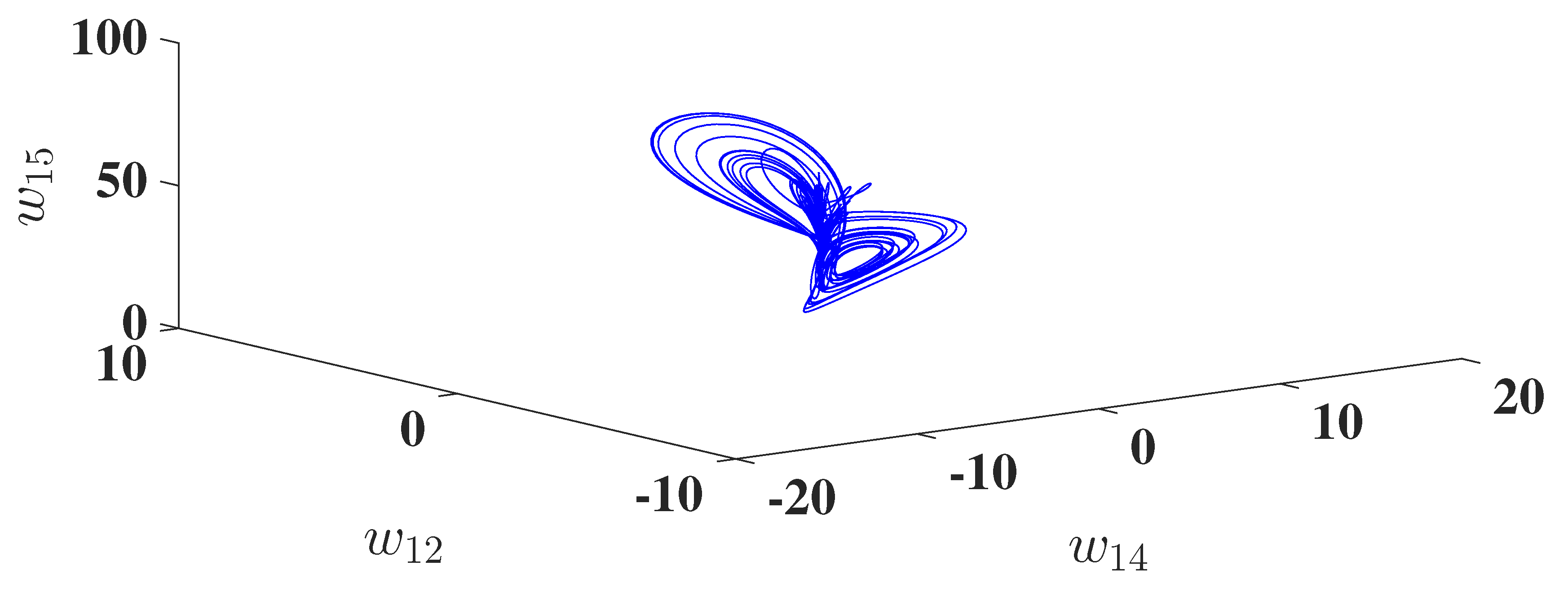
Figure 2.
Chaotic attractors for the fractional order detuned laser model (1.3) for , space.
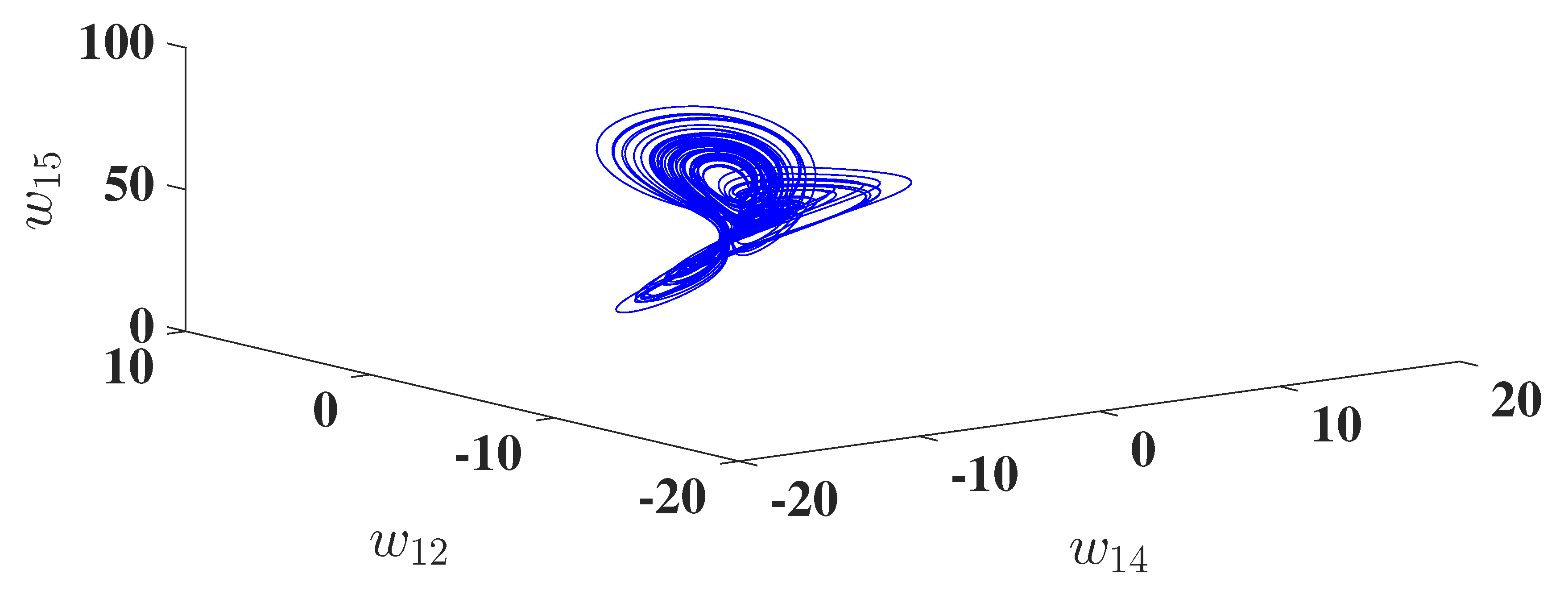
Figure 3.
LEs of the DOHD laser model (1.4), versus t, versus t, , and versus t.
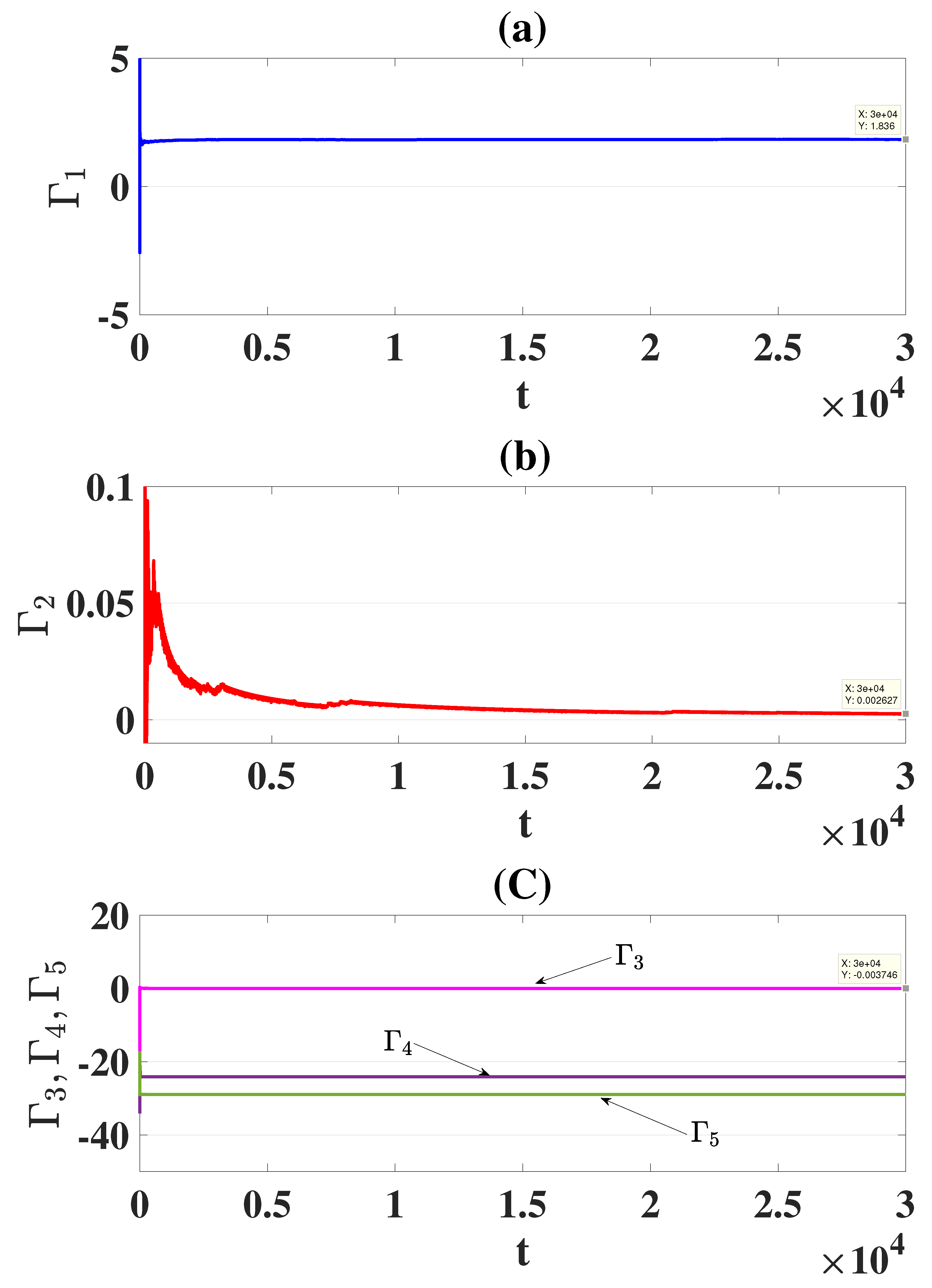
Figure 4.
hyperchaotic attractors for the DOHD laser model (1.4) for , space and space.
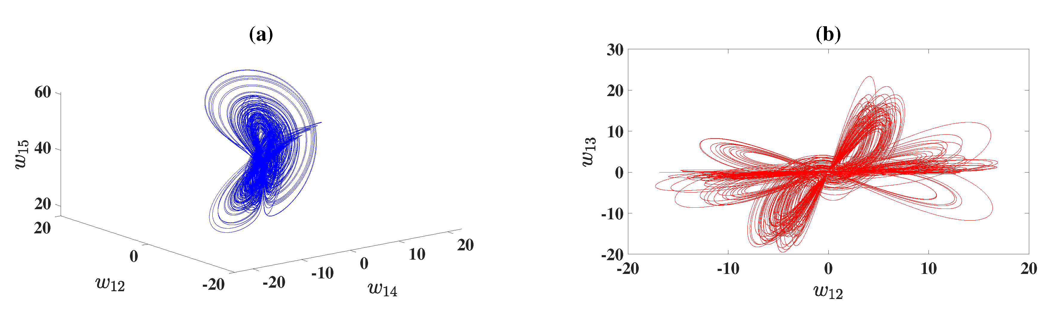
Figure 5.
LEs of model (1.4) for , versus , versus , and versus .
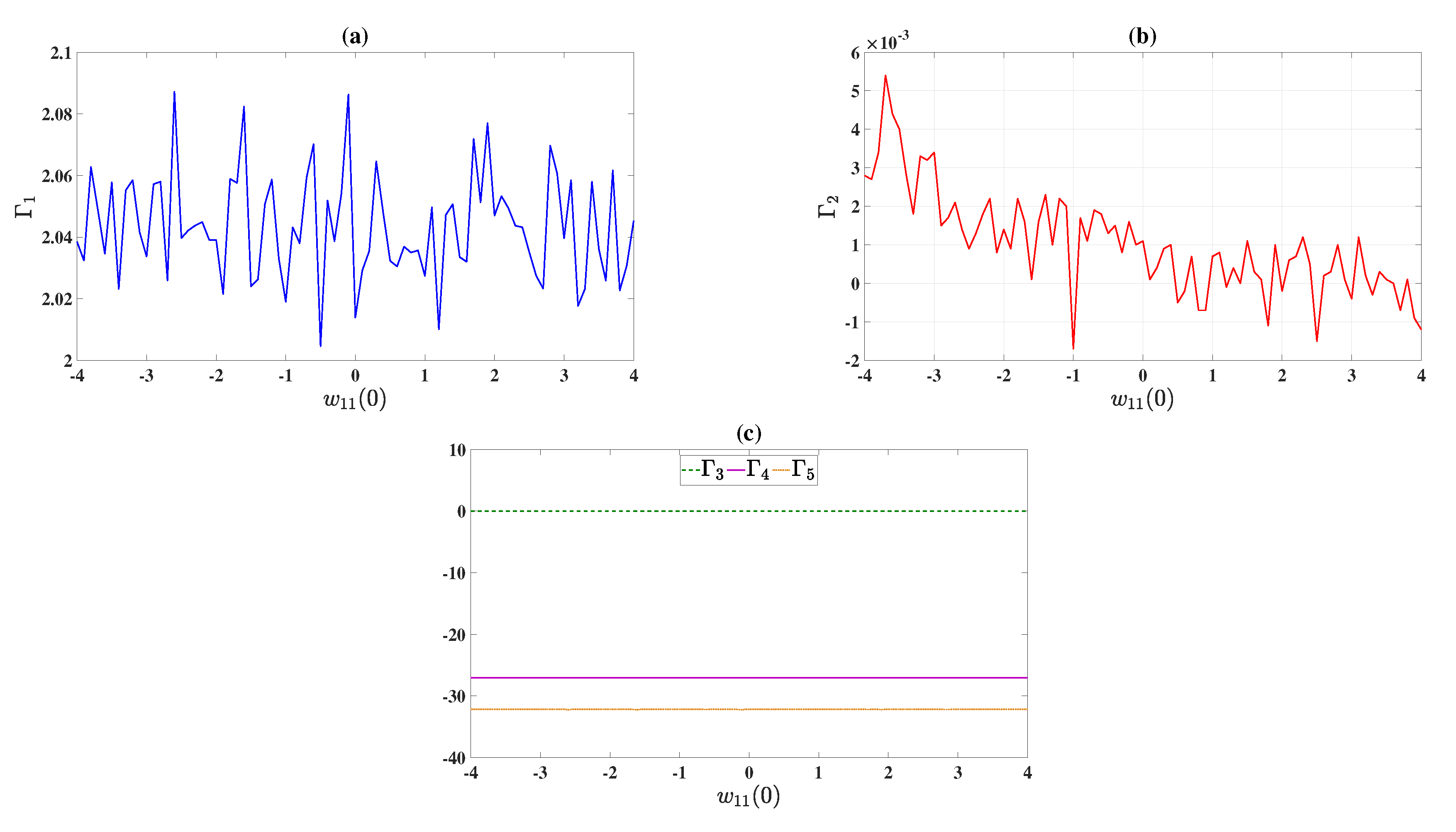
Figure 6.
Different coexisting attractors of model (1.4) for and different initial conditions and on space and space.
Figure 6.
Different coexisting attractors of model (1.4) for and different initial conditions and on space and space.
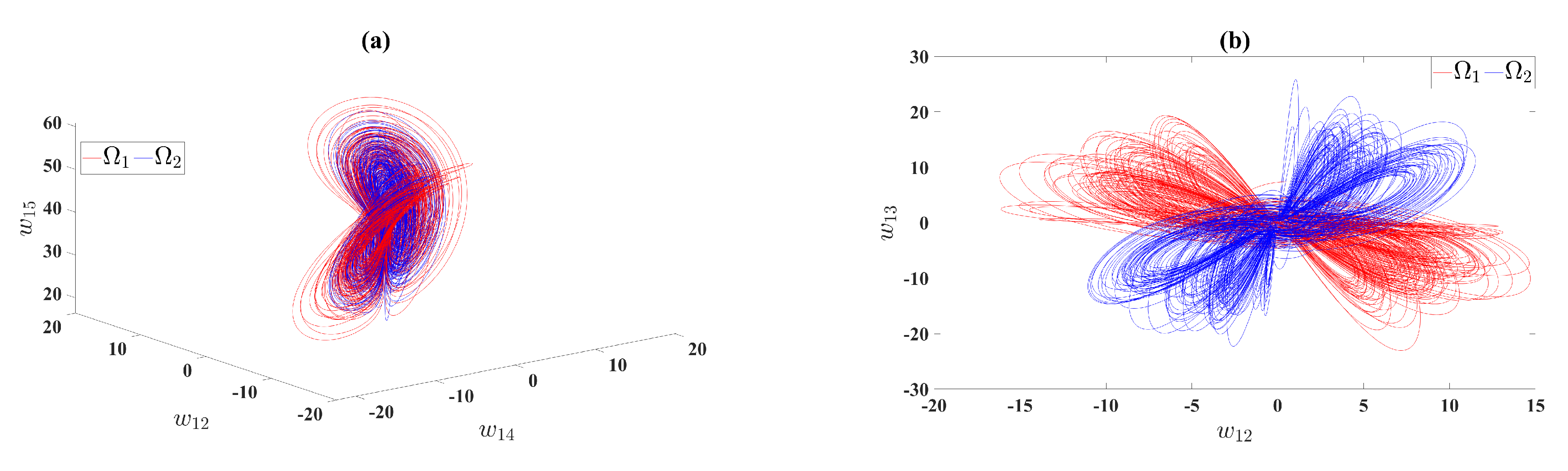
Figure 7.
Solution that approaches FPs of the DOHD laser model (1.4) for and the initial condition , space and space.
Figure 7.
Solution that approaches FPs of the DOHD laser model (1.4) for and the initial condition , space and space.
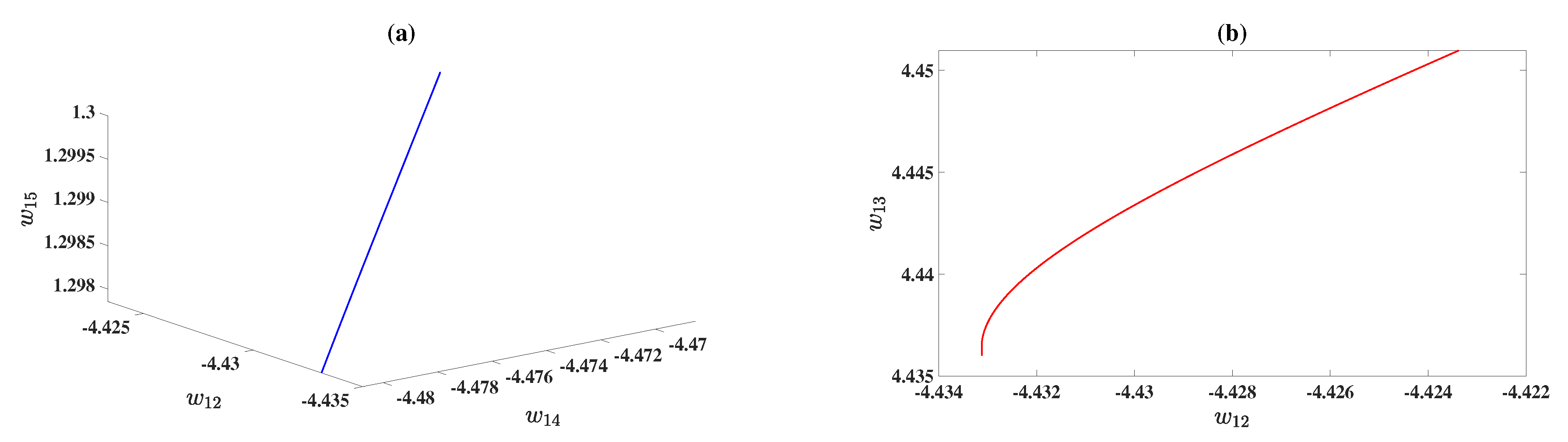
Figure 8.
DCS of: the first two drive models of (6.17-6.18) in space and the first response model of (6.19) in space.
Figure 8.
DCS of: the first two drive models of (6.17-6.18) in space and the first response model of (6.19) in space.
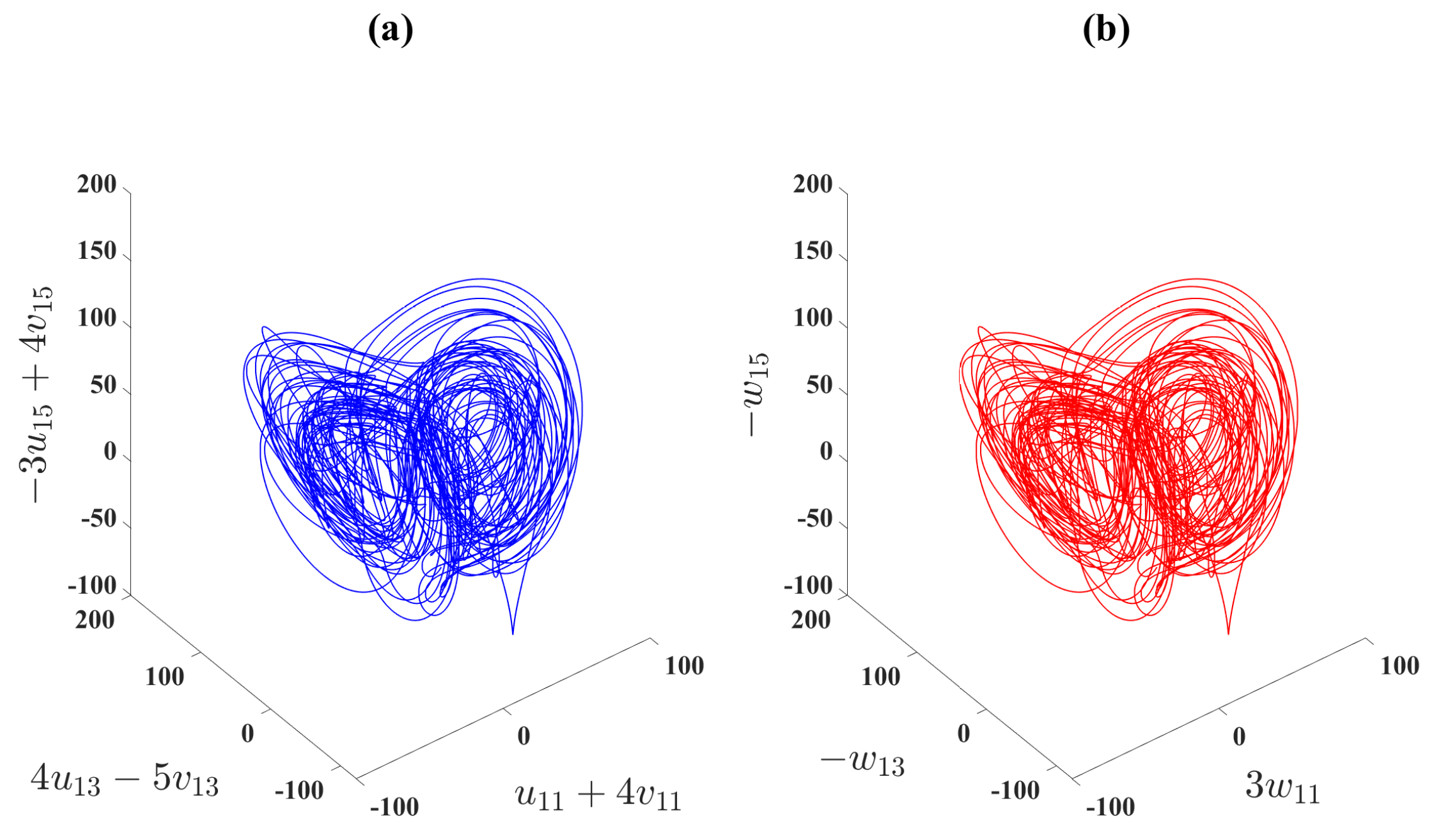
Figure 9.
DCS of: the second two drive models of (6.17-6.18) in space and the second response model of (6.19) in space.
Figure 9.
DCS of: the second two drive models of (6.17-6.18) in space and the second response model of (6.19) in space.
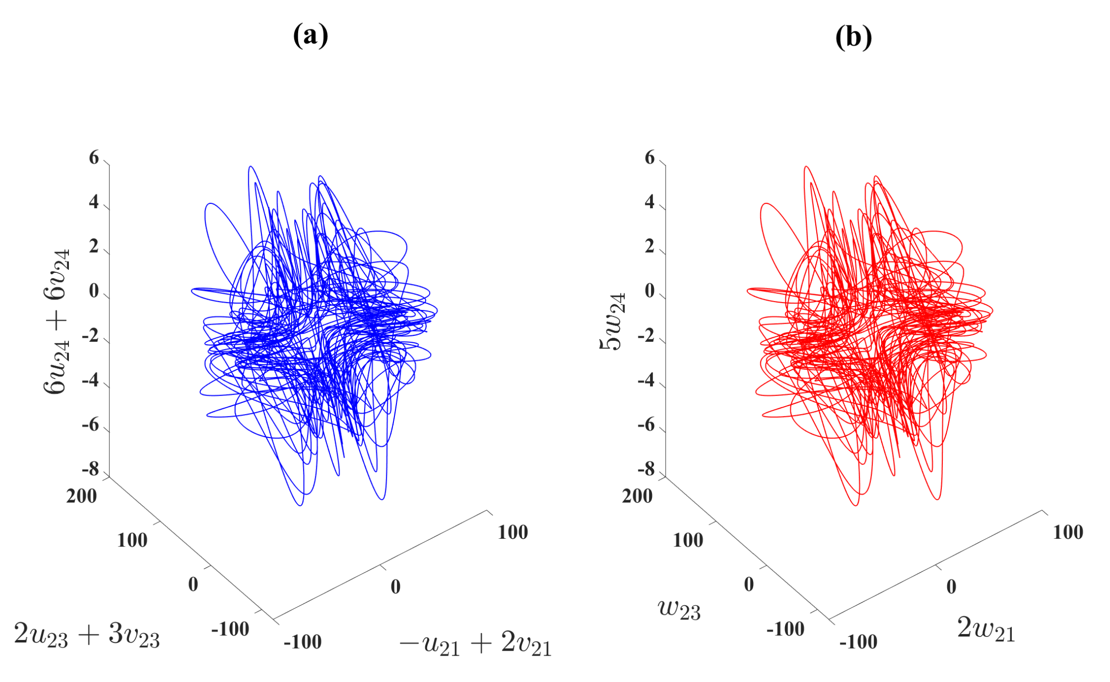
Figure 10.
Synchronization errors for the first two drive models of (6.17-6.18) and the first one response model of (6.19) versus t, (solution of the model (6.21) for ).
Figure 10.
Synchronization errors for the first two drive models of (6.17-6.18) and the first one response model of (6.19) versus t, (solution of the model (6.21) for ).
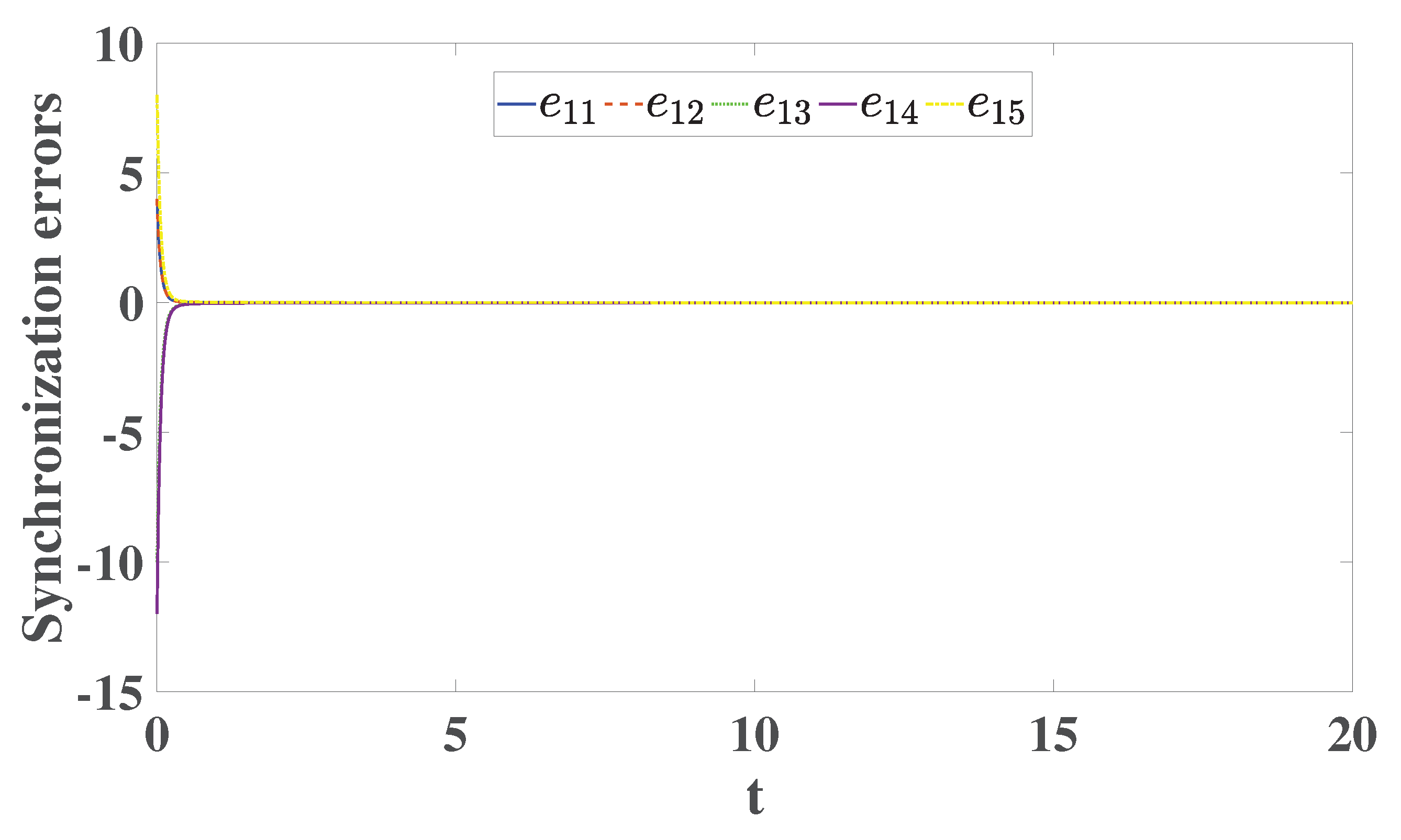
Figure 11.
Synchronization errors for the second two drive models of (6.17-6.18) and the second one response model of (6.19) versus t, (solution of the model (6.21) for ).
Figure 11.
Synchronization errors for the second two drive models of (6.17-6.18) and the second one response model of (6.19) versus t, (solution of the model (6.21) for ).
Disclaimer/Publisher’s Note: The statements, opinions and data contained in all publications are solely those of the individual author(s) and contributor(s) and not of MDPI and/or the editor(s). MDPI and/or the editor(s) disclaim responsibility for any injury to people or property resulting from any ideas, methods, instructions or products referred to in the content. |
© 2025 by the authors. Licensee MDPI, Basel, Switzerland. This article is an open access article distributed under the terms and conditions of the Creative Commons Attribution (CC BY) license (http://creativecommons.org/licenses/by/4.0/).
Copyright: This open access article is published under a Creative Commons CC BY 4.0 license, which permit the free download, distribution, and reuse, provided that the author and preprint are cited in any reuse.


