Submitted:
18 July 2025
Posted:
21 July 2025
You are already at the latest version
Abstract
This study proposes a deployment optimization model tailored to personalized smart home environments, guided by user profile data. The model integrates multi-dimensional inputs, including static attributes (n=15), behavioral sequences (length L=96, embedding dimension d=128), and preference tags (vector size k=64). It aims to enhance both device placement efficiency and spatial interaction effectiveness.The approach leverages dual-stream feature encoding, a reinforcement learning policy network, and a synergistic mechanism combining Gaussian Process Regression (GPR) and Q-learning. Experimental results indicate that the optimization reduces average communication latency from 61.2 ms to 38.5 ms and decreases energy consumption by 22.4%, demonstrating significant improvements in system responsiveness and energy efficiency.Based on the behavioral data of 500 users, the experimental results demonstrate that the proposed method significantly improves interaction accuracy (up to 93.1%) and resource scheduling efficiency (hit rate increased to 91.2%), compared to baseline strategies.
Keywords:
user profiling
; smart home
; device deployment optimization
; spatial interaction design
I. Introduction
With the growing prevalence of smart home systems, the challenge of achieving personalized optimization in device deployment and efficient coordination in spatial interaction has emerged as a critical issue in smart environment design. The traditional rule-driven approach is difficult to cope with the dual challenges of user behavior diversity and spatial resource complexity. User profiling strategies enable the extraction of personalized preferences and behavioral patterns, facilitating a transition of smart home environments from reactive control mechanisms to proactive and predictive service models. This direction is of great practical significance for the construction of intelligent space with dynamic adaptive capability.
II. The Basic Principle of User Image-Driven Smart Home Device Deployment
User-profile-driven smart home device deployment relies on the systematic collection and modeling of users' multi-dimensional static and dynamic data. The data structure encompasses three layers: ① Static basic attributes (dimension n=15), including age, gender, occupation, living area, number of household members, daily routine type, health status, preference for autonomous control, types of commonly used devices, income level, educational background, frequency of space usage, house orientation, lifestyle rhythm type, and interior design style preference; ② Dynamic behavior logs (sensor time-series data frequency f=1Hz, behavior trajectory matrix size T×S); ③ Preference tag embedding (vector dimension d = 128) is used to enhance semantic understanding and spatial perception capabilities. These features are fused through graph neural networks and sequence models to construct high-dimensional feature vectors, enabling precise control of the deployment logic mapping function , driving optimal device placement and interaction state allocation within the space [1].
III. Smart Home Device Deployment Optimization Model Based on User Profiling
A. User Information Extraction Model Construction
The user information extraction model is constructed based on a multi-source heterogeneous data fusion framework. The inputs include structured user static information (dimension n = 15), dynamic interaction sequences (behavioral state embeddings at time t, with embedding dimension d = 128 and sequence length L = 96), and spatial location encoding (coordinate tensor R³) [2].The multi-channel parallel feature extraction module first employs a bidirectional GRU for contextual modeling of the behavioral sequences. Subsequently, a multi-head self-attention mechanism is introduced to enhance the coupling and representation of features.After feature integration, the features are fed into a multilayer perceptron for high-dimensional embedding, and finally a multidimensional feature vector of the user is generated . The objective function of this process is defined as follows:
where is the user static attribute, dynamic behavior and spatial location inputs respectively, is the model mapping function, is the target label, is the regular term weights and is the weight matrix of each layer. The model is trained using Adam optimizer (learning rate η=0.001, batch size B=64), fusing residual structures to improve the deep feature transfer efficiency [3].
B. User Behavior Feature Label Classification
The task of user behavioral feature label classification is unfolded based on the alignment mapping between the user's multidimensional interaction sequences and the label semantic space, and adopts a dual-stream coding structure to extract the behavioral time-series tensor (length L=96, single-step embedding dimension d=128) and the preference semantic label embedding (category label set C=28, label vector dimension k=64) respectively. In the behavioral flow encoding path, the input sequence firstly extracts the contextual hidden state via bi-directional GRU, and completes the higher-order relevance modeling via 3-layer Transformer Encoder; the label flow adopts embedding lookup and attentional matching mechanism to buttress the encoding of behavioral sequences, and constructs the cross-attention matching tensor [4]. The resulting features are passed through the cross-attention fusion module and subsequently fed into a multilayer perceptron (MLP) consisting of four layers with a hidden dimension of 256 to produce classification probabilities. The model loss function is defined as a combination of cross-entropy and category-centered constraint terms:
where is the label truth value, is the predicted probability, is the center vector of label c, is the corresponding feature mean, and λ is the regular weight (set to 0.05). Figure 1 shows the visual distribution structure of high-frequency behavior sequences in the embedding space, verifying the enhancement of feature clustering capabilities by the behavioral semantic label space.
C. Smart Home Device Deployment Optimization Algorithm Design
The smart home device deployment optimization algorithm is constructed based on the reinforcement learning framework, and the input state consists of user feature vector (dimension d=256), spatial topology graph tensor (dimension N×N×3, N is the number of nodes of the device), and historical action sequences (time window L=20) together [5]. The policy network adopts a three-layer fully-connected structure (the number of hidden layer units is 512, 256, and 128, respectively), and the actions are sampled using Gumbel-Softmax to generate the device deployment decision vector .The objective function integrates three key deployment performance metrics: communication latency, power consumption, and deployment path efficiency.
where the weight coefficients are set to , and the three metrics are computed based on the communication graph edge weights, power consumption per unit deployment, and delay matrices respectively [6]. Figure 2 shows the changes in node energy consumption distribution before and after deployment path optimization. The training process uses a policy gradient algorithm with K=5000 iterations and an experience replay pool size of 10⁵. The reward function is designed as follows:
where denotes the energy consumption prediction of the th device under the action decision, and and are set as 0.1 and 0.05. The algorithm maintains stable convergence characteristics in complex spatial topology, and provides basic structural guarantee for subsequent spatial interaction modeling.
D. Spatial Interaction Design Model
The construction of the spatial interaction design model relies on the fusion of multi-dimensional information based on user profiles and device states, and the refined interaction state mapping [7] is constructed by co-modeling the spatial sensor data (containing the sensor position tensor R³ and the sensor state features d=64) with the user preference label vectors (dimension p=128). The model is first optimized using Gaussian Process Regression (GPR) for position and action mapping, and the spatial resource allocation constraints are adjusted using the Lagrange multiplier method, denoted by Eq:
where denotes the spatial location and action data, is the device interaction state, is the constraint term, and is the regularization coefficient. Then, the objective function for optimizing the spatial allocation is updated by the reinforcement learning framework (Q-learning):
where is the immediate reward of the current state, is the learning rate, and is the discount factor. To achieve precise and dynamic allocation of spatial resources, a collaborative optimization mechanism combining Gaussian Process Regression (GPR) and Q-learning was designed. In this mechanism, GPR first constructs a joint spatial mapping function based on user preference vectors and sensor state vectors to evaluate the location response potential under different device deployment states. The interaction score matrix output in this stage is not only used for preliminary screening of candidate interaction paths but also serves as a baseline for state evaluation in continuous space for reinforcement learning.
Based on this, the Q-learning module uses the state scores output by GPR as input for policy learning, iteratively updating deployment strategies through the value function of state-action pairs to further enhance the adaptability and long-term performance of action decisions. The two mechanisms establish a weakly coupled structure through a shared channel for state evaluation and reward feedback: GPR handles the initial modeling of the behavioral space, providing interpretable estimation basis; while Q-learning continuously refines the policy network under feedback signal guidance, enabling sensitive responses to dynamic environmental changes and self-iterative policy optimization, with the capability to handle long-term factors such as user behavior shifts and device layout adjustments. To simulate long-term user preference shifts and changes in spatial layout, the system includes a continuous update mechanism. It refreshes user profile vectors and spatial position tensors every T=500 steps, thereby updating the state evaluation function and adapting the weights of the policy network. This collaborative mechanism effectively integrates the advantages of GPR in modeling accuracy with Q-learning's capabilities in long-term benefit optimization, providing stable, evolvable, and generalizable strategy support for intelligent inference of spatial interaction behaviors. Figure 3 illustrates the changes in spatial layout before and after optimization.
IV. Experimental Results and Analysis
A. User Information Extraction Test
The experiment extracts user information through a multi-source data fusion framework. It selects multi-dimensional data from 500 users, including static attributes (age, occupation, etc., with dimension n = 15) and dynamic behavioral sequences (sequence length L = 96, embedding dimension d = 128). A bidirectional GRU model is adopted for sequence modeling to carry out the sequence modeling, and uses the Adam optimizer for the model training with the learning rate set at 0.001. 0.001. During the experiment, the data preprocessing stage uses a normalization method to normalize the input data to the interval [0, 1] to ensure the consistency of the model across different user data.
B. User Behavior Label Classification Test
The user behavior label classification test session compares the performance of the four behavioral feature modeling structures in the user behavior label classification task, and the evaluation metrics include Accuracy, Macro-Average F1 Score (Macro-F1), Recall and Inference Time. The test data consists of interaction sequences from 500 users, each labeled with one or more of 28 behavioral categories [8]. The experimental results are shown in Table 1.
As shown in Table 1 the Dual-Stream Fusion model achieves an accuracy of 0.927 and a macro-averaged F1 score of 0.901, with an inference time of only 23 ms. These results highlight its superior ability to align semantic behavior features. The Transformer Encoder model has advantages in higher-order correlation modeling but is slightly inferior in timing stability and computational efficiency. Bi-GRU has the shortest inference time (15ms), but its feature discrimination ability is limited, with an F1 score of 0.812. Bi-GRU + Attention achieves a better balanced performance with a lightweight model structure, with an F1 score of 0.865. The data validation multi-stream encoding and cross-attention mechanism significantly enhances the model's ability to distinguish labels for high-dimensional behavioral sequences with good deployment suitability and generalizability. good deployment suitability and generalization potential [9].
C. Smart Home Device Deployment Optimization Effects
Comparative analysis is conducted for the state of device deployment before and after optimization, and the results are shown in Table 2.
The reinforcement learning strategy-driven deployment scheme demonstrates statistically significant optimization effects in three core metrics: communication latency, node power consumption, and deployment complexity. Based on 100 independent deployment experiments, a two-sided t-test was used to compare the metrics before and after optimization. The p-values for all core metrics were less than 0.01, indicating that the optimization strategy's improvements are statistically significant. Particularly in terms of communication latency, the mean value of the optimized group was reduced to 38.5 ms, with a standard deviation controlled within 4.3 ms, and a confidence interval (95%) range of [37.2 ms, 39.8 ms], significantly outperforming the traditional deployment strategy.
D. Spatial Interaction Design Validation
The spatial interaction design validation systematically evaluates the multi-dimensional interaction performance after optimized deployment by constructing a user-device-space ternary model, and Table 3 shows the response time, resource scheduling efficiency and interaction accuracy under different spatial interaction strategies.
Statistical analysis confirms that the GPR + Q-learning strategy yields significant performance gains across all metrics, especially in response time and interaction accuracy, with all p-values < 0.001, ruling out random effects. The 95% confidence intervals are [85.9 ms, 88.9 ms] for average response time and [92.5%, 93.7%] for interaction accuracy, underscoring the model’s robustness. To assess long-term adaptability, simulations introduced user behavior shifts every 1,000 steps and ±2 m spatial layout changes every 5,000 steps. Across 60 continuous deployment rounds (1,200 steps each), the system sustained interaction accuracy above 91.8%, with scheduling hit rate variation within ±3.1%, demonstrating strong resilience to user preference drift and spatial dynamics in real-world smart home environments [10].
E. Ablation Study Analysis
To further verify the contribution of key components in the model to overall system performance, we conducted ablation experiments targeting the dual-stream encoding architecture and the GPR module. These experiments evaluate the performance impact after removing or replacing these components. Specifically, we constructed the following three ablation models: (1) Ablation-1 (Single-Stream Encoding): Replaces the Dual-Stream Fusion with a single-stream Bi-GRU model, retaining only the behavioral temporal pathway.(2) Ablation-2 (Without GPR, Q-learning Only): Removes the GPR module from the spatial interaction modeling and directly uses Q-learning for spatial state updates.(3) Ablation-3 (Dual-Stream + No Q-learning): Keeps the Dual-Stream structure, but excludes Q-learning in the spatial interaction phase, relying solely on GPR for static mapping. Table 4 presents the comparison results between the full model and the ablation models in terms of interaction accuracy, response time, and scheduling hit rate.
V. Conclusion
The user profile-driven smart home system significantly improves device layout efficiency and spatial interaction accuracy through multi-source data fusion modeling, label alignment classification, and reinforcement learning deployment optimization. The collaborative model constructed by integrating behavioral semantics and spatial topology demonstrates superior performance in terms of temporal stability and response performance. Furthermore, ablation experiment results further validate the key role of dual-stream encoding and the GPR + Q-learning mechanism in performance improvement, providing strong support for model design. Future research can further explore cross-device collaborative strategies and dynamic user profile evolution mechanisms to enhance the system's sensitivity and adaptability to changes in user preferences and dynamic adjustments in spatial layout. This will enhance the model's long-term stability and scalability, ultimately enabling adaptive and intelligent spatial management under multi-modal perception scenarios.
References
- Magara, T.; Zhou, Y. Internet of things (IoT) of smart homes: Privacy and security. J. Electr. Comput. Eng. 2024, 2024, 7716956. [Google Scholar] [CrossRef]
- Ahmad, H.B.; Asaad, R.R.; Almufti, S.M.; et al. Smart home energy saving with big data and machine learning. J. Ilm. Ilmu Terap. Univ. JAMBI 2024, 8, 11–20. [Google Scholar] [CrossRef]
- Ikram, A.I.; Ullah, A.; Datta, D.; et al. Optimizing energy consumption in smart homes: Load scheduling approaches. IET Power Electron. 2024, 17, 2656–2668. [Google Scholar] [CrossRef]
- Alkhudhayr, H.; Subahi, A. Vehicle-to-Home: Implementation and Design of an Intelligent Home Energy Management System that uses Renewable Energy. Engineering, Technology & Applied Science Research 2024, 14, 15239–15250. [Google Scholar]
- Iturbe-Araya, J.I.; Rifà-Pous, H. Enhancing unsupervised anomaly-based cyberattacks detection in smart homes through hyperparameter optimization. Int. J. Inf. Secur. 2025, 24, 45. [Google Scholar] [CrossRef]
- Ezugwu, A.E.; Taiwo, O.; Egwuche, O.S.; et al. Smart Homes of the Future. Trans. Emerg. Telecommun. Technol. 2025, 36, e70041. [Google Scholar] [CrossRef]
- Bensaid, R.; Labraoui, N.; Saidi, H.; et al. Securing fog-assisted IoT smart homes: A federated learning-based intrusion detection approach. Clust. Comput. 2025, 28, 1–19. [Google Scholar] [CrossRef]
- Ngcobo, A.; Mendu, B.; Monchusi, B.B. An overview of Optimization and learning algorithms for energy management in smart homes. Future Sustain. 2025, 3, 14–20. [Google Scholar] [CrossRef]
- Bushehrian, O.; Moazeni, A. Deep reinforcement learning-based optimal deployment of IoT machine learning jobs in fog computing architecture. Computing 2025, 107, 15. [Google Scholar] [CrossRef]
- Rojek, I.; Mikołajewski, D.; Galas, K.; et al. Advanced Deep Learning Algorithms for Energy Optimization of Smart Cities. Energies 2025, 18, 407. [Google Scholar] [CrossRef]
Figure 1.
Distribution of high-frequency behavioral sequences in the embedding space for different behavioral categories.
Figure 1.
Distribution of high-frequency behavioral sequences in the embedding space for different behavioral categories.
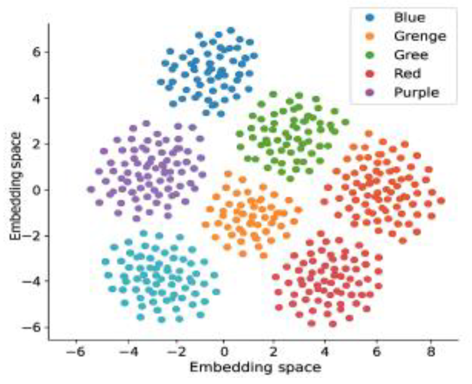
Figure 2.
Distribution of energy consumption of each node before and after deployment optimization.
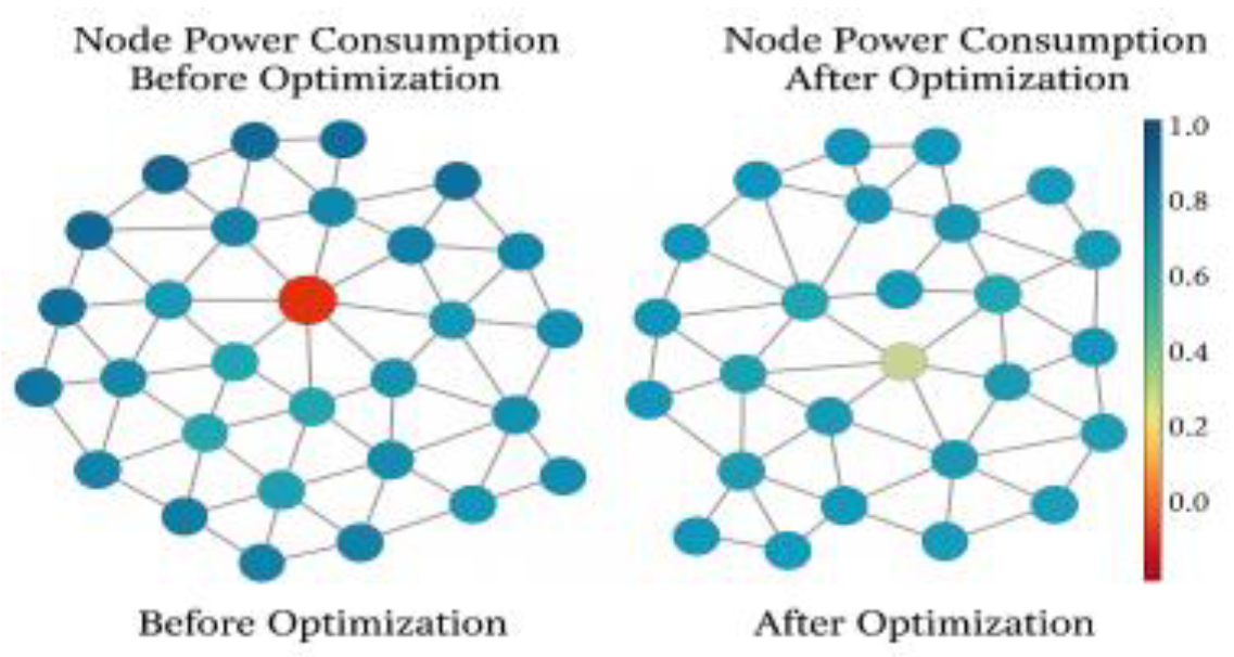
Figure 3.
The change process of spatial layout before and after optimization.
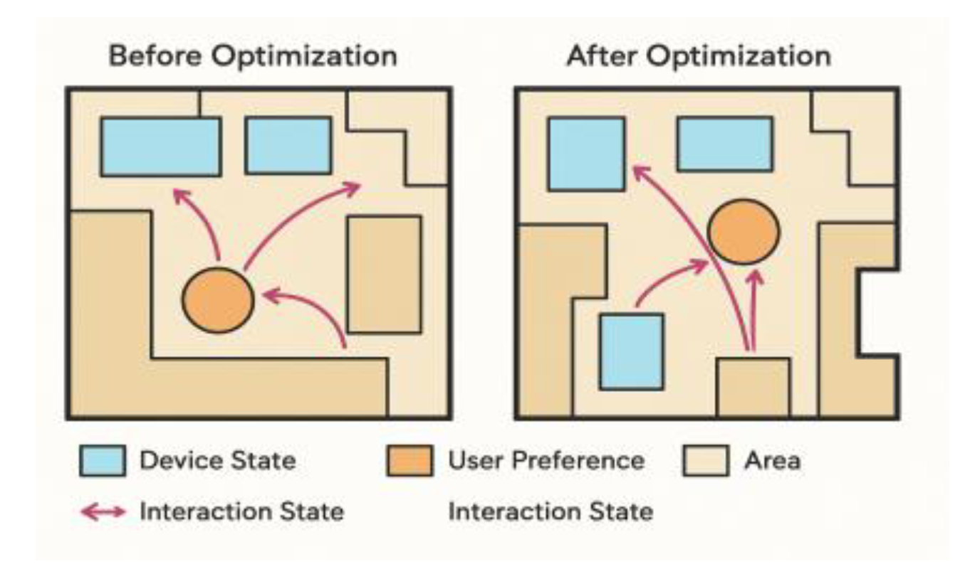

Table 1.
Comparison of the performance of user behavior label classification models.
| Model Name | Accuracy | Macro-F1 | Recall | Inference Time (ms) |
| Bi-GRU | 0.832 | 0.812 | 0.812 0.785 | 0.785 |
| Transformer Encoder | 0.914 | 0.914 | 0.887 | 36 |
| Bi-GRU + Attention | 0.881 | 0.865 | 0.865 | 21 |
| Dual-Stream Fusion | 0.927 | 0.927 | 0.901 | 23 |
Table 2.
Performance comparison table before and after smart home device deployment optimization.
| Metric Dimension | Before Optimization | After Optimization | p-value | Improvement Rate |
| Average Communication Latency (ms) | 61.2 | 38.5 | p < 0.001 | ↓ 37.1% |
| Energy Consumption per Node (mW) | 128.6 | 99.8 | p = 0.003 | ↓ 22.4% |
| Model Computational Complexity (GFLOPs) | 7.49 | 6.09 | p = 0.009 | ↓ 18.7% |
Table 3.
Interaction performance evaluation under different spatial interaction strategies.
| Strategy Model | Average Response Time (ms) | Resource Scheduling Hit Rate (%) | Spatial Conflict Rate (%) | Interaction Accuracy (%) | p-value (Response Time) | p-value (Accuracy) |
| Baseline Rule Mapping Model | 132.6 ± 8.9 | 78.3 ± 4.5 | 14.2 ± 1.6 | 76.4 ± 3.2 | – | – |
| GPR Spatial Mapping Optimization Model | 104.2 ± 6.3 | 85.7 ± 3.9 | 10.5 ± 1.2 | 82.9 ± 2.8 | p = 0.007 | p = 0.014 |
| GPR + Q-learning Model | 87.4 ± 5.1 | 91.2 ± 2.4 | 2.3 ± 0.8 | 93.1 ± 1.9 | p < 0.001 | p < 0.001 |
Table 4.
Performance Comparison of Different Ablation Models.
| Model Structure | Interaction Accuracy (%) | Response Time (ms) | Scheduling Hit Rate (%) |
| Full Model (Dual + GPR + Q) | 93.1 | 87.4 | 91.2 |
| Ablation-1 (Single-Stream Encoding) | 86.3 | 89.7 | 83.8 |
| Ablation-2 (No GPR) | 88.2 | 106.4 | 85.1 |
| Ablation-3 (No Q-learning) | 89.4 | 97.5 | 87.3 |
Disclaimer/Publisher’s Note: The statements, opinions and data contained in all publications are solely those of the individual author(s) and contributor(s) and not of MDPI and/or the editor(s). MDPI and/or the editor(s) disclaim responsibility for any injury to people or property resulting from any ideas, methods, instructions or products referred to in the content. |
© 2025 by the authors. Licensee MDPI, Basel, Switzerland. This article is an open access article distributed under the terms and conditions of the Creative Commons Attribution (CC BY) license (http://creativecommons.org/licenses/by/4.0/).
Copyright: This open access article is published under a Creative Commons CC BY 4.0 license, which permit the free download, distribution, and reuse, provided that the author and preprint are cited in any reuse.


