Submitted:
16 July 2025
Posted:
21 July 2025
You are already at the latest version
Abstract
Microglia are central to neuroimmune responses and undergo dynamic structural and functional changes in models of stress and addiction, and in response to pharmacological treatments. While transcriptomic and proteomic assays provide insights into molecular profiles, morphological analysis remains a valuable proxy for assessing region-specific microglial response. However, morphological features alone often fail to capture the full complexity of microglial function, underscoring the need for standardized methods and complementary approaches. Here, we describe a standardized imaging pipeline for ana-lyzing microglia in the nucleus accumbens core (NAcore), integrating unbiased confocal image acquisition with precise anatomical reference points. We compare two widely used image analysis platforms—IMARIS and CellSelect-3DMorph—highlighting their work-flows, output metrics, and utility in quantifying microglial morphology following treat-ment with adenosine triphosphate (ATP). Both tools detect well described features of mi-croglial dynamics, though they differ in automation level, analysis speed, and output types. Our findings demonstrate that both platforms provide reliable morphological data, with CellSelect-3DMorph offering a rapid, open-access alternative for high-throughput analysis. Additionally, using software-derived parameters in principal component analy-sis clustering has proven useful for identifying distinct subpopulations of microglia sepa-rated by their morphology. This work provides a practical framework for morphological analysis and promotes reproducibility in microglial studies under environmental and pharmacological interventions.
Keywords:
microglia
; morphology
; neuroimmune
; analysis
1. Introduction
Microglia are the primary immune cells of the central nervous system (CNS) and play critical roles in maintaining neural homeostasis, responding to injury, and shaping synaptic networks. In neuropsychiatric contexts, such as stress and substance use disorders, microglia exhibit dynamic changes in both form and function[1].Accurately characterizing these changes is essential for understanding their contributions to neuropathology. Recent literature emphasizes the need for multimodal approaches that integrate diverse data types to define microglial states more precisely and avoid overreliance on single-assay interpretations [2].
Among the techniques available for assessing microglial function, three major categories are widely utilized: transcription-based assays (transcriptomics), protein-based assays (proteomics), and morphological analyses [3,4,5,6,7]. Morphological analysis provides a valuable complementary approach, especially in in-vivo and ex-vivo models. Traditionally, microglia exhibiting highly ramified processes have been interpreted as homeostatic, while amoeboid (reduced ramification) forms suggest a reactive, pro-inflammatory phenotype [8,9]. However, emerging evidence reveals that microglial morphology spans a spectrum of forms that do not always align with functional activation states. As such, morphological analysis should be seen as an important—but incomplete—proxy for function [2] .
To maximize the interpretability and reproducibility of morphological studies, standardization of image acquisition and analysis protocols is essential. In this manuscript, we describe a standardized confocal imaging pipeline for analyzing microglia in the nucleus accumbens (NAc), specifically in the nucleus accumbens core (NAcore)—a region critically involved in reward, stress response, and addiction pathology. We detail an unbiased imaging method based on anatomical reference points and high-resolution 3D confocal microscopy, followed by comparison of two widely used morphological analysis platforms: IMARIS (Oxford Instruments), a commercial 3D visualization and reconstruction tool, and CellSelect-3DMorph, an open-access, MATLAB-based semiautomated analysis suite developed in our laboratory[10].
By highlighting methodological strengths, limitations, and analytic outputs of both platforms, we aim to provide researchers with a clear framework for selecting appropriate tools and interpreting morphological data within broader multimodal investigations. Moreover, we aim to achieve a comprehensive understanding of microglial morphological analysis, by furthering our understanding of morphology with principal component analysis (PCA) and two-step clustering, using the parameters provided by the CellSelect-3DMorph. Clustering analysis is a tool that aids in identifying different populations within the microglia present in a brain region; hence providing a better understanding of how experimental manipulations affect the neuroimmune system. However, while morphology alone cannot define microglial function, robust morphological assessment remains a critical component in the integrative analysis of microglial dynamics under stress and addiction-like conditions.
2. Materials and Methods
2.1. Animals
All housing and experimental procedures were conducted in accordance with the Medical College of Wisconsin Institutional Animal Care and Use Committee (IACUC) regulations. Animals were double or triple housed in the Biomedical Resource Center in a 12-hour inverted light cycle prior to experimental manipulation. Eight female Long-Evans rats used in the experiment had ad libitum access to standard chow and water for the duration of the study. These rats were divided into two groups and given intraperitoneal injections of either adenosine 5’-triphosphate (ATP; n=4; disodium salt, Millipore Sigma, A7699-1G) or saline vehicle (VEH; n=4). Following the injections, rats returned to their home cages for two hours. ATP was administered at a dose of 50 mg/kg, as described in [11]. Two hours after the injections, the animals were perfused, and tissue was collected.
2.2. Immunostaining
For the immunohistochemical staining, rats were intracardially perfused with 4% paraformaldehyde, followed by an overnight post-fixation period. Brains were sliced the following day at 100 um thickness. The tissue was stained with a macrophage and microglia marker: ionized calcium binding adaptor molecule 1 (rabbit anti-IBA-1 1:300; Invitrogen PA5-21274) primary antibody for morphological analysis. Free floating brain slices were washed 3 times for 5 min in 1x phosphate buffer saline (PBS); followed by a permeabilization in 1x PBS + 0.5% triton (PBST; Thermo scientific A16046.AP) for 10 minutes. The brains were then incubated for 1 hour in a blocking solution consisting of 5% Normal goat serum (Invitrogen, PI31873) + 0.5% PBST at room temperature. After blocking step, brain slices were incubated in the blocking solution + rabbit anti-IBA-1 antibody 24 hours at 4C on a shaker. After the primary antibody step, brains slices were washed 3 times for 10 minutes with 0.1% PBST, followed by a 2-hour incubation in secondary antibody Alexa 568, goat anti-rabbit (1:200, Thermofisher. A78955) at room temperature covered from light. The tissue was then washed 3 times in 1x PBS before mounting and cover slipping the tissue. Brain slices were mounted onto charged microscope slides and air dried before cover slipping with mounting media (Invitrogen, ProLong Gold antifade mountant, P36930).
2.3. Data Analysis
All data analyses were done using GraphPad Prism 10 software(Boston, MA), where all data sets were first tested for D’Agostino & Pearson normality test before further analysis. The microglial morphological data has been shown to not be normally distributed. Therefore, we performed a nonparametric analysis on these data via a Mann-Whitney U for two group rank-comparisons and Kolmogorov Smirnov distribution comparison. Sholl analysis data were analyzed with a mixed model analysis. The clustering analysis was done with SPSS software and then further analyzed with GraphPad software. The clustered microglia morphology data was normally distributed, therefore, was analyzed using ordinary ANOVA analysis when appropriate, as well as observing the multiple comparisons using Bonferroni’s post-hoc testing.
3. Results
3.1. Microglial Morphology: Applications and Limitations in Neuroimmune Research
Growing interest in how diverse cell types may interact in a physical manner (i.e., structural changes) to promote functional changes in brain circuits has ignited our interest in exploring and refining approaches to study cellular morphology. Due to the heterogeneity of structure among different cell types, our current approach specifically targets microglia. Many platforms exist for the detection and subsequent classification of cellular morphology. However, they range in their ability to capture various aspects of microglial morphology, with the amount of information gathered limited by a balance between throughput and detail. Here, we demonstrate the use of Cell Select-3DMorph, a high-throughput method for characterizing microglial morphology that retains high fidelity offered by three-dimensional analyses.
The following sections contain discussion of techniques for image acquisition, morphometric processing, and data analyses, that can be applied to study microglia morphology. Through rigorous investigation of microglial morphology in models of health and disease, we aim to appreciate the consequential, and often nuanced, role of these cells in the development and persistence of neuropsychiatric disease.
3.2. Unbiased Image Acquisition Methodology
Morphological analyses rely heavily on image quality, resolution, and unbiased acquisition from a region of interest. The NAc is a subcortical brain structure known primarily for its roles in motivated behavior and as a motor-limbic interface that mediates goal-directed behaviors [12,13,14]. A subregion within the NAc, the NAcore, undergoes long-lasting synaptic plasticity in response to chronic use of addictive drugs [12,15] (e.g., heroin, cocaine, alcohol, nicotine) and stress exposure [16,17,18,19,20,21].
Microglia visualization is required to perform morphological studies, commonly using IBA-1, a cytoplasmic calcium binding protein expressed in microglia and macrophages, as a marker [22]. For the purposes of this manuscript, we refer to all IBA-1 + cells as microglia. Furthermore, there are other markers for microglia, including CD11b, CX3CR1, and CD68. Alternatively, TMEM119 and P2Y12R are markers that are exclusive for microglia. Additionally, multiple transgenic reporter lines are constructed by genetically inserting a fluorescent marker gene sequence to a gene of interest (e.g. CX3CR1GFP, TMEM119GFP, Sall1GFP), this insertion causes the addition of the fluorescent marker into the target protein [23,24,25]. However, these are typically mouse lines. Currently, the only transgenic rat construct available is a cre recombinase-dependent CX3CR1-ERT2 line (Rat Resource & Research Center, Columbia, MO). IBA-1 is a good morphological marker, as the protein is distributed throughout microglial cytoplasm, thus enabling clear visualization. As a result, it has been extensively utilized as a microglial marker in various mammalian models, including rodents, non-human primates, and rabbits [26].
For a precise morphological analysis, it is important to visualize microglial cells with most, if not all, of their projections in the field of view. Therefore, 3D analyses of microglia are preferred over 2D analyses, for which the full cell is not assessed. To achieve 3D images, thick brain sections are recommended, as they enable comprehensive imaging of the microglia. For this purpose, we recommend sectioning the brain into 100-μm slices. However, others have demonstrated that sufficient 3D morphological characteristics in microglia can be observed with 50-μm sections[27]. Following microglial labeling, confocal microscopy is recommended for image acquisition. Confocal microscopy is preferred for morphological analysis, as it can acquire high-resolution 3D images of cells. Figure 1 shows our unbiased image acquisition methodology in the NAcore using confocal microscopy.
We have developed an unbiased imaging technique to capture our regions of interest using a reference point within the structure to aid imaging. Reference points are important to ensure consistency of imaging locations across groups. We use the anterior commissure (a.c.) as reference point to image the NAcore (Figure 1A). Focusing on the NAcore using the Paxinos Rat Brain Atlas [28] and the work of Voorn et al. [29], we have traced the known glutamatergic projections from the ventral prelimbic cortex, dorsal prelimbic cortex, and dorsal anterior cingulate (PLv, PLd, and ACd, respectively). The NAcore spans an anterior posterior (AP) range from +3.00 to +0.50. Within this range, the rostral NAcore corresponds to AP +3.00 to +1.80, while the caudal NAcore spans from AP +1.80 to +0.50. For each animal, we acquire a total of six images: three from defined positions within the rostral NAcore and three from corresponding positions in the caudal NAcore, as detailed in the following section. The tissue sections and coordinates illustrated in Figure 1 represent the caudal portion of the NAcore.
Once cells are stained and fields are defined in the microscope, confocal imaging can be conducted. Here we describe a protocol using a LeicaX SP8 Upright Confocal Microscope and the LASX software suite. This protocol can be adapted to other microscopes and software configurations. First, we survey brain sections with a 5x objective (or the lowest magnification objective available) to locate the region of interest, positioning it in the center of the field of view. Next, use the 10x objective and set the gain and intensity that allow for the best quality and resolution of the cells across treatment groups. Using a tile stitching function, we perform a spiral scan around the reference point. Then, using the microscope software, we add a mark, the focal point (F), in the center of the reference structure, (Figure 1C – see arrow indicating F). For example, when imaging the NAc, we mark the focal point at the center of the anterior commissure (a.c.). Next, we change the objective to 63x oil immersion magnification. Note that we prefer a 63x objective for optimal resolution and cellular definition for morphological analyses; however others have used a 40x objective [30]. Once the objective is set, using the navigator interface, we create a tile scan grid, (for example: a 12x10 tile scan grid - each square being 0.172 μm by 0.172 μm) with the center of the grid (shown as a cross with a circle) defined by the focal point (F) (Figure 1C). The grid allows coordinates to be set consistent with each image position across groups (Figure 1D); the x,y image position coordinates used within the NAcore are (3,4), (5,8), (9,2) for n1, n2 and n3, respectively. The 3 positions (n1, n2 and n3) were selected because these locations receive different glutamatergic projections (PLv, PLv and ACd respectively). Using consistent grid positions across treatment groups ensures unbiased image collection. Prior to imaging, parameters must be set for ideal resolution and image quality of the cells. We find that some general parameters that yield good resolution images include a resolution of 1024x1024 pixel resolution, a scan speed of 600 Hz, a line average of 3, and a pinhole size of 1μm. Parameters that often may vary between experiments/cohorts include gain and intensity; these parameters often need to be adjusted to achieve a low background image with good resolution of the cell branches. It is important to ensure that the parameters are consistent across the treatment conditions and that the investigator is blinded to the conditions. Lastly, we recommend that the Z-stack step size (distance between photos on the Z-axis) is set at 0.5 μm, as smaller steps are optimal for increased branch resolution. The image presented in Figure 1E has a ~37μm thick Z-stack.
3.3. Morphological Analysis Tool Comparison
Morphological analyses of microglia typically focus on the ramification states of the cells; historically these states have been defined by calculating the quantities and lengths of branches, with more and longer branches indicating more ramified microglia compared to amoeboid microglia, which have fewer and smaller branches [2,33,34]. In the past decades, multiple platforms have been developed for morphological analyses; each with pros and cons, making selection of the proper tool challenging. Prior to selecting an analysis tool, a criterion must be set to include or exclude cells for the analysis. A good criterion for 3D analysis of microglia is to exclude incomplete cells (i.e., cells that have less than 80% of its soma and projections within the xyz planes of the image), as morphology cannot be accurately assessed in those cells. Following criterion selection, an analysis tool must be selected. A commonly used software is IMARIS (Oxford Instruments), as it is capable of 3D analysis.
IMARIS is an application that aids in the visualization of confocal images in 3D and has options that enable reconstruction and measurement of cell morphology and colocalization, as well as protein and cell quantification (in addition to a range of other applications). Here, we will focus on the morphological analysis features of IMARIS. Cell morphology can be analyzed using the IMARIS cell surface and filament functions which reconstruct the cells and define characteristics that relate to morphology. Cell surface creation permits measurement of cell and soma volumes, while filament creation enables measurement of branch endpoints, branchpoints, and branch length (sum), and Sholl analysis-based analysis of branch complexity, among other measures. We recommend using the filament creation function, as it measures more morphological characteristics that allow for accurate analyses compared to the cell surface creation function. Figure 2 presents a stepwise summarized protocol for filament creation in IMARIS. The filament creation function in IMARIS has an automatic system (Figure 2A) by which the soma diameter and fluorescent thresholding are set (Figure 2B). However, the microglial somas must be manually positioned (Figure 2C). Once this is done, IMARIS machine learning will reconstruct the branches of the microglia (Figure 2D). With machine learning, it is possible to teach IMARIS to accurately define branches. IMARIS will store this information in parameter files so that it can be applied to future images. Once the initial reconstruction is complete (Figure 2E), we exclude cells that are not within our criteria (Figure 2F) and eliminate any filaments that are not connected or do not originate from the same cell to obtain our finalized image (Figure 2G). Although IMARIS provides excellent visualization of the cells as well as accurate reconstruction, the time required for this process is high relative to some other platforms.
In 2018, an open access semi-automated microglia analysis platform called 3DMorph was released. The MATLAB-based code had multiple advantages that encouraged us to update and optimize the base code [10]. Since numerous changes were implemented, we renamed and released it as CellSelect-3DMorph 1.0 (10.5281/zenodo.14159877). An important difference between the code and its predecessor [30] is its compatibility with the current version of MATLAB and the release of a standalone executable that does not require a MATLAB license. Additionally, improvements have been made to enhance efficiency, resulting in faster code execution. It also introduces the option to select which cells to analyze and which to exclude. Both free, open-access versions are available on the Garcia-Keller laboratory’s GitHub space (https://github.com/CGK-Laboratory/CellSelect-3DMorph). CellSelect-3DMorph is a semiautomatic software, where the reconstruction of the cells is achieved through automatic reconstruction of the cells based on manual decisions made by the user. Once images are acquired using a confocal microscope (raw image, Figure 3A), an otsu threshold is defined for each image (Figure 3B); this threshold determines the background and foreground fluorescent intensity to enable separation among cells [35]. Next, a noise filter is applied (in the same window). This deletes any small objects that have been created and separated after the otsu thresholding (this number is determined by the user as well). Following thresholding, the software gives the option to choose the largest single cell in the image (Figure 3D). This function serves as a checkpoint step, as otsu separation is not perfect and occasionally combines two or more cells together into one object. Users can identify the largest object defined as a single cell, and the software will use this input to define and exclude any larger objects. Similarly, the software will also identify the smallest object in the image defined as a cell and will discard any smaller objects. Subsequently, the software offers the option of selecting cells that fall within the defined range (Figure 3F). Cells to be used for full analysis are then identified. Finally, a full image reconstruction is made (Figure 3E) based on which a final output is generated, consisting of single cell skeletons and 3D reconstructions (Figure 3G) as well as a table (Microsoft Excel™ spreadsheet) providing all quantified measurements. It is worth mentioning that in the final Excel file, certain parameters—such as branchpoints, endpoints, and average, minimum, and maximum branch lengths—may display a value of zero for some cells. This is likely due to rendering errors in the software, which can stem from hardware or software limitations.
CellSelect-3DMorph will define cell volume, cell territory, ramification index, branchpoints, branch endpoints, average branch length and minimum and maximum branch length. Cell volume refers to the volume of the fluorescent pixels encompassing the cell (Figure 3G.1). Cell territory is the maximum expansion of the cell measured by a polygon surrounding the cell (Figure 3G.2). The ramification index is calculated by territorial volume divided by cell volume. Higher values suggest a more ramified cell, where the maximum projection area significantly exceeds the cell’s volume, while lower values indicate an amoeboid shape, with the projection area closely matching the cell volume. Branchpoints quantify the bifurcating points in process branching (Figure 3G.3 and 3G.4), while endpoints quantify all branches. Branchpoints, branch endpoints, minimum and maximum branch length, and average branch length are measurements of cell complexity which have been traditionally used to assess morphology in an indirect manner. However, they are useful for assessing the complexity of the cell morphology (similar to IMARIS). Both CellSelect-3DMorph and IMARIS are similar in their morphological measurements. However, CellSelect-3DMorph is faster than IMARIS for image analysis and can provide a ramification index measurement, while IMARIS can also provide the volume of the soma. Nonetheless, both analyses are useful for determining microglia morphology.
3.4. Comparison of IMARIS and CellSelect-3DMorph Results
To demonstrate the utility of the software for microglial morphological analysis, we present data analyzed using both tools, highlighting their differences and similarities. The experiment involved artificially stimulating a response from microglia through an intraperitoneal injection of adenosine 5’-triphosphate (ATP) disodium salt. ATP disodium salt induces a microglia response by activating purinergic receptors, including P2X and P2Y receptor subtypes [36]. This experiment utilized 10-week-old naïve female rats, divided into two groups: one group received intraperitoneal (i.p.) injections of ATP diluted in ultrapure water, while the control group received vehicle (saline) injections. ATP was administered at a dose of 50 mg/kg, a concentration previously shown to activate microglia in rats [37]. Following the injections, rats were returned to their home cages for a period of two hours, after which rodents were perfused, and tissue was collected. Rats were perfused with 4% paraformaldehyde (PFA) followed by a 24-hour post fixation also in 4% PFA (Figure 4A). The nucleus accumbens core was then imaged and analyzed as described in Figure 1, Figure 2 and Figure 3. Figure 4B displays representative images from each condition, including raw images as well as those reconstructed using IMARIS and CellSelect-3DMorph for each group. Given the dynamic nature of microglia, and likely emergence of distinct subpopulations[2,34,38], morphological measurements obtained from both software platforms exhibit non-normal distributions, requiring the use of non-parametric statistical methods for valid analysis. The data were analyzed using the non-parametric Mann–Whitney rank-sum test. To further validate the findings, the Kolmogorov–Smirnov test for cumulative distribution comparison was also applied. Both statistical tests yielded consistent results. Concurrently, the Sholl measurement data satisfied normality assumptions, enabling the use of parametric statistical analysis. Accordingly, a mixed-effects parametric test was applied to assess the Sholl data. The analysis, conducted with each software platform, indicates that ATP treatment reduced ramification, the number of branchpoints and the overall cell size of microglia, compatible with the transition to an amoeboid-like morphology. Specifically, IMARIS analysis (Figure 4C-F) revealed reductions in Sholl intersections, branchpoints, endpoints, and ramification in ATP-treated animals. Similarly, CellSelect-3DMorph analysis (Figure 4G-N) showed decreased cell volume, territory, branch number, and endpoints following ATP exposure. While both tools preserved the observed group differences, CellSelect-3DMorph may offer a higher-throughput option (processing ~6 images per hour) compared to IMARIS. Our findings demonstrate that both IMARIS and CellSelect-3DMorph are suitable for microglia morphology analysis and provide comparable results.
3.5. Cluster Analysis Pipeline
Thus far, we have emphasized the value of microglial morphology as a foundational approach for understanding microglial states, while also acknowledging its limitations. To address some of these limitations, including the fact that morphology alone may not predict function, static imaging fails to capture dynamic behavior, subpopulation complexity is difficult to resolve, and morphological data often exhibit non-parametric distributions, we implemented a cluster analysis pipeline integrating principal component analysis (PCA) followed by two-step clustering. This analytical approach provides a means to identify the underlying subpopulations and quantify their relative abundance across experimental groups. In doing so, this method allows for the detection of shifts or biases in microglial morphological states in response to experimental manipulation, thereby offering deeper insight into microglial dynamics beyond what is possible with traditional single-parameter or group-mean analyses.
Cluster-based analysis of microglial morphology was carried out in three primary steps: data normalization, PCA, and two-step clustering. First, data were normalized using Z-score transformation, calculated as z = (x - μ) / σ, where x is the raw value, μ is the mean, and σ is the standard deviation. This standardization ensures that all variables are on the same scale, enabling effective dimensionality reduction during PCA. For normalization, data were organized in Excel with columns representing morphological parameters and rows corresponding to individual cells, labeled by animal and treatment groups. Z-scores were calculated separately for each parameter on individual sheets. Once normalized, PCA was performed using SPSS to reduce the dataset into a smaller set of uncorrelated variables, the principal components, that capture the majority of variance in the data. This transformation allows for clearer identification of major patterns and relationships among morphological features. We retained parameters that showed strong contributions to the PCA (component loadings ≥ 0.5) for clustering analysis[39,40,41,42]. Subsequently, two-step clustering was performed in SPSS. This algorithm pre-clusters the data and then applies hierarchical clustering to determine the optimal number of clusters based on the selected variables. SPSS uses a log-likelihood distance measure for clustering and evaluates cluster quality using a silhouette coefficient (algorithmic metric assessing the fitness of the data within a cluster), with values ≥ 0.5 indicating good cluster separation[39,40,42].
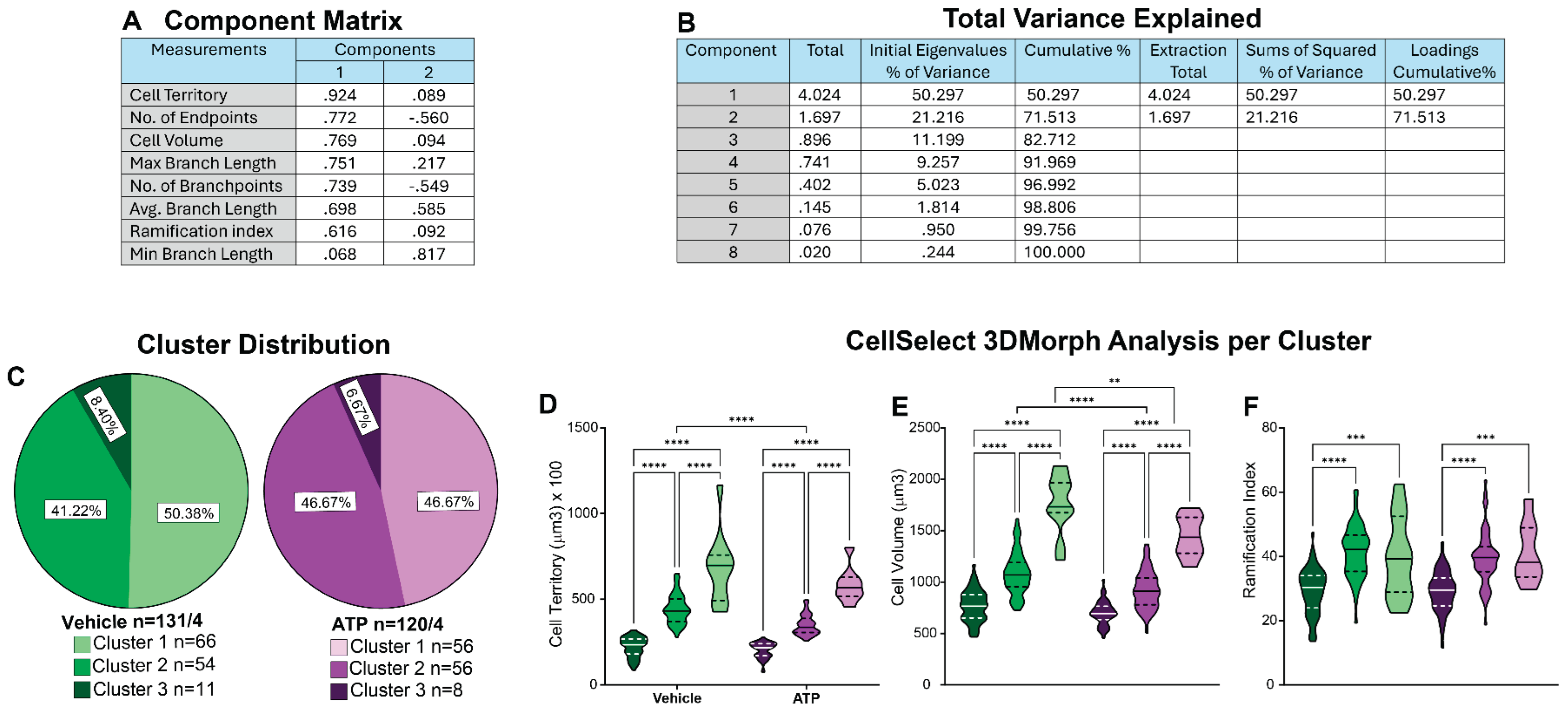
We conducted cluster analysis using CellSelect-3DMorph datasets obtained from both VEH and ATP-treated groups (Figure 4A). All data were pooled and analyzed using the methodology described above. Pooling ensured that cells from both groups were subjected to the same clustering criteria, allowing for unbiased comparison across resulting clusters. To initiate the analysis, all morphological parameters provided by the software including cell territory, cell volume, ramification index, number of branch points, number of endpoints, minimum and maximum branch length, and average branch length, were normalized using Z-score transformation. PCA was then performed to reduce data dimensionality and assess the contribution of each variable. PCA revealed that seven out of the eight parameters demonstrated high quality, indicating they accounted for a substantial portion of the variance in the dataset (Figure 5A), and the first two principal components together explained 71.51% of the total variance (Figure 5B). We initially performed two-step cluster analysis using all seven high-quality parameters. However, this resulted in a cluster quality score of 0.4, which did not meet the threshold for good clustering. This reduced quality was likely due to multicollinearity among parameters, for example, branchpoints and endpoints are highly interrelated. To improve clustering performance, we refined the analysis by selecting three less correlated yet informative parameters: cell territory, cell volume, and ramification index. This revised two-step clustering approach initially yielded two clusters with a silhouette coefficient (cluster quality) of 0.5, indicating acceptable separation. To further capture the dynamic range of microglial states, we applied a three-cluster model, which also achieved a cluster quality of 0.5.
Subsequently, data were stratified by cluster within the VEH and ATP treatment groups for further analysis. Normality tests confirmed that the data within each cluster were normally distributed, allowing for parametric testing. Chi-square analysis was used to compare cluster frequency between groups. Figure 5C shows the microglial population distribution between VEH and ATP groups. Both groups had a comparable distribution, suggesting that that the observed differences in microglial properties (Figure 4) were not attributable to a change in the microglia population composition. Further analysis showed that, within each cluster, in both the VEH and ATP treatment groups, there were significant differences in cell territory and cell volume (Figure 5D-E). Differences in the ramification index were observed between clusters 1 and 2 and between clusters 1 and 3 (Figure 5F). These results suggest that the identified clusters likely represented distinct morphological states that are largely treatment independent. Cluster 1 microglia exhibited the most amoeboid morphology of the dataset, characterized by low cell territory, cell volume, and ramification index. Clusters 2 and 3, while differing significantly in cell territory and cell volume, showed no significant difference in ramification index—likely due to the ramification index being a ratio between cell territory and cell volume parameters. Thus, Cluster 3 represented a more ramified microglial population, whereas Cluster 2 likely reflected either a transitional morphology or a distinct microglial form that does not clearly fall into either the amoeboid or ramified categories. Comparison across treatment groups revealed some notable differences: VEH-treated microglia in Cluster 2 exhibited greater cell territory and volume compared to ATP-treated Cluster 2 cells. Similarly, Cluster 3 microglia in the VEH-treated group had larger cell volumes than their ATP-treated counterparts. These treatment-related differences within clusters may have accounted for the broader morphological changes observed in Figure 4. Collectively, this clustering analysis provides valuable insight into the heterogeneity of microglial responses and enhances our understanding of how ATP treatment influences microglial morphology at the subpopulation level.
4. Conclusions
Morphological analysis, while often used as an indirect measure of microglial activation, provides only a partial view of functional state. Despite its limitations, it remains valuable due to the accessibility of an open-access software, regional specificity within the brain, and compatibility with longitudinal studies (i.e. in-vivo imaging).
To support morphological assessments, we present a standardized confocal imaging protocol centered on anatomical landmarks in the NAcore, ensuring consistent and unbiased image acquisition. We also compare two leading image analysis platforms—IMARIS and CellSelect-3DMorph—demonstrating their strengths, limitations, and comparable performance in detecting microglial morphological changes following ATP-induced activation. IMARIS offers robust 3D reconstructions and versatile analysis tools, albeit with greater time and labor demands. CellSelect-3DMorph, by contrast, is open-source, faster, and semi-automated, offering unique features such as the ramification index.
Importantly, morphological features alone cannot fully define microglial phenotypes or function. The integration of morphological data with clustering analysis provides an opportunity for further interpretations and explanations regarding the morphological changes in microglial populations. However, integrating morphological analyses with transcriptomic and proteomic data is essential for a more comprehensive understanding of microglial responses to stress, drugs, or environmental stimuli. Nevertheless, the standardization of imaging and analysis protocols, combined with validated software tools, represents a critical step toward reproducible and interpretable microglial research in neuropsychiatric and neuroinflammatory models.
Author Contributions
C.G.K. and J.R.M. conceptualized the paper. The methodology used for data analysis was developed by C.G.K., F.J.C and S.W. and the analysis was conducted by C.G.K. and J.P.T. Cluster analysis and discussion was performed by MLA and KAB. The manuscript was prepared, reviewed, and edited by D.B.N., J.P.T., J.R.M., and C.G.K. Funding was provided by C.G.K., J.R.M., and D.B.N. All authors have read and agreed to the published version of the manuscript.
Funding
This research was funded by NIH grants R00 DA047426 to C.G.K., R01 MH136708 and R01 DA059194 to J.R.M. and F30 DA060020 to D.B.N.
Institutional Review Board Statement
Not applicable
Data Availability Statement
The original contributions presented in this study are included in the article material. Further inquiries can be directed to the corresponding authors. The raw data supporting the conclusions of this article will be made available by the authors on request
Acknowledgments
“The views expressed in this publication are those of the authors and do not reflect the official stance of Oxford Instruments America, Inc.”
Conflicts of Interest
The authors declare no conflicts of interest. J.R.M. is a co-founder of Promentis Pharmaceuticals.
References
- Nowak, D.B., et al., Understanding Microglia in Mesocorticolimbic Circuits: Implications for the Study of Chronic Stress and Substance Use Disorders. Cells, 2025. 14(13): p. 1014. [CrossRef]
- Paolicelli, R.C., et al., Microglia states and nomenclature: A field at its crossroads. Neuron, 2022. 110(21): p. 3458-3483. [CrossRef]
- Ball, J.B., et al., Combining RNAscope and immunohistochemistry to visualize inflammatory gene products in neurons and microglia. Frontiers in Molecular Neuroscience, 2023. 16. [CrossRef]
- Schmid, C.D., et al., Differential gene expression in LPS/IFNγ activated microglia and macrophages: <i>in vitro</i> versus <i>in vivo</i>. Journal of Neurochemistry, 2009. 109(s1): p. 117-125.
- Liu, Q.-R., et al., Low Basal CB2R in Dopamine Neurons and Microglia Influences Cannabinoid Tetrad Effects. International Journal of Molecular Sciences, 2020. 21(24): p. 9763.
- Olah, M., et al., Single cell RNA sequencing of human microglia uncovers a subset associated with Alzheimer’s disease. Nature Communications, 2020. 11(1). [CrossRef]
- Kemp, G.M., et al., Sustained TNF signaling is required for the synaptic and anxiety-like behavioral response to acute stress. Mol Psychiatry, 2022. 27(11): p. 4474-4484. [CrossRef]
- Guo, S., H. Wang, and Y. Yin, Microglia Polarization From M1 to M2 in Neurodegenerative Diseases. Frontiers in Aging Neuroscience, 2022. 14.
- Streit, W.J., M.B. Graeber, and W.K. George, Functional plasticity of microglia: A review. Glia, 1988. 1(5): p. 301-307.
- Chaure, F., et al. CellSelect-3Dmorph. [Github Repository] 2023 november 11, 2024.
- Xiang, Y., et al., Adenosine-5’-triphosphate (ATP) protects mice against bacterial infection by activation of the NLRP3 inflammasome. PLoS One, 2013. 8(5): p. e63759.
- Scofield, M.D., et al., The Nucleus Accumbens: Mechanisms of Addiction across Drug Classes Reflect the Importance of Glutamate Homeostasis. Pharmacological Reviews, 2016. 68(3): p. 816-871.
- Turner, B.D., et al., Synaptic Plasticity in the Nucleus Accumbens: Lessons Learned from Experience. ACS Chemical Neuroscience, 2018. 9(9): p. 2114-2126. [CrossRef]
- Everitt, B.J. and T.W. Robbins, Neural systems of reinforcement for drug addiction: from actions to habits to compulsion. Nature Neuroscience, 2005. 8(11): p. 1481-1489.
- Mulholland, P.J., L.J. Chandler, and P.W. Kalivas, Signals from the Fourth Dimension Regulate Drug Relapse. Trends in Neurosciences, 2016. 39(7): p. 472-485.
- Garcia-Keller, C., et al., Behavioral and accumbens synaptic plasticity induced by cues associated with restraint stress. Neuropsychopharmacology, 2021. 46(10): p. 1848-1856. [CrossRef]
- Avalos, M.P., et al., Minocycline prevents chronic restraint stress-induced vulnerability to developing cocaine self-administration and associated glutamatergic mechanisms: a potential role of microglia. Brain, Behavior, and Immunity, 2022. 101: p. 359-376.
- Rigoni, D., et al., Stress-induced vulnerability to develop cocaine addiction depends on cofilin modulation. Neurobiology of Stress, 2021. 15: p. 100349.
- Garcia-Keller, C., et al., Glutamatergic mechanisms of comorbidity between acute stress and cocaine self-administration. Molecular Psychiatry, 2016. 21(8): p. 1063-1069.
- Garcia-Keller, C., et al., Relapse-Associated Transient Synaptic Potentiation Requires Integrin-Mediated Activation of Focal Adhesion Kinase and Cofilin in D1-Expressing Neurons. The Journal of Neuroscience, 2020. 40(44): p. 8463-8477. [CrossRef]
- Fox, M.E., et al., Adaptations in nucleus accumbens neuron subtypes mediate negative affective behaviors in fentanyl abstinence. Biological Psychiatry, 2023.
- Jurga, A.M., M. Paleczna, and K.Z. Kuter, Overview of General and Discriminating Markers of Differential Microglia Phenotypes. Frontiers in Cellular Neuroscience, 2020. 14. [CrossRef]
- Jung, S., et al., Analysis of Fractalkine Receptor CX<sub>3</sub>CR1 Function by Targeted Deletion and Green Fluorescent Protein Reporter Gene Insertion. Molecular and Cellular Biology, 2000. 20(11): p. 4106-4114.
- Kaiser, T. and G. Feng, Tmem119-EGFP and Tmem119-CreERT2 Transgenic Mice for Labeling and Manipulating Microglia. eneuro, 2019. 6(4): p. ENEURO.0448-18.
- Buttgereit, A., et al., Sall1 is a transcriptional regulator defining microglia identity and function. Nature Immunology, 2016. 17(12): p. 1397-1406. [CrossRef]
- Sharma, K., K. Bisht, and U.B. Eyo, A Comparative Biology of Microglia Across Species. Frontiers in Cell and Developmental Biology, 2021. 9.
- Franco-Bocanegra, D.K., et al., Microglial morphology in Alzheimer’s disease and after Aβ immunotherapy. Scientific Reports, 2021. 11(1).
- Paxinos, G. and C. Watson, Paxinos and Watson’s the rat brain in stereotaxic coordinates. Seventh ed. 2014, Amsterdam: Academic Press/Elsevier, 2014.
- Voorn, P., et al., Putting a spin on the dorsal–ventral divide of the striatum. Trends in Neurosciences, 2004. Volume 27(8): p. 468-474. [CrossRef]
- York, E.M., et al., 3DMorph Automatic Analysis of Microglial Morphology in Three Dimensions from<i>Ex Vivo</i>and<i>In Vivo</i>Imaging. eneuro, 2018. 5(6): p. ENEURO.0266-18. [CrossRef]
- Tanaka, K., et al., Prostaglandin E2-mediated attenuation of mesocortical dopaminergic pathway is critical for susceptibility to repeated social defeat stress in mice. J Neurosci, 2012. 32(12): p. 4319-29.
- Bollinger, J.L., et al., Microglial P2Y12 mediates chronic stress-induced synapse loss in the prefrontal cortex and associated behavioral consequences. Neuropsychopharmacology, 2023. 48(9): p. 1347-1357. [CrossRef]
- Reddaway, J., et al., Microglial morphometric analysis: so many options, so little consistency. Frontiers in Neuroinformatics, 2023. 17.
- Sierra, A., R.C. Paolicelli, and H. Kettenmann, Cien Años de Microglía: Milestones in a Century of Microglial Research. Trends in Neurosciences, 2019. 42(11): p. 778-792.
- Otsu, N., A Threshold Selection Method from Gray-Level Histograms. IEEE Transactions on Systems, Man, and Cybernetics, 1979. 9(1): p. 62-66.
- Sáez, P.J., et al., ATP Is Required and Advances Cytokine-Induced Gap Junction Formation in Microglia In Vitro. Mediators of Inflammation, 2013. 2013: p. 1-16. [CrossRef]
- Xiang, Y., et al., Adenosine-5’-triphosphate (ATP) protects mice against bacterial infection by activation of the NLRP3 inflammasome. PLoS One, 2013. 8(5): p. e63759.
- Stratoulias, V., et al., Microglial subtypes: diversity within the microglial community. The EMBO Journal, 2019. 38(17). [CrossRef]
- Mueller, F.S., et al., Behavioral, neuroanatomical, and molecular correlates of resilience and susceptibility to maternal immune activation. Molecular Psychiatry, 2021. 26(2): p. 396-410.
- Zhu, Y., et al., Increased prefrontal cortical cells positive for macrophage/microglial marker CD163 along blood vessels characterizes a neuropathology of neuroinflammatory schizophrenia. Brain Behav Immun, 2023. 111: p. 46-60. [CrossRef]
- Creutzberg, K.C., et al., Vulnerability and resilience to prenatal stress exposure: behavioral and molecular characterization in adolescent rats. Translational Psychiatry, 2023. 13(1). [CrossRef]
- Di Miceli, M., et al., In silico Hierarchical Clustering of Neuronal Populations in the Rat Ventral Tegmental Area Based on Extracellular Electrophysiological Properties. Frontiers in Neural Circuits, 2020. 14.
Figure 1.
Unbiased Confocal Image Acquisition Methodology in the NAcore. An unbiased imaging method was used, capturing tissue at the same three locations across all groups, using the anterior commissure as a reference point. These positions correspond to three distinct areas within the nucleus accumbens core, each associated with different glutamatergic projections. A) Paxinos’s Rat Atlas [28] showing the nucleus NAcore and nucleus accumbens shell (NAshell). B) Mapping of glutamatergic projections onto different zones of the NAc, adapted from [29]. C) Tile scan of the nucleus accumbens at 20x magnification, with the annotated anterior commissure (a.c.), the three positions for image acquisition (n1, n2, n3), and the focal point marked as “F”. D) Numbered gridlines with the drawn anterior commissure (a.c.) illustrating the specific positions of the images within the grid. E) 63x magnification image of microglia in the NAcore at the n1 position.
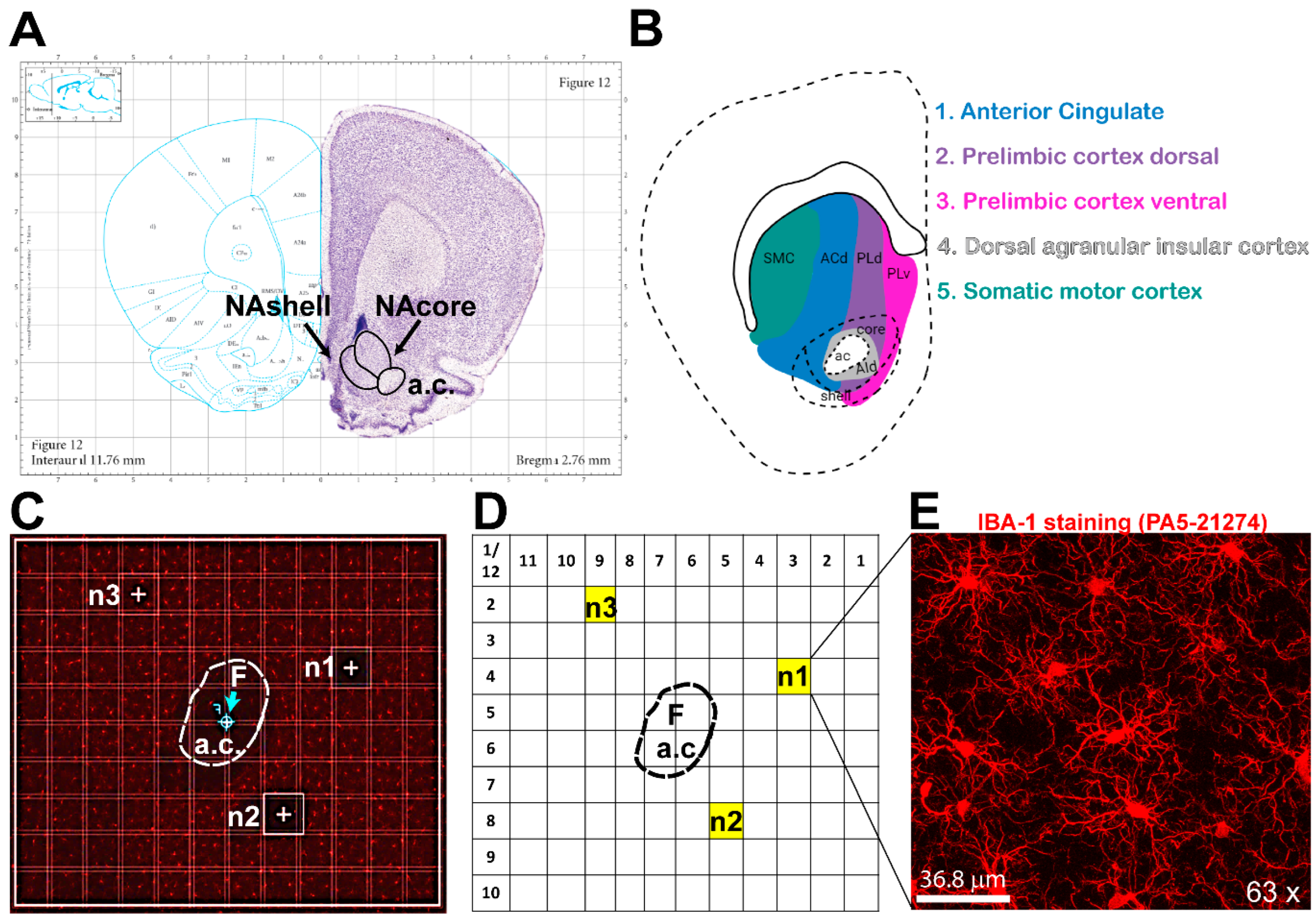
Figure 2.
Microglial Analysis Workflow Using IMARIS Software. The images were analyzed with IMARIS 10.10, utilizing the filament creation function to extract detailed morphological data. A) Begin by selecting the filament creation function and applying the automatic creation option. B) Next, choose the largest diameter of the cells. C) Once the diameter is selected, the software will automatically populate the soma size within the image. D) IMARIS employs machine learning to distinguish between specific and non-specific branching during reconstruction. This step is crucial as the parameters from this machine learning process can be applied to all other images. E) Use volume thresholding to remove small, non-specific projections before completing the reconstruction. F) After reconstruction, remove any incomplete cells whose morphology cannot be accurately measured. G) The final output consists of cells whose morphology can be accurately assessed. H) IMARIS provides a broad range of statistical measurements, with the most relevant for morphological analysis being branch points, branch endpoints, sholl analysis, and soma volume.
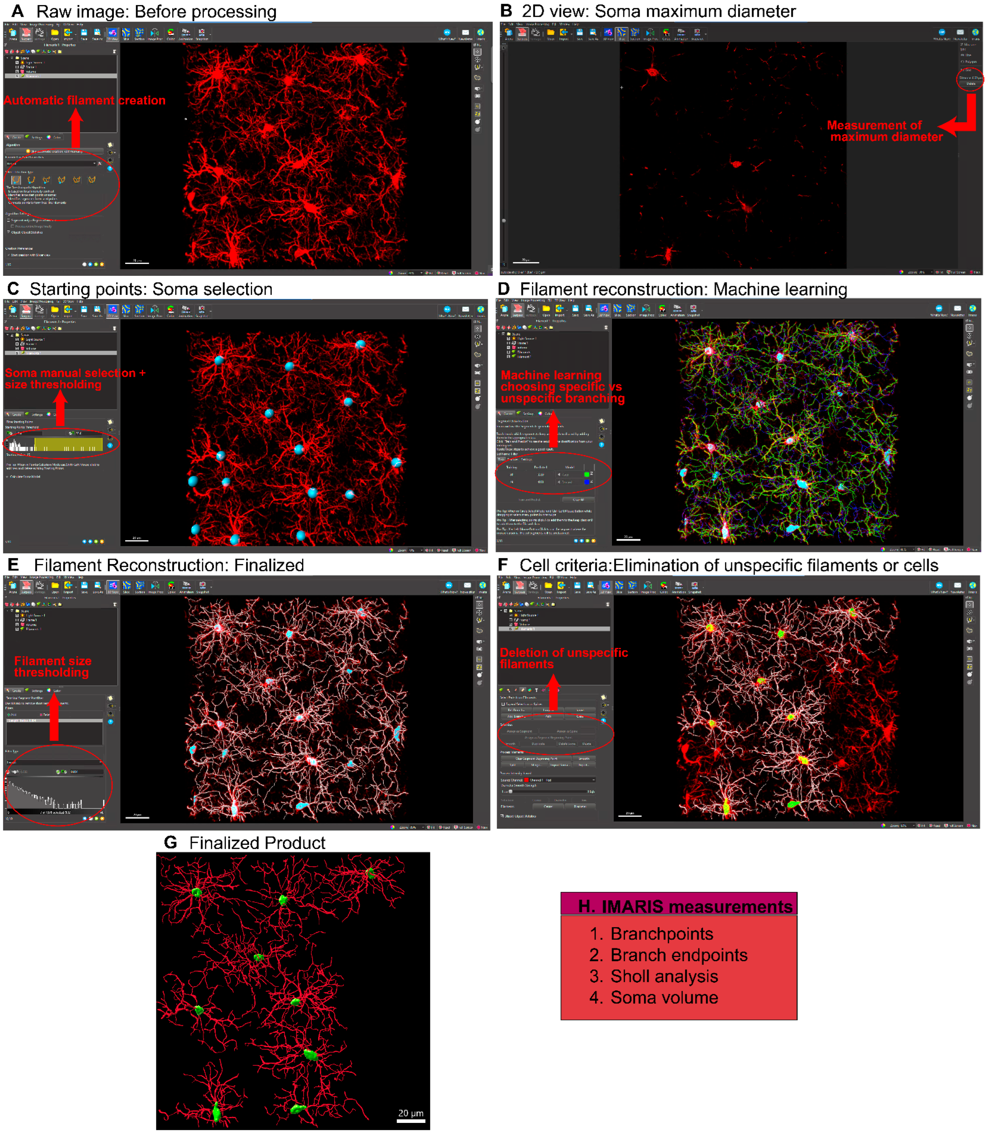
Figure 3.
Microglial Analysis Workflow Using CellSelect-3D Morph. A) Raw confocal image of microglia stained with IBA-1. B) The first step is to apply the Otsu thresholding technique, adjust the fluorescent intensity for reconstruction, and select a noise filter to reduce background signaling. C) Reconstructed image using the chosen Otsu threshold. D) At this stage, the entire image is reconstructed, and both the largest and smallest single cells are selected to filter out non-cellular structures and separate reconstructions where two cells are considered as one. E) 2D image showing the selected cells. F) This window allows for the selection of cells to be measured, filtering for incomplete cells. G) Reconstructed single-cell images (circled cell) outputted by the software. Panels 1-4 show different reconstructions representing the various parameters and measurements provided by the software.
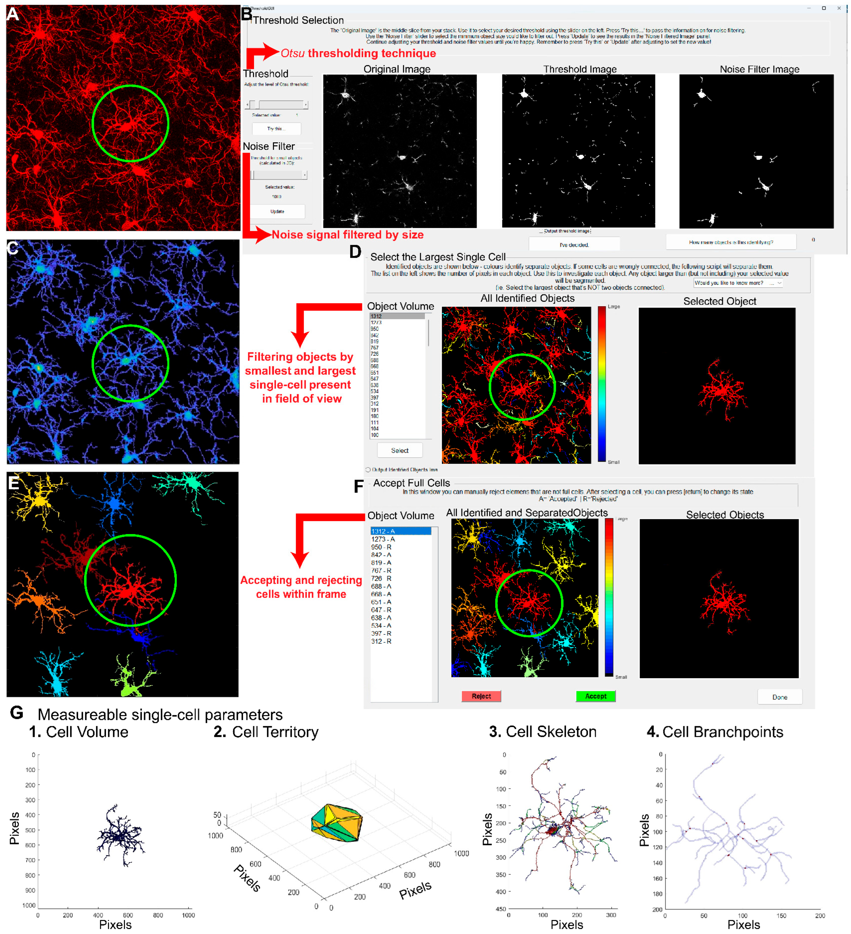
Figure 4.
Comparative Analysis of the Same Dataset Using CellSelect-3D Morph and IMARIS Software. The dataset was collected from naïve females rats treated with either vehicle (saline) or ATP disodium salt (50 mg/kg) 2 hours before perfusion and tissue collection. Comparable data were obtained from both software programs used. A) Timeline detailing the treatment with vehicle and ATP i.p. injections in naïve rats, followed by the perfusion protocol. B) Left panel: Raw images from confocal microscope of microglia stained with IBA-1 in vehicle and ATP-treated rats. Middle panel: Reconstruction of microglia using IMARIS software. Right panel: Reconstruction of microglia using CellSelect-3D Morph software. Figures C-F display parameters obtained using IMARIS software. Specifically, after ATP treatment panel C) shows a reduced number of intersections (95 % Confidence interval: [0.1970, 1.734]), D) depicts reduced the total number of filament branch points (r effect size=-0.1605, 95% Confidence interval median difference(CImd): [-41.00,-12.00]), and E) illustrates reduced the total number of filament endpoints(r =-0.1622, 95% CImd: [-21.00,-6.000]). Panel F) shows a reduction in cell body volume after ATP treatment (r =-0.4791, 95% CImd:[ -35.00,-18.00]),. Figures G-N display parameters obtained using CellSelect-3D Morph software. Specifically, after ATP treatment panel G) shows reduced cell territory (r =-0.1469, 95% CImd: [-7343,-680.8 ]), H) reduced cell volume(r =-0.2110, 95% CImd:[-166.1, -44.82]), I) reduced number of branchpoints (r =-0.1982, 95% CImd:[ -3.000, 0.000]), and J) number of endpoints (r =-0.1657, 95% CImd:[ -4.000,-1.000]),. Panel K-– N show no changes in ramification index, average branch length, and min and max branch length. Data are shown as median and quartiles. Fig C was analyzed with Mixed-effect analysis indicating a *p<0.0001 difference between ATP and Veh. Fig D-N were analyzed with non-parametric test Mann-Whitney indicating *p<0.05 difference between ATP and Veh, **p<0.01 difference between ATP and Veh, and ***p<0.001 difference between ATP and Veh. Fig D, F and G show the number of microglia/number of rats. Additional analysis was done with non-parametric test Kolmogorov-Smirnov on Fig D-N indicating * and** p<0.01 difference between ATP and Veh, and ***p<0.001 difference between ATP and Veh (Kolmogorov-Smirnov test showed no difference on panel J). Panel A was done using BioRender.com.
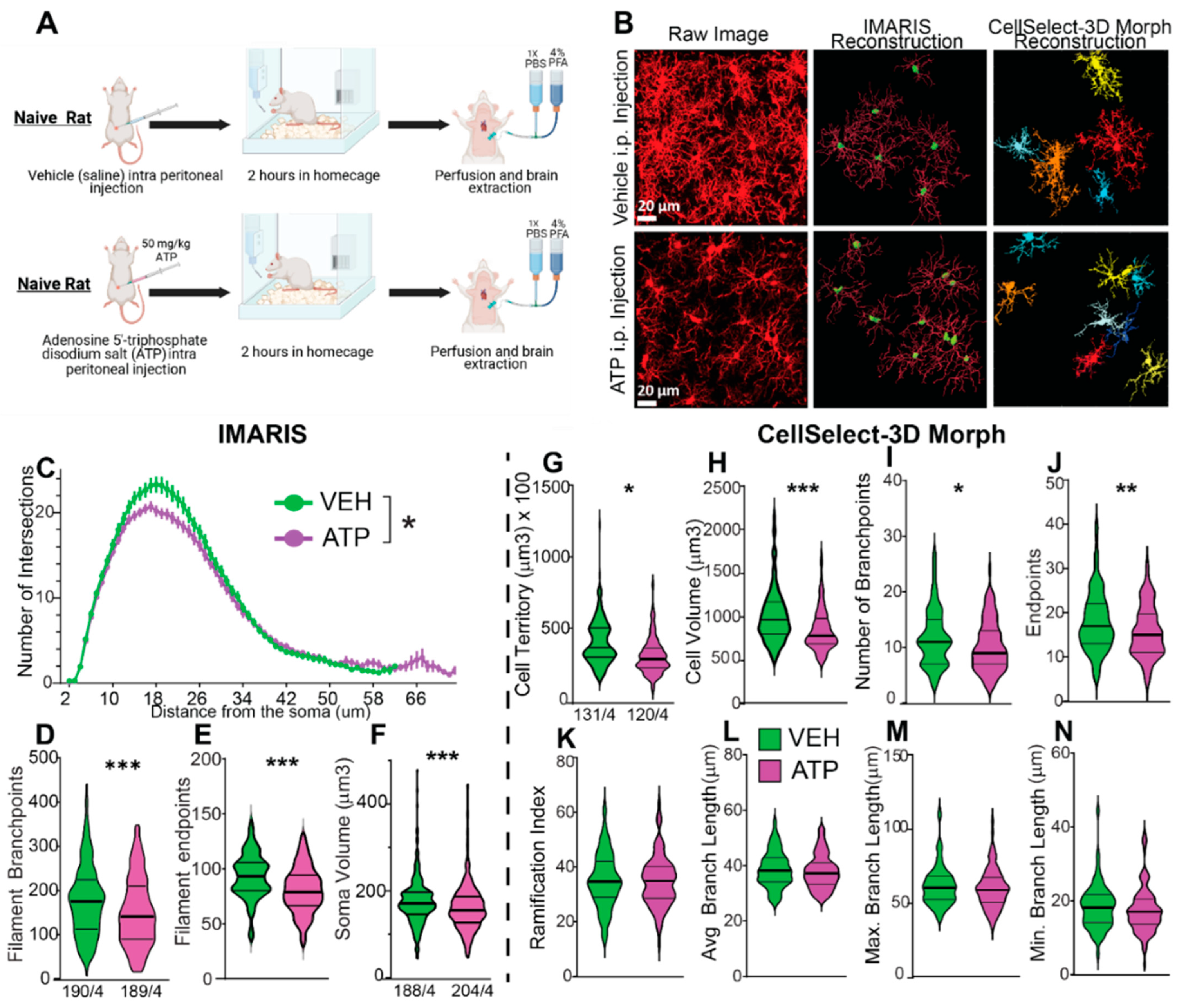
Figure 5.
Identification of Morphological Subpopulations Using CellSelect-3DMorph Clustering. This analysis approach provides deeper insights into microglial morphological diversity. A) Principal component analysis (PCA) loading matrix displaying all eight morphological parameters from CellSelect-3DMorph, with corresponding loading values per principal component. B) Variance explained by each PCA component, showing that the first two components account for 71.51% of the total variance. C) Cluster distribution across experimental groups, demonstrating that ATP treatment did not significantly alter microglial morphological distribution compared to VEH (p). D–F) Comparison of specific morphological features: cell territory (F(5,245)=8.783, p<0.0001), cell volume (F(5,245)=4.664, p<0.0001), and ramification index (F(5,245)=2.389, p<0.0001), between clusters and experimental conditions. Data is shown in quartiles and medians. Panel D-F) were analyzed using ordinary one way-ANOVA indicating differences between clusters within ATP and VEH groups, ****p<0.0001, as well as differences between cluster between ATP and VEH groups**p<0.01 and ***p<0.001. Panel C shows the number of the number of cells analyzed in each group/ animal, and the number of cells in each cluster.
Disclaimer/Publisher’s Note: The statements, opinions and data contained in all publications are solely those of the individual author(s) and contributor(s) and not of MDPI and/or the editor(s). MDPI and/or the editor(s) disclaim responsibility for any injury to people or property resulting from any ideas, methods, instructions or products referred to in the content. |
© 2025 by the authors. Licensee MDPI, Basel, Switzerland. This article is an open access article distributed under the terms and conditions of the Creative Commons Attribution (CC BY) license (http://creativecommons.org/licenses/by/4.0/).
Copyright: This open access article is published under a Creative Commons CC BY 4.0 license, which permit the free download, distribution, and reuse, provided that the author and preprint are cited in any reuse.


