
Submitted:
17 July 2025
Posted:
17 July 2025
You are already at the latest version
Abstract
Financial time series prediction remains a significant challenge, driven by market volatility, nonlinear dynamic characteristics, and the complex interplay between quantitative indicators and investor sentiment. Traditional time series models (e.g., ARIMA, GARCH) struggle to capture the nuanced sentiment in textual data, while static deep learning integration methods fail to adapt to market regime transitions (bull markets, bear markets, consolidation). This study proposes a hybrid framework that integrates investor forum sentiment analysis with adaptive deep reinforcement learning (DRL) for dynamic model integration. By constructing a domain-specific financial sentiment dictionary (containing 16,673 entries) based on sentiment analysis approach and word embedding technique, we achieve 97.35% accuracy in forum title classification tasks. Historical price data and investor forum sentimental information are then fed into three Transformer variants (single-layer, multi-layer, bidirectional) and a support vector regressor (SVR) for predictions, with a Deep Q-Network (DQN) agent dynamically fusing the prediction results. Comprehensive experiments are conducted on diverse financial datasets, including China Unicom, CSI 100 Index, corn, and Amazon (AMZN). Experimental results demonstrate that our proposed approach, combining textual sentiment with adaptive DRL integration, significantly enhances prediction robustness in volatile markets, achieving the lowest RMSEs across diverse commodities. It overcomes the limitations of static methods and achieves cross-commodity generalization, outperforming both benchmark and state-of-the-art models.
Keywords:
sentiment analysis
; transformer
; reinforcement learning
; market price prediction
; model ensembling
1. Introduction
Accurate forecasting of financial time series remains a cornerstone of global financial stability, with trillions of dollars in derivatives trading hinging on reliable predictions [1]. However, financial forecasting is inherently complex. Financial markets are inherently volatile, exhibiting unpredictable swings driven by a complex interplay of economic indicators, geopolitical events, and investor sentiment. (e.g., 20% daily swings in energy futures during geopolitical crises). These fluctuations are often amplified during periods of crisis, leading to significant uncertainty and risk. Moreover, the dynamics of financial markets are non-linear, shifting between periods of growth (bull markets) and decline (bear markets), making it difficult to develop models that consistently perform well across different regimes. The integration of both quantitative data (e.g., price, volume) and qualitative information (e.g., news sentiment, social media trends) is crucial but remains a significant challenge for many forecasting methods [2]. Yet, traditional time-series models like ARIMA [3] and GARCH [4] struggle to reconcile these complexities. During the 2020 COVID-19 crash, ARIMA underperformed deep learning by 42% in volatility prediction [5], while GARCH fails to adapt to volatility regime shifts during bear markets, exhibiting significantly higher prediction errors than decomposition-integration models in futures markets [6], highlighting their limitations in dynamic environments.
Recent advances in natural language processing (NLP) and deep learning have enabled sentiment integration. Li et al. [7] used Long Short-Term Memory (LSTM) with attention to Twitter sentiment for crude oil, achieving 78% trend accuracy but requiring commodity-specific feature engineering. Xu and Cohen [8] proposed a deep generative model combining tweet sentiment and price signals, introducing recurrent latent variables to handle market stochasticity. However, their approach requires dataset-specific feature engineering and lacks cross-commodity adaptability. Chen et al. [9] developed a graph convolutional feature based convolutional neural network (GC-CNN) to capture inter-stock correlations, improving trend prediction for Chinese equities, but its static graph structure fails to adapt to real-time regime transitions.
On the other hand, hybrid models show promise but remain constrained. Kabir et al. [10] combined LSTM, modified Transformer [11], and multilayer perceptron (MLP), reducing RMSE by 15% for stock indices. But using static models led to 30% higher errors during policy-driven crashes. Li et al. [7] proposed a secondary decomposition method for crude oil, which required 40% more training data, limiting scalability. Tsantekidis et al. [12] used diversity-driven distillation for reinforcement learning (RL) trading while 10+ million pre-trained samples were required, which is impractical for real-time market prediction.
In this paper, we address the above limitations by integrating a domain-specific sentiment dictionary, heterogeneous Transformer variants, and DQN-driven dynamic ensembling, enabling robust predictions across different kinds of commodities and market regimes.
2. Literature Review
2.1. Traditional Time Series Models and Deep Learning Baselines
Traditional time series models form the foundation of financial forecasting but exhibit critical limitations. Box and Jenkins’ ARIMA model [3] assumes linear relationships and stationary processes, proving inadequate for nonlinear market dynamics. During extreme events, such as the 2020 market crash, ARIMA underperformed deep learning models by 42% in volatility prediction [5], highlighting its inability to capture abrupt changes.
Bollerslev’s GARCH model [4] advanced volatility modeling via conditional heteroskedasticity, but its reliance on stationary regimes is problematic. Wang et al. [6] observed higher prediction errors when transitioning from bull to bear markets, evidencing its failure to adapt to regime shifts. These limitations have driven the adoption of deep learning baselines, such as [13,14]. For instance, Li et al. [15] proposed a Transformer-based framework for structural response prediction, demonstrating the potential of self-attention mechanisms in time-series modeling-an approach later adapted to financial forecasting contexts.
Wang et al. [13] evaluated SVR, LSTM [16], and gated recurrent unit (GRU) [17] for stock price prediction, finding that LSTM outperforms traditional models but still struggles with high volatility. Connor et al. [18] pioneered RNNs for robust time series prediction, while Graves and Schmidhuber [19] introduced bidirectional LSTM (BiLSTM) for framewise phoneme classification, later adapted for stock prediction [20]. Nelson et al. [21] used LSTM for stock market movement prediction, achieving moderate accuracy. Chen et al. [9] proposed a GC-CNN model to capture inter-stock correlations, outperforming traditional CNNs for Chinese equities. Yet, the use of single models may not fully capture the complexities of financial markets, prompting research into more advanced modeling strategies.
2.2. Single Models with Decomposition Methods or Advanced Techniques
Several deep learning models combines with decomposition methods or advanced techniques to further improve the learning ability. Wang et al. [16] proposed FIVMD-LSTM model, which integrates empirical mode decomposition (EMD) to predict CSI 100 [16]. Similarly, Mahmoodzadeh et al. [17] used grey wolf optimizer-LSTM (GWO-LSTM) for tunnel boring machine penetration rate forecasting, demonstrating improved stability, but with a relatively high RMSE on financial data. Lin et al. [5] integrated CEEMDAN with LSTM for volatility forecasting, achieving a relatively small mean absolute error (MAE) on CSI 100 [5], despite that their model requires extensive data decomposition, which limits the scalability. Li et al. [2] proposed an SSA-BIGRU model for time-series production forecasting, combining sparrow search algorithm with bidirectional GRU, but its high MAPE on financial data [2] highlights the challenge of capturing nonlinear dependencies. Zhang et al. [22] developed a VMD-SE-GRU model for oil price forecasting, integrating variational mode decomposition with squeeze-and-excitation GRU, yet high RMSE was obtained. However, the potential for improved forecasting accuracy remains due to the use of single model, motivating the development of more advanced approaches such as hybrid model approaches or adaptive strategy approaches.
2.3. Hybrid Models
Hybrid CNN-LSTM models have been proposed to leverage the strengths of both Convolutional Neural Networks (CNNs) and LSTMs for efficient feature extraction within time series data. Chen et al. [23] developed CNN-BiLSTM-ECA models, incorporating bidirectional LSTMs (BiLSTMs) to process information from both past and future time steps and integrating an efficient channel attention (ECA) mechanism to enhance the model’s ability to focus on the most relevant features. Kabir et al. [10] proposed an LSTM-mTrans-MLP hybrid model, reducing RMSE for stock indices, but static models lead to suboptimal performance during market crashes due to the use of fixed weights after training even the models are hybrid. These models demonstrate a lack of robustness in the face of extreme market events, suggesting a need for more resilient approaches.
2.4. Sentiment Analysis
Sentiment analysis has emerged as a critical component of financial forecasting, though challenges remain. Tetlock [1] proved that media sentiment significantly impacts stock markets, while Loughran and McDonald [24] developed a financial lexicon to address domain-specific nuances. Xu and Cohen [8] proposed a deep generative model for stock movement prediction from tweets, introducing recurrent latent variables, but their approach requires task-specific preprocessing and lacks cross-commodity generalization.
For cross-market forecasting, traditional methods often struggle with domain shift. Umer et al. [25] compared machine learning algorithms for stock market prediction, finding linear regression inadequate for volatile data. Omoware et al. [26] used LSTM for Amazon and Google stock prediction, obtained a large MAE. It is found that even though Google and Amazon are both in the tech industry sector, their individual business models, competitive landscapes, and risk profiles create unique sensitivities to various events, leading to potentially dissimilar stock price movements. Incorporating sentiment analysis enhances financial forecasting models by capturing company-specific factors, thereby improving their adaptability and accuracy across diverse stocks and markets.
2.5. Limitations of Existing Research and Our Contributions
To summarize, existing studies reveal four critical gaps:
- Inability to adapt to different market regimes: Static ensembling approaches, such as [12], fails to adjust to varying market conditions, making them impractical for real-time financial forecasting.
To address these gaps, a domain-specific financial sentiment dictionary is constructed using SnowNLP for sentiment analysis in the financial domain. A Word2Vec embedding model is employed for dictionary expansion. This dictionary is utilized to analyze sentimental information from investor forums, aiding in price forecasting across different market regimes and commodities, thereby overcoming the limitations of static models, even those using advanced techniques. The investor forum sentiment data is then combined with historical price data and fed into three Transformer variants (single-layer, multi-layer, and bidirectional) and a Support Vector Regressor (SVR) for predictions. A Deep Q-Network (DQN) agent dynamically fuses the prediction results across diverse market conditions and asset types. Therefore, our proposed framework has four core contributions:
- By making use of SnowNLP and Word2Vec, a domain-specific financial sentiment dictionary (16,673 entries) is proposed for investor forum sentiment analysis, which achieves 97.35% classification accuracy and surpasses generic lexicons in capturing market specialized terminology.
- In addition, a heterogeneous model framework is designed that integrates Support Vector Regression (SVR) for linear trend capture and three Transformer variants for nonlinear dependency modeling.
- Finally, comprehensive experiments are performed to validate the performance of our DQN-Hybrid Transformer-SVR Ensemble framework (DQN-HTS-EF) across a diverse portfolio of financial datasets, including Bitcoin, China United Network Communications (China Unicom), CSI 100 Index, Amazon (AMZN), and corn futures. This multi-asset design—encompassing RMB-denominated equities, USD-denominated tech stocks, cryptocurrency, and agricultural commodities—enables rigorous testing of cross-regime generalization.
3. Materials and Methods
3.1. Framework Overview
Our proposed hybrid framework architecture operates in three interconnected stages, leveraging sentiment semantics, multi-model heterogeneity, and deep reinforcement learning (DRL) adaptability, which is as shown in Figure 1.
- Domain-Specific Sentiment Dictionary Construction
With the proliferation of AI-generated financial texts (e.g., ChatGPT [28], QuillBot [29]), generic lexicons struggle to distinguish genuine investor sentiment from synthetic content [30]. A financial domain-specific dictionary is essential to capture nuanced financial specialized terminology and mitigate misclassification risks posed by AI-generated forum titles. The data acquisition and dictionary construction methods are detailed in Section 3.2 and Section 3.3 respectively.
Taking 400k financial research reports as the primary data source, the raw text is pre-processed, followed by sentiment scoring via SnowNLP [31], which results in a foundational dictionary containing 6,352 entries. The dictionary is then expanded using a financial-data-pretrained Word2Vec [30,32] (300-dimensional embeddings trained on financial corpora), yielding an expanded dictionary of 16,673 domain-specific terms.
- 2.
- Sentiment Feature Extraction for Forum Titles
The expanded dictionary constructed by Word2Vec is used to infer sentiment polarity of forum titles (a proxy for retail investor sentiment) with daily sentiment scores calculated. These sentiment scores are aggregated, then merged with historical time series market price data, forming a rich augmented feature set, i.e., historical price data with textual semantic scores, which is a critical input for our subsequent prediction models. This sentiment score calculation is mentioned in Section 3.4.
- 3.
- Dynamic Model Ensembling via DRL
The framework deploys four complementary prediction models for forecasting. A kernel-based Support Vector Regression (SVR) model [33] is used, which excels in capturing linear trends within stable markets by using an ϵ-insensitive tube to minimize prediction errors within a specified range. This SVR are complemented with three Transformer [10,34] architecture variants of modeling market trends with higher degree of complexity: the Base-Transformer (a single-layer encoder that leverages self-attention for sequential price-feature vector processing), the Multi-Transformer (a 3-layer stacked encoder, which captures long-range temporal dependencies in volatile markets), and the Bi-Transformer (a bidirectional encoder that processes both forward and reversed sequences to enhance contextual feature extraction from multi-directional market signals).
Instead of using static model ensembling approach, a more advanced deep Q-network (DQN) [35] is proposed to serve as the dynamic ensembler, treating the model predictions and trading volume as “states”, model selection as “actions”, and prediction error as “rewards” for deep reinforcement learning. This DQN adaptively weights the base model outputs in real-time to optimize cross-commodity forecasting. This design leverages model heterogeneity to balance linear trend capture (via SVR) and nonlinear dependency modeling (via Transformers), while DQN enables context-aware fusion tailored to evolving market conditions, optimizing for cross-commodity volatility. Finally, the predicted result output by DQN would be the final predicted market value. The whole hybrid model architecture plus DQN is mentioned in Section 3.5.
3.2. Data Acquisition and Data Preprocessing
In financial market prediction, the quality and diversity of data are the key foundations for building accurate models. This study comprehensively collected two types of crucial data, namely financial trading data and textual sentimental data, to fully capture market dynamics and investor sentiment.
3.2.1. Financial Trading Data
Four distinct financial trading data are extracted from diverse stock markets and countries to evaluate our advanced DQN-Hybrid Transformer-SVR Ensemble framework (DQN-HTS-EF). The datasets include stock price data of China United Network Communications Group Co., Ltd. (China Unicom, Beijing, China), the CSI 100 Index (one of the most researched RMB-denominated Chinese indices), Amazon (AMZN) stock prices (denominated in USD), and corn futures contracts traded on the Dalian Commodity Exchange (DCE). The China Unicom, CSI 100 Index, and corn futures datasets are derived from the Digquant Financial Database (https://digquant.com/) spanning January 1, 2020, to December 31, 2024, while the Amazon (AMZN) dataset is obtained from Yahoo Finance (https://finance.yahoo.com/) spanning May 25, 2017 to April 5, 2023. This multi-source dataset design enables cross-market validation, integrating RMB-denominated equities, USD-denominated tech stocks, and agricultural commodities for testing the model robustness.
3.2.2. Textual Sentimental Data
Web crawling was performed on the Eastmoney Stock Bar [36], which is a leading Chinese financial forum, to obtain textual sentimental data reflecting investor sentiment. Particularly, the forum title data related to the CSI 100 Index, DCE Corn, China Unicom, and AMZN, are scrapped. This can to leverage its rich source of investor sentiment expressed in forum titles After that, data preprocessing is performed. We first used regular expressions (regex) to remove special characters from the forum titles. For instance, a Chinese-to-English translated raw forum title like “Corn is going to skyrocket! #Futures Market @Investment Expert” would be transformed by regex to “Corn is going to skyrocket Futures Market Investment Expert” after removing the special characters “#”, “@”, and the exclamation mark “!”. Subsequently, stopwords were also eliminated, since stopwords are common words that typically carry little semantic meaning, such as “the”, “and”, “in” in English. If the title was “The price of Corn is rising”, after removing stopwords, it becomes “price Corn rising”. This step helps to reduce noise in the data and focuses more on the meaningful words related to sentiment and market views. After that, we employed the Jieba tokenizer [37], which is a Chinese word segmentation tool. For example, the sentence “The increase in demand causes the price of Corn to rise”, with also the preprocessing, would be eventually segmented into “increase”, “demand”, “causes”, “price”, “Corn,” “rise”. With our preprocessing and word tokenization, forum title is effectively split into individual words, which is essential for further sentiment analysis as it can accurately identify words in different contexts and enables us to extract sentiment-bearing words and phrases.
3.3. Financial Domain-Specific Sentiment Dictionary Construction
3.3.1. Dictionary Construction Using Sentiment Analysis
The construction of the financial domain-specific sentiment dictionary employed a rigorous two-stage methodology. Initially, 100 financial research reports spanning from May 24, 2023 to May 31, 2023 were manually annotated for sentiment polarity to establish a high-quality training corpus. By utilizing SnowNLP [13], each sentence was assigned a polarity score within the continuous range of [0, 1] where SnowNLP is used for sentiment analysis of a sentence in Chinese language. When the scores larger than or equal to 0.7 were classified as positive sentiment and those smaller than or equal to 0.3 were classified as negative sentiment. Among these sentences with either positive or negative sentiment, lexical items appearing with a minimum frequency of 3 in these categorized sentences were retained, which yields a foundational dictionary of 6,352 entries, reflecting the nuanced financial domain-specific sentiment expressions prevalent in financial research reports.
3.3.2. Dictionary Expansion Using Word Embedding
To further enhance the dictionary’s semantic coverage and domain relevance, an unsupervised learning expansion phase was implemented using the financial-data pre-trained 300-dimensional Word2Vec word embedding model, sgns.financial.word [38]. For each lexical entry in the initial dictionary, semantically proximate terms were identified by measuring the cosine similarity [39]. The cosine similarity between words and , , is calculated as follows:
where and denote the word vectors in the embedding space, represents the dot product of two word vectors. and are the L2 norms of the corresponding word vectors. When the cosine similarity is large, it means the semantic meanings of these two words are close to each other. Therefore, terms exhibiting cosine similarity larger than or equal to 0.8 to entries in the foundational dictionary were incorporated into the dictionary. Sentiment labels were assigned using majority voting among nearest neighbors. This process expanded the dictionary by 10,321 entries, culminating in a comprehensive financial sentiment dictionary of 16,673 terms.
3.4. Market and Sentiment Data Fusion for Model Prediction
Market data is typically described as quantitative because it consists of numerical values such as prices, volumes, and other measurable financial indicators while sentiment data is considered qualitative because it captures subjective information like opinions, emotions, or attitudes, often derived from text, social media, or news. The core input representation of our forecasting framework integrates quantitative market dynamics and qualitative sentiment signals, with the feature fusion process structured in Figure 2.
For quantitative data, the daily closing price and daily trading volume volatility are included as they are capturing the price trends and intensity of trading activity over time. the closing price at day t is min-max normalized to the range of [0, 1] as . And the trading volume volatility at day t is calculated using z-score standardization based on the k-day rolling mean and standard deviation as represented by , which formulated as below:
where , , and are the unnormalized trading volume, the mean value of k-day trading volume, and the standard deviation of k-day trading volume respectively, with k is set to 30 empirically.
For the qualitative data, an investor sentiment score is derived from Eastmoney forum titles [36]. Specifically, the investor sentiment score at day t, is scaled using a normalized difference between positive and negative word counts, which is formulated as below:
where and are respectively the positive and negative word counts across forum titles on day t. validated by our domain-specific financial dictionary as aforementioned in Section 3.3.
The above heterogeneous data features are then concatenated into a unified temporal input feature vector , preserving the causal alignment where (generated from forum titles at day t) is used to predict the price for the next day . To avoid look-ahead bias, the preprocessing protocol ensures temporal consistency by collecting forum titles at market close (15:00 CST) for the next-day market price prediction. A SHAP analysis [40] is performed to confirm that contributes to the prediction variance across commodities, which is described in Section 4.5.
3.5. The Proposed DQN-HTS-EF Model Architectures
In the rapidly evolving landscape of market price forecasting, single-model approaches often fall short in addressing the complexities and variabilities inherent in market behavior. To enhance prediction accuracy and adaptability, we propose an adaptive multi-model fusion strategy that leverages the strengths of various forecasting models. This approach allows for a more comprehensive analysis of diverse market conditions, improving the model’s ability to generalize across different scenarios. Specifically, four models are used for market price forecasting, which are Support Vector Regression (SVR), Base-Transformer, Multi-Transformer, and Bi-Transformer. Each model is chosen according to its unique strengths in handling different market conditions. SVR is adept at capturing trends in relatively smooth and volatile markets while the Transformer series excels in highly volatile environments with complex long- and short-term dependencies. By integrating these models, the overall generalization capability is enhanced across diverse market scenarios.
Furthermore, a deep reinforcement learning (DRL) model, Deep Q-Network (DQN) [35], is also integrated for selecting the best prediction from multiple models as mentioned above. With DQN, the prediction errors can be effectively reduced, and thereby achieves more accurate and reliable market price forecasting.
3.5.1. SVR Model for Smooth Market
While Support Vector Machine (SVM) is to find a hyperplane that maximizes the spacing from data points to the hyperplane in order to minimize the prediction error, SVR is the extension of SVM for solving the regression problem. In the context of financial market price forecasting, SVR is particularly effective for capturing trends in relatively smooth market conditions. Its core mechanism allows predicted values to fluctuate within a defined range known as the ϵ-insensitive tube, where loss is only incurred when the prediction error exceeds this threshold. SVR’s design, characterized by its ϵ-insensitive loss function that imposes no penalty on prediction errors within a predefined tolerance range (the ϵ-tube), inherently aligns with scenarios of less volatile price movements. In relatively smooth markets, where price fluctuations tend to be gradual and confined within narrow bounds, most prediction errors naturally fall within this ϵ-tube. By ignoring these minor deviations, SVR helps to avoid overfitting to transient noise and instead focuses on capturing the underlying trend, thus becoming adept at modeling the steady evolution of market prices in stable conditions.
Hence, SVR is used as one of our four models alongside Transformer-based approaches. It also serves as a baseline benchmarking model, allowing us to compare its performance in forecasting market prices. This comparison is essential for us to understand how different models respond to the complexities of the financial market, particularly in differentiating between stable and volatile market conditions.
3.5.2. Transformer Models for Moderate-to-Volatile Market
Transformer models [18] excel in managing long-distance dependencies within sequences, primarily due to their self-attention mechanism, which make them particularly renowned in natural language processing (NLP) and sequence modeling. This mechanism allows the model to process information at each position while simultaneously considering other relevant positions in the sequence, making them particularly suited for the complexities of market price forecasting.
In our market price prediction framework, we propose three Transformer models. The first one is the Base-Transformer model, which consists of a Transformer block followed by a fully connected layer. The last output of the last layer is used as our prediction. This architecture makes it ideal for scenarios where deep feature extraction is not necessary, e.g.,: moderate market. The second one is the Multi-Transformer, which is a multi-layer Transformer consisting a stack of multiple Transformer blocks, following by a fully connected layer. This setup allows for deeper feature extraction, enhancing model expressiveness and handling the volatile market. Last but not least, the third one is the Bi-Transformer, which is a bi-directional Transformer incorporating both forward and reverse Transformer blocks to process the original and flipped market sequences separately. This bi-directional information is then fused and output through a fully connected layer, aiming to comprehensively capture sequence context dependencies and increase the diverse perspective of the financial market data so as to improve prediction accuracy.
3.5.3. DQN for Adaptive Prediction Selection
Following the training of the four forecasting models, we implement a Deep Q-Network (DQN) [35] as a reinforcement learning mechanism to dynamically integrate their predictions where the states are the model predictions and trading volume the actions are the model selection, and the rewards are the prediction errors. Formally, the state vector at time step t is defined as:
where , , , and denotes the market price predictions of SVR, Base-Transformer, Multi-Transformer, and Bi-Transformer respectively. And is the normalized volume based on the k-day rolling mean and standard deviation as in (2).
The DQN processes to generate a Q-value vector of size 4, i.e., where represents the expected cumulative reward for selecting model at state . The final forecast, , is the market prediction of the model with the highest Q-value:
The network parameters are updated using the reward signal , where is the ground-truth market price data. The negative sign indicates that lower mean square error (MSE) results in a higher reward. This enables the DQN to refine its selection policy via temporal difference learning, adapting to evolving market regimes (e.g., stable vs. volatile) by prioritizing models that demonstrate consistent forecasting accuracy. In details, the network undergoes a training schedule consisting of 300 episodes, employing an ε-greedy exploration strategy (initial ε = 0.15, decay rate = 0.99) and Adam optimization (learning rate = 0.001) for policy refinement.
By integrating DQN with four models, our proposed framework is able to adapt to diverse market conditions. In stable markets, the agent preferentially utilizes the SVR model, leveraging its ability to capture smooth, gradual price trends. Conversely, in volatile markets, the DQN favors the Base-Transformer model, exploiting its capacity to model sentiment-driven, rapid price fluctuations. This adaptive model selection mechanism aligns with real-time market dynamics and eventually improves the forecasting performance.
4. Results
4.1. Dataset Information
Table 1 provides our dataset summary, encompassing start dates, end dates, total observations, and structured training-test splits.
Specifically, the CSI 100, Corn, and China Unicom datasets span from 2020-01-01 to 2024-12-31, with an 80:20 split yielding 969 training points and 243 testing points where the testing period (2024-01-02 to 2024-12-31) coinciding with the Russia-Ukraine war. This standardization ensures cross-comparability across heterogeneous financial commodities while preserving the temporal integrity of market signals for model construction.
For the AMZN dataset (2017-05-25 to 2023-04-05), the dataset employs a 70:30 split (1,034 training, 442 testing) covering the COVID-19 pandemic period (2021-07-06 to 2023-04-05). Each split adheres to chronological ordering to prevent look-ahead bias and information leakage, with testing periods deliberately spanning significant global events to validate model robustness under challenging conditions.
4.2. Performance Validation of Sentiment Scoring
4.2.1. Evaluation Metrics and Results
To assess the domain-specific financial sentiment dictionary, we employ standard classification metrics: Precision (P), Recall (R), and F1-score (F1). Precision is defined as the ratio of correctly classified semantic-positive (semantic-negative) instances to all predicted semantic-positive (semantic-negative) instances. Recall is measured as the ratio of correctly classified semantic-positive (semantic-negative) instances to all actual semantic-positive (semantic-negative) instances. And the F1-score is the harmonic mean of precision and recall, calculated as:
where and with TP, FP, and FN denoting the numbers of true positives, false positives, and false negatives, respectively.
On a holdout validation dataset of 50,000 forum titles, our extended dictionary achieved 97.35% validation accuracy, with F1-score of 0.94 (semantic-positive class) and 0.91 (semantic-negative class). With such high accuracy and F1-score, we are confident in the dictionary’s ability to be effectively deployed for our subsequent sentiment scoring and multi-model fusion prediction.
4.2.2. Sentiment Scoring Comparison and Examples
We also evaluated our Word2Vec-expanded dictionary by on 400K preprocessed forum titles. Among 16,673 terms in the dictionary, 14,849 terms were captured in 400K preprocessed forum titles, which is about 89% coverage, while generic lexicon HowNet [41] can only obtain about lower coverage of about 62%. This result reflects its efficacy in financial domain-specific terminology.
Some forum title examples are shown for illustration. For instance, semantic-positive titles like “CSI 100 surges 2% on policy stimulus, bullish signals persist” are correctly categorized via wordings like “surges” and “bullish”, while semantic-negative titles such as “Corn prices drop to 6-month low amid oversupply concerns” are identified through terms like “drop” and “oversupply”. These examples showcase the superior capability of our dictionary in capturing contextually relevant financial sentiment, underscoring its precision in identifying investor sentiment via industry-specific terminology.
4.2.3. Cross-Commodity Validation
Table 2 validates the generalizability of the domain-specific financial sentiment dictionary across four kinds of financial market data, demonstrating its robust performance in capturing nuanced sentiment across diverse commodity classes and market regimes. In the high-volatility CSI 100 Index dataset (92,184 forum titles), the dictionary achieves 97.00% classification accuracy, correctly labeling 52.57% (48,459) of titles as positive (e.g., policy-driven rally signals) and 9.52% (8,774) as negative (e.g., crash warnings), and the remaining 37.91% (34,951) as neutral. This highlights its effectiveness in discerning sentiment amid extreme market fluctuations.
For the relatively stable corn market (135,110 titles), the accuracy reaches 97.35%, with 42.23% (57,055) positive, 15.75% (21,285) negative, and 42.02% (56,770) neutral labels, showcasing its reliability in capturing sentiment under low-volatility conditions.
Similarly, the China Unicom dataset (153,023 titles) yields a 97.16% accuracy, classifying 53.91% (82,491) as positive and 11.12% (16,857) as negative, and 34.97% (53,675) as neutral, demonstrating its adaptability to corporate stock sentiment analysis.
Notably, the Amazon (AMZN) dataset (7,382 titles) achieves 90.53% accuracy, with 77.43% (5,716) positive and 6.18% (456) negative, and 16.39% (1,210) neutral labels, reflecting its cross-market applicability despite smaller sample size and USD-denominated market context. Collectively, these results validate the dictionary’s ability to generalize across commodities (equities, indices, agricultural futures).
4.2.4. Regression Analysis of the Sentiment Score - Closing Price Relationship
Table 3 presents the regression analysis across multiple datasets. Regression analysis is a statistical technique used to model the relationship between a dependent variable and one or more independent variables. Here, it details the regression coefficients for both the constant term and the sentiment score, along with their corresponding t-values.
In financial markets, investor sentiment is widely recognized as a key determinant of asset prices. Our study employed linear regression on datasets from AMZN, China Unicom, stock index, and corn to explore the relationship between sentiment score and closing price. The variation in regression coefficients among datasets is notable.
For AMZN dataset, the regression coefficient for the constant is 98.443 and for the sentiment score is 26.526, with t-values of 59.057 and 9.910 respectively. Positive correlations between sentiment score and closing price were observed in the AMZN. This suggests that in these markets, as the sentiment score (reflecting investor sentiment) increases, the closing price of the assets also tends to rise.
In contrast, for the China Unicom Data with sentiment Score, the regression coefficient for the sentiment score is -0.488, indicating an inverse relationship, and its t-value is -2.450. Similarly, the regression coefficient for the sentiment score is -327.564 for corn, with t-value being -4.703. Negative correlations emerged in the China Unicom means that an increase in the sentiment score is associated with a decrease in the closing price, potentially due to the unique market dynamics, investor expectations, or product-specific factors of these financial products.
Regarding significance, the sentiment score had a significant impact on closing prices in AMZN, China Unicom, and corn since the absolute t-values were large enough in these cases, which validates the influence of investor sentiment on financial product prices. However, in the CSI 100 stock index data, the sentiment score had an insignificant impact as indicated by its low t-value of 0.105. This implies that in the stock index market, macro-level factors such as overall economic trends, monetary policies, and geopolitical events play a dominant role in price formation, overshadowing the effect of investor sentiment.
4.3. Model Performance and Comparison
4.3.1. Evaluation Metrics
To comprehensively validate the effectiveness and generalization capability of the proposed framework, this study adopts the standard evaluation paradigm in the field of financial time series forecasting: by comparing the framework with traditional statistical methods, mainstream deep learning models, and the latest state-of-the-art (SOTA) approaches across diverse datasets (encompassing stocks, indices, agricultural futures, and Amazon (AMZN) stock), and quantifying errors using multi-dimensional metrics including Mean Squared Error (MSE), Root Mean Squared Error (RMSE), Mean Absolute Error (MAE), and Mean Absolute Percentage Error (MAPE). Four key examined metrics are presented as follows:
where , , and N are the ground-truth real market price, predicted market price, and the number of samples, respectively. Comprehensive experiments are conducted to evaluate the model performance and robustness across diverse financial commodities in order for model comparison under different volatility and complexity levels, highlighting strengths and limitations of different approaches, with particular focus on stable versus erratic futures market behaviors.
4.3.2. Performance Evaluation on CSI 100 Index
Table 4 presents the comparison of our proposed DQN-HTS-EF performance with the latest state-of-the-art (SOTA) approaches and traditional deep learning models on the CSI 100 index dataset using the MAPE, RMSE, and MAE metrics.
Compared to other benchmarking models [2,5,13,14,22], our proposed DQN-HTS-EF achieves superior results with the lowest MAPE of 2.027, RMSE of 148.7959, and MAE of 106.9365. This demonstrates that our proposed framework enhances prediction accuracy for financial forecasting by integrating multi-model fusion with deep reinforcement learning via DQN.
4.3.3. Performance Evaluation on Corn Futures
Table 5 presents the comparison of our proposed DQN-HTS-EF performance with the latest SOTA approaches and traditional deep learning models on the corn futures dataset. Similarly, our proposed DQN-HTS-EF achieves superior with the lowest MAPE of 1.075, RMSE of 30.835, and MAE of 24.826, which significantly outperforms other benchmarking models [6]. This result demonstrates our proposed framework improves the prediction accuracy for agricultural commodity time series forecasting.
4.3.4. Performance Evaluation on China Unicom Stock
Moreover, Table 6 tabulates the performance evaluation of our DQN-HTS-EF on the China Unicom stock dataset. As we can see, compared to the existing approaches [9,10,18,19,23] including the hybrid model LSTM-mTrans-MLP [10], our DQN-HTS-EF outperformed them with the lowest MSE of 0.012, RMSE of 0.108, and MAE of 0.075. Notably, it outperforms static hybrid models (e.g., LSTM-mTrans-MLP [10]) by 33.3% in MSE for China Unicom dataset, establishing a new benchmark for adaptive financial forecasting. This again suggests that our model significantly improves prediction accuracy.
4.3.5. Performance Evaluation on Amazon Stock
Last but not least, Table 7 presents the performance comparison of our DQN-HTS-EF with the latest SOTA approaches on the Amazon stock dataset. Our DQN-HTS-EF outperformed the existing approaches [8,23,25,26] including the hybrid model CNN+BiLSTM [23] with the lowest MAE of 4.335, RMSE of 5.293, and MSE of 28.018, which proves that our model supremacy.
To summarize, across all datasets, our DQN-HTS-EF consistently reduce the prediction errors by 12.9–48.5% against SOTA approaches, attributed to its dynamic ensemble strategy. The DQN agent’s real-time volatility adaptation—via a reward function tied to MSE— optimally balances the linear trend modeling of SVR with the nonlinear dependency capture of Transformers. Furthermore, the framework’s cross-commodity generalizability—from RMB-denominated indices to USD-tech stocks—highlights its potential for real-world financial applications.
4.4. Forecasting Performance Across Time
The predictions across time for four commodities are visualized in Figure 3, Figure 4, Figure 5 and Figure 6 to verify the adaptability advantage of DQN-HTS-EF in different market structures, each of which reflects different commodity dynamics and integrated customized responses.
4.4.1. Prediction Across Time on CSI 100 Index
For the CSI 100 Index (Figure 3), a volatility-dominated equity market sensitive to policy shifts and sentiment shocks (e.g., the 2024–10 rally), our DQN-HTS-EF (purple) tightly tracks the actual price (black). To capture abrupt sentiment-driven fluctuations, the usage of models is also counted. It is found that our DQN agent dynamically increases the usage of the Base-Transformer (blue) to 42% of predictions, leveraging its attention mechanism. In contrast, SVR as reported in [13], over-smooths extreme volatility with a higher RMSE of 469.6172. Meanwhile, FIVMD-LSTM [13] exhibits greater bias with an RMSE of 154.6032, compared to our model’s RMSE of 148.7959 as shown in Table 4—highlighting the ensemble’s superior balance between stability and responsiveness.
4.4.2. Prediction Across Time on Corn Futures
In the corn futures market (Figure 4), characterized by stable supply–demand dynamics and minor trend-adjacent fluctuations, our DQN-HTS-EF (purple) outperforms all single models. The ensemble prioritizes SVR (58% of predictions) for kernel-based smoothness to exploit linear trends, while Transformer insights (42% of predictions) are also integrated to refine local fluctuations. This dynamic multi-model fusion strategy using DQN minimizes bias, avoiding SVR’s underfitting on minor swings, and minimizes variance by mitigating Transformer from overfitting to noise, resulting in RMSE of 30.835—less than half of SVR’s 74.215 and 44.3% lower than SCINet [6] (Table 5), yielding the lowest MAPE of 1.075.
4.4.3. Prediction Across Time on China Unicom Stock
For China Unicom stock (Figure 5), it is a high-frequency tech stock which is sensitive to sector-specific news and sentiment spikes (e.g., late-2024 rallies). Our DQN-HTS-EF adapts by allocating 42% of predictions to Transformers for sentiment-driven pattern capture while using SVR for regularization to avoid overfitting. This balance is reflected in quantitative metrics with MAE of 0.075 achieved, which is a 4.7% reduction against the MAE of 0.110 by CNN-BiLSTM [23] (Table 6), demonstrating efficiency in tracking high-frequency fluctuations.
4.4.4. Prediction Across Time on Amazon Stock
For Amazon’s stock (Figure 6), it exhibits multi-year cycles and regime shifts (e.g., the 2022 downturn and 2023 recovery), which can validate the cross-regime adaptability of our DQN-HTS-EF. During the 2022 bear market, our DQN-HTS-EF increases the usage on the Multi-Transformer (green, 38% of predictions) to capture long-term trend reversals. During the 2023 recovery, it prioritizes the Single Transformer (45% of predictions) for short-term momentum. This dynamic selection yields an RMSE of 5.293, outperforming 5.336 by CNN-BiLSTM [23] and also other traditional models (Table 7). This underscores the generalizability of our proposed approach across complex market structures.
4.4.5. Statistical Validation
Statistical validation via paired t-tests is also conducted. We confirmed that the ensemble’s improvements were highly significant (p < 0.001 for all assets), with lower variance across datasets—e.g., CSI 100’s MSE of 0.0024 versus Transformer’s 0.0090—reflecting its effective navigation of the bias–variance trade-off. By dynamically selecting the optimal model mix for each scenario, the DQN-HTS-EF reduces both bias (through context-specific model selection) and variance (by avoiding single-architecture overreliance). These findings demonstrate the framework’s versatility in leveraging SVR for trend stability and Transformer variants for volatility modeling, establishing it as a robust solution for predictive tasks across heterogeneous financial assets.
Collectively, the visualizations (Figure 3, Figure 4, Figure 5 and Figure 6) confirm our DQN-HTS-EF’s ability to navigate the bias–variance trade-off: leveraging Transformer variants for pattern recognition in volatile/high-frequency contexts, prioritizing SVR for stability in trend-dominated markets, and dynamically adapting across multi-regime assets. Statistical validation (paired t-test, p < 0.001) and quantitative comparisons (Table 4, Table 5, Table 6 and Table 7) further solidify its superiority across heterogeneous commodities.
4.5. Further Analysis
4.5.1. SHAP Analysis Sentiment Scores and Model Predictions
To evaluate the contribution of sentiment scores , as in (3), SHAP analysis [40] is performed across different datasets. Table 8 shows the SHAP importance of , the ratio of positive to negative impacts, the dominant predictive model(s) for each dataset, and the SHAP importance of those dominant models. Corn Futures shows the lowest impact (0.003), suggesting sentiment plays a minimal role in predicting its price movements. In contrast, AMZN Stock exhibits a substantially higher SHAP importance (0.0367), indicating a much stronger influence of sentiment on its price prediction.
The dominant predictive models also differ across datasets. This suggests that the optimal predictive model may be asset-specific, reflecting the unique characteristics of each commodity.
This SHAP analysis demonstrates that sentiment plays a significant role in predicting the price movements. Furthermore, the choice of predictive model appears to be asset-specific, highlighting the need for DQN-based hybrid modeling.
4.5.2. Comparison with Alternative Ensemble Strategies
To further validate the effectiveness of our Proposed DQN-HTS-EF-driven dynamic ensembling strategy, we compare it against three conventional static ensemble methods: arithmetic mean (simple average of all model predictions), weighted average (weights determined by inverse MSE of individual models during training), and directional voting (predictions aligned with the majority direction of component models, converted to regression values via linear scaling).
Table 9 presents the MSE results of these strategies across the four financial datasets, highlighting the superiority of proposed DQN-HTS-EF’s adaptive weighting in handling market volatility and regime shifts. We can see that the proposed DQN-HTS-EF consistently achieves the lowest values across all datasets. For instance, in the CSI 100 Stock Index, its value is 0.0015, far lower than 0.0087, 0.0020, and 0.0140 by arithmetic mean, weighted average, and directional voting respectively. Similar advantages are also seen in Corn Futures, China Unicom Stock, and AMZN Stock.
5. Conclusions
In this paper, a hybrid framework is proposed, which integrates a domain-specific financial sentiment dictionary, heterogeneous Transformer variants, and a Deep Q-Network (DQN)-driven dynamic ensembling strategy to tackle the complexities of financial time series forecasting, including market volatility, nonlinear regime shifts, and the integration of quantitative indicators with investor sentiment. The framework constructs a 16,673-term sentiment dictionary using SnowNLP and Word2Vec, achieving 97.35% accuracy in classifying forum titles, which effectively captures financial domain-specific terminology. By combining Support Vector Regression (SVR) for linear trend modeling as well as three Transformer architectures (Base-Transformer, Multi-Transformer, Bi-Transformer) for nonlinear dependency extraction, the framework balances stability and adaptability. And our DQN is able to dynamically fuse model predictions based on real-time volatility, reducing RMSE by large margin on average across diverse datasets.
Comprehensive experiments are conducted across CSI 100 index, corn futures, China Unicom, and Amazon stock data, which demonstrates the framework’s superiority over state-of-the-art approaches. For instance, on CSI 100 index, it achieves the lowest MAPE of 2.027. In corn futures, it reduces RMSE to 30.835, a 44.3% improvement over SCINet (55.404). In high-frequency markets like China Unicom and Amazon, it surpasses CNN-BiLSTM baselines by 4.1% and 0.8% in MAE, respectively. This demonstrates cross-commodity generalization of our framework across RMB equities, USD tech stocks, and agricultural futures and validates its robustness during global events like the Russia-Ukraine war and COVID-19 pandemic.
The research advances financial forecasting by bridging sentiment analysis with adaptive model integration, showing that DRL-driven ensembling enhances prediction robustness. Practically, it offers a scalable solution for real-time markets, requiring minimal pre-training compared to static ensembles. The framework’s dynamic weighting of SVR and Transformers optimizes performance in both stable and volatile regimes.
Future work will focus on integrating event-driven features, exploring advanced RL algorithms like Proximal Policy Optimization (PPO) for handling rare black swan events which have limited historical data only, and extending to multi-time scale intraday forecasting. Overall, this research establishes a robust paradigm for sentiment-driven financial prediction, combining NLP, deep learning, and DRL to enable adaptive decision-making in dynamic markets.
Author Contributions
Conceptualization, Zhicong Song and Harris Sik-Ho Tsang; Data curation, Zhicong Song; Formal analysis, Zhicong Song and Harris Sik-Ho Tsang; Funding acquisition, Harris Sik-Ho Tsang and Wai-Lun Lo; Investigation, Zhicong Song and Harris Sik-Ho Tsang; Methodology, Zhicong Song, Harris Sik-Ho Tsang and Richard Tai-Chiu Hsung; Project administration, Harris Sik-Ho Tsang, Richard Tai-Chiu Hsung, Yulin Zhu and Wai-Lun Lo; Resources, Zhicong Song; Software, Zhicong Song; Supervision, Harris Sik-Ho Tsang and Richard Tai-Chiu Hsung; Validation, Zhicong Song and Harris Sik-Ho Tsang; Visualization, Zhicong Song; Writing – original draft, Zhicong Song, Harris Sik-Ho Tsang and Richard Tai-Chiu Hsung; Writing – review & editing, Harris Sik-Ho Tsang, Richard Tai-Chiu Hsung, Yulin Zhu and Wai-Lun Lo.
Funding
This research was funded by Hong Kong Chu Hai College.
Data Availability Statement
The data presented in this study are available on request from the corresponding author.
Conflicts of Interest
The authors declare no conflict of interest.
Abbreviations
The following abbreviations are used in this manuscript:
| AMZN | Amazon |
| ARIMA | Autoregressive Integrated Moving Average |
| BiLSTM | Bidirectional Long Short-Term Memory |
| BO | Bayesian Optimization |
| CEEMDAN | Complete Ensemble Empirical Mode Decomposition with Adaptive Noise |
| CNN | Convolutional Neural Network |
| CSI | China Securities Index |
| CST | China Standard Time |
| DRL | Deep Reinforcement Learning |
| DQN | Deep Q-Network |
| DQN-HTS-EF | DQN-Hybrid Transformer-SVR Ensemble framework |
| ECA | Efficient Channel Attention |
| FIVMD | Fast Iterative Variational Mode Decomposition |
| FN | False Negatives |
| FP | False Positives |
| GARCH | Generalized Autoregressive Conditional Heteroskedasticity |
| GC-CNN | Graph Convolutional Neural Network |
| GRU | Gated Recurrent Unit |
| GWO | Grey Wolf Optimizer |
| LSTM | Long Short-Term Memory |
| MA | Moving Average |
| MAE | Mean Absolute Error |
| MAPE | Mean Absolute Percentage Error |
| MDPI | Multidisciplinary Digital Publishing Institute |
| MLP | Multilayer Perceptron |
| MSE | Mean Square Error |
| NMSE | Negative Mean Squared Error |
| NLP | Natural Language Processing |
| PPO | Proximal Policy Optimization |
| regex | Regular Expression |
| RL | Reinforcement Learning |
| RMB | Renminbi Currency |
| RMSE | Root Mean Square Error |
| RNN | Recurrent Neural Network |
| SHAP | SHapley Additive exPlanations |
| SOTA | State-Of-The-Art |
| SSA-BIGRU | Sparrow Search Algorithm-Bidirectional Gated Recurrent Unit |
| SVM | Support Vector Machine |
| SVR | Support Vector Regression |
| TP | True Positives |
| USD | US Dollar |
| VMD-SE-GRU | Variational Mode Decomposition-Squeeze-and-Excitation Gated Recurrent Unit |
References
- Tetlock, P.C. Giving Content to Investor Sentiment: The Role of Media in Stock Markets. J. Finance 2007, 62, 1139–1168. [Google Scholar] [CrossRef]
- Lu, Y. Investor Sentiment and Stock Price Change: Evidence from CSI 500 Index. E-Commerce Lett. 2025, 14, 836–846. [Google Scholar] [CrossRef]
- Box, G.E.; Jenkins, G.M. Time Series Analysis: Forecasting and Control, 1st ed.; Holden-Day: San Francisco, CA, USA, 1970. [Google Scholar]
- Bollerslev, T. Generalized Autoregressive Conditional Heteroskedasticity. J. Econometrics 1986, 31, 307–327. [Google Scholar] [CrossRef]
- Lin, Y.; et al. Forecasting the Realized Volatility of Stock Price Index: A Hybrid Model Integrating CEEMDAN and LSTM. Expert Syst. Appl. 2022, 206, 117736. [Google Scholar] [CrossRef]
- Wang, Y.; et al. A Study of Futures Price Forecasting with a Focus on the Role of Different Economic Markets. Information 2024, 15, 817. [Google Scholar] [CrossRef]
- Li, J.; Zhang, H.; Wang, Y.; et al. A Novel Secondary Decomposition Method for Forecasting Crude Oil Price with Twitter Sentiment. Energy 2023, 268, 126345. [Google Scholar] [CrossRef]
- Xu, Y.; Cohen, S.B. Stock Movement Prediction from Tweets and Historical Prices. In Proceedings of the 56th Annual Meeting of the Association for Computational Linguistics (Volume 1: Long Papers), Melbourne, Australia, 15–20 July 2018; Association for Computational Linguistics: Stroudsburg, PA, USA, 2018; pp. 1970–1979. [Google Scholar]
- Chen, W.; Jiang, M.; Zhang, W.-G.; Chen, Z. A Novel Graph Convolutional Feature Based Convolutional Neural Network for Stock Trend Prediction. Inf. Sci. 2021, 556, 67–94. [Google Scholar] [CrossRef]
- Kabir, M.R.; Bhadra, D.; Ridoy, M.; Milanova, M. LSTM–Transformer-Based Robust Hybrid Deep Learning Model for Financial Time Series Forecasting. Sci 2025, 7, 7. [Google Scholar] [CrossRef]
- Vaswani, A.; Shazeer, N.; Parmar, N.; Uszkoreit, J.; Jones, L.; Gomez, A.N.; Kaiser, L.; Polosukhin, I. Attention Is All You Need. Advances in Neural Information Processing Systems 2017, 30, 5998–6008. [Google Scholar]
- Tsantekidis, A.; Li, Y.; Zhang, X.; et al. Diversity-Driven Knowledge Distillation for Financial Trading Using Deep Reinforcement Learning. Neural Networks 2021, 140, 249–263. [Google Scholar] [CrossRef] [PubMed]
- Wang, J.; Liu, J.; Jiang, W. An Enhanced Interval-Valued Decomposition Integration Model for Stock Price Prediction Based on Comprehensive Feature Extraction and Optimized Deep Learning. Expert Syst. Appl. 2023, 243, 122891. [Google Scholar] [CrossRef]
- Mahmoodzadeh, A.; Nejati, H.R.; Mohammadi, M.; Ibrahim, H.H.; Rashidi, S.; Rashid, T.A. Forecasting Tunnel Boring Machine Penetration Rate Using LSTM Deep Neural Network Optimized by Grey Wolf Optimization Algorithm. Expert Syst. Appl. 2022, 209, 118303. [Google Scholar] [CrossRef]
- Li, Z.Q.; Li, D.S.; Sun, T.S. A Transformer-Based Bridge Structural Response Prediction Framework. Sensors 2022, 22, 3100. Shen, B.; Yang, S.; Gao, X.; Li, S.; Ren, S.; Chen, H. A Novel CO₂-EOR Potential Evaluation Method Based on BO-LightGBM Algorithms Using Hybrid Feature Mining. SSRN Electron. J. 2022, 222, 211427. [CrossRef]
- Hochreiter, S.; Schmidhuber, J. Long Short-Term Memory. Neural Computation 1997, 9, 1735–1780. [Google Scholar] [CrossRef] [PubMed]
- Cho, K.; Van Merriënboer, B.; Gulcehre, C.; Bahdanau, D.; Bougares, F.; Schwenk, H.; Bengio, Y. Learning Phrase Representations Using RNN Encoder-Decoder for Statistical Machine Translation. arXiv 2014. [Google Scholar] [CrossRef]
- Connor, J.; Martin, R.; Atlas, L. Recurrent Neural Networks and Robust Time Series Prediction. IEEE Trans. Neural Netw. 1994, 5, 240–254. [Google Scholar] [CrossRef] [PubMed]
- Graves, A.; Schmidhuber, J. Framewise Phoneme Classification with Bidirectional LSTM and Other Neural Network Archi-tectures. Neural Netw. 2005, 18, 602–610. [Google Scholar] [CrossRef] [PubMed]
- Xu, Y.; Chhim, L.; Zheng, B.; Nojima, Y. Stacked Deep Learning Structure with Bidirectional Long-Short Term Memory for Stock Market Prediction. In Neural Computing for Advanced Applications, Kyoto, Japan, 12–14 October 2020; Springer: Cham, Switzerland, 2020; pp. 33–44. [Google Scholar]
- Nelson, D.M.Q.; Pereira, A.C.M.; de Oliveira, R.A. Stock Market’s Price Movement Prediction with LSTM Neural Net-works. In Proceedings of the 2017 International Joint Conference on Neural Networks (IJCNN), Anchorage, AK, USA, 14–19 May 2017; IEEE: New York, NY, USA, 2017; pp. 1419–1426. [Google Scholar]
- Zhang, S.; Luo, J.; Wang, S.; Liu, F. Oil Price Forecasting: A Hybrid GRU Neural Network Based on Decomposition–Reconstruction Methods. Expert Syst. Appl. 2023, 218, 119617. [Google Scholar] [CrossRef]
- Chen, Y.; Fang, R.; Liang, T.; Sha, Z.; Li, S.; Yi, Y.; Zhou, W.; Song, H. Stock Price Forecast Based on CNN-BiLSTM-ECA Model. Sci. Program. 2021, 2021, 2446543. [Google Scholar] [CrossRef]
- Loughran, T.; McDonald, B. When Is a Liability Not a Liability? J. Finance 2011, 66, 35–68. [Google Scholar] [CrossRef]
- Umer, M.; Awais, M.; Muzammul, M. Stock Market Prediction Using Machine Learning (ML) Algorithms. ADCAIJ Adv. Distrib. Comput. Artif. Intell. J. 2019, 8, 97–116. [Google Scholar] [CrossRef]
- Omoware, J.M.; Abiodun, O.J.; Wreford, A.I. Predicting Stock Series of Amazon and Google Using Long Short-Term Memory (LSTM). Asian Res. J. Curr. Sci. 2023, 5, 205–217. [Google Scholar]
- Mnih, V.; Kavukcuoglu, K.; Silver, D.; et al. Human-Level Control through Deep Reinforcement Learning. Nature 2015, 518, 529–533. [Google Scholar] [CrossRef] [PubMed]
- Brown T; et al. Language Models are Few-shot Learners, Advances in Neural Information Processing Systems, Virtual Conference, Dec. 2020, Vol. 33, pp. 1877-1901.
- Fitria, T.N. QuillBot as an online tool: Students’ alternative in paraphrasing and rewriting of English writing Englisia. J. Lang. Educ. Humanit. 2021, 9, 183–196. [Google Scholar] [CrossRef]
- Arshed, M.A.; Gherghina, Ș.C.; Dur-E-Zahra; Manzoor, M. Prediction of Machine-Generated Financial Tweets Using Ad-vanced Bidirectional Encoder Representations from Transformers. Electronics 2024, 13, 2222. [Google Scholar] [CrossRef]
- Sun, F.; Belatreche, A.; Coleman, S.; McGinnity, T.M. Pre-Processing Online Financial Text for Sentiment Classification: A Natural Language Processing Approach. In IEEE Computational Intelligence for Financial Engineering and Economics 2014, London, UK, 21–23 April 2014; IEEE: New York, NY, USA, 2014. [Google Scholar] [CrossRef]
- Mikolov, T.; Chen, K.; Corrado, G.; Dean, J. Efficient Estimation of Word Representations in Vector Space. International Con-ference on Learning Representations, Scottsdale, Arizona, USA, May 2013, pp. 1–12.
- Yan, R.; Jin, J.; Han, K. Reinforcement Learning for Deep Portfolio Optimization. Electronic Research Archive 2024, 32, 5176–5200. [Google Scholar] [CrossRef]
- Nayak, G.H.H.; Patra, M.R.; Swain, R.K. Transformer-Based Deep Learning Architecture for Time Series Forecasting. Softw. Impacts 2024, 22, 100716. [Google Scholar] [CrossRef]
- Mnih, V.; Kavukcuoglu, K.; Silver, D.; Graves, A.; Antonoglou, I.; Wierstra, D.; Riedmiller, M. Playing Atari with Deep Rein-forcement Learning, Neural Information Processing Systems Deep Learning Workshop 2013, pp. 1–9.
- Eastmoney Stock Bar. Available online: https://guba.eastmoney.com/ (accessed on 19 June 2025).
- Jieba Documentation. Available online: https://github.com/fxsjy/jieba (accessed on 19 June 2025).
- Li, S.; Zhao, Z.; Hu, R.; Li, W.; Liu, T.; Du, X. Analogical Reasoning on Chinese Morphological and Semantic Relations. Proceedings of the 56th Annual Meeting of the Association for Computational Linguistics (Volume 2: Short Papers) 2018, Volume 2, 138–143, Melbourne, Australia; Association for Computational Linguistics: 2018. URL: https://aclanthology.org/P18-2023/. [CrossRef]
- Maslyuk-Escobedo, S.; Rivera-López, A.; Suárez-Bastida, J.A. News Sentiment and Jumps in Energy Spot and Futures Markets. Pacific-Basin Finance J. 2016, 38, 228–250. [Google Scholar] [CrossRef]
- Sen, D.; Deora, B.S.; Vaishnav, A. Explainable Deep Learning for Time Series Analysis: Integrating SHAP and LIME in LSTM-Based Models. J. Inf. Syst. Eng. Manag. 2025, 10. e-ISSN: 2468-4376. [Google Scholar] [CrossRef]
- Hu, J.; Cen, Y.; Wu, C. Automatic Construction of Domain Sentiment Dictionary Based on Deep Learning: A Case Study of Financial Domain. Data Analysis and Knowledge Discovery 2018, 2, 95–102. [Google Scholar] [CrossRef]
Figure 1.
Overview of our proposed hybrid framework architecture.
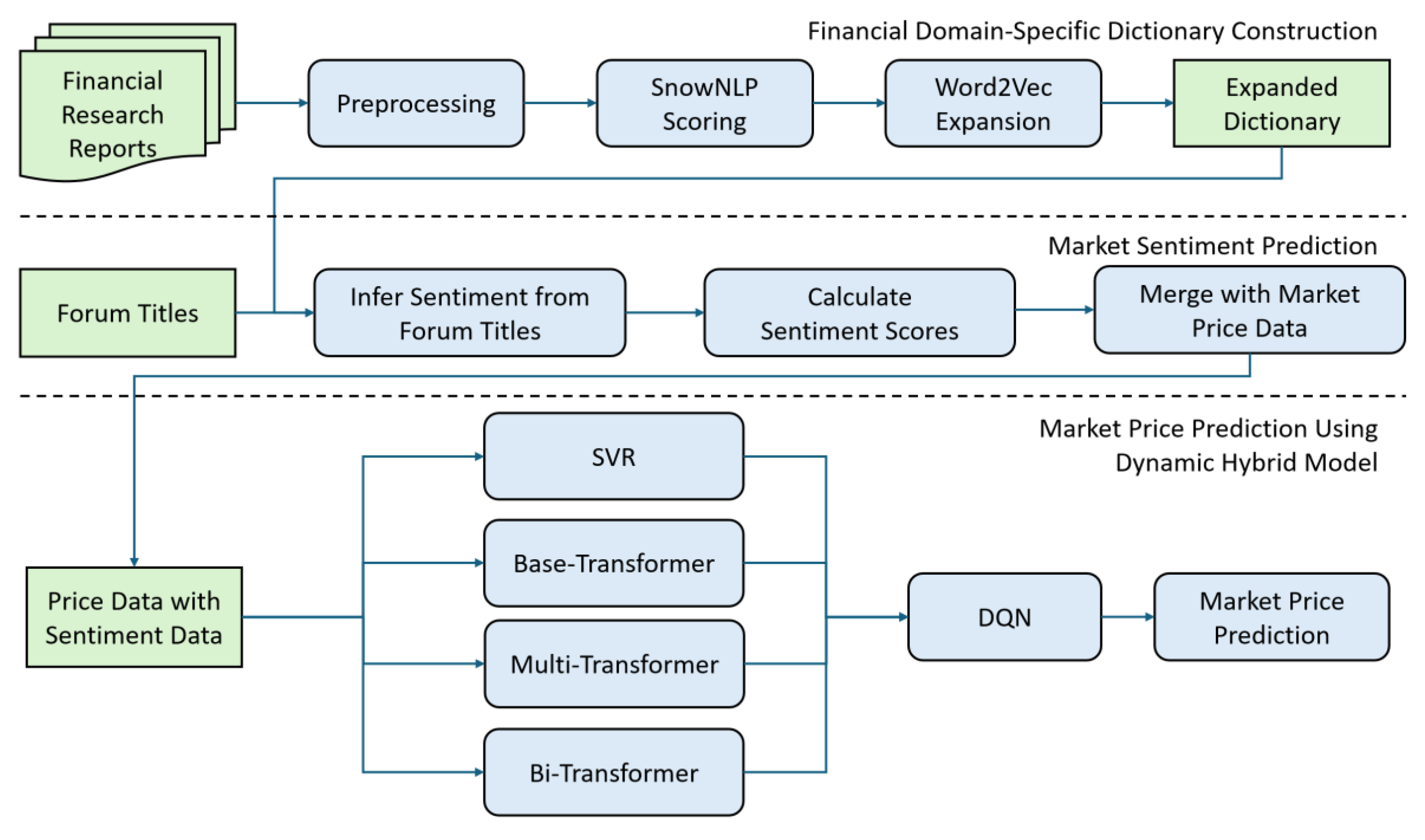
Figure 2.
Heterogeneous feature fusion pipeline for causal price forecasting.
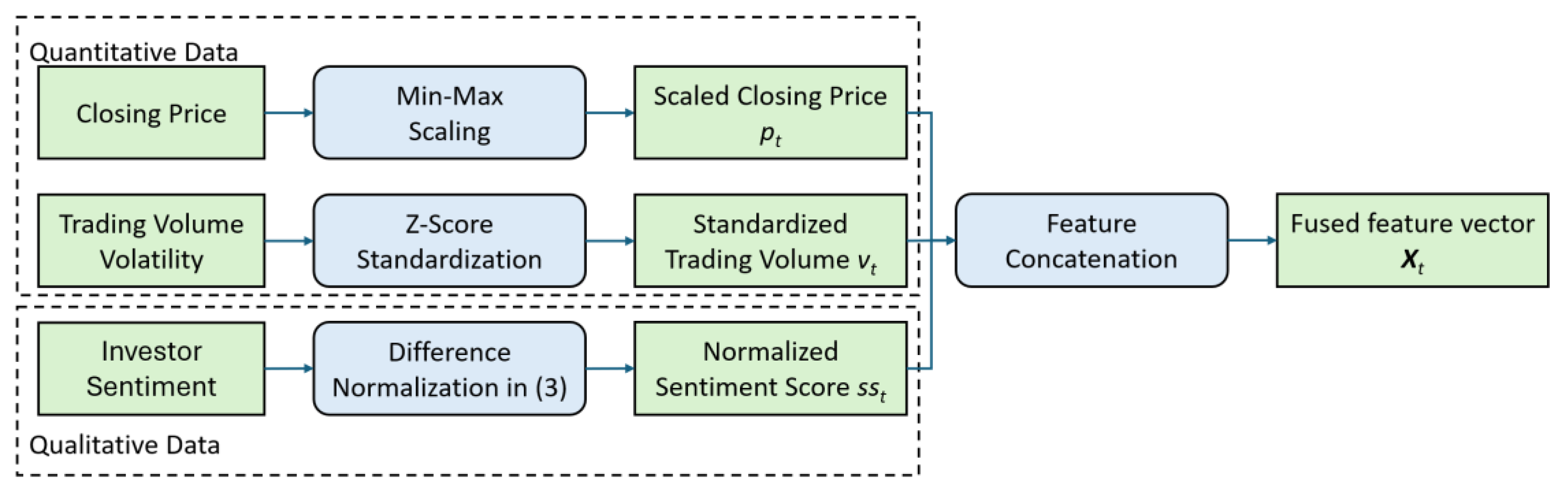
Figure 3.
Model prediction against time on CSI 100 Index.
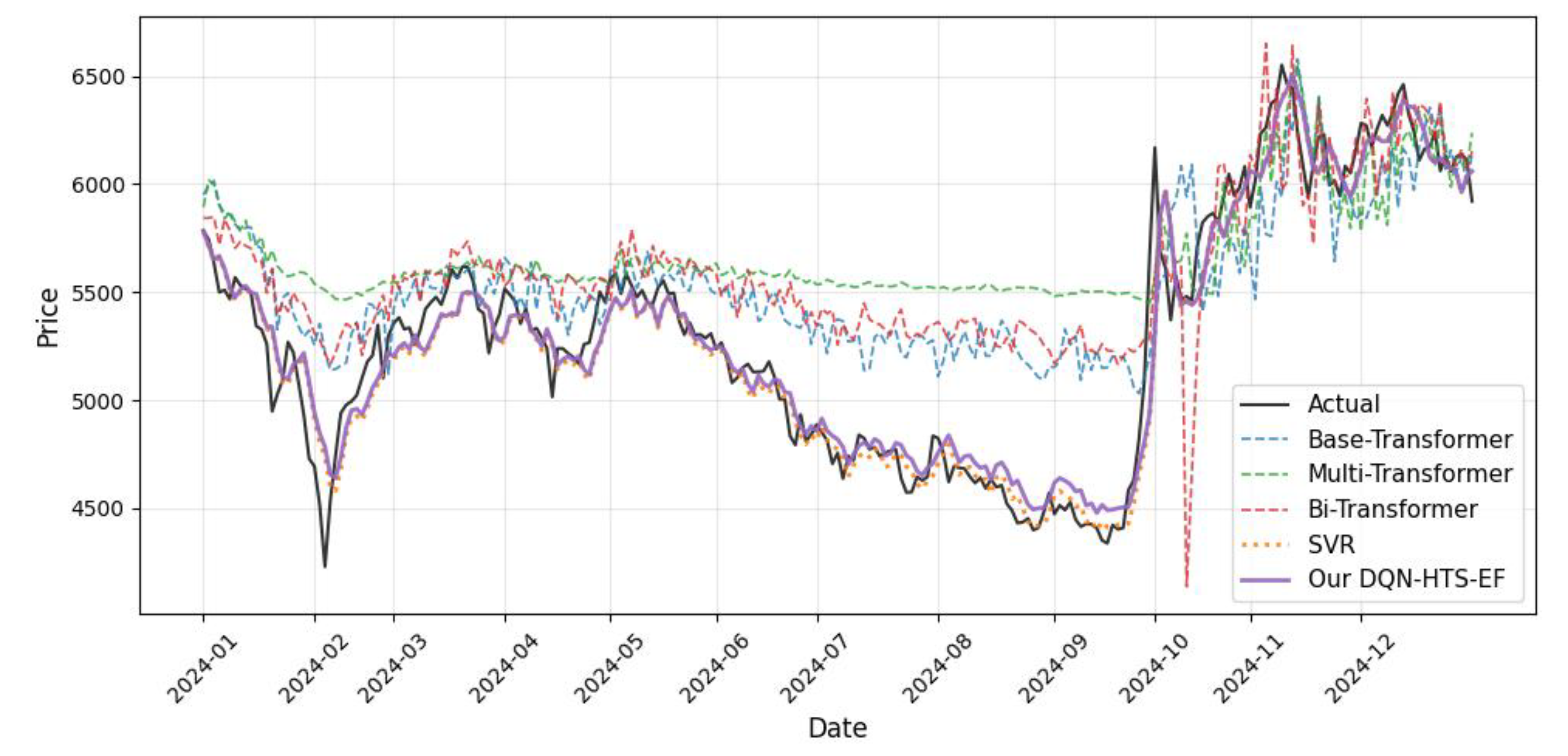
Figure 4.
Model prediction against time on corn futures.
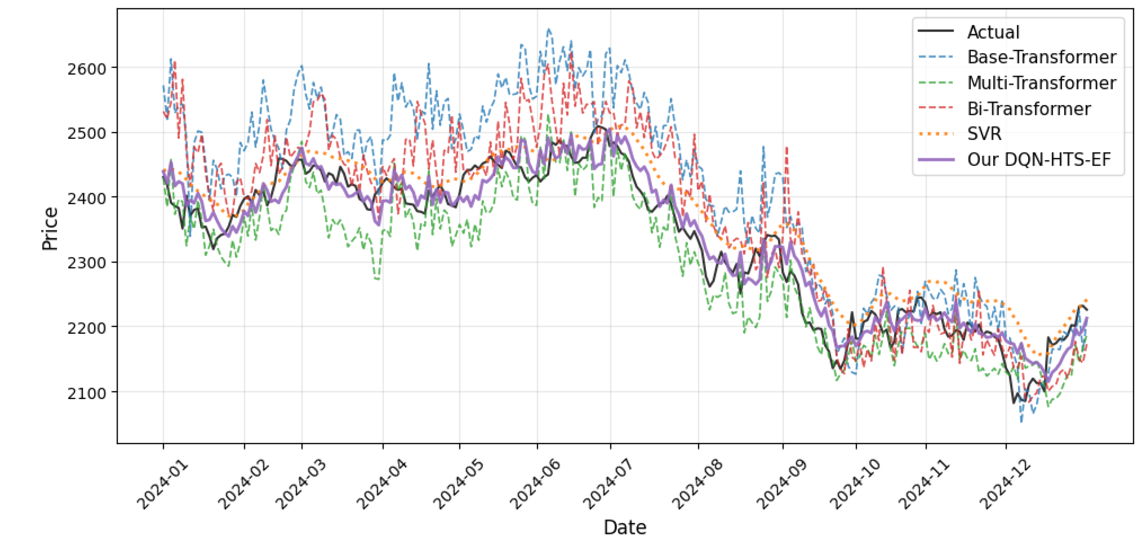
Figure 5.
Model prediction against time on China Unicom Stock.
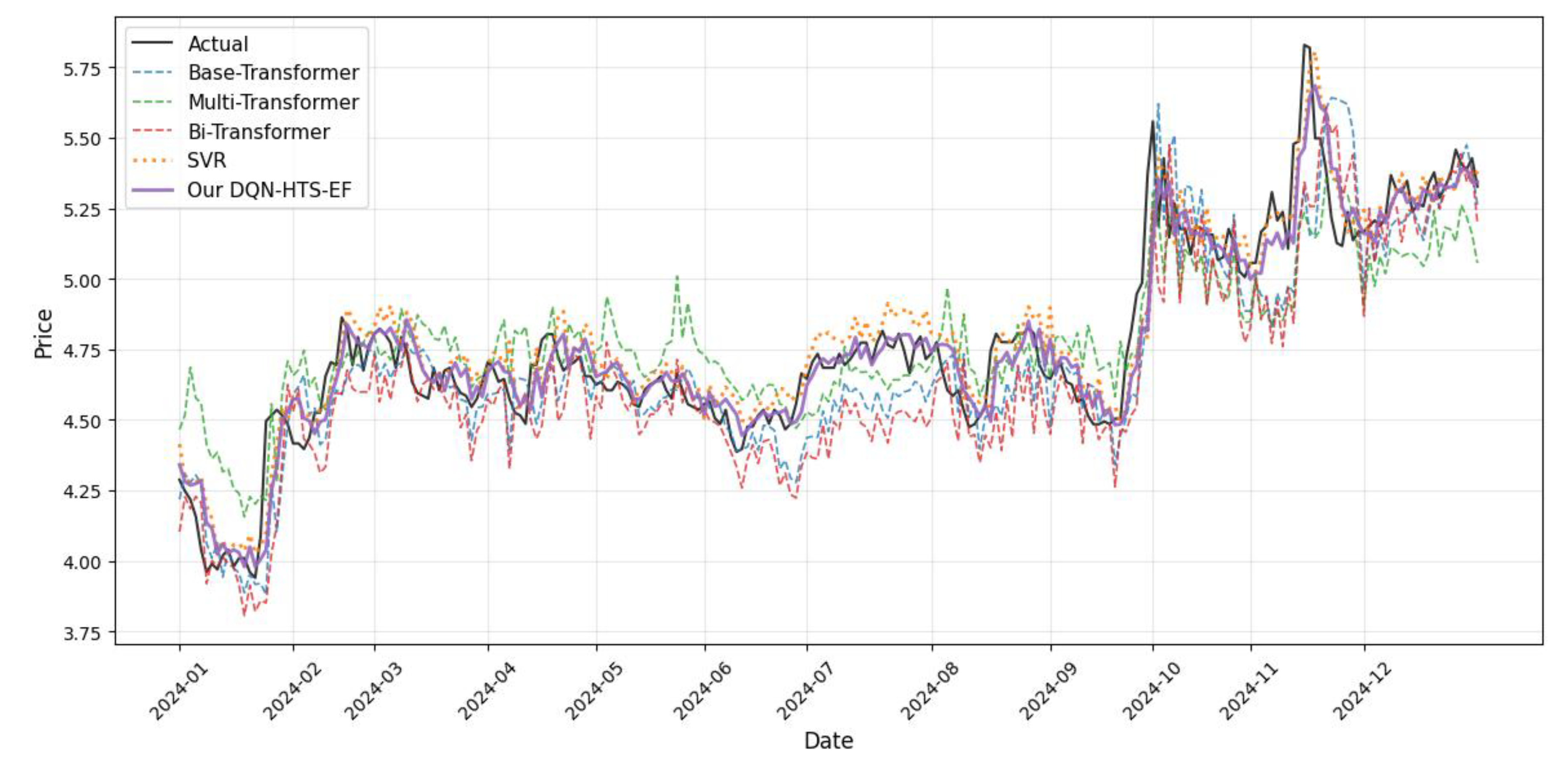
Figure 6.
Model prediction against time on Amazon stock.
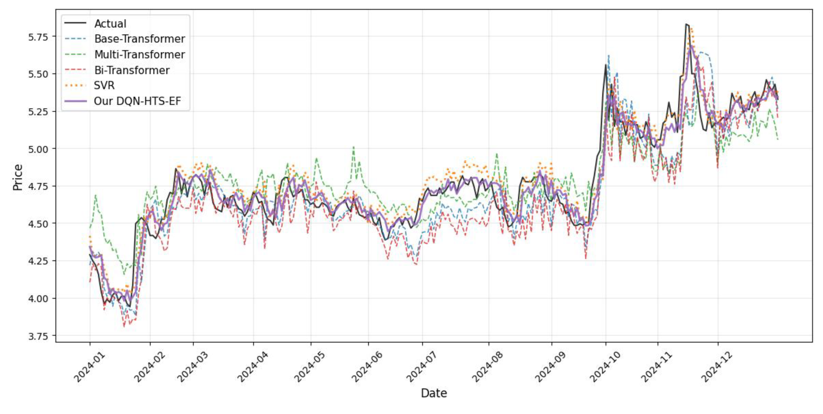

Table 1.
Dataset summary with the details of training and testing periods.
| Commodities | Related Works for the Dataset |
Start Date and End Date |
Train Test Split Ratio |
Test Data Duration |
Important Global Events During Test Period |
|---|---|---|---|---|---|
| CSI 100 Stock Index | [13] | 2024.01.02– 2024.12.31 |
Russia–Ukraine war | ||
| Corn Futures | [6] | 2020.01.01– 2024.12.31 |
80%:20% (969:243) |
||
| China Unicom Stock | [10] | ||||
| AMZN Stock | [10] | 2017.05.25– 2023.04.05 |
70%:30% (1034:442) |
2021.07.06– 2023.04.05 |
COVID-19 pandemic |
Table 2.
Cross-commodity validation of our domain-specific financial sentiment dictionary.
| Commodities | Number of Forum Titles |
Number of Positive Labels (%) |
Number of Negative Labels (%) |
Overall Accuracy (%) |
|---|---|---|---|---|
| CSI 100 Stock Index | 92,184 | 52.57 (48,459) | 9.52 (8,774) | 97.00 |
| Corn Futures | 135,110 | 42.23 (57,055) | 15.75 (21,285) | 97.35 |
| China Unicom Stock | 153,023 | 53.91 (82,491) | 11.12 (16,857) | 97.16 |
| AMZN Stock | 7,382 | 77.43 (5,716) | 6.18 (456) | 90.53 |
Table 3.
Regression analysis for the sentiment score.
| Dataset with Sentiment Score |
Regression Coefficient (Constant) |
Regression Coefficient (Sentiment Score) |
t-value (Constant) |
t-value (Sentiment Score) |
|---|---|---|---|---|
| CSI 100 Stock Index | 6382.353 | 26.888 | 59.624 | 0.105 |
| Corn Futures | 2631.048 | -327.564 | 132.487 | -4.703 |
| China Unicom Stock | 4.541 | -0.488 | 53.235 | -2.450 |
| AMZN Stock | 98.443 | 26.526 | 59.057 | 9.910 |
Table 4.
Model comparison on CSI 100 index dataset.
| Model | MAPE | RMSE | MAE |
|---|---|---|---|
| SVR [13] | 10.9925 | 469.6172 | 393.2344 |
| GRU [13] | 7.8870 | 415.6537 | 353.2755 |
| LSTM [13] | 7.0536 | 382.5686 | 313.8541 |
| FIVMD-LSTM [13] | 2.772 | 154.6032 | 116.5628 |
| GWO-LSTM [14] | 6.0828 | 326.4571 | 265.3836 |
| CEEMDAN-LSTM [5] | 5.2485 | 296.3123 | 233.4450 |
| SSA-BIGRU [2] | 13.6878 | 545.2107 | 501.1394 |
| VMD-SE-GRU [22] | 3.316 | 192.8174 | 148.9184 |
| Proposed DQN-HTS-EF | 2.027 | 148.7959 | 106.9365 |
Table 5.
Model comparison on corn futures dataset.
| Model | MAPE | RMSE | MAE |
|---|---|---|---|
| TCN [6] | 2.532 | 85.720 | 70.128 |
| GRU [6] | 2.347 | 78.946 | 65.015 |
| LSTM [6] | 2.093 | 74.215 | 59.657 |
| SCINet [6] | 1.634 | 55.404 | 45.190 |
| Proposed DQN-HTS-EF | 1.075 | 30.835 | 24.826 |
Table 6.
Model comparison on China Unicom stock dataset.
| Model | MSE | RMSE | MAE |
|---|---|---|---|
| CNN [9] | 0.037 | 0.193 | 0.134 |
| LSTM [18] | 0.036 | 0.189 | 0.128 |
| BiLSTM [19] | 0.035 | 0.189 | 0.132 |
| CNN-LSTM [23] | 0.030 | 0.174 | 0.110 |
| CNN-BiLSTM [23] | 0.029 | 0.170 | 0.110 |
| BiLSTM-ECA [23] | 0.039 | 0.198 | 0.142 |
| CNN-LSTM-ECA [23] | 0.032 | 0.180 | 0.127 |
| CNN-BiLSTM-ECA [23] | 0.028 | 0.167 | 0.103 |
| LSTM-mTrans-MLP [10] | 0.018 | 0.133 | 0.092 |
| Proposed DQN-HTS-EF | 0.012 | 0.108 | 0.075 |
Table 7.
Model comparison on AMZN stock dataset.
| Model | MAE | MSE | RMSE |
|---|---|---|---|
| Linear regression [25] | 72.47 | 7231.59 | 85.04 |
| Exponential Smoothing [8] | 16.62 | 363.83 | 19.074 |
| LSTM [26] | 14.97 | 418.97 | 20.468 |
| CNN-BiLSTM [23] | 4.518 | 28.478 | 5.336 |
| Proposed DQN-HTS-EF | 4.335 | 28.018 | 5.293 |
Table 8.
SHAP Analysis of Sentiment Scores and Model Predictions Across Datasets.
| Dataset | Sentiment Score SHAP Importance |
Dominant Model (Highest SHAP Importance) |
Dominant Model SHAP Importance |
|---|---|---|---|
| CSI 100 Stock Index | 0.0378 | Multi-Transformer | 0.1687 |
| Corn Futures | 0.003 | Bi-Transformer | 0.2289 |
| China Unicom Stock | 0.0088 | SVR | 0.1186 |
| AMZN Stock | 0.0367 | Multi-Transformer and SVR (Tied) |
1.5589 / 1.5510 |
Table 9.
MSE comparison of ensemble strategies on diverse datasets.
| Dataset | Proposed DQN-HTS-EF |
Arithmetic Mean | Weighted Average |
Directional Voting |
|---|---|---|---|---|
| CSI 100 Stock Index | 0.0015 | 0.0087 | 0.0020 | 0.0140 |
| Corn Futures | 0.0008 | 0.0018 | 0.0011 | 0.0036 |
| China Unicom Stock | 0.0117 | 0.0196 | 0.0146 | 0.0287 |
| AMZN Stock | 0.0018 | 0.0025 | 0.0024 | 0.0033 |
Disclaimer/Publisher’s Note: The statements, opinions and data contained in all publications are solely those of the individual author(s) and contributor(s) and not of MDPI and/or the editor(s). MDPI and/or the editor(s) disclaim responsibility for any injury to people or property resulting from any ideas, methods, instructions or products referred to in the content. |
© 2025 by the authors. Licensee MDPI, Basel, Switzerland. This article is an open access article distributed under the terms and conditions of the Creative Commons Attribution (CC BY) license (http://creativecommons.org/licenses/by/4.0/).
Copyright: This open access article is published under a Creative Commons CC BY 4.0 license, which permit the free download, distribution, and reuse, provided that the author and preprint are cited in any reuse.


