Submitted:
16 July 2025
Posted:
17 July 2025
You are already at the latest version
Abstract
Hollow fiber water gap membrane distillation (HF-WGMD) modules are gaining attention for desalination applications due to their compact design and high surface-area-to-volume ratio. This study presents a comprehensive CFD model to analyze and compare the performance of two HF-WGMD module configurations: one with a conventional stagnant water gap (WG) and the other incorporating water gap flow circulation. The model was validated against experimental data, showing excellent agreement, and was then used to simulate flow patterns in the feed, water gap, and coolant domains. Results indicate that, at a feed temperature of 80 °C with a stagnant WG, employing a turbulent flow scheme in the feed side increases permeate flux by 20.7% compared to laminar flow, while increasing coolant flow rate have a minor impact. In contrast, introducing circulation within the water gap significantly enhances performance, boosting permeate flux by 30.1%. This effect becomes more pronounced with rising feed temperature: increasing from 50 °C to 80 °C leads to a flux increase from 6.74 to 27.89 kg/(m²·h) under circulating WG conditions. However, in multi-stage systems, the energy efficiency trade-off becomes evident. Water gap circulation is more energy-efficient than the stagnant configuration only for systems with fewer than 20 stages. At higher stage counts, the stagnant WG setup proves more efficient. For example, at 80 °C and 50 stages, the stagnant configuration consumes just 793 kWh/m³, representing a 47.3% reduction in energy consumption compared to the circulating WG setup. These findings highlight the performance benefits and energy trade-offs of water gap circulation in HF-WGMD systems, providing valuable guidance for optimizing high-efficiency desalination module designs.
Keywords:
Membrane distillation
; Distillate water flux
; Numerical simulation
; Water gap circulation
; Multistage configuration
1. Introduction
Membrane distillation is a thermally driven separation process that leverages vapor pressure differences to facilitate the diffusion of water vapor through a hydrophobic membrane, effectively isolating salts and other impurities. The technique is adaptable to various configurations, each suited to specific applications and offering distinct advantages, such as direct contact membrane distillation (DCMD) [1,2], air gap membrane distillation (AGMD) [3,4], sweeping gas membrane distillation (SGMD) [5,6], and vacuum membrane distillation (VMD) [7,8].
Water gap membrane distillation (WGMD) has emerged as a promising technology for water desalination. In a conventional WGMD configuration, a stagnant layer of distillate water is maintained on the cold side of a hydrophobic membrane, serving as the permeate for the module. Additionally, a cooling fluid is separated from the permeate by a cooling plate, ensuring that the water gap receives adequate cooling. This configuration enhances the water output flux of WGMD compared to air gap membrane distillation (AGMD) systems [9,10,11,12]. Furthermore, WGMD modules exhibit superior thermal efficiency, resulting in lower thermal energy consumption when compared to direct contact membrane distillation (DCMD) modules [13,14].
Numerous studies have investigated the conventional WGMD configuration as a viable technology for desalinating saline water, focusing on enhancing the performance of various WGMD modules [15,16,17]. Lawal et al. [18] conducted experimental investigations to assess the impact of different cooling plate materials on the performance of plate and frame WGMD modules under various feed and coolant operating conditions. In their experiments, the water gap thickness was maintained at 5 mm, the module length at 40 mm and seawater salinity at the feed inlet was considered for all test cases. The results indicated that increasing the thermal conductivity of the cooling plate positively influenced the module’s output flux, achieving a maximum flux of 32 kg/(m2h) when utilizing a copper cooling plate (the most conductive material studied) at feed and coolant inlet temperatures of 70 °C and 15 °C, respectively, with a feed flow rate of 1.2 L/min. The gained output ratio (GOR) of the module was approximately 0.38. Furthermore, reducing the feed flow rate improved the thermal performance of the module, resulting in a GOR of 0.42 at a flow rate of 0.6 L/min, under the same temperature conditions. Notably, the use of a stainless-steel plate yielded a slightly higher GOR of about 0.43 under identical operating conditions. Elsheniti et al. [13] conducted a comparative numerical study between DCMD and WGMD hollow fiber (HF) modules. They developed a two-dimensional axisymmetric transient computational fluid dynamics (CFD) model to simulate the concentrating process of feed water while recirculating through the modules’ feed channels. The study was performed at three different feed tank temperature levels, maintaining the effective module length at 100 mm, with an initial feed salinity of 70000 ppm and permeate (for DCMD) and coolant (for WGMD) inlet temperatures set at 20 °C. The findings indicated that the WGMD desalination system achieved an average water flux of 8.85 kg/(m2h). In comparison, the DCMD system demonstrated a 25.4% increase in flux at a feed tank temperature of 70 °C while concentrating feed water to 233333 ppm. However, WGMD demonstrated superior energy efficiency, with specific thermal energy consumption (STEC) recorded at 903 kWh/m3, compared to 1026 kWh/m3 for the DCMD system under similar conditions while concentrating feed water to 100000 ppm. The GOR for WGMD was 0.72, whereas it was 0.63 for DCMD at the same operational parameters.
Several studies have explored unconventional WGMD modules, such as material gap or conductive gap membrane distillation modules [19,20,21], aimed at enhancing the transport properties of the module gap. Other research efforts have proposed the incorporation of external sources to improve the characteristics of the conventional water gap, such as the use of a rotating impeller [22,23]. For instance, Lawal [22] experimentally examined the performance of a WGMD module equipped with a circulation impeller placed within the water gap to enhance transport characteristics. The study evaluated the effect of impeller rotation speed on the performance of a module with a length of 90.25 mm and a gap thickness of 11 mm at a salinity of 4080 ppm. The results indicated that increasing the impeller speed up to 1100 rev/min significantly improved the overall performance of the module, with a 153.1% increase in flux compared to the conventional WGMD module with a stagnant water gap at feed and coolant inlet temperatures of 70 °C and 20 °C, respectively. Moreover, the STEC of the module was reduced to 1400 kWh/m3, achieving a 12.2% reduction compared to the conventional WGMD module under the same temperature conditions.
Despite ongoing research aimed at enhancing the thermal performance of WGMD systems, significant improvements are still needed. One effective strategy for reducing thermal energy consumption in WGMD modules involves implementing a multistage (MS) arrangement, which incorporates multiple modules in series [24,25,26]. Series connection enables the feed water to be expelled at lower temperature levels while maximizing the distillate water extraction. In the meanwhile, thermal energy gained through the coolant channel is recovered to preheat saline water before it enters the feed channel. For instance, Alawad et al. [27] experimentally investigated the influence of various operating conditions, including feed and coolant inlet temperatures and flow rates, on the thermal performance of a multistage WGMD desalination system. This MS-WGMD system, consisting of four stages arranged in series, was evaluated with a fixed feed inlet salinity of 250 ppm. The study revealed that the four-stage system achieved an STEC of 1543 kWh/m3, representing a 50.6% reduction in STEC compared to a single module at feed and coolant inlet temperatures of 70 °C and 25 °C, respectively. Additionally, the GOR was measured at 0.43, indicating an increase of 104.8% over that of the single module under the same feed and coolant inlet temperatures. Another tactic to make the module more compact, Elbessomy et al. [28] examined the impact of helical configurations of single and double hollow fibers inserted within the cooling tubes on the productivity and thermal performance. The results indicated that single helical fiber modules enhanced water flux by approximately 11.4% at feed and coolant inlet temperatures of 70 °C and 20 °C, respectively, while double helical fibers showed only an 8.07% increase under the same conditions. Furthermore, the study demonstrated that increasing fiber length through helical configuration could reduce the module’s STEC from 6000 kWh/m3 for a straight single fiber to 3900 kWh/m3 for a single fiber with 50 helical turns. Notably, employing up to three stages of helical single fiber modules in series could further decrease the desalination system’s STEC to 1800 kWh/m3.
A review of the literature reveals a gap in CFD simulations addressing the circulating water gap process, particularly within the context of hollow-fiber membrane distillation. Most to date studies focus on conventional stagnant water gap configurations, overlooking the impact of circulation with the hollow fiber membrane configurations. To address this gap, this study develops a theoretical framework and a CFD simulation to implement and analyze the circulating water gap in HF-WGMD modules to be compared with conventional modules. A two-dimensional axisymmetric mathematical model is established, incorporating mass, momentum and energy conservation equations to simulate the transport phenomena across the feed channel, membrane, water gap, cooling tube and coolant stream. The model provides a detailed assessment of temperature and concentration distributions, offering new insights into the influence of water gap circulation against conventional stagnant water gap configuration. A parametric study evaluates key operational factors, including feed and coolant velocities, temperatures and circulating water gap flow rate. Unlike previous studies [13,15,28], the current work investigates the influence of turbulent flow regime for the different module streams on the HF-WGMD module productivity. Furthermore, the performance of a multistage circulating HF-WGMD module is evaluated and compared with that of a conventional stagnant configuration. Comparative analyses based on permeate flux and STEC are carried out to explore the limitations of water gap circulation in enhancing module productivity and thermal efficiency, offering new insights into the design and optimization of high-performance HF-WGMD systems.
2. Stagnant and Circulating Multistage HF-WGMD Systems’ Layout
The HF-WGMD desalination module adopted in the current study features a shell-and-tube configuration, where the feed channels are created by the lumen sides of the hollow fibers within the module. Each hollow fiber is positioned centrally within a cooling tube, which establishes the module distillate water gap. Concurrently, cooling water flows through the shell side of the module. A schematic diagram of the HF-WGMD module is illustrated in Figure 1.
Two configurations of MS-HF-WGMD module will be investigated: the stagnant water gap and circulating water gap. The stagnant module is illustrated in Figure 2 (a), where several HF-WGMD modules are configured in series, with stagnant water in modules’ WG. Cooling water, drawn from an open saline water source, is directed through the shell side of the modules, flowing from the last module to the first. This arrangement enables the recovery of thermal energy from the feed channels via the saline water before it enters the primary feed water heater. Subsequently, the feed water traverses the lumen side of the hollow fibers in the modules, starting from the first module and exiting into a rejected brine tank from the last module, thereby achieving a counter-current flow pattern for both feed and coolant. The distillate water product is collected via overflow from the stagnant water gaps.
On the other hand, Figure 2 (b) depicts a similar feed and coolant flow arrangement for the MS-HF-WGMD module, but with circulation in the water gap. In this configuration, the distillate water is circulating through the gap between the cooling tubes and the hollow fibers of the modules, following a concurrent flow pattern with the feed water. The distillate water product is then collected in a common water tank.
3. Methodology
A 2D axisymmetric model is introduced in this study to simulate the mass, momentum and heat transport physics in HF-WGMD system with both stagnant and circulation water gap configurations. The model is constructed using the fundamental principles of mass, momentum, and energy conservations.
To simplify the computational process while preserving solution accuracy, the following assumptions are considered:
- The hollow fiber membrane and cooling tube are perfectly concentric.
- The hollow fiber membrane exhibits uniform and isotropic porosity.
- Fouling at the feed-membrane interface is neglected.
- Pore wetting within the membrane is assumed to be absent.
- Heat loss from the WGMD module is considered negligible.
The model includes five domains entitled; feed channel, hollow fiber membrane layer, water gap, cooling tube, and cooling channel, as depicted in Figure 3. Whereas the distillate water is considered stagnant in the water gap, Figure 3 (a), it is circulated using an external water pump as shown in Figure 3 (b). Table 1 outlines the defined dimensional parameters and operational conditions of the primary module, offering a detailed summary of the system’s specifications.
3.1. Governing Equations
3.1.1. Mass Transport
The concentration balance is applied for feed and membrane domains to determine the distribution of water concentration. In the feed domain, both convection and diffusion terms are considered in Fick’s law, which is mathematically described as follows:
where, represents the water concentration within the feed channel, and denote the velocity components of the feed flow in the radial and axial directions, respectively. The mutual diffusion coefficient of water and salt, , is determined using the Wilke-Chang equation [29]:
where, is the feed water local temperature, represents the molecular mass of feed solution, is the dynamic viscosity of the feed fluid in cP and is the molecular volume of water in cm3/mol.
Conversely, within the membrane domain, mass transport is governed exclusively by diffusion only, as water vapor molecules pass through the membrane pores via the diffusion mechanism. That is modeled using Fick’s law as follows:
Here, is the local vapor concentration in membrane layer, denotes the diffusion coefficient of water vapor through the membrane.
Diffusion mechanism in hydrophobic membranes is influenced by the characteristics of the transported species in addition to membrane’s intrinsic properties. In MD, the primary transport mechanisms are typically Knudsen diffusion, molecular diffusion, and Poiseuille flow. The effective diffusion mechanisms in the membrane model are identified by calculating the Knudsen number , a dimensionless parameter that quantifies the dominant transport mechanisms, as expressed by the following equation [30]:
Here, is the membrane’s pore diameter, equals to 0.16 μm in the current study, while denotes the mean free path of vapor molecules and can be calculated using the following equation:
In this equation, represents the average membrane temperature, is pressure, and is Boltzmann constant. The molecular collision diameters for air and water are denoted as and, respectively [31]. Additionally, and represent the molecular masses of air and water, respectively and.
In this study, the calculated Knudsen number falls within the transition region , indicating that the diffusion process is influenced by both Knudsen diffusion and ordinary molecular diffusion. The effective diffusion coefficient is then calculated as the combined contribution of these two mechanisms as follows.
where indicates the membrane porosity, and represents the tortuosity of the membrane pores, which can be estimated using the following equation [32]:
The coefficients for Knudsen diffusion and the ordinary diffusion of vapor in air can be determined using the following equations [30]:
3.1.2. Momentum Transport
To obtain the velocity and pressure distributions within the feed, circulating water gap, and cooling channel domains, the governing continuity and Navier-Stokes equations for fluid flow are solved. For 2D-axisymmetric, steady and incompressible, these equations are expressed as follows [33]:
where, and are the fluid density and dynamic viscosity, respectively. is the turbulent viscosity and set to zero in the laminar flow cases while the realizable turbulence model, implemented within COMSOL Multiphysics software, is employed to solve for in the Reynolds-averaged Navier-Stokes (RANS) equations used for turbulent flow cases.
3.1.3. Energy Transport
The temperature distribution is an important factor in the MD process, as it directly impacts the calculations of diffusion coefficients and saturation concentrations. Consequently, the energy conservation equation is solved concurrently with the mass and momentum transport equations to determine the local temperature distribution throughout the entire module. Thermal energy transfer equation, encompassing both convection and conduction, is considered for feed, circulating water gap, and cooling channels and is expressed as follows:
where, is temperature, is the thermal conductivity and is the specific heat of the fluid.
In contrast, only conduction-driven heat transfer is considered in the energy conservation equation for the HF membrane, stagnant water gap, and cooling tube domains and can be presented as follows:
For the membrane layer, the thermal conductivity is determined using the following equation:
Here, represents the thermal conductivity of the Polyvinylidene Fluoride (PVDF) membrane’s solid matrix. denotes the thermal conductivity of water vapor, and it is estimated by the subsequent equation [34]:
3.2. Boundary Conditions
The boundary conditions used with the mass, momentum and energy transport equations are listed in the following tables.
3.2.1. Mass Transport
The boundary conditions for the mass transport equation, applied to both the feed and membrane domains, are summarized in Table 2.
Here, represents water vapor concentration at the feed-membrane interface, denotes water vapor concentration at the membrane-water gap interface. These values correspond to the saturation state of water vapor on both sides of membrane, driven by feed water evaporation at the feed side and vapor condensation at the water gap side. The saturation pressures associated with these concentrations are determined using the Antoine equation [35] as follows:
Here, and represent the saturation pressures at the feed-membrane and membrane-water gap interfaces, respectively. Whereas represents the water mole fraction and refers to the water activity coefficient. Both and are determined as follows [34]:
where, is the mole fraction of salt in the feed solution.
The vapor concentrations at feed-membrane and membrane-water gap interfaces are derived from the corresponding saturation vapor pressures, as in the following equations:
where, represents the saturation concentration of water vapor, is the molecular mass of water, is the atmospheric pressure, is the specific volume of water vapor, is the local temperature at the membrane interfaces, and denotes the vapor content.
3.2.2. Momentum Transport
Table 3 outlines the boundary conditions employed for momentum transport physics across the feed, circulating water gap, and cooling channel domains.
3.2.3. Energy Transport
The energy equation, for all domains, is solved by considering the boundary conditions presented in Table 4.
During the evaporation of water at the feed-membrane interface, latent heat is absorbed from the feed water. On the opposite side of the membrane, the vapor condenses, releasing heat into the water gap. To model this thermal behavior, a heat sink boundary condition is applied at the feed-membrane interface. Whereas, a heat source boundary condition is applied at the membrane-water interface. The corresponding heat values is determined as follows:
where is the diffusive mass flux and is the latent heat of vaporization or condensation which can be determined using the following equation:
where, is the membrane local temperature for both membrane interfaces.
3.3. Specific Thermal Energy Consumption
To assess the thermal performance of the desalination module, STEC is employed as a key indicator. STEC represents the amount of thermal energy consumed by the desalination system per unit mass of produced permeate and is expressed in kWh/m3. It is determined using the following equation:
where denotes the feed mass flow rate in kg/s, represents the specific heat capacity of the feed water, and correspond to the feed inlet and coolant outlet temperatures, respectively, refers to the permeate flux, and is the membrane surface area in m2.
3.4. Solving Technique
The finite element approach built in COMSOL Multiphysics is used to solve the current mathematical model. The transport of mass, momentum and heat across the five domains depicted in Figure 3 is solved by means of COMSOL’s built-in modules. User-defined options and variables are used to integrate the rest of expressions (Eqs. 2, 6-10, 18, and 19).
The entire mathematical model is solved instantaneously across all domains as a totally coupled system. Throughout the analysis, the salt concentration is eliminated from the water gap space and considered to be 35000 ppm at the inlet of the feed channel. As a result, the concentration convection-diffusion balance is used to model the distribution of water and salt concentrations in the feed channel.
3.5. Study on the Number of Grid Elements
The gird independence test is performed on a circulating HF-WGMD module of the length of 100 mm with Reynolds number of 2760, 146 and 2712 in the feed, coolant, and water gap, respectively. The feed inlet temperature is kept at 50 °C with a salinity of 35000 ppm. Three different grid levels (127426, 260320 and 508800 elements) were used to test the CFD in this study. As illustrated in Figure 4, using 260320 of grid elements is excessively satisfactory at which the produced flux deviates only by 0.12% when doubling the number of grid elements to 508800. So that, driving the numerical analysis using 260320 number of grid elements can save the computational time with low level of discretization error.
4. Results and Discussion
4.1. Experimental Validation
The experimental validation of the CFD simulation is achieved by comparing the water flux from a stagnant HF-WGMD module, as proposed by Gao et al. [36], with the numerical flux produced by the same module specifications and operating conditions. The experimental module consisted of 8 hollow fibers centered inside 8 stainless steel tubes with 4.55 and 6.35 mm inner and outer diameters. The feed water was pumped through the lumen side of the hollow fibers of 0.8 and 1.16 mm inner and outer diameters at 0.69 m/s inlet velocity and 10000 ppm inlet salinity. Meanwhile, the cooling water was permitted to pass through the module shell side at 0.012 m/s inlet velocity.
As illustrated in Figure 5, three test cases are considered to validate the current CFD simulation model at different feed inlet temperatures of 40, 50 and 60 °C. The numerical fluxes show excellent agreement with the experimental ones in all test cases. The maximum deviation is encountered at 60 °C feed inlet temperature, at which the percentage deviation of −3.2% is recorded.
The current CFD simulation was previously validated using experimental data of a HF-WGMD module that uses high-density polyethylene cooling tubes instead of stainless steel ones by Elbessomy et al. [15]. In this validation, the model showed great agreement with the experimental results encountering maximum deviation less than 5% for all test cases.
4.2. CFD Simulations
In the following sections, CFD simulations are employed to generate temperature contour plots, which offer a visual representation of the temperature distributions within the various domains of the 100 mm HF-WGMD module operating at a feed inlet salinity of 35000 ppm. This allows for a comprehensive evaluation of the influence of varying operational conditions on the module’s performance. Both laminar and turbulent flow regimes within the feed and cooling channels are analyzed to characterize the temperature polarization across the module. Additionally, the influence of the water gap circulation flow pattern on the temperature distribution within the water gap is examined, highlighting the enhancements facilitated by the circulation in the HF-WGMD module. The temperature gradient across both the membrane and water gap is investigated under different feed inlet temperatures, comparing scenarios with stagnant and circulating flow conditions within the HF-WGMD module. For all cases, a Section 3 mm in length at the mid-point of the module is considered for evaluation.
4.2.1. Feed Water Temperature Distribution at Different Feed Inlet Reynolds Numbers of Stagnant HF-WGMD Module
The effect of feed water inlet velocities on the feed water temperature polarization is investigated and reported, though illustrating the temperature contours inside the feed channel domain of a stagnant HF-WGMD module. The CFD is used to simulate the performance of a stagnant HF-WGMD module at different laminar and turbulent feed inlet Reynolds numbers. While the other operating conditions are kept constant at 50 °C feed inlet temperature, and 2300 coolant inlet Reynolds number. Figure 6 shows the temperature distribution of feed water for laminar feed flow pattern of 460, 1380 and 2300 Reynolds numbers and turbulent flow pattern of 2760, 3680 and 4600 Reynolds numbers. As it is obvious in the figure, the feed water temperature distribution enhances with increasing flow Reynolds number in case of laminar flow pattern due to the enhancement that occurs in heat transfer mechanism. Uniform temperature distribution across the feed channel was observed at the three turbulent Reynolds numbers due to the induced turbulence and mixing of the feed water around the fibers. That gives the superiority to turbulent flow in reducing temperature polarization in the feed channel and hence the module flux can be enhanced.
Table 5 gives data for the average temperature and vapor concentration at the feed-membrane interface for different laminar and turbulent feed Reynolds numbers. As discussed, increasing the feed inlet Reynolds number significantly reduces temperature polarization at the feed-membrane interface. At which, interface temperature enhances from 45.1 °C, at Reynolds number of 460, to 47.2 and 47.9 °C at Reynolds numbers of 1380 and 2300, respectively. That induces water vapor concentration of 3.53, 3.9 and 4.04 mol/m3 at the corresponding Reynolds numbers, respectively. On the other side, higher temperatures are obtained in the turbulent feed flow cases with nearly no change. At which, the interface temperature changes from 49.5 to 49.7 °C when increasing Reynolds number from 2760 to 4600 and hence the average concentration remains almost constant at 4.4 mol/m3, as shown in Table 5.
4.2.2. Water Gap, Cooling Tube, and Cooling Water Temperature Distributions at Different Coolant Inlet Reynolds Numbers of Stagnant HF-WGMD Module
The major function of the cooling water in the WGMD configuration is to provide sufficient cooling to the water gap. So that, the CFD simulation is used to investigate the effect of cooling water Reynolds number on the WG temperature. The study is conducted on a stagnant HF-WGMD module at 50 °C feed inlet temperature while keeping 2300 feed inlet Reynolds number. Figure 7 shows the temperature distribution inside WG, cooling tube and cooling water domains at different laminar (146, 1380 and 2300) and turbulent (2760, 3680 and 4600) Reynolds numbers. It is noticed that coolant Reynolds number has a negligible effect on the WG temperature for all laminar flow cases. Slightly lower temperatures were observed for the water guide and cooling tube at turbulent flow patterns. Hence, it can be deduced that the hydraulic specifications of the cooling channel have minimal effects on the HF-WGMD module flux.
Figure 8 illustrates the average temperature of WG of HF-WGMD module against cooling water Reynolds number. Increasing cooling water laminar Reynolds number from 146 to 2300 decreases the WG temperature from 24.9 to 24 °C representing only 3.6% of enhancement in WG temperature. WG temperature decreases to 23.6 °C when applying turbulent flow pattern in the cooling water, providing maximum WG temperature reduction of 5.2% lower than that at 146 Reynolds number.
4.2.3. WG Temperature Distribution at Different WG Circulation Reynolds Numbers of Circulating HF-WGMD Module
In contrast to the trials to increase the feed and coolant velocities in the previous two sections, the effect of circulating the distillate water on the WG temperature distribution to assess the cooling pattern of membrane-WG interface at different WG Reynolds numbers will be presented in this section. Figure 9 illustrates the temperature contours inside the WG domain of circulating HF-WGMD module at different laminar and turbulent WG Reynolds numbers. The study is conducted on the circulating HF-WGMD module at 50 °C feed inlet temperature and while keeping feed and coolant inlet Reynolds numbers at 2760 and 146, respectively. Although, increasing the flow Reynolds number enhances the heat transfer mechanism at both membrane-WG and WG-cooling tube interfaces, the WG flow layers are arranged with no internal mixing in the laminar flow regime. Hence, the higher WG laminar flow Reynolds number, the higher membrane-WG interface temperature and the lower WG-cooling tube temperature inducing high temperature polarization inside WG domain, as shown in Figure 9 (a), (b) and (c). Increasing the WG Reynolds number to turbulent flow levels () enhances the internal mixing between the flow layers, providing better cooling to membrane-WG interface. No change in WG temperature distribution is observed in all turbulent flow cases, as illustrated in Figure 9 (d), (e) and (f).
Table 6 gives average temperatures and vapor concentrations at the membrane-WG interface at different laminar and turbulent flow Reynolds numbers. Increasing laminar WG Reynolds number from 441 to 2204 increases membrane-WG interface temperature from 31.9 to 34.1 °C which negatively elevates water vapor concentrations from 1.88 to 2.11 mol/m3. While, increasing WG Reynolds number to turbulent flow levels (2712, 5424 and 8136) reduces average temperature nearly to 23 °C in all turbulent cases, providing 27.9% decrease in temperature lower than that at 441 WG Reynolds number. Hence, the water vapor concentration at the membrane-WG interface positively decreases to about 1.15 mol/m3 in all turbulent cases providing water vapor concentration reduction of 38.8% compared to that on 441 WG Reynolds number. That shows the superiority of turbulent WG circulation regime in providing a better cooling pattern for the membrane of HF-WGMD module.
4.2.4. Membrane and WG Temperature Distribution at Different Feed Inlet Temperature of Stagnant and Circulating HF-WGMD Modules
CFD simulations were performed to evaluate the performance of both stagnant and circulating HF-WGMD modules at feed inlet temperatures of 50, 60, 70 and 80 °C. In both configurations, the feed and coolant inlet Reynolds numbers were maintained at 2760 and 146, respectively, while the circulating module was operated at a WG Reynolds number of 2712. Figure 10 shows the temperature distribution through the membrane layer and WG for both configurations. An increase in the feed inlet temperature leads to an elevated feed-membrane interface temperature, which in turn increases the water vapor concentration based on the Antoine equation (Eqs. 18). In the circulating configuration, the introduction of distillate water circulation enhances the mixing between WG layers, reducing the temperature polarization effect near the membrane-WG interface. This is clearly illustrated by the lower temperatures at the membrane cold side in the circulating configuration compared to the stagnant one.
Additionally, Figure 11 compares the average WG temperature between the two configurations. At a 50 °C feed inlet temperature, the WG temperature decreases from 25.3 °C in the stagnant module to 22.8 °C in the circulating module, representing a 9.9% reduction. Higher feed inlet temperatures yield greater reductions, with WG temperature decreases of 13%, 15.5% and 18% at 60, 70 and 80 °C, respectively. These findings demonstrate that the enhanced mixing due to circulation significantly mitigates temperature polarization, thereby improving the overall performance of the HF-WGMD module.
4.3. Parametric Study on a Single Stage of Stagnant and Circulating HF-WGMD Module
The impact of varying operating conditions on the productivity of the HF-WGMD module is examined systematically to identify the best performance parameters. A 100 mm HF-WGMD module, configured with both stagnant and circulating water gaps, is analyzed across a broad range of laminar and turbulent Reynolds numbers, while maintaining fixed inlet feed temperature and salinity conditions of 80 °C and 35000 ppm, respectively. In addition, the performance of the circulating HF-WGMD module is evaluated at different feed inlet temperatures (50, 60, 70 and 80 °C) and compared to the performance of the conventional stagnant HF-WGMD module under the same feed and coolant Reynolds number conditions.
4.3.1. Effect of Feed Flow Reynolds Number on the Water Output Flux of Stagnant HF-WGMD Module
This section examines the distillate water output flux from a stagnant HF-WGMD module under varying laminar and turbulent feed inlet Reynolds numbers. Figure 12 illustrates the relationship between the water flux and the feed inlet Reynolds number at a fixed feed inlet temperature of 80 °C and a coolant inlet temperature of 20 °C. At a feed inlet Reynolds number of 460, the water flux is measured at 13.58 kg/(m2h). As the Reynolds number increases to 1380 and 2300, the water flux correspondingly rises to 16.91 and 18.29 kg/(m2h), representing flux enhancements of 24.5% and 34.7%, respectively. This increase in flux with rising Reynolds number in the laminar regime is attributed to improved convective transport, which mitigates temperature polarization effects at the membrane interface.
Furthermore, the transition from laminar to turbulent flow markedly enhances the water output flux. Specifically, the flux increases from 18.29 kg/(m2h) at a Reynolds number of 2300 (laminar regime) to 22.08 kg/(m2h) at a Reynolds number of 2760, achieving an additional enhancement of 20.7%. Beyond this point, further increases in turbulent Reynolds number yield diminishing returns; for instance, raising the feed Reynolds number from 2760 to 4600 results in only a 3.2% increase in water flux, indicating that the system reaches a near-saturation point in performance improvements under the studied conditions, as illustrated in Figure 12.
Overall, these observations underscore the significant impact of flow regime and Reynolds number on the performance of the HF-WGMD module, particularly in balancing enhanced convective mass transfer with the onset of turbulent flow dynamics.
Figure 12 illustrates the effect of increasing the feed inlet Reynolds number on the pressure drop along the feed channel. As the feed flow remains within the laminar regime, increasing the Reynolds number from 460 to 2300 results in a substantial rise in the pressure drop from 765.5 to 4948.9 Pa. This increase is attributed to the enhanced velocity gradient near the channel walls. Upon reaching the transition regime, where the Reynolds number increases from 2300 to 2760, the pressure drop experiences a further escalation from 4948.9 to 7205.9 Pa, marking a 45.6% increase. This is primarily due to the onset of turbulent eddies and fluctuations, which increase energy dissipation and resistance to fluid motion.
In contrast, operating under fully turbulent conditions leads to a pronounced increase in pressure drop. When the Reynolds number rises from 2760 to 4600, the pressure drop sharply increases to 17640 Pa, representing a significant 144.8% increase. This drastic rise is primarily caused by the intensified turbulence, which amplifies flow resistance. However, despite the substantial increase in pressure drop at high turbulent flow conditions, the corresponding gain in water output flux is found to be negligible, as depicted in Figure 12. This suggests that beyond a certain threshold, further increasing the Reynolds number results in excessive pressure losses without a proportional improvement in system productivity.
4.3.2. Effect of Coolant Flow Reynolds Number on the Water Output Flux of Stagnant HF-WGMD Module
The water output flux of stagnant HF-WGMD module is studied versus cooling water inlet Reynolds number. The investigation is conducted on a stagnant HF-WGMD module at 80 °C feed inlet temperature while keeping 20 °C at coolant inlet. In stagnant HF-WGMD configuration, the cooling channel is separated from the membrane with stagnant WG and cooling tube, which reduces the effect of coolant flow characteristics on the performance of WGMD module. Therefore, no significant enhancement in water flux is observed with increasing coolant inlet Reynolds number in both laminar and turbulent flow regimes, as depicted in Figure 13. At which, HF-WGMD module produces 17.9 kg/(m2h) of water flux at 146 coolant inlet Reynolds number and the flux slightly increases to 18.25 and 18.3 kg/(m2h) when dealing with higher laminar Reynolds numbers of 1380 and 2300. Additionally, transition from laminar to turbulent coolant flow pattern shows no more enhancement in flux at which 18.46 kg/(m2h) of water flux is observed at all turbulent Reynolds numbers.
Moreover, Figure 13 presents the variation in pressure drop along the cooling water channel under both laminar and turbulent flow conditions. At a coolant Reynolds number of 146, the pressure drop is relatively minimal, reaching only 2.7 Pa. However, as the Reynolds number increases, a substantial rise in pressure drop is observed. Specifically, at a Reynolds number of 2300 (the upper limit of the laminar regime) the pressure drop escalates to 90.6 Pa. This increase becomes even more pronounced in the turbulent regime, where the pressure drop reaches 237.2 Pa at a Reynolds number of 4600.
Notably, despite this significant increase in pressure losses, no corresponding enhancement in water output flux is observed, as depicted in Figure 13. This indicates that operating at higher Reynolds numbers in the cooling channel leads to excessive energy dissipation without improving system performance. Consequently, a coolant Reynolds number of 146 appears to be sufficient for maintaining optimal water output flux while minimizing pressure losses, making it the most efficient choice for system operation.
4.3.3. Effect of WG Circulation Reynolds Number on the Water Output Flux of Circulating HF-WGMD Module At Different Feed Inlet Temperatures
In this section, the effect of WG circulation configuration on the module water flux is investigated for a wide range of laminar and turbulent circulation Reynolds numbers at different feed inlet temperatures. Various laminar and turbulent WG Reynolds numbers are tested while keeping the feed and coolant inlet Reynolds numbers of 2760 and 146, respectively. As discussed in Section 4.2.3, in the laminar flow regime, no mixing occurs between WG flow layers, leading to high polarization in temperature and concentration at membrane-WG interface. That provides an unsatisfactory cooling scheme for the membrane cold side and hence negatively affects the module output flux. Therefore, the current study reveals a declining trend in water flux with increasing WG Reynolds number in case of laminar flow regime (), as illustrated in Figure 14. The water flux decreases from 23.31 kg/(m2h) at WG Reynolds number of 441 to 22.31 kg/(m2h) with increasing WG Reynolds number to 2204 representing 4.3% reduction in flux at 80 °C feed inlet temperature. While the flux is 5.41, 9.55 and 15.43 kg/(m2h) for 441 WG Reynolds number and decreases by 8.1%, 6.5% and 5.3% with increasing WG Reynolds number to 2204 at feed inlet temperatures of 50, 60 and 70 °C, respectively.
On the other side, a significant increase in module water flux is observed with the transition from laminar to turbulent flow pattern as a result of enhancement in WG flow characteristics at all feed inlet temperatures. The HF-WGMD module produces 27.89 kg/(m2h) of water flux at 2712 WG Reynolds number attending up to 19.6% of enhancement in water flux over that produced in case of 441 WG Reynolds number (best laminar case) at 80 °C feed inlet temperature, as presented in Figure 14. While higher percentages of enhancement of 24.6%, 21.9 and 20.3% are attended at 50, 60 and 70 °C feed inlet temperatures, respectively. At higher Reynolds numbers, no more increase in water flux is observed due to unchanged flow characteristics, as discussed in Section 4.2.3.
Figure 14 illustrates the variation in WG pressure drop along the WG channel, providing insights into the effectiveness of different WG circulation configurations. The results indicate a substantial increase in pressure drop from 55.8 Pa to 400 Pa as the WG Reynolds number increases within the laminar regime from 441 to 2204, coinciding with a decline in water flux.
Upon transitioning from laminar () to turbulent flow (), the pressure drop exhibits a minor reduction to 390.4 Pa due to improved flow characteristics. However, at higher turbulent Reynolds numbers, a sharp escalation in pressure drop is observed, reaching a peak of 2713.3 Pa at WG Reynolds number of 8136. This significant increase is attributed to intensified frictional losses associated with high-velocity turbulent flow.
Based on the trade-off between flux enhancement and pressure drop, the best WG circulation configuration in this study is determined to be at . Under this condition, the pressure drop per unit water flux is 57.9, 33.5, 21 and 14 Pa/kg/(m2h) which represents a reduction of approximately 28.1%, 25.2%, 23.3% and 21.9% compared to at feed inlet temperatures of 50, 60, 70 and 80 °C, respectively.
4.3.4. Effect of Feed Water Inlet Temperature on the Water Output Flux of Stagnant and Circulating HF-WGMD Modules
A comparative study is performed using CFD simulations to assess the effect of WG circulation configuration on water output flux compared to conventional stagnant HF-WGMD configuration at different feed inlet temperatures. Herein, the HF-WGMD module is simulated with feed and coolant inlet Reynolds numbers of 2760 and 146, respectively, with both stagnant and circulating water gap configurations. In case of circulating HF-WGMD module only, WG is circulated with Reynolds number of 2712. In general, the module productivity is enhanced with increasing feed water temperature due to enhancement in water vapor concentration at feed-membrane interface as depicted in Antione equation (Eqs. 18). The water flux produced by stagnant HF-WGMD module is increased from 5.13 kg/(m2h) at feed inlet temperature of 50 °C to 8.99, 14.38 and 21.43 kg/(m2h) at feed inlet temperatures of 60, 70 and 80 °C, respectively, as illustrated in Figure 15.
Moreover, the water flux is enhanced using circulating WG configuration, as shown in Figuer 15. At feed inlet temperature of 50 °C, the flux is increased to 6.74 kg/(m2h) yielding about 31.4% of distillate water over that produced by the stagnant HF-WGMD module at the same feed inlet conditions. Slightly lower percentages of enhancement are observed at higher feed temperatures. At which, the flux is enhanced by 29.5%, 29.1% and 30.1% at feed inlet temperatures of 60, 70 and 80 °C, respectively, when using circulating HF-WGMD module instead of stagnant HF-WGMD module.
4.4. Performance Assessment of Stagnant and Circulating Multistage HF-WGMD Module
This section evaluates the performance of multistage modules in terms of productivity and energy consumption at different feed inlet temperatures (50, 60, 70 and 80 °C). The coolant inlet temperature is fixed at 20 °C. Reynolds numbers for the feed, coolant and circulating water gap are fixed at 2760, 146 and 2712, respectively. The feed inlet salinity remains constant at 35000 ppm. The study investigates the productivity and thermal performance of HF-WGMD modules connected in series, considering up to 50 stages.
4.4.1. Flux and Energy Recovered
The variations in permeate flux with the number of stages for both stagnant and circulating HF-WGMD configurations at different feed inlet temperatures are presented in Figure 16. The results reveal a general decline in the flux as the number of stages increases for both configurations. This decrease is primarily due to the intensification of temperature and concentration polarization effects while increasing the overall module length, which reduces the driving concentration difference across the membrane.
At a feed inlet temperature of 80 °C, the circulating HF-WGMD module demonstrates an initial performance advantage, achieving a permeate flux of 27.89 kg/(m2h) in a single stage system with 30.1% higher than the 21.4 kg/(m2h) observed in the stagnant configuration. This enhancement is primarily due to improved mixing and convective mass transfer within the water gap. However, this advantage diminishes with additional stages; by the 15th stage, the flux difference narrows to 3.5% and beyond 20 stages, the stagnant module begins to outperform its circulating counterpart. At 50 stages, the stagnant module achieves a 21.9% higher flux (5.76 against 4.5 kg/(m2h)). This trend persists across all tested feed temperatures. For single stage systems at 50, 60 and 70 °C, the circulating module achieves fluxes of 6.7, 11.6 and 18.6 kg/(m2h), outperforming the stagnant module’s 5.1, 9.0, and 14.4 kg/(m2h), respectively. Conversely, at 50 stages, the stagnant module exhibits superior fluxes of 1.8, 2.9, and 4.2 kg/(m2h), compared to 1.5, 2.3, and 3.3 kg/(m2h) for the circulating module at the same temperatures.
Furthermore, Figure 16 illustrates the cooling water temperature rise, an indicator of thermal energy recovery, as a function of the number of stages. For stage counts below 20, both the circulating and stagnant configurations exhibit increasing temperature rise, with the circulating module showing higher values and a steeper growth rate. At a feed inlet temperature of 80 °C and 5 stages, the circulating module achieves a temperature rise of 12.85 °C, 33.4% higher than the stagnant module’s 9.63 °C. However, this advantage diminishes with additional stages; by 20 stages, both configurations converge at approximately 25 °C. Beyond this point, the temperature rise in the circulating module plateaus around 28 °C, while the stagnant module continues to increase, ultimately surpassing the circulating configuration. At 50 stages and 80 °C, the stagnant module records a 36% higher temperature rise. This behavior is consistent across lower feed temperatures. For instance, at 50 stages, the stagnant module outperforms the circulating module by 29.5%, 31.6% and 33.7% at feed temperatures of 50, 70 and 80 °C, respectively, confirming that the stagnant configuration becomes more thermally efficient at high stage counts.
4.4.2. Specific Thermal Energy Consumption
The STEC of the stagnant and circulating MS-HF-WGMD systems is analyzed and presented for different numbers of stages and different feed inlet temperatures, as shown in Figure 17. In both configurations, STEC decreases with increasing number of stages, primarily due to enhanced system productivity from extended module length and improved thermal energy recovery by the coolant, which reduces the energy required to heat the feed stream. At 80 °C, the STEC in the circulating module drops from 20349 to 1402 kWh/m3 as the number of stages increases from 1 to 50, while the stagnant module shows a decrease from 26945 to 793 kWh/m3. For fewer than 20 stages, the circulating module exhibits lower STEC than the stagnant one, indicating superior thermal performance. However, beyond 20 stages, the stagnant configuration achieves a more rapid reduction in STEC. As shown in Figure 17 (d), at 50 stages, the stagnant module consumes approximately 47.3% less thermal energy than the circulating module to produce the same amount of distillate water. This crossover behavior is consistent across all tested feed temperatures [Figure 17 (a–c)], highlighting the diminishing benefit of circulation with increasing stage number.
5. Conclusions
A 2D axisymmetric CFD model is established to simulate the circulation of distillate water through water gap of a HF-WGMD module. The proposed circulating HF-WGMD module performance is assessed and compared with that of conventional HF-WGMD module with stagnant water gap configuration at different feed temperatures. The impact of feed and coolant inlet Reynolds number on the MD module is investigated. The HF-WGMD module with WG circulation configuration is tested for different laminar and turbulent circulation Reynolds numbers. In addition, a study on a multistage system level is implemented for both WG configurations. The following succinctly describes the primary findings of the current study:
- Transitioning from laminar to turbulent feed flow regime assures up to 20.7% more distillate flux when a stagnant WG configuration at feed inlet temperature of 80 °C is considered.
- Increasing coolant inlet Reynolds number has nearly no effect on the module productivity in both laminar and turbulent flow regimes.
- In circulating HF-WGMD modules, increasing WG Reynolds number within the laminar regime reduces flux, while flux remains stable across all turbulent flow conditions.
- Transitioning from laminar to turbulent WG circulation boosts productivity; at , the circulating HF-WGMD module achieves 27.89 kg/(m2h) flux representing 19.6% higher than at , under 80 °C feed temperature.
- At all feed inlet temperatures, utilizing a single stage of circulation WG configuration outperforms the stagnant WG configuration in terms of water output flux, at which the water flux is enhanced by up to 31.4% at 50 °C feed inlet temperature.
- For multi-stage HF-WGMD systems, modules with circulating WG outperform stagnant ones below 20 stages, but the stagnant configuration becomes superior in flux and STEC beyond this threshold.
- At 80 °C, a 50-stage stagnant WG system consumes only 793 kWh/m3, representing a 47.3% reduction compared to circulating WG.
Author Contributions
Conceptualization, M.O.E. and M.B.E.; Methodology, M.O.E. and M.B.E.; Software, M.O.E., K.W.F. and M.B.E.; Validation, M.O.E. and K.W.F.; Formal analysis, M.O.E., K.W.F., M.B.E. and A.R.; Investigation, M.O.E., K.W.F., M.B.E., A.R. and O.A.E.; Data curation, M.O.E. and M.B.E.; Writing—original draft, M.O.E. and K.W.F.; Writing—review & editing, A.R., M.B.E. and O.A.E.; Visualization, S.M.E. and A.R.; Supervision, M.B.E., S.M.E. and O.A.E.; Funding acquisition, M.B.E. All authors have read and agreed to the published version of the manuscript.
Nomenclature
| Water activity coefficient | |
| Specific heat at constant pressure [J/(kg K)] | |
| Concentration [mol/m3] | |
| Diffusion coefficient [m2/s] | |
| Knudsen diffusion coefficient [m2/s] | |
| Ordinary molecular diffusion coefficient [m2/s] | |
| Diameter [m] | |
| Pore diameter [m] | |
| Latent heat of vaporization [J/kg] | |
| Product water flux [kg/m2h] | |
| Knudsen number | |
| Thermal conductivity [W/(m K)] | |
| Module length [m] | |
| Molecular mass [g/mol] | |
| Pressure [Pa] | |
| Concentration in parts per millions | |
| Absorbed/expelled heat flux [W/m2] | |
| Half of center-to-center distance [m] | |
| Radius [mm] | |
| Universal gas constant [J/(mol K)] | |
| Specific thermal energy consumption [kWh/m3] | |
| Temperature [℃] | |
| U | Flow stream mean velocity [m/s] |
| Velocity component in radial direction [m/s] | |
| Specific volume [m3/kg] | |
| Vapor content [kgv/kga] | |
| Velocity component in axial direction [m/s] | |
| Salt mole fraction | |
| Water mole fraction | |
| Air | |
| Atmospheric | |
| Coolant channel | |
| Feed channel | |
| Water gap | |
| Inlet | |
| Membrane | |
| Outlet | |
| Radial direction | |
| Saturation | |
| Cooling tube | |
| Vapor | |
| Water | |
| Axial direction | |
| Membrane porosity | |
| Fluid dynamic viscosity [Pa s] | |
| Fluid density [kg/m3] | |
| Molecule collision diameter [m] | |
| Membrane tortuosity |
References
- Ho, C.-D.; Chiang, M.-S.; Ng, C.A. Performance Analysis of DCMD Modules Enhanced with 3D-Printed Turbulence Promoters of Various Hydraulic Diameters. Membranes 2025, 15, 144. [Google Scholar] [CrossRef] [PubMed]
- Kandi, A.; Mohammed, H.A.; Khiadani, M.; Shafieian, A. The effect of turbulence promoters on DCMD process: A comprehensive review. Journal of Water Process Engineering 2025, 69, 106810. [Google Scholar] [CrossRef]
- Bi, H.; Yuan, H.; Xu, Z.; Liang, Z.; Du, Y. Research on the Performance and Computational Fluid Dynamics Numerical Simulation of Plate Air Gap Membrane Distillation Module. Membranes 2024, 14, 162. [Google Scholar] [CrossRef] [PubMed]
- Mesquita, C.R.S.; Gómez, A.O.C.; Cotta, C.P.N.; Cotta, R.M. Comparison of Different Polymeric Membranes in Direct Contact Membrane Distillation and Air Gap Membrane Distillation Configurations. Membranes 2025, 15, 91. [Google Scholar] [CrossRef] [PubMed]
- Elsheniti, M.B.; Elbessomy, M.O.; Wagdy, K.; Elsamni, O.A.; Elewa, M.M. Augmenting the distillate water flux of sweeping gas membrane distillation using turbulators: A numerical investigation. Case Studies in Thermal Engineering 2021, 26, 101180. [Google Scholar] [CrossRef]
- Elsheniti, M.B.; Ibrahim, A.; Elsamni, O.; Elewa, M. Experimental and economic investigation of sweeping gas membrane distillation/pervaporation modules using novel pilot scale device. Separation and Purification Technology 2023, 310, 123165. [Google Scholar] [CrossRef]
- Alwatban, A.M.; Alhazmi, M.A.; Aljumaily, M.M.; Alsalhy, Q.F. Computational fluid dynamics simulations of desalination processes in vacuum membrane distillation. Desalination and Water Treatment 2025, 322, 101174. [Google Scholar] [CrossRef]
- Najib, A.; Mana, T.; Ali, E.; Al-Ansary, H.; Almehmadi, F.A.; Alhoshan, M. Experimental Investigation on the Energy and Exergy Efficiency of the Vacuum Membrane Distillation System with Its Various Configurations. Membranes 2024, 14, 54. [Google Scholar] [CrossRef] [PubMed]
- Khalifa, A.E. Water and air gap membrane distillation for water desalination – An experimental comparative study. Separation and Purification Technology 2015, 141, 276–284. [Google Scholar] [CrossRef]
- Amaya-Vías, D.; Nebot, E.; López-Ramírez, J.A. Comparative studies of different membrane distillation configurations and membranes for potential use on board cruise vessels. Desalination 2018, 429, 44–51. [Google Scholar] [CrossRef]
- Khalifa, A.E.; Alawad, S.M. Air gap and water gap multistage membrane distillation for water desalination. Desalination 2018, 437, 175–183. [Google Scholar] [CrossRef]
- Im, B.-G.; Francis, L.; Santosh, R.; Kim, W.-S.; Ghaffour, N.; Kim, Y.-D. Comprehensive insights into performance of water gap and air gap membrane distillation modules using hollow fiber membranes. Desalination 2022, 525, 115497. [Google Scholar] [CrossRef]
- Elsheniti, M.B.; Elbessomy, M.O.; Rezk, A.; Fouly, A.; Elsherbiny, S.M.; Elsamni, O.A. Comparative analyses of transient batch operations of hollow-fiber DCMD and WGMD desalination systems at high salinity levels. Desalination 2025, 600, 118492. [Google Scholar] [CrossRef]
- Gao, L.; Zhang, J.; Gray, S.; Li, J.-D. Experimental study of hollow fiber permeate gap membrane distillation and its performance comparison with DCMD and SGMD. Separation and Purification Technology 2017, 188, 11–23. [Google Scholar] [CrossRef]
- Elbessomy, M.O.; Elsamni, O.A.; Elsheniti, M.B.; Elsherbiny, S.M. Optimum configurations of a compact hollow-fiber water gap membrane distillation module for ultra-low waste heat applications. Chemical Engineering Research and Design 2023, 195, 218–234. [Google Scholar] [CrossRef]
- Alawad, S.M.; Khalifa, A.E.; Abido, M.A.; Antar, M.A. Differential evolution optimization of water gap membrane distillation process for water desalination. Separation and Purification Technology 2021, 270, 118765. [Google Scholar] [CrossRef]
- Im, B.-G.; Woo, S.-Y.; Ham, M.-G.; Ji, H.; Kim, Y.-D. A novel approach to detailed modeling and simulation of water-gap membrane distillation: Establishing a numerical baseline model. Journal of Membrane Science 2025, 715, 123482. [Google Scholar] [CrossRef]
- Lawal, D.U.; Abdulazeez, I.; Alsalhy, Q.F.; Usman, J.; Abba, S.I.; Mansir, I.B.; Sathyamurthy, R.; Kaleekkal, N.J.; Imteyaz, B. Experimental Investigation of a Plate–Frame Water Gap Membrane Distillation System for Seawater Desalination. Membranes 2023, 13, 804. [Google Scholar] [CrossRef] [PubMed]
- Memon, S.; Im, B.-G.; Lee, H.-S.; Kim, Y.-D. Comprehensive experimental and theoretical studies on material-gap and water-gap membrane distillation using composite membranes. Journal of Membrane Science 2023, 666, 121108. [Google Scholar] [CrossRef]
- Swaminathan, J.; Chung, H.W.; Warsinger, D.M.; AlMarzooqi, F.A.; Arafat, H.A.; Lienhard V, J.H. Energy efficiency of permeate gap and novel conductive gap membrane distillation. Journal of Membrane Science 2016, 502, 171–178. [Google Scholar] [CrossRef]
- Cai, J.; Yin, H.; Guo, F. Transport analysis of material gap membrane distillation desalination processes. Desalination 2020, 481, 114361. [Google Scholar] [CrossRef]
- Lawal, D.U. Performance enhancement of permeate gap membrane distillation system augmented with impeller. Sustainable Energy Technologies and Assessments 2022, 54, 102792. [Google Scholar] [CrossRef]
- Lawal, D.U.; Alawad, S.; Usman, J.; Abba, S.I.; Sekar, S.; Mansir, I.B.; Baroud, T.; Alsalhy, Q.F.; Yassin, M.A.; Shah, S.M.H.; et al. Performance assessment of a modified air-gap and water-gap membrane distillation systems. Desalination and Water Treatment 2024, 317, 100303. [Google Scholar] [CrossRef]
- Alawad, S.M.; Khalifa, A.E. Development of an efficient compact multistage membrane distillation module for water desalination. Case Studies in Thermal Engineering 2021, 25, 100979. [Google Scholar] [CrossRef]
- Amaya-Vías, D.; López-Ramírez, J.A.; Gray, S.; Zhang, J.; Duke, M. Diffusion behavior of humic acid during desalination with air gap and water gap membrane distillation. Water Research 2019, 158, 182–192. [Google Scholar] [CrossRef] [PubMed]
- Alawad, S.M.; Lawal, D.U.; Khalifa, A.E.; Aljundi, I.H.; Antar, M.A.; Baroud, T.N.; Eltoum, M.A.M. Optimization and design analysis of multistage water gap membrane distillation for cost-effective desalination. Desalination 2023, 566, 116894. [Google Scholar] [CrossRef]
- Alawad, S.M.; Khalifa, A.E.; Antar, M.A.; Abido, M.A. Experimental Evaluation of a New Compact Design Multistage Water-Gap Membrane Distillation Desalination System. Arabian Journal for Science and Engineering 2021, 46, 12193–12205. [Google Scholar] [CrossRef]
- Elbessomy, M.O.; Elsheniti, M.B.; Elsherbiny, S.M.; Rezk, A.; Elsamni, O.A. Productivity and Thermal Performance Enhancements of Hollow Fiber Water Gap Membrane Distillation Modules Using Helical Fiber Configuration: 3D Computational Fluid Dynamics Modeling. Membranes 2023, 13, 843. [Google Scholar] [CrossRef] [PubMed]
- Poling, B.E.; Prausnitz, J.M.; O’connell, J.P. The properties of gases and liquids; Mcgraw-hill New York: 2001; Volume 5.
- Curcio, E.; Drioli, E. Membrane Distillation and Related Operations—A Review. Separation & Purification Reviews 2005, 34, 35–86. [Google Scholar] [CrossRef]
- Cussler, E.L.; Cussler, E.L. Diffusion: mass transfer in fluid systems; Cambridge university press: 2009.
- Alkhudhiri, A.; Darwish, N.; Hilal, N. Membrane distillation: A comprehensive review. Desalination 2012, 287, 2–18. [Google Scholar] [CrossRef]
- Versteeg, H.K. An introduction to computational fluid dynamics the finite volume method, 2/E.; Pearson Education India: 2007.
- Chen, T.-C.; Ho, C.-D.; Yeh, H.-M. Theoretical modeling and experimental analysis of direct contact membrane distillation. Journal of Membrane Science 2009, 330, 279–287. [Google Scholar] [CrossRef]
- Felder, R.M.; Rousseau, R.W.; Bullard, L.G. Elementary principles of chemical processes; John Wiley & Sons: 2020.
- Gao, L.; Zhang, J.; Gray, S.; Li, J.-D. Modelling mass and heat transfers of Permeate Gap Membrane Distillation using hollow fibre membrane. Desalination 2019, 467, 196–209. [Google Scholar] [CrossRef]
Figure 1.
Schematic diagram of the HF-WGMD module with circulating water gap.
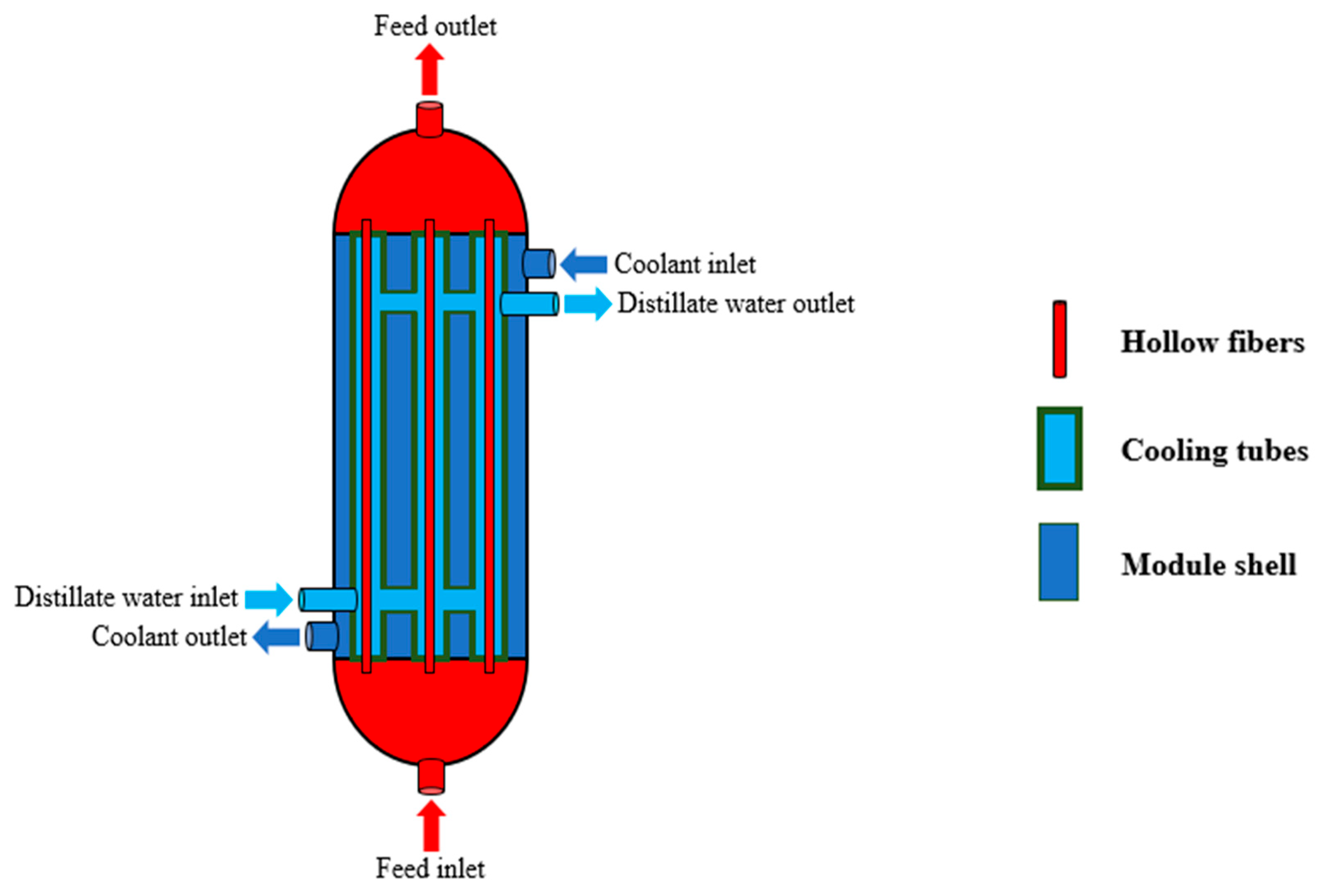
Figure 2.
Schematic diagrams for the configurations of multistage HF-WGMD modules with (a) stagnant WG and (b) circulating WG.
Figure 2.
Schematic diagrams for the configurations of multistage HF-WGMD modules with (a) stagnant WG and (b) circulating WG.

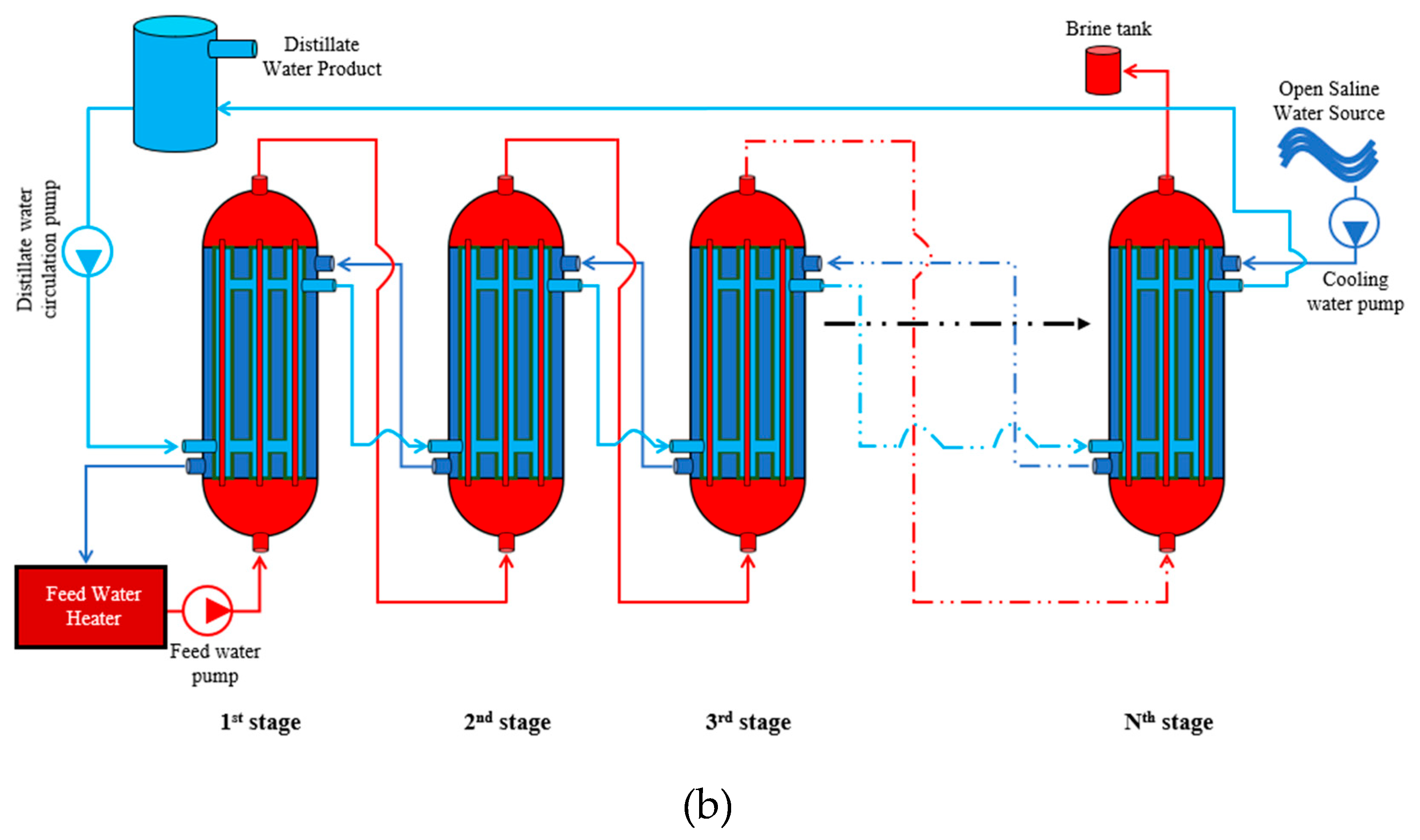
Figure 3.
Schematic diagrams of the simulated domains of HF-WGMD modules; (a) stagnant WG and (b) circulating WG.
Figure 3.
Schematic diagrams of the simulated domains of HF-WGMD modules; (a) stagnant WG and (b) circulating WG.
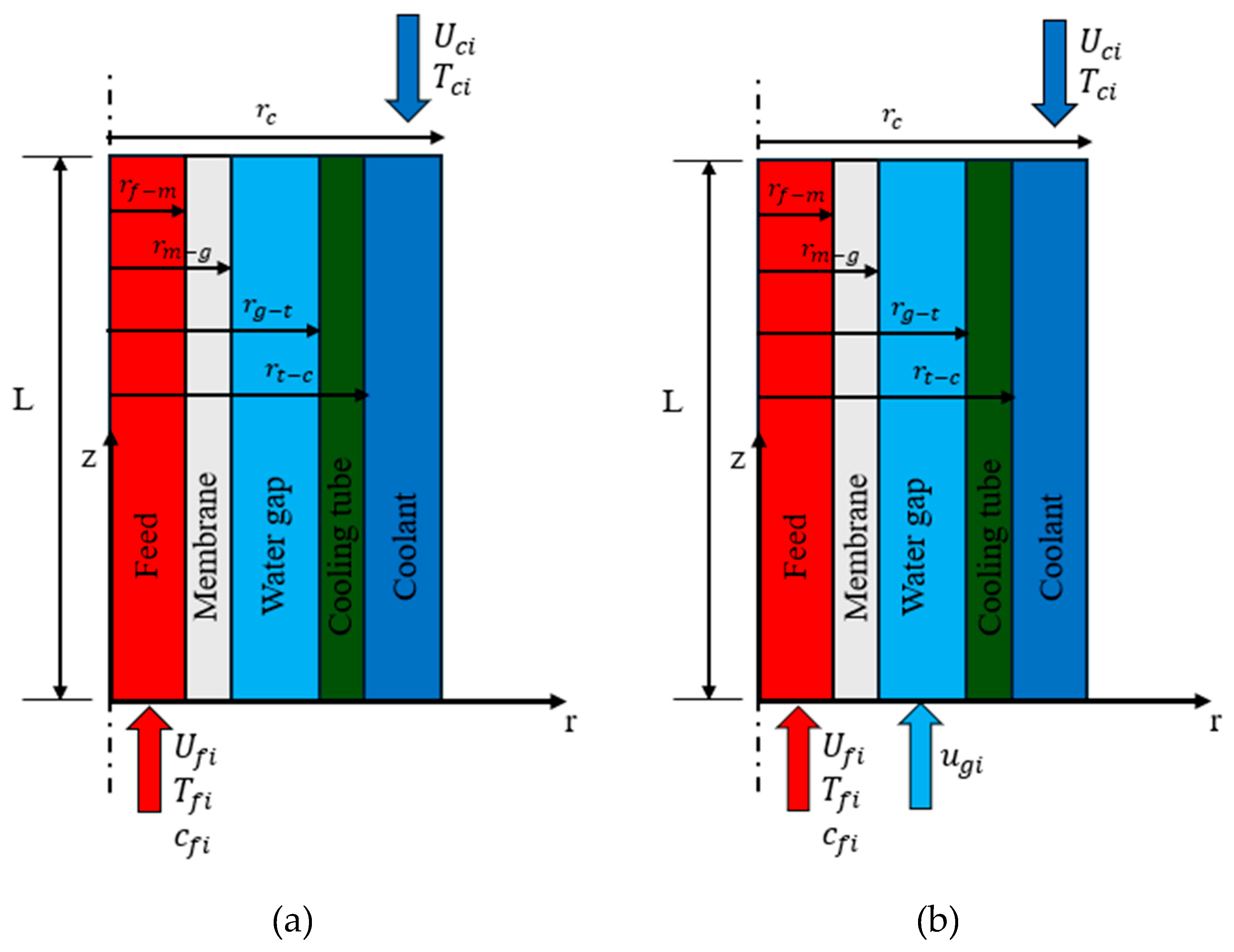
Figure 4.
The grid independence study of the CFD simulation model for a circulating () HF-WGMD module of , and .
Figure 4.
The grid independence study of the CFD simulation model for a circulating () HF-WGMD module of , and .
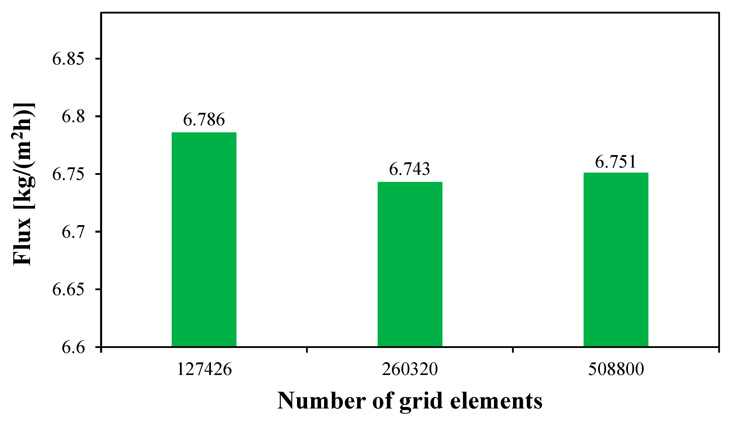
Figure 5.
Experimental validation of the CFD simulation model.
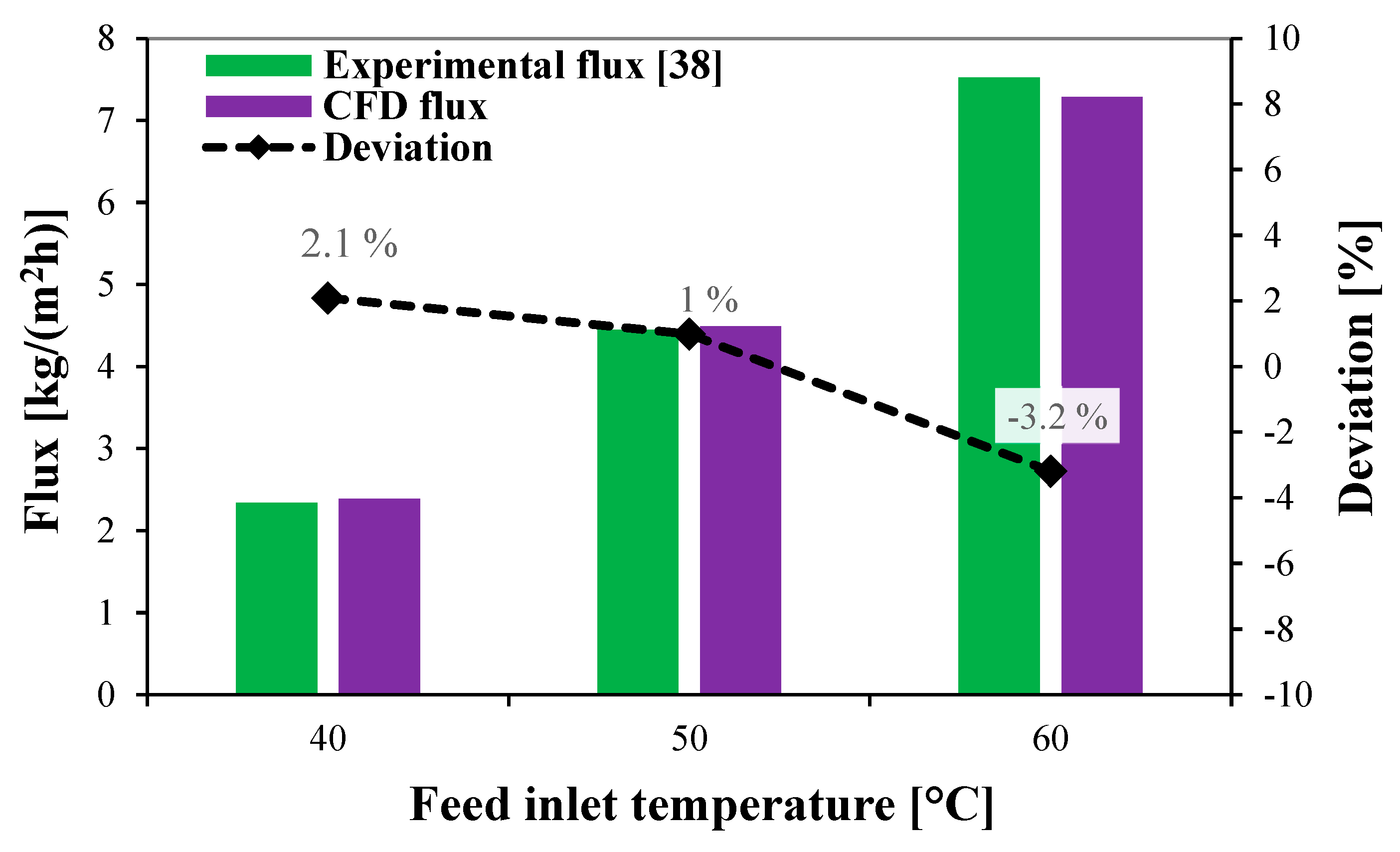
Figure 6.
Temperature distribution of the feed channel of the stagnant HF-WGMD module for different feed Reynolds numbers at and .
Figure 6.
Temperature distribution of the feed channel of the stagnant HF-WGMD module for different feed Reynolds numbers at and .
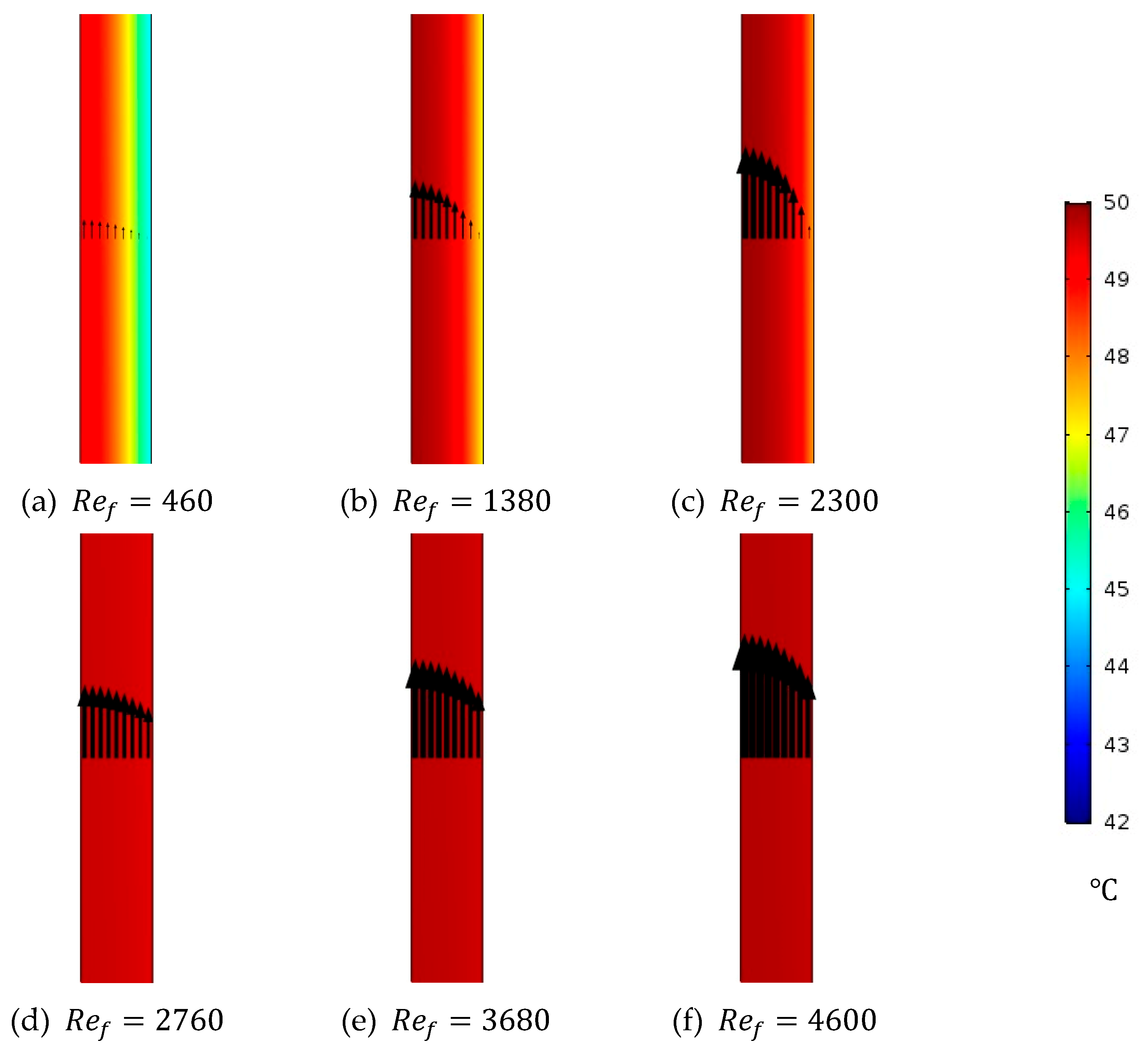
Figure 7.
Temperature distribution of WG, cooling tube and cooling water through the stagnant HF-WGMD module for different coolant Reynolds numbers at and .
Figure 7.
Temperature distribution of WG, cooling tube and cooling water through the stagnant HF-WGMD module for different coolant Reynolds numbers at and .
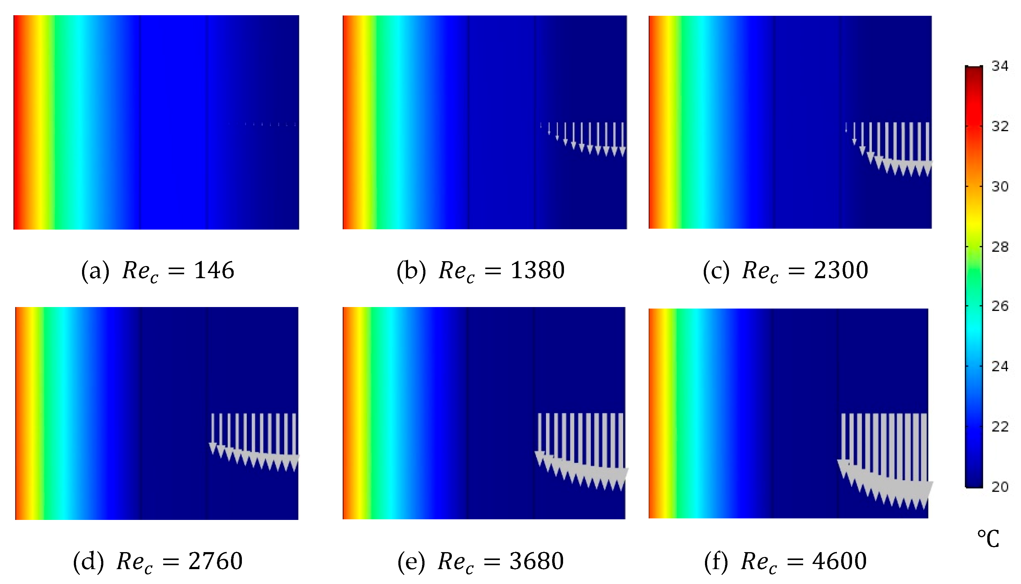
Figure 8.
Average WG temperature of the stagnant HF-WGMD module versus coolant Reynolds number at and .
Figure 8.
Average WG temperature of the stagnant HF-WGMD module versus coolant Reynolds number at and .
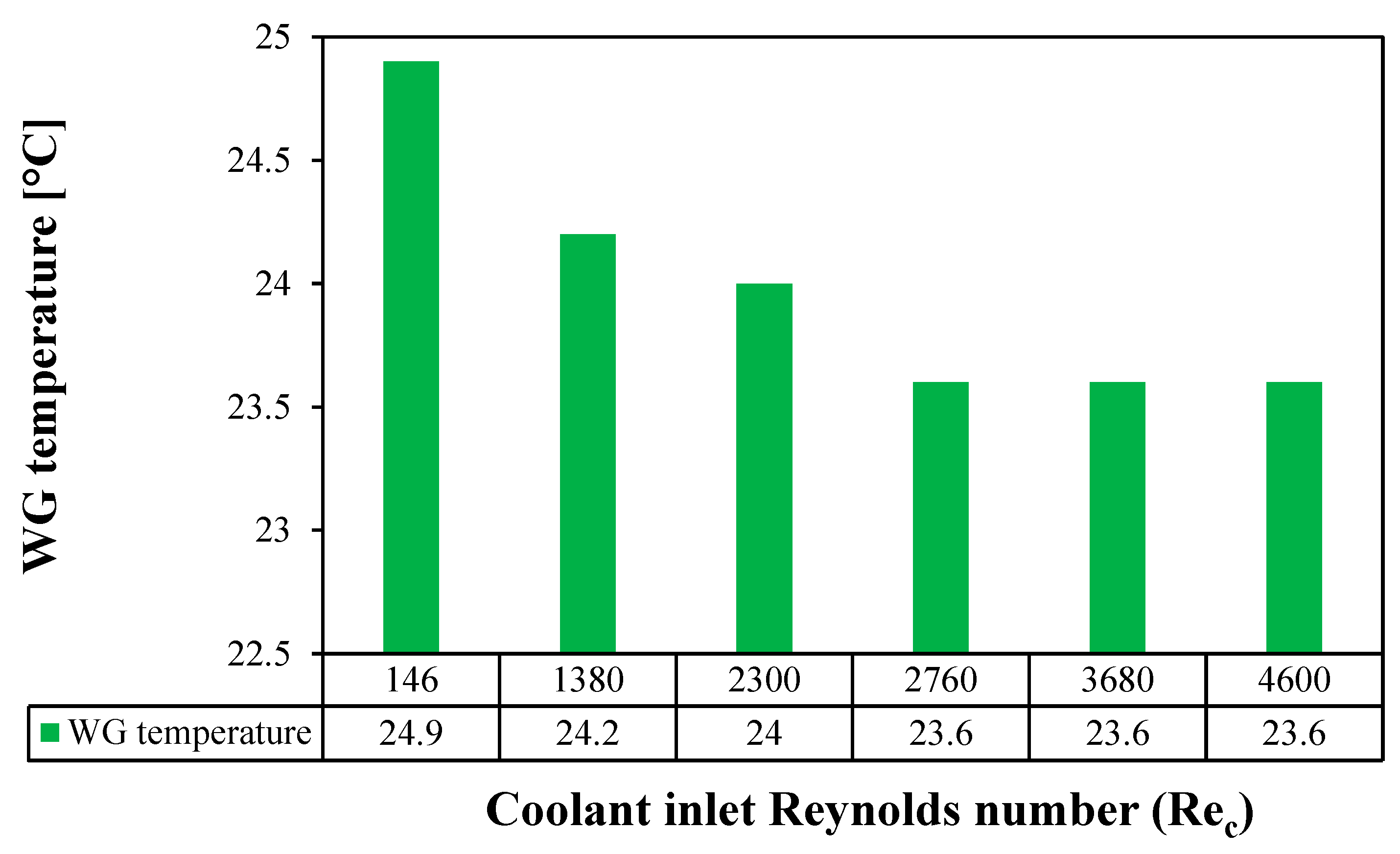
Figure 9.
Temperature distribution of WG through the circulating HF-WGMD module for different WG circulation Reynolds numbers at , and .
Figure 9.
Temperature distribution of WG through the circulating HF-WGMD module for different WG circulation Reynolds numbers at , and .
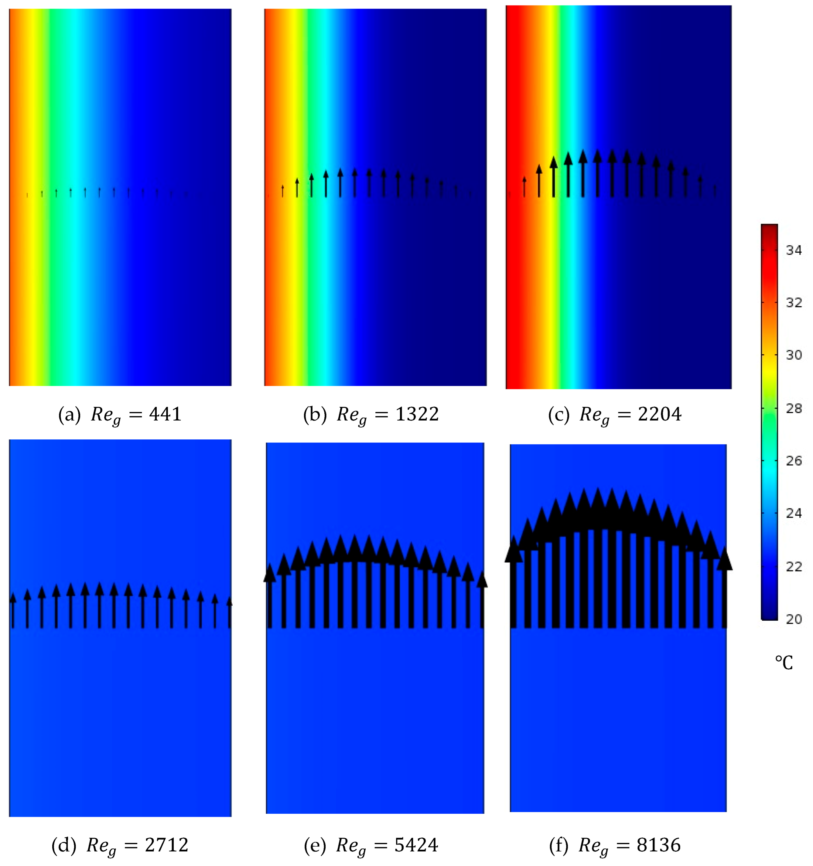
Figure 10.
Temperature distribution of membrane and WG at different feed inlet temperatures through; (a), (b), (c) and (d) stagnant and (e), (f), (g) and (h) circulating () HF-WGMD modules at and .
Figure 10.
Temperature distribution of membrane and WG at different feed inlet temperatures through; (a), (b), (c) and (d) stagnant and (e), (f), (g) and (h) circulating () HF-WGMD modules at and .
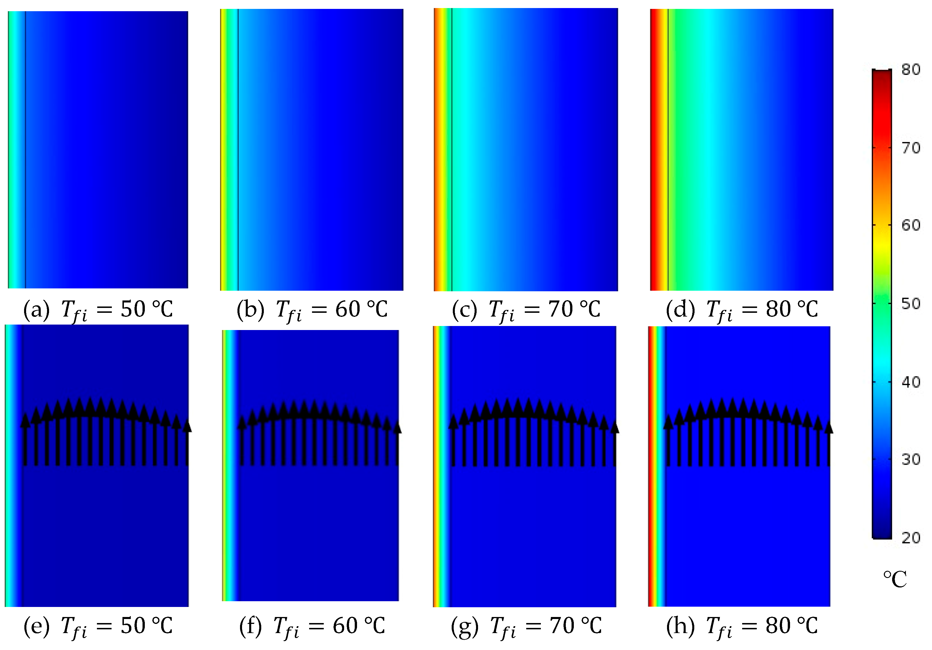
Figure 11.
Average WG temperature of the stagnant and circulating () HF-WGMD modules versus feed inlet temperature at and .
Figure 11.
Average WG temperature of the stagnant and circulating () HF-WGMD modules versus feed inlet temperature at and .
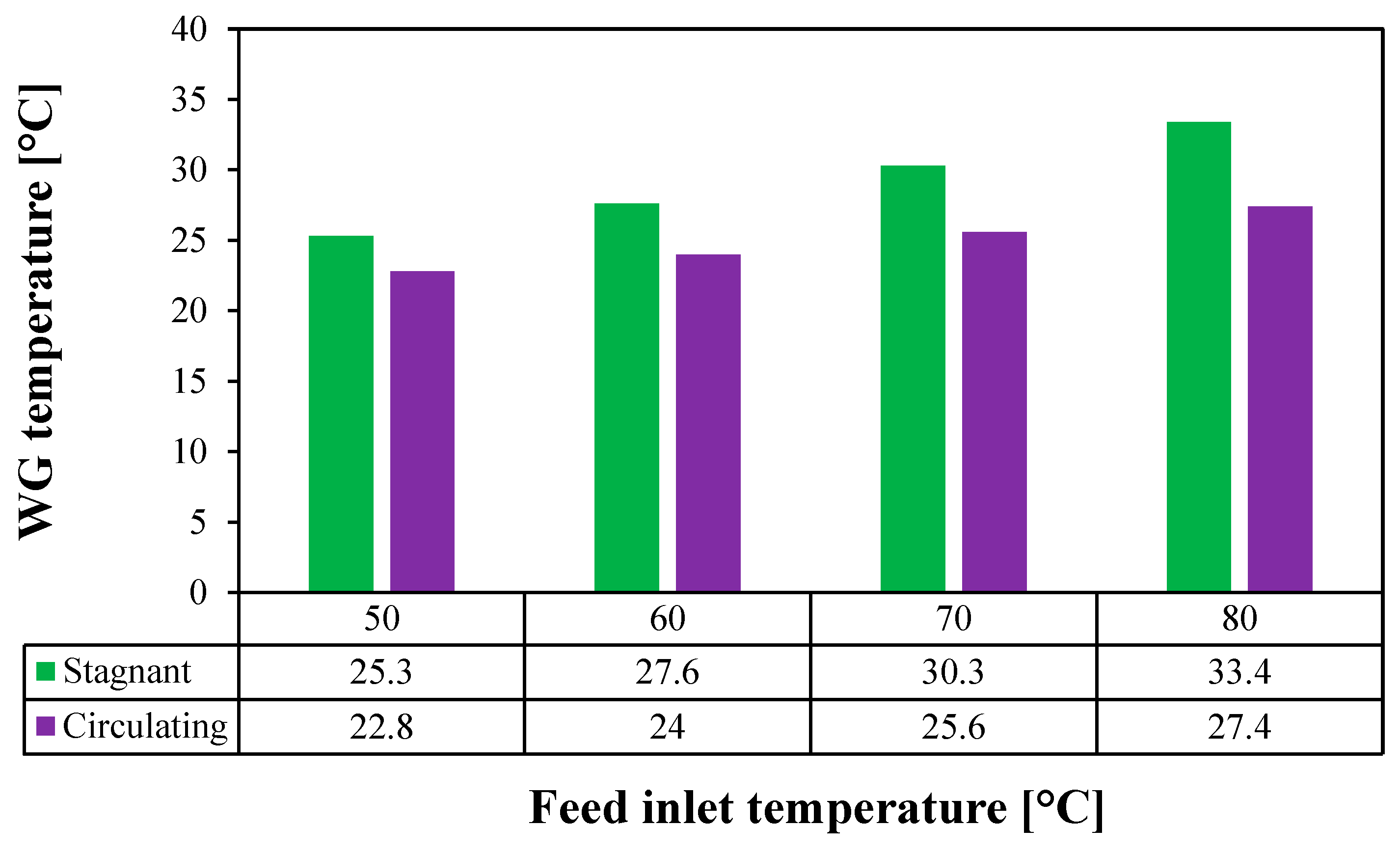
Figure 12.
Flux and feed water pressure drop for the stagnant HF-WGMD module versus feed Reynolds number at .
Figure 12.
Flux and feed water pressure drop for the stagnant HF-WGMD module versus feed Reynolds number at .
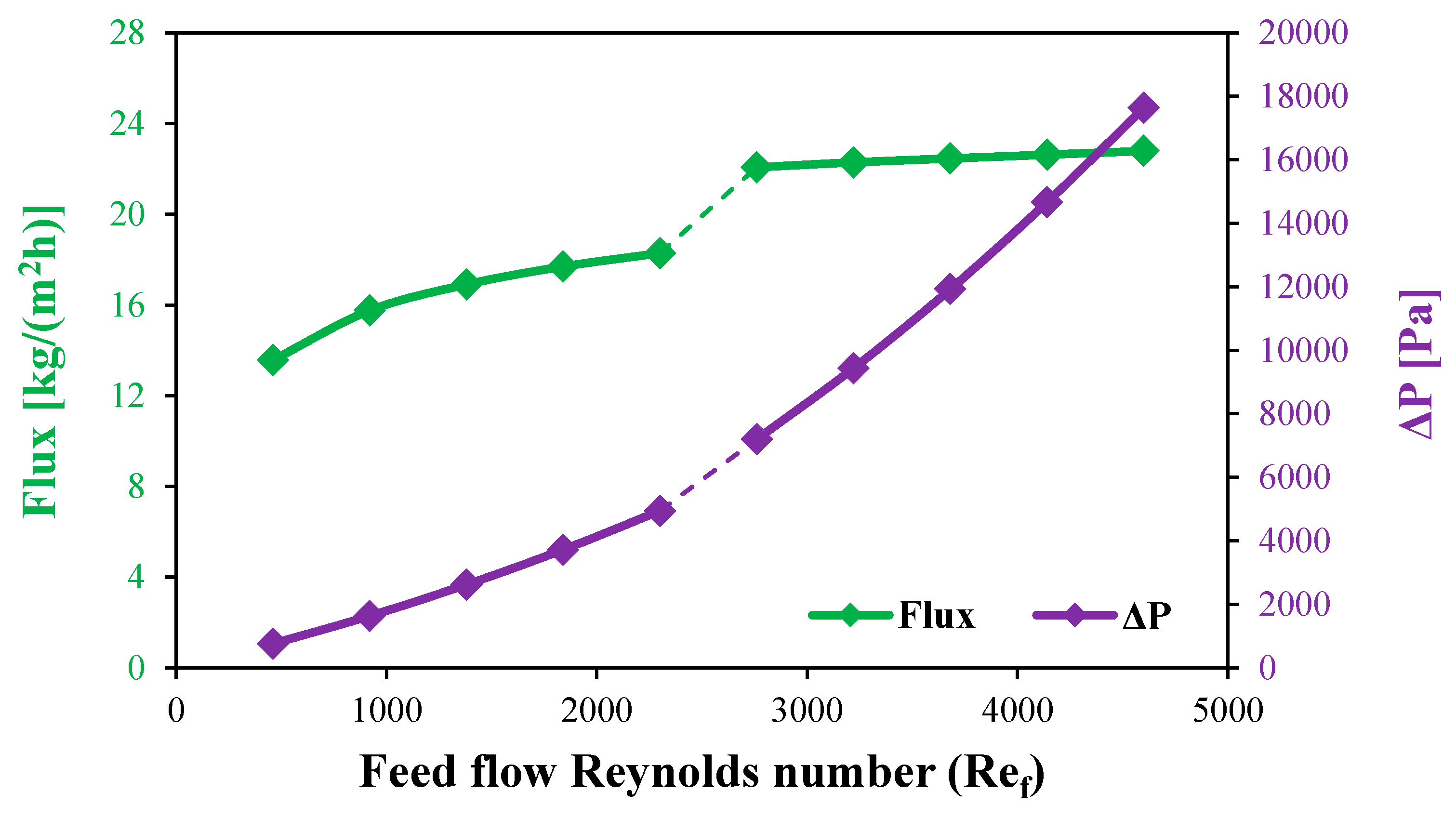
Figure 13.
Flux and cooling water pressure drop for the stagnant HF-WGMD module versus coolant Reynolds number at .
Figure 13.
Flux and cooling water pressure drop for the stagnant HF-WGMD module versus coolant Reynolds number at .
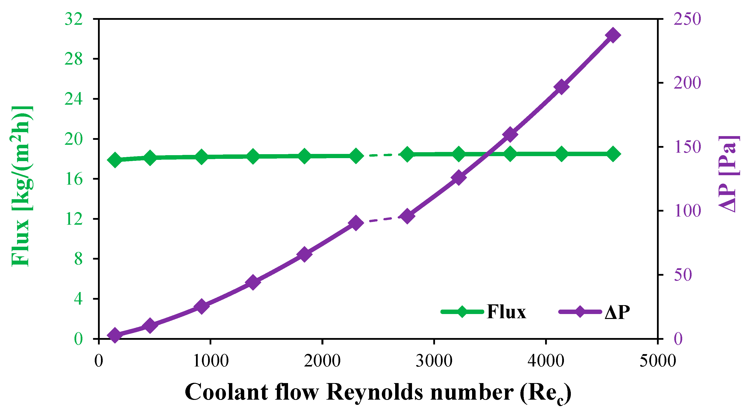
Figure 14.
Flux and WG pressure drop for the circulating HF-WGMD module versus WG circulation Reynolds number at , and different feed inlet temperatures.
Figure 14.
Flux and WG pressure drop for the circulating HF-WGMD module versus WG circulation Reynolds number at , and different feed inlet temperatures.
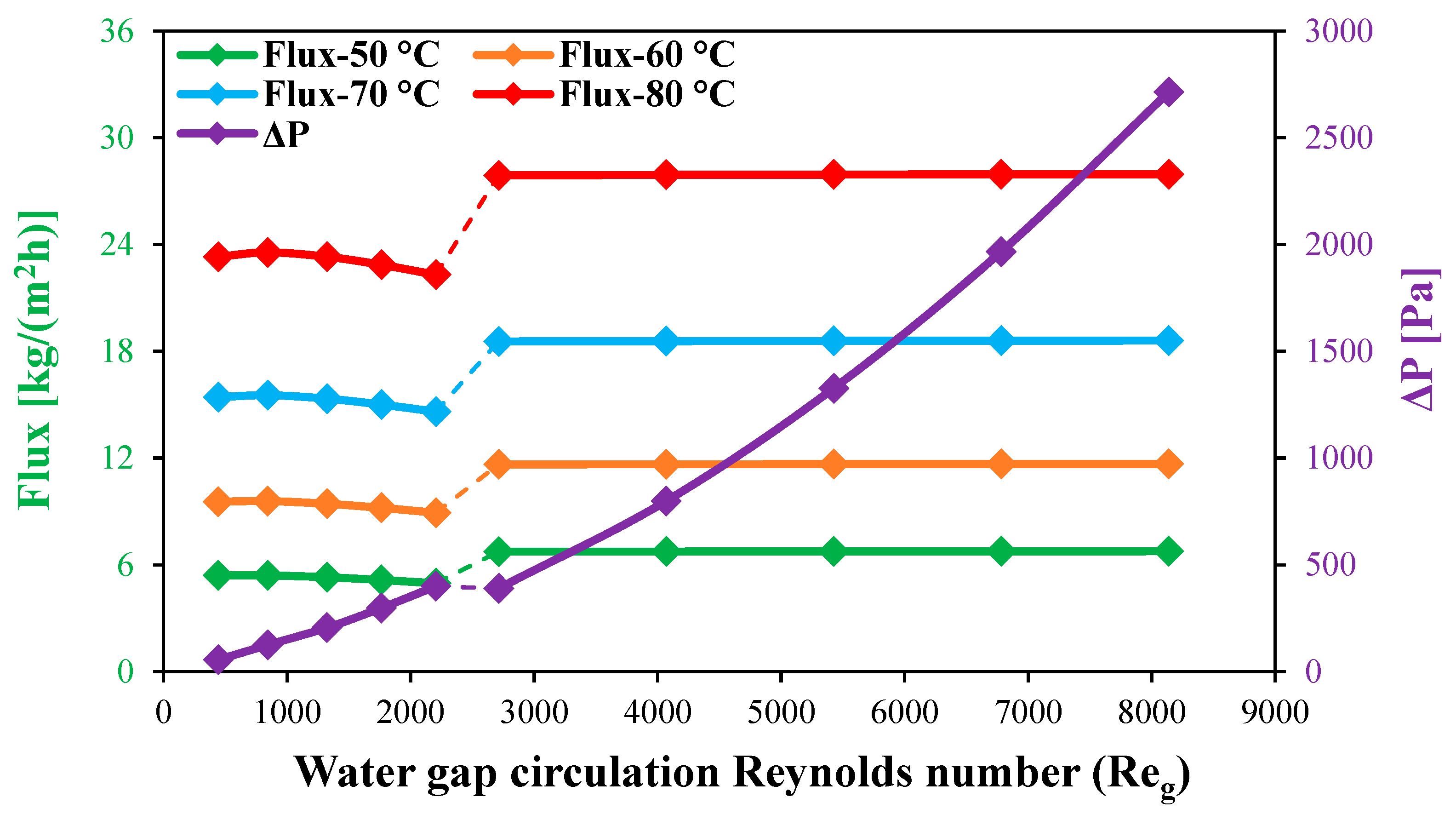
Figure 15.
Water product flux of the stagnant and circulating () HF-WGMD module versus feed inlet temperature at and .
Figure 15.
Water product flux of the stagnant and circulating () HF-WGMD module versus feed inlet temperature at and .
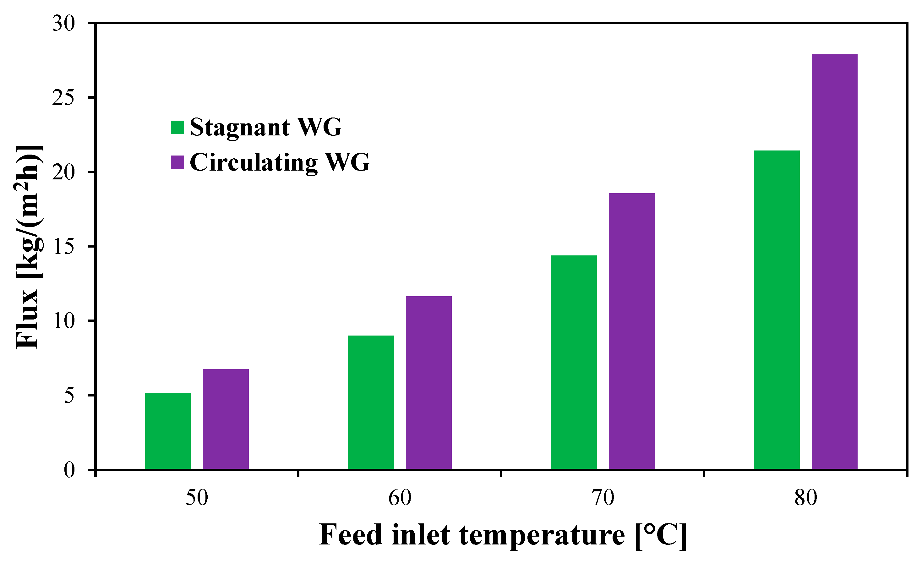
Figure 16.
The effect of the number of stages on the flux and cooling water temperature rise of MS-HF-WGMD systems at different feed inlet temperatures of (a) 50 °C, (b) 60 °C, (c) 70 °C and (d) 80 °C.
Figure 16.
The effect of the number of stages on the flux and cooling water temperature rise of MS-HF-WGMD systems at different feed inlet temperatures of (a) 50 °C, (b) 60 °C, (c) 70 °C and (d) 80 °C.
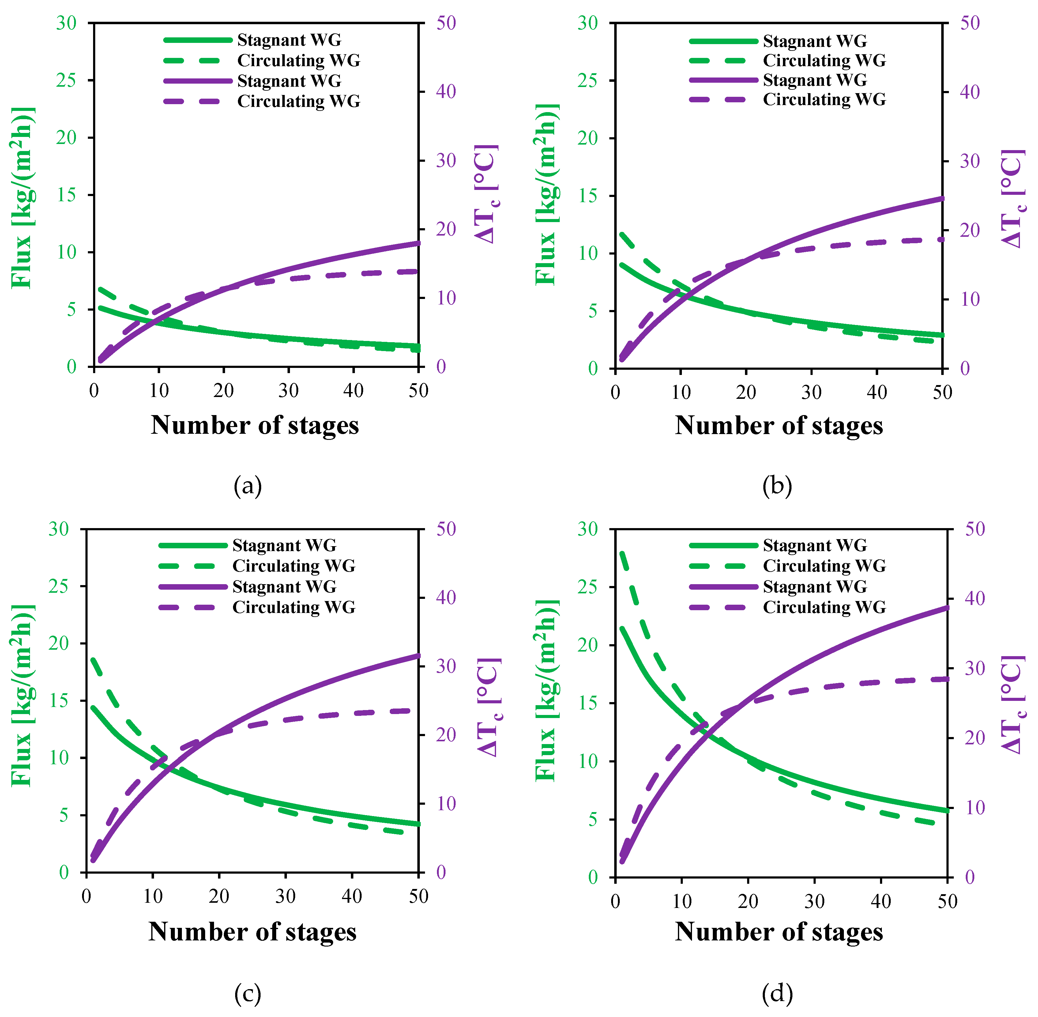
Figure 17.
The effect of the number of stages on the STEC of MS-HF-WGMD systems at different feed inlet temperatures of (a) 50 °C, (b) 60 °C, (c) 70 °C and (d) 80 °C.
Figure 17.
The effect of the number of stages on the STEC of MS-HF-WGMD systems at different feed inlet temperatures of (a) 50 °C, (b) 60 °C, (c) 70 °C and (d) 80 °C.
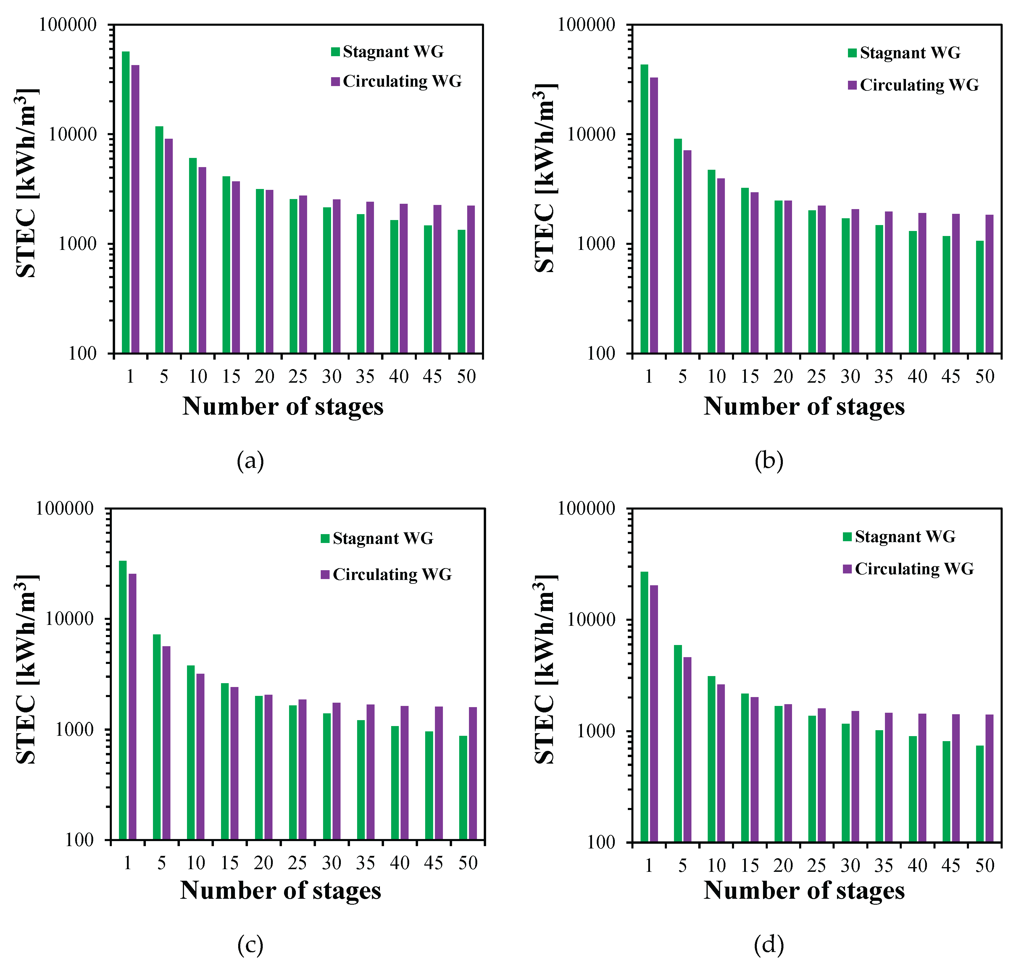

Table 1.
HF-WGMD module specifications.
| Parameter | Symbol | Value | Unit |
|---|---|---|---|
| Membrane inner radius | 0.4 | mm | |
| Membrane outer radius | 0.58 | mm | |
| Cooling tube inner radius | 2.28 | mm | |
| Cooling tube outer radius | 3.18 | mm | |
| Coolant channel radius | 2.21 | mm | |
| Module effective length | 100 | mm | |
| Feed inlet salinity | 35000 | ppm | |
| Feed water thermal conductivity | 0.64 | W/(m K) | |
| Membrane thermal conductivity | 0.07 | W/(m K) | |
| Membrane porosity | 82 | % | |
| Membrane pore tortuosity | 1.7 | - | |
| Membrane pore diameter | 0.16 | μm | |
| Water gap salinity | 0.0 | ppm | |
| Cooling tube thermal conductivity | 15 | W/(m K) | |
| Vapor molecular mass (H2O) | 18 | g/mol | |
| Salt molecular mass (NaCl) | 58.5 | g/mol |
Table 2.
Boundary conditions for the mass transport equations.
| Domain | Position | Boundary condition |
|---|---|---|
| Feed | ||
| Membrane | ||
Table 3.
Boundary conditions for the momentum transport equations.
| Domain | Position | Boundary condition |
|---|---|---|
| Feed | ||
| Circulating WG | ||
| Cooling channel | ||
Table 4.
Boundary conditions for the mass transport equations.
| Domain | Position | Boundary condition |
|---|---|---|
| Feed | ||
| Membrane | ||
| Stagnant WG | ||
| Circulating WG |
& |
Periodic |
| Cooling tube | ||
| Cooling channel | ||
Table 5.
Average temperature and concentration at feed-membrane interface of stagnant HF-WGMD module for different feed Reynolds numbers at and .
Table 5.
Average temperature and concentration at feed-membrane interface of stagnant HF-WGMD module for different feed Reynolds numbers at and .
| Feed Inlet Reynolds Numbers | ||||||
|---|---|---|---|---|---|---|
| 460 | 1380 | 2300 | 2760 | 3680 | 4600 | |
| Temperature [°C] | 45.1 | 47.2 | 47.9 | 49.5 | 49.6 | 49.7 |
| Concentration [mol/m3] | 3.53 | 3.9 | 4.04 | 4.38 | 4.42 | 4.44 |
Table 6.
Average temperature and concentration at membrane-WG interface of circulating HF-WGMD module for different WG circulation Reynolds numbers at , and .
Table 6.
Average temperature and concentration at membrane-WG interface of circulating HF-WGMD module for different WG circulation Reynolds numbers at , and .
| WG Inlet Reynolds Numbers | ||||||
|---|---|---|---|---|---|---|
| 441 | 1322 | 2204 | 2712 | 5424 | 8136 | |
| Temperature [°C] | 31.9 | 32.4 | 34.1 | 23 | 22.9 | 22.9 |
| Concentration [mol/m3] | 1.88 | 1.93 | 2.11 | 1.15 | 1.14 | 1.14 |
Disclaimer/Publisher’s Note: The statements, opinions and data contained in all publications are solely those of the individual author(s) and contributor(s) and not of MDPI and/or the editor(s). MDPI and/or the editor(s) disclaim responsibility for any injury to people or property resulting from any ideas, methods, instructions or products referred to in the content. |
© 2025 by the authors. Licensee MDPI, Basel, Switzerland. This article is an open access article distributed under the terms and conditions of the Creative Commons Attribution (CC BY) license (http://creativecommons.org/licenses/by/4.0/).
Copyright: This open access article is published under a Creative Commons CC BY 4.0 license, which permit the free download, distribution, and reuse, provided that the author and preprint are cited in any reuse.


