
Submitted:
14 July 2025
Posted:
16 July 2025
You are already at the latest version
Abstract
The K-means algorithm utilises the Euclidean distance metric to quantify the similarity between data points and clusters, with the fundamental objective of assessing the rela-tionship between points. It is important to note that, during the process of clustering, the relationships between the remaining points in the cluster and the points to be measured are ignored. In consideration of the aforementioned issues, this paper pro-poses the utilisation of the extension distance for the purpose of evaluating the rela-tionship between the points to be measured and the cluster classes. Furthermore, it in-troduces a variant of the K-means algorithm based on the separator distance. Through a series of comparative experiments, the effectiveness of the proposed algorithm for clustering fan-shaped datasets is preliminarily verified.
Keywords:
clustering
; extenics
; extension distance
1. Introduction
The K-means algorithm is regarded as a classic in the field of clustering. It employs the Euclidean distance metric to quantify the similarity between data points. The primary advantages of this approach are twofold [1]: firstly, it exhibits high computational efficiency and, secondly, it provides strong interpretability of clustering results. However, the methodology is not without its drawbacks, which include high-dimensional failure [2],susceptibility to outliers, and the tendency to form spherical clusters [3].
In order to address the aforementioned issues, scholars have proposed a number of methodologies,including PCA dimension reduction [4,5,6] and the use of Manhattan distance [7,8] or another method [9,10] to measure the similarity between data points. Although the methods proposed by scholars can effectively handle specific application scenarios [11,12,13],the clustering process of the algorithm still measures the similarity between the points to be clustered and the cluster centers, ignoring the similarity calculations between the remaining points within the cluster and the points to be clustered.
In order to address this issue, this paper proposes a variant of the K-means clustering algorithm based on the extension distance to address the aforementioned problems.
2. Extension Distance
2.1. One-Dimensional Extension Distance
In classical mathematics, distance is commonly used to measure the relationship between points and intervals.In the event that the point under consideration falls within the interval, the distance is deemed to be zero. However, it should be noted that this does not serve to differentiate between different points within the same interval. In order to differentiate between disparate points within a given interval and the interval itself, extenics [14] is introduced in the extension distance. This concept describes the positional relationship between any point and a fixed point x0 and an interval X = <a,b>. If the fixed point x0 in the internal X = <a,b> is located at the midpoint of the interval, the extension distance is:
Equation (1) delineates the relationship between point x and the interval with fixed pointx0 at the midpoint of the interval (the open or closed nature of the interval in the expandable distance is flexibly altered according to the actual situation; hence the above symbols are used to represent the interval). The subsequent illustration employs the midpoint extension distance to demonstrate its values.
As shown in Figure 1, let X be an interval. The point x of the extension distance relative to the centre of interval X = <2,4> is shown in the Figure 1. When point is outside the interval, the value of the middle extension distance is greater than zero, and the further point x is from the centre of the interval, the greater the value of .When point x inside the interval, takes its minimum value. The values of the left and right extension distances are as described in the Extenics; due to space constraints, these are not detailed here.
2.2. Limitation in High Dimensions
As mentioned above, the extension distance can accurately depict the relationship between points and intervals in one dimension. However, most datasets in the field of data analysis are high-dimensional. While applying the extension distance to analyse multiple one-dimensional datasets can leverage its advantages in describing points and intervals, this approach overlook the interdependencies between data across different dimensions. Therefore, the one-dimensional extension distance is not adequate for data analysis purposes. The concept of the kernel radius has therefore been extended to two dimensions. Feature planes are formed through the pairwise combination of all dimensions in a high-dimensional dataset and a two-dimensional kernel radius is then applied to analyse these planes. This approach retains the kernel radius’s original advantage in describing points and intervals, while mitigating the issue of neglecting inter-dimensional data correlations inherent in the one-dimensional kernel radius.
3. Extension Distance in Two-Dimensional Space
3.1. Straight Line Traversal Method
We first propose using the straight line traversal method to calculate the extension distance in two-dimensional space [15]. This method is used to calculate the extension distance between the midpoint of the plane and the set.
As shown in Figure 2a, there is a point e and a set D in a wo-dimensional plane. To calculate the extension distance between point e and set , first draw a straight line through set that passes through point e. According to the Equation (1), the extension distance between point e and the points on this line that belong to set can then be calculated:
According to Equation (2), he extension distances and of point e on the and y axes, respectively, relative to the aforementioned intervals are calculated. Equation (2) reprsents the projection of all points onto the and y axes,forming the internals and by points belonging to set D.Finally, the proportion of the extension distance corresponding to the straight line is calculated in relation to the total extension distance using the weight (where n denotes the number of points on the line belonging to the set and denotes the total number of points in set D). Note that when only one point on the line belongs to set D, all extension distance greater than zero according to Equation (1), still satisfying the property that points are outside the interval with extension distance greater than zero. As shown in Figure 2b, when all lines completely traverse the set, the extension distance of point e relative to set D can be obtained. The extension distance of set D can be calculated using the following Equation (3).
3.2. Properties and Verification
Here, and represent the weights of the extension distances in the and y directions, respectively. Their values are determined according to the actual situation.
For the purposes of illustration, consider Figure 3. Point e exhibits three distinct positional relationships with set D: the point is outside the set, the point is on the edge of the set, and the point is inside the set.
- In the event of point e lying outside set D, for any line passing through the set such that and is satisfied, it follows that for any of the above lines, and are greater than 0. Consequently, is greater than 0.The following essay will provide a comprehensive overview of the relevant literature on the subject.
- When point e is on the boundary of set D,for any line passing through the set, or ,then for any of the above lines, and are both equal to 0,so is equal to 0.
- In the event of point e being in set D,for any line passing through the set such that and ,it can be concluded that is less than 0.
In summary, upon expanding the extension distance to a two-dimensional plane, it is observed that the numerical values and meanings remain consistent with the original extension distance, as systematically categorized in Table 1.
3.3. Fixed-Angle Traversal Method
As demonstrated above, the method can be extended to a two-dimensional plane in order to describe the relationship between point and set. However, in practical applications, the line traversal method is too strict in terms of data point distribution and involves a high number of calculation steps, due to the varying distribution of data points. It is evident that the angle traversal method is further adopted to enhance calculation efficiency.As demonstrated in Figure 4, traversing the set D from a point using a fixed angle α not only reduces the requirements for data point distribution but also improves traversal computation efficiency.
3.4. Verification and Set Intersection
In light of the modification to the traversal method, it is imperative to undertake a re-verification of the extended distance calculation outcomes, ensuring their congruence with the established spatial relationships.
As shown in Figure 5a, point is located outside set . There are three possible scenarios when traversing the set at a fixed angle.
- In Scenario 1, only one point belongs to the set within the fan-shaped range. Furthermore, interval is a single point and , so we have:
- In Scenario 2: There are two or more points in the sector belonging to set and none of the sector boundaries are vertical or horizontal. According to Figure 1, we know that, for the interval so .
- In Scenario 3: There are two or more points within the sector belonging to set and a horizontal or vertical sector edge. In this case, projecting the obtained points onto the or y axis results in a single point rather than an interval, so or .According to Equation (3), analyzing the case where gives us:.
This discussion does not cover cases where one side of the sector is horizontal and the other is vertical, since the corresponding fixed angle would be too large under such conditions. Excessively large a values cause calculation errors in practical applications. In summary, when point e lies outside set , the extension distance is greater than zero if Equation (3) is used with a smaller, more reasonable fixed angle to traverse the set.
Similarly, it is straightforward to demonstrate that both points on the edge of the set (Figure 5b) and points within (Figure 5c) it satisfy the original quantitative relationship.
In summary, after changing the traversal method, the results of the extension distance calculation still maintain consistency with the position relationship. However, further verification is needed for the problem of points and multiple sets. For example, if the distance between point e and sets and is less than 0, then sets and must intersect.
To verify the above problem, assume that point E is located at the intersection of sets and . According to the preceding proof:
The simultaneous conditions in Equation (5) establish a necessary foundation for proving set intersection under negative extension distances.
Taking the x-axis as an example, sets D and F both have intervals and such that the x-coordinate of point e satisfies the following quantitative relationship:
As quantified in Equation (6), the coordinate containment relationships provide direct evidence for interval overlap on each axis dimension.
It is evident that the intervals XD and XF on the x axis overlap if they encompass the same set of points. The same applies to the y axis. Finally, It is evident that sets D and F intersect within the two-dimensional plane.
4. Kmeans Variant Based on Extension Distance
4.1. Limitations of Standard K-Means
The K-means clustering algorithm is chiefly reliant upon the utilization of the Eu-clidean distance metric to ascertain the similarity between data points. The purpose of this process is to repeatedly calculate and compare the distances between the remaining points in the dataset and the initial k centre points until the sum of these distances is minimized. The objective function is as follows [16]:
As demonstrated in the above formula, the affiliation relationship between the measured point and the cluster class is contingent on its euclidean distance to each centre point. In each calculation, the measured point is classified to the centre point with the closest distance. Subsequent to the calculation of the data set, the coordinates of each cluster class are recalculated to obtain new centre points, whereupon a new round of clustering commences. The aforementioned steps are to be repeated until the centre points stabilise. Despite the fact that the K-means algorithm is capable of rapidly and directly obtaining clustering results in a dataset, during the classification process, the algorithm solely considers the relationship between the data points and the cluster centres, disregarding the influence of other points within the cluster on the classification of the data points. Despite the utilisation of the mean coordinate calculation method in the subsequent update of the cluster centres, thereby augmenting the influence of the residual points within the cluster on the cluster centres, the fundamental process of directly determining the cluster classification of the data points remains predicated on a solitary method of point-to-point distance, a method that is encumbered by certain limitations.
4.2. Proposed Algorithm Framework
In order to address this issue, the present paper proposes a methodology based on the K-means algorithm that uses a two-dimensional extension distance to calculate the similarity between the points to be measured and the cluster classes, thereby determining the cluster class to which each point belongs.In order to calculate the similarity between the unknown points and the cluster classes, the two-dimensional extension distance method is employed to divide and traverse each cluster class in a fan shape with a fixed angle based on the unknown points. This approach ensures that the influence of each point within the cluster on the similarity of the unknown points during the classification process is comprehensively considered.In practical applications, the data sets are usually multidimensional, but the two-dimensional extension distance is limited to two-dimensional plane problems. In order to address this issue, a feature recombination method is adopted. In the context of data sets characterised by n features, these features are arranged in pairs to yield feature planes, which are subsequently calculated.Notwithstanding the fact that is substantial when the dataset under consideration contains a considerable number of features, the algorithm is required to perform calculations on multiple planes, thereby increasing the computational load. Furthermore, the method of permuting and combining features to obtain feature planes is only capable of considering the correlation between two features and is unable to analyse the intrinsic relationships among three or more features. However, even when processing datasets on a two-dimensional plane, the algorithm is able to consider the interactions between different features in multidimensional datasets, thereby partially accounting for the intrinsic relationships among features.
The following section outlines the process of the clustering algorithm based on two dimensional extension distance: [H]
1: Input: dataset , clusters n, angle
2: Calculate the distance maxima:,
3: Calculate ,,, [17]
4: for in do
5: if then
6: Set the point corresponding to as centroid
7: Break
8: end if
9: end for
10: repeat
11: Randomly select from
12: The corresponding point to
13: if all then
14: set as the centroid
15: end if
16: until Number of centres meets requirements
17: repeat
18: for in do
19: for in do
20: for in all cluster do
21: Calculate
22: end for
23:
24: belong to corresponding to min
25: end for
26: end for
27: For each cluster, find the sample corresponding to min
28:until Centre point remains stable
4.3. Angle Relation Matrix
It is imperative to note that this algorithm employs a predetermined angle α fan shape to traverse the cluster class and calculate the extension distance. In order to circumvent the repetition of calculations and enhance efficiency, it is essential to ascertain the relative angles between each point on the plane prior to calculating the extension distance on the feature plane.
As demonstrated in Figure 6, the relative angles between two points, e and h, on a plane exhibit a quantifiable relationship, as outlined below:
Therefore, for any two points in the feature plane, it is only necessary to determine the relative angle between point e and point . Then, according to Equation (8), the relative angle between point h and point e can be calculated, and finally, an relative angle square matrix can be obtained. In the context of the algorithm, the term ’relative angle’ is defined as the angle between the nth point in the data set and the first point. It has been established that there exists a quantitative relationship between the relative angle and the parameter . Consequently, the calculation of the upper or lower half of the matrix during operation is sufficient to enhance the computational efficiency of the algorithm.
The structured representation in Equation (9) achieves up to 50% storage reduction by leveraging the angular symmetry property formalized in Equation (8).
5. Algorithm Comparison Experiment
5.1. Evaluation Metrics
The evaluation of clustering effectiveness is often contingent on specific practical requirements, and there is currently a paucity of strictly unified metrics for assessing the quality of clustering results. The present study introduces two commonly used internal metrics for evaluating clustering effectiveness, namely the Davies-Bouldin Index (DBI) [18] and the Silhouette Score [19], with a view to providing a more comprehensive evaluation of clustering.Two external metrics are also considered: Adjusted Rand-Landis Index(ARI) [20] and Normalized Mutual Information(NMI) [21]. Among these, the internal metrics DBI and Silhouette Score are notable for their ability to function without the assumption of prior knowledge regarding the true distribution of clusters. Instead, the evaluation of clustering quality is based solely on the compactness within clusters and the sparsity between different clusters.
In order to verify the feasibility of the algorithm, it was compared with common clustering algorithms and the algorithm before improvement through experiments. The distribution of the data sets utilized in the experiment is illustrated in Figure 7 Each data set contains 300 sample points, which are uniformly divided into six clusters.
5.2. Datasets and Experimental Setup
In order to verify the feasibility of the algorithm, it was compared with common clustering algorithms and the algorithm before improvement through experiments. The distribution of the data sets utilised in the experiment is illustrated in Figure 7. Each data set contains 300 sample points, which are uniformly divided into six clusters.
5.3. Clustering Results Visualization
The clustering results of the algorithms for datasets A and B are shown in Figure 8. In the context of dataset A, both the enhanced algorithm and conventional clustering algorithms, such as GMM, encounter a similar predicament: they are unable to effectively differentiate between the closest points within clusters. The centre of the dataset was erroneously designated as belonging to a single cluster; however, in reality, this location is where the points from multiple clusters are most densely distributed. Due to the erroneous classification of the centre as a single cluster and the initial number of clusters being set to six, these algorithms are required to divide the remaining sample points surrounding the centre into five clusters, despite the fact that they actually belong to six clusters. The sequence of errors initiated by the erroneous categorisation of the dataset centre results in the suboptimal clustering efficacy of the aforementioned algorithms on dataset A. Despite the limitations of the proposed algorithm in this paper in fully restoring the genuine proportions of each cluster type in dataset A to a high degree, as demonstrated in Figure 8 in comparison to the true distribution of data A in Figure 7a, the cluster type proportions corresponding to the purple and cyan regions are comparatively diminutive, whilst those corresponding to the blue, green, and orange regions are comparatively substantial.Furthermore, the central segment of dataset A was originally distributed across six cluster points. However, following clustering by the algorithm, only four cluster points remained in the central segment, resulting in some cluster points being incorrectly classified in the central region of dataset A. Nevertheless, the algorithm reasonably reproduces the distribution trends of the clusters: six clusters are distributed in a fan-shaped pattern within a circular dataset.
Dataset B is a simplified version of dataset A. The six clusters are distributed in a circular dataset in a fan-shaped pattern, but in dataset B, the clusters only touch each other in the centre. There are also certain blank areas on both sides of each cluster’s fan shape. Notwithstanding this fact, the conventional clustering algorithms continue to generate the same error as with dataset A: they categorize the centre of dataset B as a solitary cluster. In a similar manner, the remaining sample points surrounding the central part of Dataset B are to be divided into five clusters by these algorithms. However, in reality, they are six clusters. It is evident that, due to the presence of blank intervals between the clusters in dataset B, the clustering errors of the algorithm are more pronounced in Figure 8. To illustrate this, the clustering results of dataset B, obtained using the improved algorithm, were analysed. It was found that the algorithm incorrectly classified the central part of dataset B into a single cluster. This resulted in a chain reaction that necessitated the division of the remaining six sector parts into five clusters. As is evident in the figure, the red clusters are distributed across three sector regions, while the purple and blue clusters are distributed across two sector regions. However, in Dataset B, it was found that each sector region corresponded to only one colour cluster. The erroneous categorisation of the central element invariably results in erroneous cluster divisions in subsequent iterations of the algorithm. Despite the enhanced algorithm’s inability to adequately segment the primary component of dataset B, the central portion, which is comprised of six distinct clusters, is successfully divided into clusters that correspond to the blue and green categories. Additionally, a segment of the green cluster exhibits a transition into the orange cluster. However, the clustering results of the proposed algorithm for dataset B demonstrate a superior reproduction of the distribution of clusters in dataset B in comparison to other algorithms, Figure 8g.
5.4. Quantitative Results Analysis
The results of evaluating the clustering performance of various algorithms on datasets A and B using two external and internal metrics are shown in Table 2 and Table 3. It is evident that, among these metrics, external metrics ARI and NMI indicate a close correlation between the proximity of their values to 1 and the extent to which the clustering results align with the true cluster distribution. The internal metric Silhouette Score indicates that the closer its value is to 1 and the closer DBI is to 0, the better the clustering: each cluster is well-defined, with tight internal cohesion and significant separation between clusters.
As demonstrated in the above tables, the proposed algorithm in this paper demonstrates superior performance in terms of external metrics when compared to other algorithms. This finding is further substantiated by the clustering results presented in Figure 8, which illustrate that, under the true distribution of the reference dataset, the proposed algorithm can effectively cluster and reproduce the true shape of the dataset, in contrast to the performance of other algorithms. However, the implementation of alternative algorithms has been observed to result in the erroneous classification of clusters within the central region of the dataset. This has been shown to precipitate a sequence of cascading reactions,resulting in a significant deviation of the clustering outcomes from the underlying true distribution of the dataset. This issue is also reflected in external metrics based on the true labels of the dataset, particularly in the ARI metric, where other algorithms perform significantly worse than the proposed algorithm. With regard to internal metrics such as the Silhouette Score and DBI, the proposed algorithm demonstrates suboptimal performance. This is particularly evident in the DBI metric, where, despite the proposed algorithm exhibiting a reduced gap in comparison to alternative algorithms, it nevertheless achieves a lower ranking. This phenomenon may be attributed to one of the limitations inherent in the DBI: It is evident that there is a deficiency in the robustness of the system with regard to non-spherical or non-circular clusters, which may result in erroneous evaluations. The clustering results of the present algorithm for datasets A and B manifest as fan-shaped, and similarly, due to the non-spherical and non-circular nature of the clusters, the present algorithm also performs poorly on the internal metric Silhouette Score. Despite the fact that the proposed algorithm performs inadequately in terms of the two internal metrics, the disparities between the algorithms in the experiments are less pronounced in the internal metrics than in the external metrics. Through experimentation on datasets A and B, the effectiveness of the proposed algorithm in handling fan-shaped distribution datasets has been verified.
6. Discussion
The present paper puts forward a variant of the K-means clustering algorithm based on the extension distance, which has been validated through comparative experiments on two datasets with fan-shaped distribution characteristics. However, further research is required to analyze the factors influencing the extension distance clustering algorithm.
Meanwhile Clustering algorithms based on two-dimensional extension distance involve the setting of two initial variables: the scanning angle and the number of clusters. Of these, the scanning angle has been demonstrated to have a significant impact on the clustering results. At this juncture, further exploration is required into the establishment of a reasonable scanning angle and the influence of the scanning angle on the clustering results.In summary, the proposed extension distance-based K-means variant successfully overcomes the spherical clustering limitation of traditional K-means by incorporating the relationships within clusters, as validated through comparative experiments on fan-shaped datasets (Figure 7 and Figure 8). This approach enhances clustering accuracy for non-spherical distributions, particularly in scenarios with high inter-cluster sparsity. However, the identified limitations, such as sensitivity to the scanning angle and non-convex set handling, warrant further investigation to broaden applicability. Overall, this work provides a robust framework for fan-shaped data clustering, with potential extensions to other non-Euclidean distance metrics in future studies.
7. Conclusions
This study introduced a novel K-means variant based on the extension distance, designed to address the limitations of traditional spherical clustering in fan-shaped data distributions. By leveraging the extension distance metric, the algorithm incorporates intra-cluster relationships, enabling more accurate clustering for non-spherical datasets, as demonstrated through rigorous experiments on benchmark fan-shaped datasets (Datasets A and B). Key findings include:
- The proposed algorithm significantly outperforms conventional methods (e.g., K-means++, GMM) in external metrics such as ARI and NMI, highlighting its robustness for fan-shaped distributions.
- The two-dimensional extension distance framework effectively handles inter-feature correlations, overcoming the high-dimensional limitations of one-dimensional approaches.
However, challenges remain in optimizing the scanning angle parameter and extending the method to non-convex sets. Future work will focus on adaptive angle selection and applications to multi-modal datasets. Overall, this research contributes a scalable and interpretable clustering framework, with implications for fields such as image segmentation and anomaly detection.
Institutional Review Board Statement
Not applicable. This study did not involve humans, animals, or clinical data.
References
- Yuan, C.; Yang, H. Research on K-value selection method of K-means clustering algorithm. J 2019, 2, 226–235. [Google Scholar] [CrossRef]
- Aggarwal, C.C.; Hinneburg, A.; Keim, D.A. On the surprising behavior of distance metrics in high dimensional space. In Proceedings of the International conference on database theory. Springer; 2001; pp. 420–434. [Google Scholar]
- Von Luxburg, U. A tutorial on spectral clustering. Statistics and computing 2007, 17, 395–416. [Google Scholar] [CrossRef]
- Ding, C.; He, X. K-means clustering via principal component analysis. In Proceedings of the Proceedings of the twenty-first international conference on Machine learning, 2004, p. 29.
- Xu, Q.; Ding, C.; Liu, J.; Luo, B. PCA-guided search for K-means. Pattern Recognition Letters 2015, 54, 50–55. [Google Scholar] [CrossRef]
- Feldman, D.; Schmidt, M.; Sohler, C. Turning big data into tiny data: Constant-size coresets for k-means, pca, and projective clustering. SIAM Journal on Computing 2020, 49, 601–657. [Google Scholar] [CrossRef]
- Suwanda, R.; Syahputra, Z.; Zamzami, E.M. Analysis of euclidean distance and manhattan distance in the K-means algorithm for variations number of centroid K. In Proceedings of the Journal of Physics: Conference Series. IOP Publishing, Vol. 1566; 2020; p. 012058. [Google Scholar]
- Wu, Z.; Song, T.; Zhang, Y. Quantum k-means algorithm based on Manhattan distance. Quantum Information Processing 2022, 21, 19. [Google Scholar] [CrossRef]
- Singh, A.; Yadav, A.; Rana, A. K-means with Three different Distance Metrics. International Journal of Computer Applications 2013, 67. [Google Scholar] [CrossRef]
- Faisal, M.; Zamzami, E.; et al. Comparative analysis of inter-centroid K-Means performance using euclidean distance, Canberra distance and manhattan distance. In Proceedings of the Journal of Physics: Conference Series. IOP Publishing, Vol. 1566, 012112. 2020. [Google Scholar]
- Chen, L.; Roe, D.R.; Kochert, M.; Simmerling, C.; Miranda-Quintana, R.A. k-Means NANI: an improved clustering algorithm for Molecular Dynamics simulations. Journal of chemical theory and computation 2024, 20, 5583–5597. [Google Scholar] [CrossRef] [PubMed]
- Premkumar, M.; Sinha, G.; Ramasamy, M.D.; Sahu, S.; Subramanyam, C.B.; Sowmya, R.; Abualigah, L.; Derebew, B. Augmented weighted K-means grey wolf optimizer: An enhanced metaheuristic algorithm for data clustering problems. Scientific reports 2024, 14, 5434. [Google Scholar]
- Huang, W.; Peng, Y.; Ge, Y.; Kong, W. A new Kmeans clustering model and its generalization achieved by joint spectral embedding and rotation. PeerJ Computer Science 2021, 7, 450. [Google Scholar] [CrossRef] [PubMed]
- Cai, W. Extension theory and its application. Chinese science bulletin 1999, 44, 1538–1548. [Google Scholar] [CrossRef]
- Qin, Y.; Li, X. A method for calculating two-dimensional spatially extension distances and its clustering algorithm. Procedia Computer Science 2023, 221, 1187–1193. [Google Scholar] [CrossRef]
- Lloyd, S. Least squares quantization in PCM. IEEE transactions on information theory 1982, 28, 129–137. [Google Scholar] [CrossRef]
- Zhao, Y.; Zhu, F.; Gui, F.; Ren, S.; Xie, Z.; Xu, C. Improved k-means algorithm based on extension distance. CAAI transactions on intelligent systems 2020, 15, 344–351. 425. [Google Scholar]
- Davies, D.L.; Bouldin, D.W. A cluster separation measure. IEEE transactions on pattern analysis and machine intelligence 1979, pp. 224–227.
- Rousseeuw, P.J. Silhouettes: a graphical aid to the interpretation and validation of cluster analysis. Journal of computational and applied mathematics 1987, 20, 53–65. [Google Scholar] [CrossRef]
- Hubert, L.; Arabie, P. Comparing partitions. Journal of classification 1985, 2, 193–218. [Google Scholar] [CrossRef]
- Strehl, A.; Ghosh, J. Cluster ensembles—a knowledge reuse framework for combining multiple partitions. Journal of machine learning research 2002, 3, 583–617. [Google Scholar]
Figure 1.
Schematic Diagram of Extension Distance.
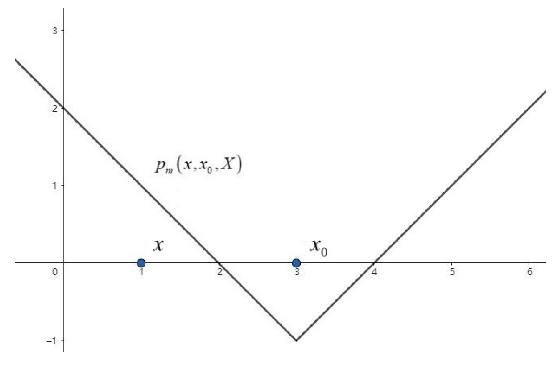
Figure 2.
(a) Schematic Diagram of Straight Line Traversal Calculation. (b) Schematic Diagram of Line Traversal Calculation Set .
Figure 2.
(a) Schematic Diagram of Straight Line Traversal Calculation. (b) Schematic Diagram of Line Traversal Calculation Set .
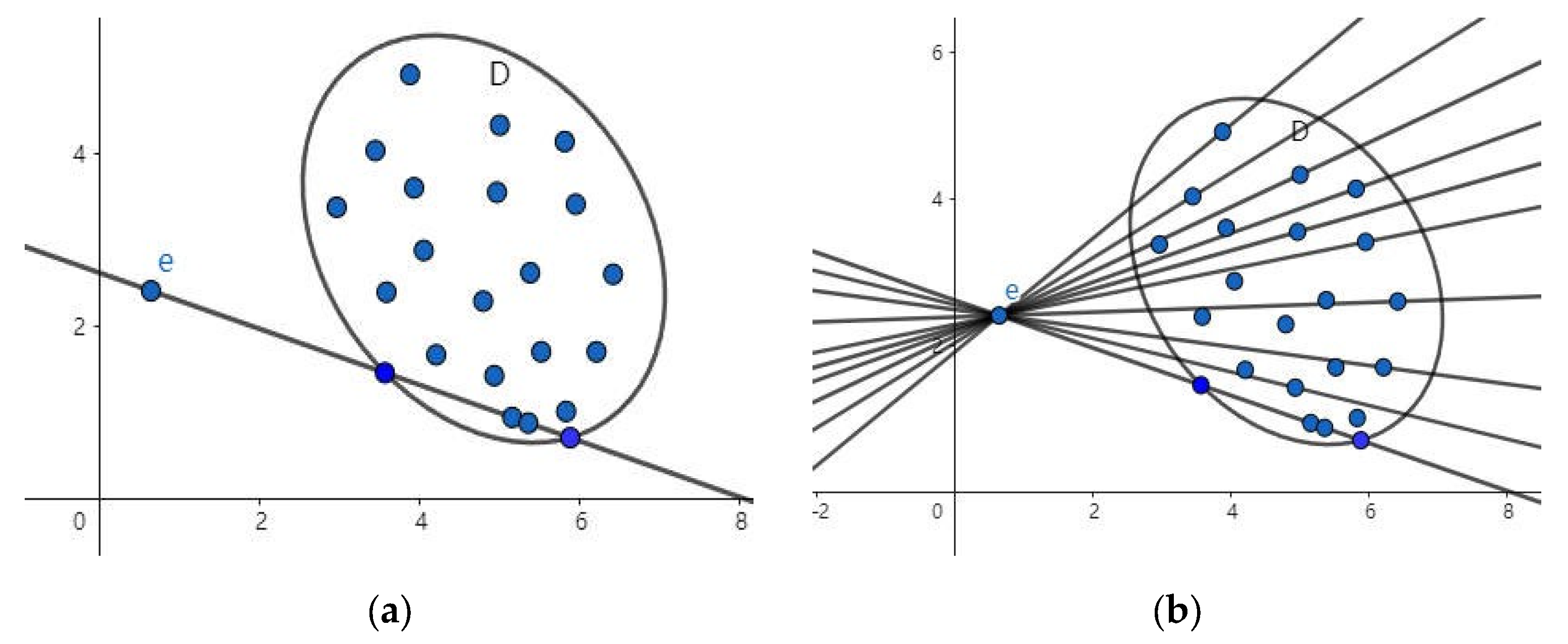
Figure 3.
(a) Point Outside the Set. (b) Point on the Edge of the Set. (c) Point Inside the Set.
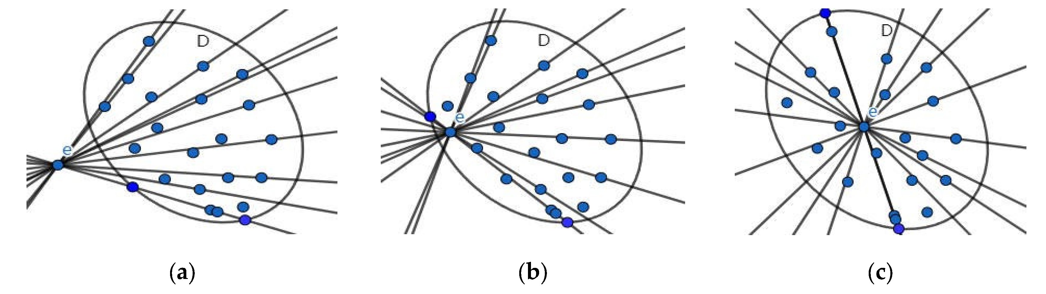
Figure 4.
Schematic Diagram of Traversing a Set at an Angle.
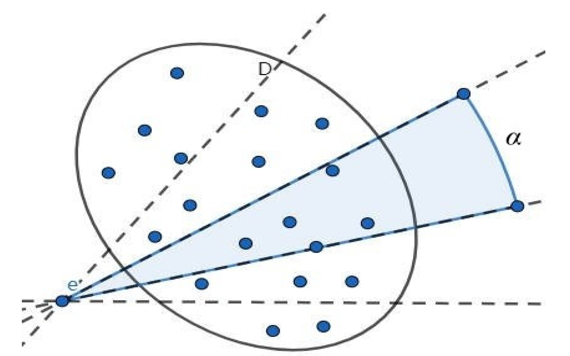
Figure 5.
(a)Point Outside the Set. (b) Point on the Edge of the Set. (c) Point Inside the Set.
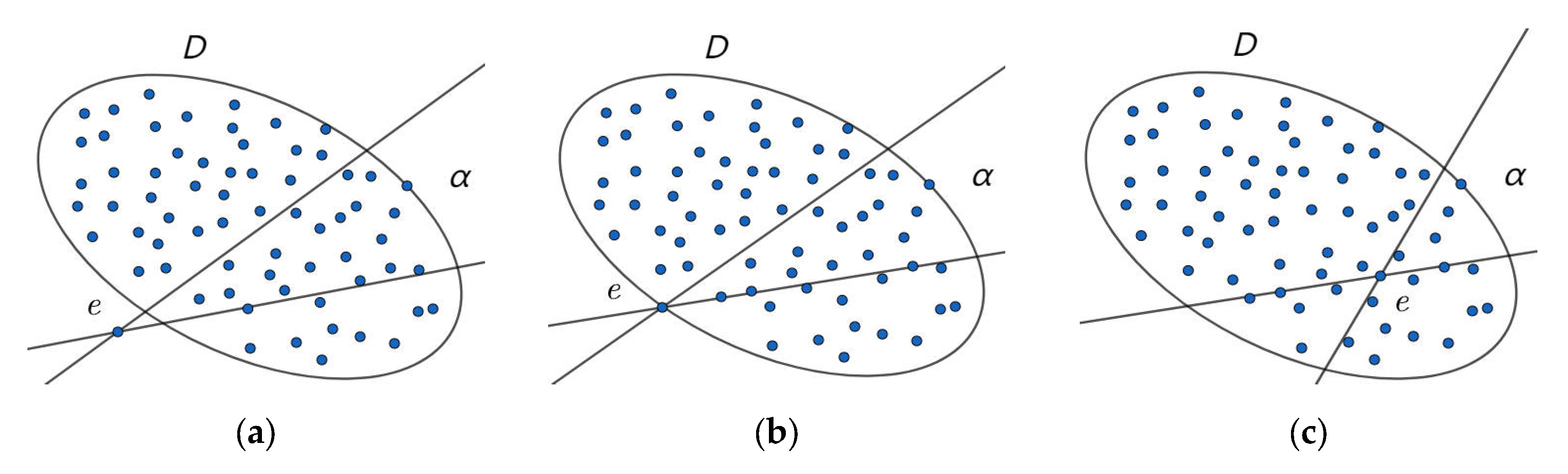
Figure 6.
(a) Relative positional relationship between points 1. (b) Relative positional relationship between points 2. (c) Relative positional relationship between points 3. (d) Relative positional relationship between points 4.
Figure 6.
(a) Relative positional relationship between points 1. (b) Relative positional relationship between points 2. (c) Relative positional relationship between points 3. (d) Relative positional relationship between points 4.
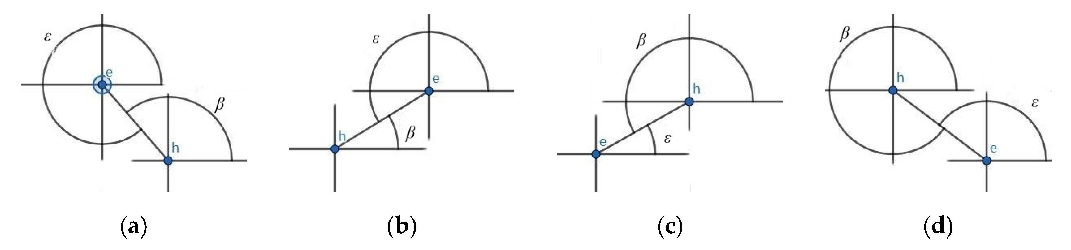
Figure 7.
(a) Dataset A. (b) Dataset B.
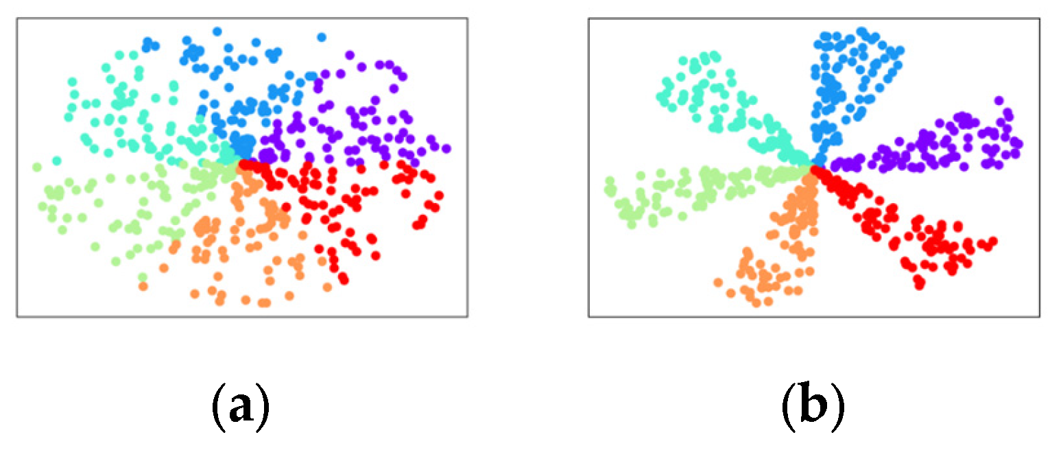
Figure 8.
(a) Results of algorithm before improvement on dataset A. (b) Results of the proposed algorithm on dataset A. (c) Results of Kmeans++ on dataset A. (d) Results of GMM on dataset A. (e)Results of Agglomerative on dataset A. (f) Results of algorithm before improvement on dataset B. (g)Results of the proposed algorithm on dataset B. (h) Results of Kmeans++ on dataset B. (i) Results of GMM on dataset B. (j) Results of Agglomerative on dataset B.
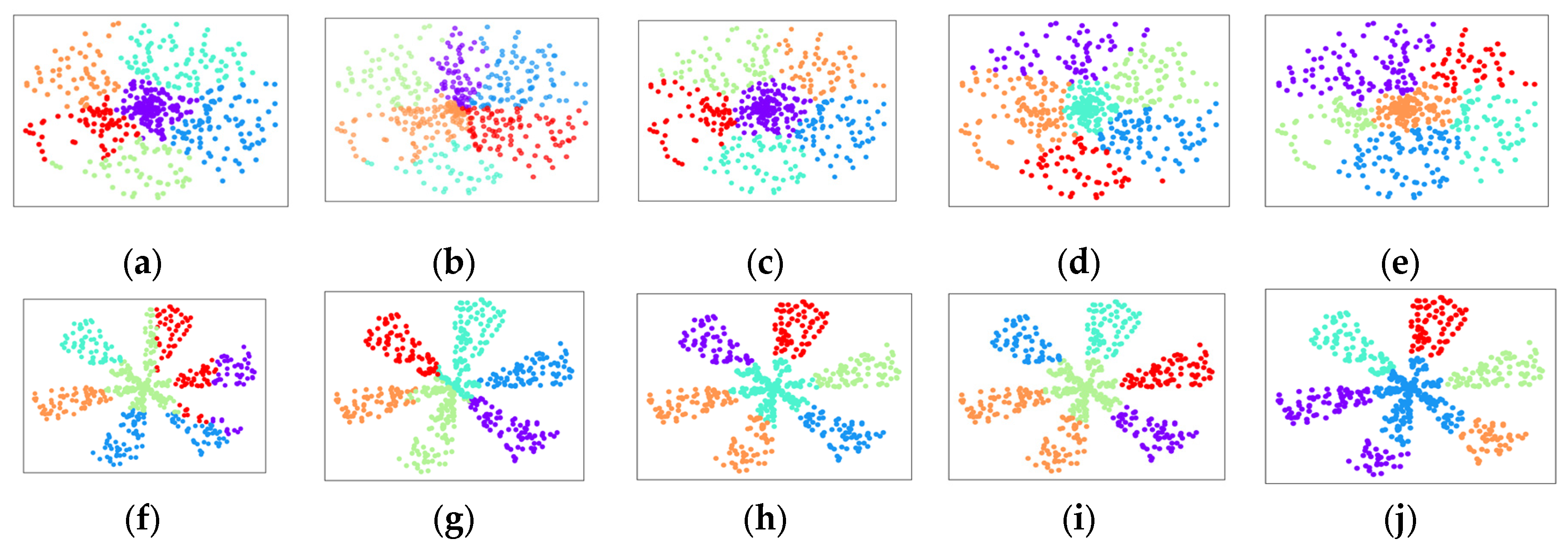

Table 1.
The extension distance between point and intervals or sets.
| The positionalrelationship betweenpoints and intervals or set | Extension distancebetween point andinterval | Extension distancebetween point andtwo-dimensional plane set |
|---|---|---|
| Point outside the interval or set |
||
| Point on the edge of the interval or set |
||
| Point inside the interval or set |
Table 2.
Dataset A Clustering Results on the Evaluation of Clustering Metrics.
| Algorithm | ARI | NMI | SilhouetteScore | DBI |
|---|---|---|---|---|
| Algorithm before Improvement |
0.304 | 0.480 | 0.329 | 0.904 |
| This article’s algorithm |
0.480 | 0.597 | 0.259 | 0.974 |
| Kmeans++ | 0.289 | 0.485 | 0.388 | 0.794 |
| GMM | 0.383 | 0.526 | 0.346 | 0.860 |
| Agglomerative | 0.305 | 0.478 | 0.330 | 0.854 |
Table 3.
Dataset B Clustering Results on the Evaluation of Clustering Metrics.
| Algorithm | ARI | NMI | SilhouetteScore | DBI |
|---|---|---|---|---|
| Algorithm before Improvement |
0.328 | 0.529 | 0.354 | 0.855 |
| This article’s algorithm |
0.658 | 0.736 | 0.367 | 0.927 |
| Kmeans++ | 0.378 | 0.604 | 0.473 | 0.732 |
| GMM | 0.389 | 0.610 | 0.471 | 0.732 |
| Agglomerative | 0.395 | 0.617 | 0.453 | 0.760 |
Disclaimer/Publisher’s Note: The statements, opinions and data contained in all publications are solely those of the individual author(s) and contributor(s) and not of MDPI and/or the editor(s). MDPI and/or the editor(s) disclaim responsibility for any injury to people or property resulting from any ideas, methods, instructions or products referred to in the content. |
© 2025 by the authors. Licensee MDPI, Basel, Switzerland. This article is an open access article distributed under the terms and conditions of the Creative Commons Attribution (CC BY) license (http://creativecommons.org/licenses/by/4.0/).
Copyright: This open access article is published under a Creative Commons CC BY 4.0 license, which permit the free download, distribution, and reuse, provided that the author and preprint are cited in any reuse.


