On the Theory of Partial Difference Equations: From Numerical Methods to Language of Complexity

1. Introduction to Partial Difference Equations

1.1. Motivation and Background

Many systems in modern biology exhibit inherently discrete organization: molecular interaction networks, cellular assemblies, and ecological populations are composed of countable entities; cells occupy spatially distinct locations; reproduction and generational turnover occur in discrete steps. Even gene expression and mutation often manifest as abrupt, stochastic events rather than smooth, continuous processes.

Nevertheless, the predominant mathematical frameworks for modeling such systems, particularly partial differential equations (PDE) are formulated in terms of continuous variables and differentiable fields [1,2]. While PDE-based models have been highly successful in physics and engineering, their reliance on smoothness and continuity can make them less well-suited for describing discrete interactions, sudden transitions, or spatially distributed logical rules that frequently arise in biological and other complex systems [3,4].

This motivates the question of whether a discrete analogue of PDE, which we term a Partial Difference Equations (P$\Delta$E), that is, a discrete-space, discrete-time equation governing the evolution of a field defined on a lattice, could serve as a more natural modeling framework for complex, emergent systems. The aim of this work is to develop a functional-analytic foundation for P$\Delta$E and to demonstrate their potential for representing systems in which local, discrete interactions give rise to large-scale collective phenomena. We propose that such a formalism offers a mathematically coherent, computationally grounded, and potentially more faithful alternative to continuous PDE in domains where discreteness is an essential feature.

1.2. Discrete Function

In this section, we introduce the concept of a discrete function, which serves as the fundamental object in our framework for discrete dynamical systems.

Definition 1 

(Discrete Function). A discrete function is a mapping

$$f:\Omega \subseteq {\mathbb{Z}}^n\to \mathbb{C},$$

where ${\mathbb{Z}}^n$ is the discrete n-dimensional integer lattice, and $\mathbb{C}$ is the codomain of the function (real, integer, or complex values depending on context).

In this paper, we primarily focus on the case where $f:{\mathbb{Z}}^n\to \mathbb{R}$, i.e., real-valued discrete functions.

Example 1 

(Discrete Single-variable Function). Let $f:\mathbb{Z}\to \mathbb{R}$ be defined as

$$f\left(x\right)=sin\left(x\right).$$

This is a real-valued function defined on the integer lattice $\mathbb{Z}$.

Example 2 

(Discrete Multivariable Function). Let $u:{\mathbb{Z}}^2\to \mathbb{Z}$ be defined as

$$u(t,x)=⌊x+sin\left(t\right)⌋.$$

Here, u maps discrete spacetime coordinates $(t,x)$ to an integer value via the floor function applied to a real expression.

1.3. Shift Operator

We define the shift operator $E^k$ acting on a discrete function $x\left(t\right)$ as

$$E^{k}x:=x(t+k)$$

for any integer $k\in \mathbb{Z}$.

Examples.

$$\begin{array}{cc}\hfill Ex& =x(t+1)\hfill \\ \hfill E^{2}x& =x(t+2)\hfill \\ \hfill E^{-1}x& =x(t-1)\hfill \end{array}$$

1.4. Partial Shift Operator

Definition. Given a discrete scalar field $u(x_1,x_2,\dots ,x_n)$, the partial shift operator $E_{x_i}^{k_i}$ acts on u by shifting the i-th coordinate:

$$E_{x_i}^{k_i}u:=u(x_1,\dots ,x_i+k_i,\dots ,x_n)$$

Examples.

$$\begin{array}{cc}\hfill E_{t}u& =u(t+1,x,y,z)\hfill \\ \hfill E_x^{2}u& =u(t,x+2,y,z)\hfill \end{array}$$

In this paper, we will write all the Partial Difference Equations in terms of Shift Operators.

1.5. Ordinary Difference Equations

Definition 2 

(Ordinary Difference Equation of Order k). An ordinary difference equation of order k is an equation involving a single-variable function $x:\mathbb{Z}\to \mathbb{C}$, expressed in terms of shift operators:

$$F(E^{n}x,E^{n-1}x,\dots ,Ex,x,E^{-1}x,\dots ,E^{-m}x,t)=0,$$

where $E^{i}x:=x(t+i)$, $n,m\in {\mathbb{Z}}^{+}$, $k=m+n$ is the total order, and F is a (possibly nonlinear) function.

Definition 3 

(Definition: Linear Ordinary Difference Equation of Order k). A linear ordinary difference equation of order kis an equation of the form:

$$a_n\left(t\right)E^{n}x+a_{n-1}\left(t\right)E^{n-1}x+\dots +a_0\left(t\right)x+a_{-1}\left(t\right)E^{-1}x+\dots +a_{-m}\left(t\right)E^{-m}x=g\left(t\right),$$

where:

• $x=x\left(t\right)$ is the unknown function defined on $\mathbb{Z}$,
• $E^{j}x:=x(t+j)$ is the shift operator,
• $a_j\left(t\right)$ are known coefficient functions,
• $g\left(t\right)$ is the known input or forcing term,
• $m,n\in \mathbb{N}$ and $k=m+n$ is the total order.

1.6. Partial Difference Equation

Definition 4 

(Partial Difference Equation). Let $u:{\mathbb{Z}}^n\to \mathbb{R}$ (or $\mathbb{C}$) be a scalar function defined on the discrete lattice. A partial difference equation (P$\Delta$E) with constant order is an equation of the form:

$$F\left({\left\{E_{x_1}^{k_1}{E}_{x_2}^{k_2}\dots E_{x_n}^{k_n}u\right\}}_{(k_1,k_2,\dots ,k_n)\in S},x_1,x_2,...,x_n\right)=0,$$

where:

• $u=u(x_1,x_2,...,x_n)$
• F is a given function, which may be linear or nonlinear;
• $E_{x_i}$ denotes the shift operator in the $x_i$ direction, defined by

  $$E_{x_i}^{k_i}u=u(x_1,x_2,\dots ,x_i+k_i,\dots ,x_n);$$
• $S\subset {\mathbb{Z}}^n$ is a finite index set determining the set of applied shifts.

1.7. The Order of a Partial Difference Equation

We propose two types of order to classify the structure of partial difference equations with constant order: structural order and absolute order.

Definition 5 

(Structural Order of Partial Difference Equation). Let $u=u(x_1,x_2,\dots ,x_n)$ be a scalar function defined on a discrete lattice. A partial difference equation is of the form

$$F\left({\left\{E_{x_1}^{k_1}{E}_{x_2}^{k_2}\dots E_{x_n}^{k_n}u\right\}}_{(k_1,k_2,\dots ,k_n)\in S},x_1,x_2,...,x_n\right)=0,$$

where $S\subset {\mathbb{Z}}^n$ is a finite index set of shifts.

For each variable $x_i$, define

$$ord\left(x_i\right)=max\left(k_i\right)-min\left(k_i\right),$$

where $max\left(k_i\right)$ is the maximum order of the shift operator in $x_i$ direction, $min\left(k_i\right)$ is the minimum order of the shift operator in $x_i$ direction, and $ord\left(x_i\right)$ is the structural order in $x_i$ direction.

Then, the structural order of the equation is defined as

$$max\left(ord\left(x_1\right),ord\left(x_2\right),\dots ,ord\left(x_n\right)\right).$$

Definition 6 

(Absolute Order of Partial Difference Equation). Let $u=u(x_1,x_2,\dots ,x_n)$ and consider a partial difference equation of the form

$$F\left({\left\{E_{x_1}^{k_1}{E}_{x_2}^{k_2}\dots E_{x_n}^{k_n}u\right\}}_{(k_1,k_2,\dots ,k_n)\in S},x_1,x_2,...,x_n\right)=0,$$

where $S\subset {\mathbb{Z}}^n$ is a finite index set.

If for all $(k_1,\dots ,k_n)\in S$, the sum

$$|k_1|+|k_2|+\dots +|k_n|\le k,$$

then the equation is said to have absolute order k.

In addition:

• A shift operator $E_x^n$ is said to be of order $\left|n\right|$.
• A mixed shift operator $E_{x_1}^{k_1}{E}_{x_2}^{k_2}\dots E_{x_n}^{k_n}$ is said to be of order $|k_1|+|k_2|+\dots +|k_n|$.

1.8. Comparison with Ordinary Difference Equations

The essential difference lies in the function domain and structure:

• Ordinary Difference Equation (O$\Delta$E): Involves a single-variable function $x:\mathbb{Z}\to \mathbb{C}$, typically evolving along a one-dimensional time axis.
• Partial Difference Equation (P$\Delta$E): Involves a multi-variable function $u:{\mathbb{Z}}^n\to \mathbb{C}$, evolving over a multi-dimensional discrete lattice.
• P$\Delta$E equations utilize partial shift operators, such as $E_{x_i}$, acting independently on each coordinate axis, introducing more geometric and structural complexity.

1.9. Comparison with Partial Differential Equations

Partial difference equations can also be viewed as the discrete analogues of partial differential equations. Key distinctions include:

• Partial Differential Equations (PDE): Defined over continuous space-time domains. Dynamics are governed by partial derivatives, such as ${\displaystyle \frac{\partial u}{\partial x}}$ or ${\displaystyle \frac{{\partial }^{2}u}{\partial t^2}}$.
• Partial Difference Equations (P$\Delta$E): Defined over discrete lattice domains, where partial derivatives are replaced by partial difference operators or partial shift operators, e.g. $E_{x_i}u=u(\dots ,x_i+1,\dots )$.
• P$\Delta$E capture the dynamics of discrete systems such as cellular automata, lattice models, or numerical schemes, and often exhibit different phenomena such as intrinsic stochasticity or discrete chaos.

1.10. Advantages of Rewriting Complex Systems as Partial Difference Equations

• Elegant and Unified Framework
  Partial Difference Equations provide a universal and elegant mathematical language to describe a wide range of complex systems. Instead of relying on a fragmented set of ad hoc models, many seemingly unrelated systems can be encoded using the same formalism. This promotes unification across disciplines such as biology, physics, and computer science.
• Mathematical Rigor and Analytical Tools
  By expressing complex systems through Partial Difference Equations, we enable the use of powerful tools from modern mathematics, including functional analysis, topology, and chaos theory. This increases the precision, clarity, and theoretical strength of the analysis.
• Extending Modeling Paradigms
  Many classical models of complex systems such as Conway’s Game of Life or the sandpile model, are static in the sense that individual entities do not move, and they typically involve only a single scalar field. Reformulating these systems as Partial Difference Equations makes it straightforward to introduce multiple field coupling, or even discrete vector fields to represent additional attributes of the entities, such as phenotypic traits or movement directions. This greatly expands the range of phenomena that can be modeled within the same theoretical framework.

1.11. Scope and Limitations

In this paper, we first introduce the definition of Partial Difference Equations (P$\Delta$E) and provide a brief overview of the linear case. We then present the concepts of discrete function spaces, discrete operators, and the discrete Green’s function. Several well-known discrete models.such as cellular automata, the Abelian sandpile model, and the Ising model, will be reformulated within the P$\Delta$E framework, though without an in-depth study of each individual model.

Finally, we compare Partial Difference Equations with their continuous counterparts, Partial Differential Equations (PDE). While PDE naturally involve tools from calculus, differential geometry, and probability theory (e.g., Gaussian distributions), P$\Delta$E instead draw upon discrete calculus, combinatorics, discrete geometry, and number theory. Due to space limitations, topics such as explicit solution methods for linear equations and regularity theory of solutions are beyond the scope of this work.

Future Work.

Future investigations will address topics deliberately omitted here, such as analytical solution methods for linear P$\Delta$E, the regularity theory of solutions, and deeper exploration of specific discrete models. In particular, extending the P$\Delta$E framework to incorporate stochastic effects, irregular lattice geometries, and more general coupling topologies represents a promising direction for further research.

1.12. Classification and Examples

Partial Difference Equations (P$\Delta$E) can be categorized along several axes, including linearity, time-dependence, and dimensionality. Below are some common types:

• Linear P$\Delta$E: A P$\Delta$E is said to be linear if it is linear in u and all its shifted terms. For example:

  $$E_{t}u={\displaystyle \frac{1}{2}}(E_x^{-1}u+E_{x}u)$$
  This equation represents a discrete diffusion process, where the future state is the average of neighbouring spatial values.
• Nonlinear P$\Delta$E: Nonlinear P$\Delta$E contain nonlinear terms involving u or its shifts. For example:

  $$E_{t}u=u+sin(E_x^{-1}u-E_{x}u)$$
  Such systems can exhibit complex behaviour, including chaos and pattern formation.
• Autonomous P$\Delta$E: If the evolution rule is independent of the explicit time step t, the equation is said to be autonomous:

  $$E_{t}u=F\left({\left\{E_x^{k}u\right\}}_{k\in N}\right)$$
  These are time-invariant systems and useful for studying equilibrium dynamics.
• Non-Autonomous P$\Delta$E: If the update rule explicitly depends on t or x, the system is non-autonomous:

  $$E_{t}u=F({\left\{E_x^{k}u\right\}}_{k\in N},t,x)$$
  These equations are useful for modeling time-varying or spatially heterogeneous environments.
• System of P$\Delta$E: A coupled system of multiple interacting fields:

  $$\left\{\begin{array}{c}{E}_{t}u=f(u,E_{x}u,E_x^{-1}u,v,E_{x}v,E_x^{-1}v)\hfill \\ E_{t}v=g(u,E_{x}u,E_x^{-1}u,v,E_{x}v,E_x^{-1}v)\hfill \end{array}\right.$$
  Such systems arise in biology, physics, and complex networks.

1.13. Notations

Definition 7 

(Difference Operator). Let $x=x\left(t\right)$. The forward difference operator is defined as

$$\Delta x:=x(t+1)-x\left(t\right)$$

Definition 8 

(Partial Difference Operator). Let $u=u(t,x,y,z)$. The partial difference operator in the x-direction is defined as

$${\Delta }_{x}u:=u(t,x+1,y,z)-u(t,x,y,z)$$

Definition 9 

(Shift Operator). Let $x=x\left(t\right)$. The shift operator is defined as

$$Ex:=x(t+1)$$

Definition 10 

(Partial Shift Operator). Let $u=u(t,x,y,z)$. The partial shift operator is defined as

$$E_{x}u:=u(t,x+1,y,z)$$

Definition 11 

(Central Difference). Let $x=x\left(t\right)$. The central difference is defined as

$${\Delta }^{c}x:={\displaystyle \frac{x(t+1)-x(t-1)}{2}}$$

Definition 12 

(Partial Central Difference). Let $u=u(t,x)$. The partial central difference is defined as

$${\Delta }_x^{c}u:={\displaystyle \frac{u(t,x+1)-u(t,x-1)}{2}}$$

Definition 13 

(Backward Difference Operator). Let $x=x\left(t\right)$. The backward difference operator is defined as

$$\delta x:=x\left(t\right)-x(t-1)$$

Definition 14 

(Partial Backward Difference Operator). Let $u=u(t,x)$. The partial backward difference operator is defined as

$${\delta }_{x}u:=u(t,x)-u(t,x-1)$$

Definition 15 

(Discrete Gradient). The discrete gradient is defined as

$$\nabla :=({\Delta }_x,{\Delta }_y,{\Delta }_z)$$

Definition 16 

(Backward Gradient). The backward gradient is defined as

$${\nabla }_{\delta }:=({\delta }_x,{\delta }_y,{\delta }_z)$$

Definition 17 

(Central Gradient). The central gradient is defined as

$${\nabla }_c:=({\Delta }_x^c,{\Delta }_y^c,{\Delta }_z^c)$$

Definition 18 

(Discrete Laplacian). The discrete Laplacian is defined as

$${\nabla }^{2}u:={\nabla }_{\delta }·\nabla u={\delta }_x{\Delta }_{x}u+{\delta }_y{\Delta }_{y}u+{\delta }_z{\Delta }_{z}u$$

Definition 19 

(von Neumann neighbourhood). The von Neumann neighbourhood V is defined as the set of lattice displacements:

$$V=\left\{\right(0,1),(0,-1),(1,0),(-1,0\left)\right\}$$

Definition 20 

(Moore neighbourhood). The Moore neighbourhood M is defined as the set of lattice displacements:

$$M=\left\{\right(0,1),(0,-1),(1,0),(-1,0),(1,1),(1,-1),(-1,1),(-1,-1\left)\right\}$$

Definition 21 

(Moore Laplacian (in 2D)). The Moore Laplacian is defined as

$${\nabla }_M^{2}u:=\left(\sum _{(i,j)\in M}u(t,x+i,y+j)\right)-8u(t,x,y)$$

where M is the Moore neighbourhood excluding the center point.

Definition 22 

(Kronecker Delta Function). The Kronecker delta function $\delta \left(x\right)$ is defined as:

$$\delta \left(x\right)=\left\{\begin{array}{cc}1,\hfill & \mathit{if}x=0\hfill \\ 0,\hfill & \mathit{otherwise}\hfill \end{array}\right.$$

Definition 23 

(Heaviside Step Function). The Heaviside step function $\theta \left(x\right)$ is defined as:

$$\theta \left(x\right)=\left\{\begin{array}{cc}1,\hfill & \mathit{if}x\ge 0\hfill \\ 0,\hfill & \mathit{otherwise}\hfill \end{array}\right.$$

Definition 24 

(Signum Function). The signum function, denoted by $sign\left(x\right)$, is defined as:

$$sign\left(x\right)=\left\{\begin{array}{cc}+1\hfill & \mathit{if}x>0,\hfill \\ 0\hfill & \mathit{if}x=0,\hfill \\ -1\hfill & \mathit{if}x<0.\hfill \end{array}\right.$$

Definition 25 

(Modulo Function). The modulo function ${mod}_n\left(x\right)$ is defined as:

$${mod}_n\left(x\right)=x-n⌊{\displaystyle \frac{x}{n}}⌋$$

where $\lfloor ·\rfloor$ denotes the floor function, and $n\in \mathbb{R}$.

2. Linear Partial Difference Equations

2.1. Motivation

Although most well-known cellular automata are nonlinear partial difference equations, we believe it is inappropriate to skip the study of linear partial difference equations and proceed directly to the nonlinear case. However, due to limitations in our current capabilities, this section will be limited to introducing the formal definition of linear partial difference equations, along with three classical examples: the discrete one-dimensional transport equation, the discrete one-dimensional diffusion equation, and the discrete one-dimensional wave equation.

We will present a few particular solutions for each equation, rather than attempting to develop a general solution method.

2.2. Definition

Definition 26 

(Linear Partial Difference Equation). Let $u=u(x_1,x_2,\dots ,x_n)$ be a scalar function defined on the discrete lattice ${\mathbb{Z}}^n$. A linear partial difference equation is an equation of the form

$$\sum _{\begin{array}{c}(k_1,\dots ,k_n)\in S\end{array}}{a}_{k_1{k}_2\dots k_n}(x_1,x_2,\dots ,x_n)E_{x_1}^{k_1}{E}_{x_2}^{k_2}\dots E_{x_n}^{k_n}u(x_1,x_2,\dots ,x_n)=f(x_1,x_2,\dots ,x_n),$$

where:

• $S\subset {\mathbb{Z}}^n$ is a finite index set,
• $E_{x_i}$ is the shift operator in the $x_i$ direction: $E_{x_i}u(\dots ,x_i,\dots )=u(\dots ,x_i+1,\dots )$,
• $a_{k_1{k}_2\dots k_n}$ and f are known functions on ${\mathbb{Z}}^n$.

Definition 27 

(Linear Partial Difference Equation of Absolute Order k). Let $u=u(x_1,x_2,\dots ,x_n)$ be a scalar function on a discrete lattice ${\mathbb{Z}}^n$. A linear partial difference equation of absolute order k is an equation of the form:

$$\sum _{\begin{array}{c}|k_1|+\dots +|k_n|\le k\end{array}}{a}_{k_1{k}_2\dots k_n}(x_1,x_2,\dots ,x_n)E_{x_1}^{k_1}{E}_{x_2}^{k_2}\dots E_{x_n}^{k_n}u=f(x_1,x_2,\dots ,x_n),$$

• $(k_1,k_2,...,k_n)\in {\mathbb{Z}}^n$.
• $E_{x_i}$ is the shift operator in the $x_i$ direction: $E_{x_i}u(\dots ,x_i,\dots )=u(\dots ,x_i+1,\dots )$,
• $a_{k_1{k}_2\dots k_n}$ and f are known functions on ${\mathbb{Z}}^n$.

2.3. Discrete 1D Transport Equation

We consider the Discrete Transport Equation:

$$E_{t}u=E_x^{k}u$$

where $u:{\mathbb{Z}}^2\to \mathbb{R}$ is defined on discrete spacetime.

Initial condition:

$$u(0,x)=f\left(x\right)$$

We impose no boundary condition.

Interpretation:

Each value is transported rigidly along a discrete path. The effective velocity is $-k$, since data moves from $x+k$ to x.

Characteristic curve:

$$x\left(t\right)=x_0-kt$$

Solution

We consider the partial difference equation

$$E_{t}u=E_x^{k}u,k\in \mathbb{Z},$$

with no boundary conditions.

Let us define a new variable:

$$\xi =x+kt,$$

and define a new function

$$v(t,\xi ):=u(t,x).$$

Then we compute the time-shift of v:

$$E_{t}v=v(t+1,\xi )=v(t+1,x+k(t+1))=v(t+1,x+kt+k)=v(t+1,\xi +k)=E_t{E}_{\xi }^{k}v=E_t{E}_x^{k}u$$

$$E_{t}v=E_t{E}_x^{k}u$$

$$v=E_x^{k}u$$

On the other hand, from the original equation:

$$E_{t}u=u(t+1,x)=E_x^{k}u(t,x)=u(t,x+k).$$

Substitute $u(t,x)=v(t,\xi )$, we get:

$$E_{t}u=u(t+1,x)=v(t+1,\xi )=E_{t}v.$$

And

$$E_x^{k}u=v$$

Thus,

$$E_{t}v=v,$$

or equivalently,

$$E_{t}v=v.$$

This is just an Ordinary Difference Equation.

Now we define a new function of $\xi$ only:

$$v(t,\xi )=f\left(\xi \right),$$

which solves the equation since

$$E_{t}v=v.$$

Therefore, the general solution is

$$v(t,\xi )=f\left(\xi \right)=f(x+kt),$$

so that

$$u(t,x)=f(x+kt),$$

where $f\left(x\right)=u(0,x)$ is the initial condition.

Conclusion: The solution of the partial difference equation

$$E_{t}u=E_x^{k}u$$

is given by

$$u(t,x)=f(x+kt),$$

where f is the initial profile of u at time $t=0$.

A General Form of Discrete 1D Linear Transport Equation

$$E_{t}u=p(t,x)E_x^{k(t,x)}u+q(t,x)u+g(t,x)$$

The operator $E_x^{k(t,x)}$ is linear because it does not depend on the function u. Although this may seem counterintuitive at first, we can rigorously verify its linearity:

$$E_x^{k(t,x)}(au+bv)=au(t,x+k(t,x))+bv(t,x+k(t,x))=a{E}_x^{k(t,x)}u+b{E}_x^{k(t,x)}v$$

Thus, $E_x^{k(t,x)}$ is a linear operator.

Furthermore, we observe that the order of a difference operator does not necessarily need to be a constant; it can also be a function. To avoid confusion, we refer to the classical case where the order is constant as difference equations with constant order. When the order is a function, we refer to them as difference equations with variable order. This is a type of Functional Partial Difference Equations. In this paper, we will only discuss about Partial Difference Equations with constant order.

Unless otherwise specified, the term "difference equation" typically assumes constant order by default.

2.4. Discrete 1D Diffusion Equation

In this section, we propose a discrete analogue of the classical one-dimensional diffusion equation. The equation is given by

$${\Delta }_{t}u=\alpha {\nabla }^{2}u,$$

where

$$u=u(t,x),u:{\mathbb{Z}}^2\to \mathbb{R},$$

$${\Delta }_{t}u:=E_{t}u-u,$$

$${\nabla }^{2}u:=E_{x}u+E_x^{-1}u-2u,$$

and $\alpha \in \mathbb{R}$ is a constant representing the diffusion coefficient.

Physical Interpretation.

This equation models the diffusion of some quantity (e.g., heat, particles, or chemical concentration) across a one-dimensional discrete lattice over discrete time steps. The Laplacian term ${\nabla }^{2}u$ captures the spatial flow of the quantity due to differences between neighbouring sites, while ${\Delta }_{t}u$ describes the temporal evolution of the system.

The Discrete 1D Diffusion Equation models symmetric spreading on a 1D lattice.

Special Case

We consider the case where the diffusion coefficient $\alpha ={\displaystyle \frac{1}{2}}$. Then the equation becomes the discrete heat equation:

$$E_{t}u={\displaystyle \frac{1}{2}}\left(E_{x}u+E_x^{-1}u\right).$$

We first consider the initial condition:

$$u(0,x)=\delta \left(x\right),$$

with no boundary condition.

Then the solution is given by the discrete heat kernel:

$$u(t,x)=\delta \left({mod}_2(x+t)\right)C\left(t,{\displaystyle \frac{x+t}{2}}\right){\left({\displaystyle \frac{1}{2}}\right)}^t,$$

where the binomial coefficient $C(x,y)$ is defined as:

$$C(x,y)=\left\{\begin{array}{cc}{\displaystyle \frac{x!}{(x-y)!y!},}\hfill & \mathrm{if}0\le y\le x,\hfill \\ 0,\hfill & \mathrm{otherwise},\hfill \end{array}\right.\mathrm{with}C:{\mathbb{Z}}^2\to \mathbb{Z}.$$

We omit the proof since this solution is well known as the discrete heat kernel, or Green’s function for the discrete heat equation.

If the initial condition is instead:

$$u(0,x)=f\left(x\right),$$

with no boundary condition, then the solution is given by:

$$u(t,x)=\sum _{s\in \mathbb{Z}}f\left(s\right)\delta \left({mod}_2(x-s+t)\right)C\left(t,{\displaystyle \frac{x-s+t}{2}}\right){\left({\displaystyle \frac{1}{2}}\right)}^t.$$

Here, ${mod}_2\left(x\right):=x-2⌊{\displaystyle \frac{x}{2}}⌋$ is the modulo function.

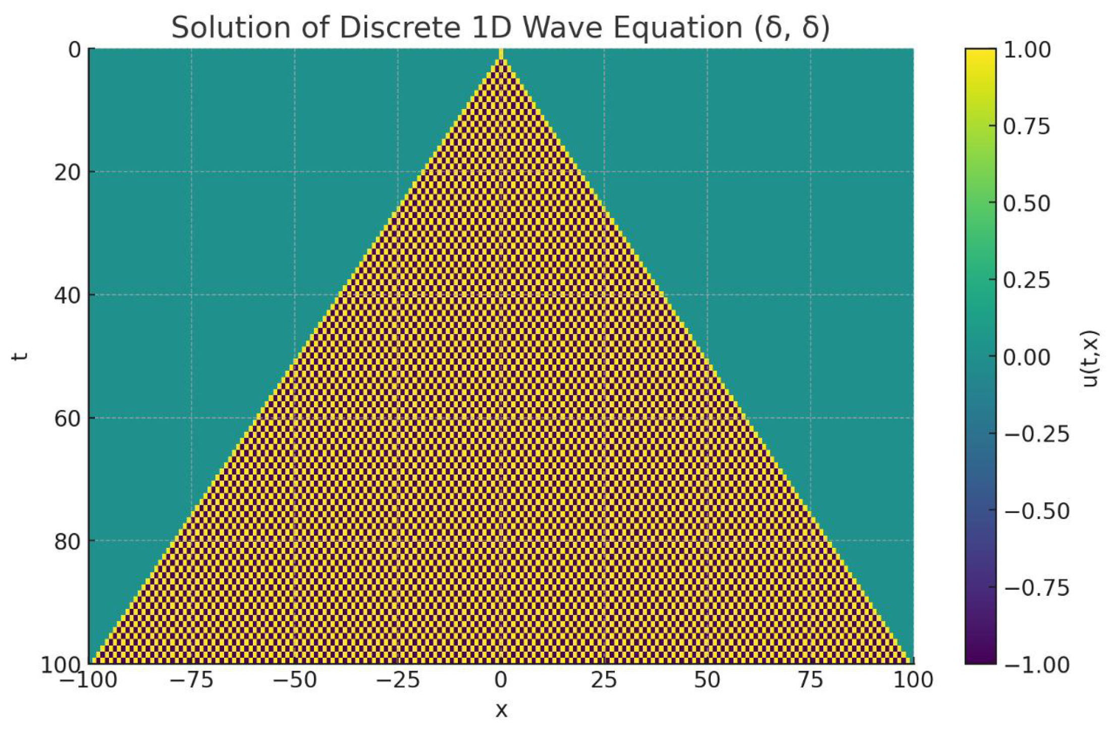
2.5. Discrete 1D Wave Equation

We define the discrete 1D wave equation as

$${\delta }_t{\Delta }_{t}u=c^2{\nabla }^{2}u$$

where $u=u(t,x)$, with $u:{\mathbb{Z}}^2\to \mathbb{R}$, and the operators are defined via shift operators:

$$\begin{array}{cc}\hfill {\delta }_t{\Delta }_{t}u& =E_{t}u+E_t^{-1}u-2u,\hfill \\ \hfill {\delta }_{t}u& =u-E_t^{-1}u(\mathrm{backward}\mathrm{difference}),\hfill \\ \hfill {\nabla }^{2}u& =E_{x}u+E_x^{-1}u-2u(\mathrm{discrete}\mathrm{Laplacian}).\hfill \end{array}$$

Physical Interpretation. This equation models a system of coupled oscillators arranged on a one-dimensional lattice. Each oscillator interacts with its nearest neighbours, and the term ${\nabla }^{2}u$ represents the net restoring force. The parameter c is a constant that governs the wave propagation speed in the discrete medium.

Special Case

We consider the case where $c=1$. Then the equation becomes:

$$E_{t}u=E_x^{-1}u+E_{x}u-E_t^{-1}u$$

with initial conditions:

$$u(0,x)=\delta \left(x\right),u(1,x)=\delta \left(x\right)$$

and no boundary condition (i.e., defined on the full lattice $\mathbb{Z}$).

Exact Solution:

$$u(t,x)=\delta \left(t\right)\delta \left(x\right)+\theta (t-1){(-1)}^{\left|x\right|+t-1}·\mathrm{com}(x,t-1)$$

where $\mathrm{com}(x,t)$ is a compact support indicator function defined by:

$$\mathrm{com}(x,a):=\left\{\begin{array}{cc}1,\hfill & \mathrm{if}\left|x\right|\le a\hfill \\ 0,\hfill & \mathrm{otherwise}\hfill \end{array}\right.$$

This can be generalized to be centered at an arbitrary point $x_0$:

$$\mathrm{com}(x-x_0,a):=\left\{\begin{array}{cc}1,\hfill & \mathrm{if}|x-x_0|\le a\hfill \\ 0,\hfill & \mathrm{otherwise}\hfill \end{array}\right.$$

The alternating sign ${(-1)}^{\left|x\right|+t-1}$ introduces a checkerboard-like structure in the wave propagation, while the compact support ensures finite spread with speed 1.

The following picture is the spatiotemporal plot of the Discrete 1D Wave Equation.

Figure 1. Spatiotemporal plot of the 1D Wave Equation

Figure 1. Spatiotemporal plot of the 1D Wave Equation

3. Discrete Function Spaces and Operators

3.1. Motivation

This section lays the theoretical foundation for the analysis of partial difference equations (P$\Delta$E). We systematically introduce the structure and properties of discrete function spaces, difference and shift operators, discrete analogues of Hilbert spaces, the Kronecker delta function, discrete Green’s functions, and boundary value problems.

The notation and operator definitions adopted here largely follow established conventions in the literature (see, e.g., [5]). The formulation and conceptual framework are inspired by the classical theory of partial differential equations (see, e.g., [6]), with appropriate adaptations to the discrete setting.

This section provides a rigorous functional-analytic formulation of shift operators. Readers primarily interested in applications may proceed directly to Section 4.

3.2. Discrete Function Spaces

Definition 28 

(Discrete Function Space). Let $\Omega \subseteq {\mathbb{Z}}^n$ be a discrete domain. We define the discrete function space over Ω as

$$F(\Omega ):=\left\{f:\Omega \to \mathbb{C}\right\},$$

i.e., the set of all functions from Ω to the complex numbers.

Definition 29 

(Discrete ${\mathcal{L}}^p$ Space). Let $\Omega \subseteq {\mathbb{Z}}^n$. We define the discrete ${\mathcal{L}}^p$ space for $1\le p<\infty$ as

$${\mathcal{L}}^p(\Omega ):=\left\{f:\Omega \to \mathbb{C}|\sum _{\mathbf{x}\in \Omega }{\left|f\left(\mathbf{x}\right)\right|}^p<\infty \right\},$$

with the corresponding ${\mathcal{L}}^p$ norm defined by

$${\parallel f\parallel }_p:={\left(\sum _{\mathbf{x}\in \Omega }{\left|f\left(\mathbf{x}\right)\right|}^p\right)}^{1/p}.$$

For $p=\infty$, we define

$${\mathcal{L}}^{\infty }(\Omega ):=\left\{f:\Omega \to \mathbb{C}|\underset{\mathbf{x}\in \Omega }{sup}\left|f\left(\mathbf{x}\right)\right|<\infty \right\},$$

with the corresponding ${\mathcal{L}}^{\infty }$ norm given by

$${\parallel f\parallel }_{\infty }:=\underset{\mathbf{x}\in \Omega }{sup}\left|f\left(\mathbf{x}\right)\right|.$$

Definition 30 

(Discrete Hilbert Space). Let $\Omega \subseteq {\mathbb{Z}}^n$. The discrete Hilbert space is the space ${\mathcal{L}}^2(\Omega )$ defined as

$${\mathcal{L}}^2(\Omega ):=\left\{f:\Omega \to \mathbb{C}|\sum _{\mathbf{x}\in \Omega }{\left|f\left(\mathbf{x}\right)\right|}^2<\infty \right\},$$

equipped with the inner product

$$\langle f,g\rangle :=\sum _{\mathbf{x}\in \Omega }f\left(\mathbf{x}\right)\overline{g\left(\mathbf{x}\right)},\mathit{for}\mathit{all}f,g\in {\mathcal{L}}^2(\Omega ).$$

This inner product satisfies the following properties for all $f,g,h\in {\mathcal{L}}^2(\Omega )$ and all scalars $\alpha \in \mathbb{C}$:

• Conjugate Symmetry:

  $$\langle f,g\rangle =\overline{\langle g,f\rangle }.$$
• Linearity in the First Argument:

  $$\langle \alpha f+h,g\rangle =\alpha \langle f,g\rangle +\langle h,g\rangle .$$
• Positive Definiteness:

  $$\langle f,f\rangle \ge 0,\mathrm{and}\langle f,f\rangle =0\iff f=0.$$

The norm induced by this inner product is

$${\parallel f\parallel }_2:=\sqrt{\langle f,f\rangle }={\left(\sum _{\mathbf{x}\in \Omega }{\left|f\left(\mathbf{x}\right)\right|}^2\right)}^{1/2}.$$

Moreover, ${\mathcal{L}}^2(\Omega )$ is complete with respect to this norm, and hence forms a Hilbert space.

3.3. Operators

Definition 31 

(Discrete Operator). Let $V,W$ be discrete function spaces, i.e., subspaces of $F(\Omega )$, where $\Omega \subseteq {\mathbb{Z}}^n$.

A discrete operator is a map

$$T:V\to W,$$

which assigns to each function $f\in V$ a function $Tf\in W$.

Definition 32 

(Shift Operator). Let $x:\mathbb{Z}\to \mathbb{C}$. We define the shift operator $E^k$ acting on a discrete function $x\left(t\right)$ by

$$E^{k}x:=x(t+k)$$

for any integer $k\in \mathbb{Z}$.

Definition 33 

(Partial Shift Operator). Given a discrete scalar field $u(x_1,x_2,\dots ,x_n)$, the partial shift operator $E_{x_i}^{k_i}$ acts on u by shifting the i-th coordinate:

$$E_{x_i}^{k_i}u:=u(x_1,\dots ,x_i+k_i,\dots ,x_n)$$

for any integer $k_i\in \mathbb{Z}$.

Definition 34 

(Difference Operator). Let $x:\mathbb{Z}\to \mathbb{C}$. We define the (forward) difference operator Δ by

$$\Delta x:=x(t+1)-x\left(t\right)$$

We may define the shift operator E as $Ex:=x(t+1)$, so that the difference operator can be written compactly as

$$\Delta x=Ex-x$$

Definition 35 

(Partial Difference Operator). Let $u:{\mathbb{Z}}^n\to \mathbb{C}$, and denote $u=u(x_1,x_2,\dots ,x_n)$. The partial difference operator with respect to the variable $x_i$ is defined as:

$${\Delta }_{x_i}u:=E_{x_i}u-u$$

where $E_{x_i}$ is the partial shift operator acting on the i-th coordinate:

$$E_{x_i}u:=u(x_1,\dots ,x_i+1,\dots ,x_n)$$

Definition 36 

(Backward Difference Operator). Let $x:\mathbb{Z}\to \mathbb{C}$ be a discrete function with $x=x\left(t\right)$. Then the backward difference operator is defined as

$$\delta x:=x\left(t\right)-x(t-1)=x-E^{-1}x$$

Definition 37 

(Partial Backward Difference Operator). Let

$$u:{\mathbb{Z}}^n\to \mathbb{C},u=u(x_1,x_2,\dots ,x_n)$$

Then the partial backward difference operator with respect to $x_i$ is defined as

$${\delta }_{x_i}u:=u-E_{x_i}^{-1}u$$

where $E_{x_i}^{-1}$ is the backward shift operator acting on the $x_i$-th coordinate.

Definition 38 

(Central Difference Operator). Let $x:\mathbb{Z}\to \mathbb{C}$, with $x=x\left(t\right)$. Then the central difference operator is defined as

$${\Delta }^{c}x:={\displaystyle \frac{1}{2}}\left(Ex-E^{-1}x\right)$$

where E is the forward shift operator: $Ex=x(t+1)$, and $E^{-1}x=x(t-1)$.

Definition 39 

(Partial Central Difference Operator). Let $u:{\mathbb{Z}}^n\to \mathbb{C}$, where $u=u(x_1,x_2,\dots ,x_n)$. Then the partial central difference operator with respect to $x_i$ is defined as

$${\delta }_{x_i}u:={\displaystyle \frac{1}{2}}\left(E_{x_i}u-E_{x_i}^{-1}u\right),$$

where $E_{x_i}$ is the shift operator in the $x_i$-direction, defined by

$$E_{x_i}u=u(x_1,\dots ,x_i+1,\dots ,x_n).$$

Definition 40 

(Discrete Gradient). Let $u:{\mathbb{Z}}^n\to \mathbb{C}$ be a discrete scalar function, where $u=u(x_1,x_2,\dots ,x_n)$. Then the discrete gradient of u is defined as the vector:

$$\nabla u:=\left({\Delta }_{x_1}u,{\Delta }_{x_2}u,\dots ,{\Delta }_{x_n}u\right)$$

where ${\Delta }_{x_i}$ is the forward partial difference operator defined by

$${\Delta }_{x_i}u:=u(x_1,\dots ,x_i+1,\dots ,x_n)-u(x_1,\dots ,x_i,\dots ,x_n)$$

for each $i=1,2,\dots ,n$.

Definition 41 

(Backward Gradient). Let

$$u:{\mathbb{Z}}^n\to \mathbb{C},u=u(x_1,x_2,\dots ,x_n),$$

then the backward gradient is defined as

$${\nabla }_{\delta }u=\left({\delta }_{x_1}u,{\delta }_{x_2}u,\dots ,{\delta }_{x_n}u\right),$$

where each ${\delta }_{x_i}u$ denotes the partial backward difference in the $x_i$-direction.

Definition 42 

(Central Gradient). Let

$$u:{\mathbb{Z}}^n\to \mathbb{C},u=u(x_1,x_2,\dots ,x_n),$$

be a discrete function on the n-dimensional integer lattice. Then the Central Gradient is defined as the vector

$${\nabla }_{c}u:=\left({\Delta }_{x_1}^{c}u,{\Delta }_{x_2}^{c}u,\dots ,{\Delta }_{x_n}^{c}u\right),$$

where each ${\Delta }_{x_i}^{c}u$ denotes the partial central difference of u with respect to the variable $x_i$.

Definition 43 

(Discrete Laplacian). Let

$$u:{\mathbb{Z}}^n\to \mathbb{C},u=u(x_1,x_2,\dots ,x_n),$$

then the Discrete Laplacian is defined as

$${\nabla }^{2}u={\nabla }_{\delta }·\nabla u=\sum _{i=1}^n{\delta }_{x_i}{\Delta }_{x_i}u,$$

where $\nabla u=({\Delta }_{x_1}u,\dots ,{\Delta }_{x_n}u)$ is the discrete gradient , and ${\nabla }_{\delta }=({\delta }_{x_1},\dots ,{\delta }_{x_n})$ is the backward gradient .

Definition 44 

(Linear Operator). Let $\Omega \subseteq {\mathbb{Z}}^n$, and let

$$T:\mathcal{D}\left(T\right)\subseteq {\mathcal{L}}^2(\Omega )\to {\mathcal{L}}^2(\Omega )$$

be a map with domain $\mathcal{D}\left(T\right)$. We say that T is a linear operator if for all $u,v\in \mathcal{D}\left(T\right)$ and all scalars $\alpha ,\beta \in \mathbb{C}$, the following holds:

$$T(\alpha u+\beta v)=\alpha T\left(u\right)+\beta T\left(v\right).$$

Definition 45 

(Linear Shift Operator). Let $\Omega \subseteq {\mathbb{Z}}^n$ and $m\in \mathbb{N}$. Alinear shift operatorL of absolute order at most m is any map of the form

$$L\left(u\left(\mathbf{x}\right)\right)=\sum _{\begin{array}{c}{\parallel \alpha \parallel }_1\le m\end{array}}{a}^{\alpha }\left(\mathbf{x}\right)E^{\alpha }u\left(\mathbf{x}\right),\mathbf{x}\in \Omega ,$$

where

$${\parallel \alpha \parallel }_1:=|{\alpha }_1|+\dots +|{\alpha }_n|,E^{\alpha }u\left(\mathbf{x}\right):=u(\mathbf{x}+\alpha ),$$

and the coefficient functions $a^{\alpha }:\Omega \to \mathbb{C}$ are given. Here $E_{x_i}^k$ denotes the one–step shift in the i-th coordinate,

$$E_{x_i}^{k}u(x_1,\dots ,x_i,\dots ,x_n):=u(x_1,\dots ,x_i+k,\dots ,x_n),$$

so that $E^{\alpha }=E_{x_1}^{{\alpha }_1}\dots E_{x_n}^{{\alpha }_n}$, where $\alpha =({\alpha }_1,{\alpha }_2,...,{\alpha }_n)\in {\mathbb{Z}}^n$. We take $\mathcal{D}\left(L\right)$ to be the set of all $u\in {\mathcal{L}}^2(\Omega )$ for which the right-hand side is well-defined and belongs to ${\mathcal{L}}^2(\Omega )$.

Proposition 1. 

Let L be a linear shift operator on a function space $F(\Omega )$, where $\Omega \subseteq {\mathbb{Z}}^n$. Then the solution set of the homogeneous partial difference equation

$$L\left(u\right)=0$$

is a function subspace(which is also a vector space) of $F(\Omega )$.

Proof. 

If $u,v\in kerL$ and $\alpha ,\beta \in \mathbb{C}$, then

$$L(\alpha u+\beta v)=\alpha L\left(u\right)+\beta L\left(v\right)=0,$$

so $\alpha u+\beta v\in kerL$.    □

Definition 46 

(Adjoint Operator).

Let ${\mathcal{L}}^2(\Omega )$ be a discrete Hilbert space with inner product

$$\langle f,g\rangle :=\sum _{\mathbf{x}\in \Omega }f\left(\mathbf{x}\right)\overline{g\left(\mathbf{x}\right)}.$$

Let $T:\mathcal{D}\left(T\right)\subseteq {\mathcal{L}}^2(\Omega )\to {\mathcal{L}}^2(\Omega )$ be a linear operator.

We say that a linear operator $T^{*}:\mathcal{D}\left(T^{*}\right)\subseteq {\mathcal{L}}^2(\Omega )\to {\mathcal{L}}^2(\Omega )$ is the adjoint of T if:

$$\langle Tf,g\rangle =\langle f,T^{*}g\rangle \mathrm{for}\mathrm{all}f\in \mathcal{D}\left(T\right),g\in \mathcal{D}\left(T^{*}\right).$$

Here, $\mathcal{D}\left(T^{*}\right)$ consists of all $g\in {\mathcal{L}}^2(\Omega )$ such that the map

$$f\mapsto \langle Tf,g\rangle$$

is continuous (i.e., bounded) on $\mathcal{D}\left(T\right)$.

Example 3. 

Let $\Omega \subseteq {\mathbb{Z}}^n$ be shift-invariant under $\alpha \in {\mathbb{Z}}^n$ (e.g. $\Omega ={\mathbb{Z}}^n$, or Ω with periodic boundary conditions), and consider the Hilbert space ${\mathcal{L}}^2(\Omega )$ with inner product

$$\langle f,g\rangle :=\sum _{\mathbf{x}\in \Omega }f\left(\mathbf{x}\right)\overline{g\left(\mathbf{x}\right)}.$$

For $\alpha \in {\mathbb{Z}}^n$, define the (multi-dimensional) shift

$$\left(E^{\alpha }u\right)\left(\mathbf{x}\right):=u(\mathbf{x}+\alpha ),$$

where

$$E^{\alpha }=E_{x_1}^{{\alpha }_1}\dots E_{x_n}^{{\alpha }_n},\alpha =({\alpha }_1,\dots ,{\alpha }_n)\in {\mathbb{Z}}^n$$

is the vector representing the direction (and magnitude) of the shift.

Then for all $u,v\in {\mathcal{L}}^2(\Omega )$,

$$\begin{array}{cc}\hfill \langle E^{\alpha }u,v\rangle & =\sum _{\mathbf{x}\in \Omega }u(\mathbf{x}+\alpha )\overline{v\left(\mathbf{x}\right)}=\sum _{\mathbf{y}\in \Omega }u\left(\mathbf{y}\right)\overline{v(\mathbf{y}-\alpha )}\hfill \\ & =\langle u,E^{-\alpha }v\rangle .\hfill \end{array}$$

Hence the adjoint of the shift is the opposite shift:

$${\left(E^{\alpha }\right)}^{*}=E^{-\alpha }.$$

Definition 47 

(Unitary Operator). Let $\Omega \subseteq {\mathbb{Z}}^n$ and let

$$U:\mathcal{D}\left(U\right)\subseteq {\mathcal{L}}^2(\Omega )\to {\mathcal{L}}^2(\Omega )$$

be a linear operator with domain $\mathcal{D}\left(U\right)$. We say that U is unitary if:

$$U^{*}U=U{U}^{*}=I,$$

that is,

$$U^{*}=U^{-1},$$

where $U^{*}$ is the adjoint of U and $U^{-1}$ is the inverse operator of U. Equivalently, U is unitary if it preserves the inner product:

$$\langle Uf,Ug\rangle =\langle f,g\rangle \mathrm{for}\mathrm{all}f,g\in {\mathcal{L}}^2(\Omega ).$$

Proposition 2. 

Let $\Omega \subseteq {\mathbb{Z}}^n$ be shift-invariant under $\pm \alpha \in {\mathbb{Z}}^n$ (e.g. $\Omega ={\mathbb{Z}}^n$ or Ω with periodic boundary conditions). Consider the Hilbert space ${\mathcal{L}}^2(\Omega )$ with inner product

$$\langle f,g\rangle :=\sum _{\mathbf{x}\in \Omega }f\left(\mathbf{x}\right)\overline{g\left(\mathbf{x}\right)}.$$

For $\alpha \in {\mathbb{Z}}^n$, define the shift operator

$$\left(E^{\alpha }u\right)\left(\mathbf{x}\right):=u(\mathbf{x}+\alpha ).$$

Then $E^{\alpha }$ is aunitaryoperator on ${\mathcal{L}}^2(\Omega )$.

Proof. 

From the calculation in the previous example, we have

$$\langle E^{\alpha }u,v\rangle =\langle u,E^{-\alpha }v\rangle ,$$

which shows ${\left(E^{\alpha }\right)}^{*}=E^{-\alpha }$. Since $E^{\alpha }{E}^{-\alpha }=E^{-\alpha }{E}^{\alpha }=I$, it follows that

$${\left(E^{\alpha }\right)}^{*}={\left(E^{\alpha }\right)}^{-1}.$$

Thus $E^{\alpha }$ is unitary by definition. Equivalently, for all $u\in {\mathcal{L}}^2(\Omega )$,

$$\parallel E^{\alpha }{u\parallel }_2^2=\sum _{\mathbf{x}\in \Omega }{\left|u(\mathbf{x}+\alpha )\right|}^2=\sum _{\mathbf{y}\in \Omega }{\left|u\left(\mathbf{y}\right)\right|}^2={\parallel u\parallel }_2^2,$$

so $E^{\alpha }$ preserves the norm and is surjective.    □

Definition 48 

(Self-adjoint Operator). Let $\Omega \subseteq {\mathbb{Z}}^n$, and let

$$T:\mathcal{D}\left(T\right)\subseteq {\mathcal{L}}^2(\Omega )\to {\mathcal{L}}^2(\Omega )$$

be a linear operator with domain $\mathcal{D}\left(T\right)$. We say that T is self-adjoint if it satisfies:

$$T=T^{*}\mathrm{and}\mathcal{D}\left(T\right)=\mathcal{D}\left(T^{*}\right),$$

where $T^{*}$ denotes the adjoint operator of T, defined by

$$\langle Tu,v\rangle =\langle u,T^{*}v\rangle \mathrm{for}\mathrm{all}u\in \mathcal{D}\left(T\right),v\in \mathcal{D}\left(T^{*}\right).$$

Example 4 

(Discrete Laplacian is self-adjoint). Let $\Omega \subseteq \mathbb{Z}$ be shift-invariant under $\pm 1$ (e.g. $\Omega =\mathbb{Z}$ or periodic boundary conditions on a finite lattice), and consider the Hilbert space ${\mathcal{L}}^2(\Omega )$ with inner product

$$\langle f,g\rangle :=\sum _{x\in \Omega }f\left(x\right)\overline{g\left(x\right)}.$$

Define the 1D discrete Laplacian by

$${\nabla }^{2}u:=Eu+E^{-1}u-2u,\mathrm{i}.\mathrm{e}.{\nabla }^2=E+E^{-1}-2I,$$

where $E^{k}u=u(x+k)$.

Since $E^{*}=E^{-1}$ (and hence ${\left(E^{-1}\right)}^{*}=E$), we have

$${\left({\nabla }^2\right)}^{*}={(E+E^{-1}-2I)}^{*}=E^{*}+{\left(E^{-1}\right)}^{*}-2I=E^{-1}+E-2I={\nabla }^2.$$

Equivalently, for all $u,v\in {\mathcal{L}}^2(\Omega )$,

$$\begin{array}{cc}\hfill \langle {\nabla }^{2}u,v\rangle & =\langle Eu,v\rangle +\langle E^{-1}u,v\rangle -2\langle u,v\rangle \hfill \\ & =\langle u,E^{-1}v\rangle +\langle u,Ev\rangle -2\langle u,v\rangle =\langle u,(E^{-1}+E-2I)v\rangle =\langle u,{\nabla }^{2}v\rangle .\hfill \end{array}$$

Hence ${\nabla }^2$ is self-adjoint on ${\mathcal{L}}^2(\Omega )$.

Example 5 

(Discrete n-Dimensional Laplacian is self-adjoint). Let $\Omega \subseteq {\mathbb{Z}}^n$ be shift-invariant under $\pm {\mathbf{e}}_i$ for $i=1,\dots ,n$ (e.g. $\Omega ={\mathbb{Z}}^n$ or periodic boundary conditions on a finite lattice), and consider the Hilbert space ${\mathcal{L}}^2(\Omega )$ with inner product

$$\langle f,g\rangle :=\sum _{\mathbf{x}\in \Omega }f\left(\mathbf{x}\right)\overline{g\left(\mathbf{x}\right)}.$$

For each coordinate i, let $E_{x_i}$ denote the unit shift in the i-th direction:

$$E_{x_i}u:=u(\mathbf{x}+{\mathbf{e}}_i),E_{x_i}^{-1}u:=u(\mathbf{x}-{\mathbf{e}}_i).$$

Define the discrete Laplacian by

$${\nabla }^{2}u:=\sum _{i=1}^n\left[E_{x_i}u+E_{x_i}^{-1}u-2u\right]⟺{\nabla }^2=\sum _{i=1}^n\left(E_{x_i}+E_{x_i}^{-1}-2I\right).$$

Using ${\left(E_{x_i}\right)}^{*}=E_{x_i}^{-1}$ (hence ${\left(E_{x_i}^{-1}\right)}^{*}=E_{x_i}$), we have

$${\left({\nabla }^2\right)}^{*}=\sum _{i=1}^n\left({\left(E_{x_i}\right)}^{*}+{\left(E_{x_i}^{-1}\right)}^{*}-2I\right)=\sum _{i=1}^n\left(E_{x_i}^{-1}+E_{x_i}-2I\right)={\nabla }^2.$$

Equivalently, for all $u,v\in {\mathcal{L}}^2(\Omega )$,

$$\langle {\nabla }^{2}u,v\rangle =\sum _{i=1}^n\left(\langle E_{x_i}u,v\rangle +\langle E_{x_i}^{-1}u,v\rangle -2\langle u,v\rangle \right)=\sum _{i=1}^n\left(\langle u,E_{x_i}^{-1}v\rangle +\langle u,E_{x_i}v\rangle -2\langle u,v\rangle \right)=\langle u,{\nabla }^{2}v\rangle .$$

Hence ${\nabla }^2$ is self-adjoint on ${\mathcal{L}}^2(\Omega )$.

3.4. The Kronecker Delta Function

Definition 49 

(Kronecker Delta Function). The Kronecker delta function is defined as

$$\delta (x-a)=\left\{\begin{array}{cc}1,\hfill & \mathit{if}x=a\hfill \\ 0,\hfill & \mathit{otherwise}\hfill \end{array}\right.$$

for any $x,a\in \mathbb{Z}$.

Definition 50 

(Multivariable Kronecker Delta Function). Let $\delta :{\mathbb{Z}}^n\to \mathbb{R}$ be defined, for $\mathbf{x}=(x_1,\dots ,x_n)$ and $\mathbf{s}=(s_1,\dots ,s_n)\in {\mathbb{Z}}^n$, by

$$\delta (x_1-s_1,\dots ,x_n-s_n):=\prod _{i=1}^n\delta (x_i-s_i),$$

where $\delta \left(x\right)$ is the one-dimensional Kronecker delta function

Proposition 3 

(Delta Representation of Discrete Functions). Let $\Omega ={\mathbb{Z}}^n$ and consider the Hilbert space ${\mathcal{L}}^2(\Omega )$ with inner product

$$\langle f,g\rangle :=\sum _{\mathbf{x}\in \Omega }f\left(\mathbf{x}\right)\overline{g\left(\mathbf{x}\right)}.$$

For each $\mathbf{s}\in {\mathbb{Z}}^n$, define the multivariable Kronecker delta

$$\delta (\mathbf{x}-\mathbf{s}):=\prod _{i=1}^n\delta (x_i-s_i).$$

Then every $f\in {\mathcal{L}}^2\left({\mathbb{Z}}^n\right)$ can be represented as

$$f\left(\mathbf{x}\right)=\sum _{\mathbf{s}\in {\mathbb{Z}}^n}f\left(\mathbf{s}\right)\delta (\mathbf{x}-\mathbf{s}),$$

where the series converges in ${\mathcal{L}}^2$. Moreover, the family $\{\delta (\mathbf{x}-\mathbf{s}):\mathbf{s}\in {\mathbb{Z}}^n\}$ forms anorthonormal basisof ${\mathcal{L}}^2\left({\mathbb{Z}}^n\right)$.

Proof. 

For $\mathbf{m},\mathbf{n}\in {\mathbb{Z}}^n$,

$$\langle \delta (\mathbf{x}-\mathbf{m}),\delta (\mathbf{x}-\mathbf{n})\rangle =\sum _{\mathbf{x}\in {\mathbb{Z}}^n}\delta (\mathbf{x}-\mathbf{m})\overline{\delta (\mathbf{x}-\mathbf{n})}.$$

The product is nonzero only when $\mathbf{x}=\mathbf{m}=\mathbf{n}$, hence

$$\langle \delta (\mathbf{x}-\mathbf{m}),\delta (\mathbf{x}-\mathbf{n})\rangle =\left\{\begin{array}{cc}1,\hfill & \mathbf{m}=\mathbf{n},\hfill \\ 0,\hfill & \mathbf{m}\ne \mathbf{n}.\hfill \end{array}\right.$$

Thus they are mutually orthogonal and each satisfies

$${\parallel \delta (\mathbf{x}-\mathbf{s})\parallel }_2^2=\langle \delta (\mathbf{x}-\mathbf{s}),\delta (\mathbf{x}-\mathbf{s})\rangle =1,$$

so the set is orthonormal. Finally, for any $f\in {\mathcal{L}}^2\left({\mathbb{Z}}^n\right)$,

$$f\left(\mathbf{x}\right)=\sum _{\mathbf{s}\in {\mathbb{Z}}^n}\langle f,\delta (\mathbf{x}-\mathbf{s})\rangle \delta (\mathbf{x}-\mathbf{s}),$$

and $\langle f,\delta (\mathbf{x}-\mathbf{s})\rangle =f\left(\mathbf{s}\right)$, which completes the proof.    □

Example 6 

(One-dimensional case). When $n=1$, the multivariable Kronecker delta reduces to the standard one-dimensional Kronecker delta

$$\delta (x-s):=\left\{\begin{array}{cc}1,\hfill & x=s,\hfill \\ 0,\hfill & x\ne s,\hfill \end{array}\right.x,s\in \mathbb{Z}.$$

In ${\mathcal{L}}^2\left(\mathbb{Z}\right)$ with inner product

$$\langle f,g\rangle :=\sum _{x\in \mathbb{Z}}f\left(x\right)\overline{g\left(x\right)},$$

the family $\left\{\delta \right(x-s):s\in \mathbb{Z}\}$ satisfies

$$\langle \delta (x-m),\delta (x-n)\rangle =\left\{\begin{array}{cc}1,\hfill & m=n,\hfill \\ 0,\hfill & m\ne n,\hfill \end{array}\right.$$

so it forms an orthonormal basis of ${\mathcal{L}}^2\left(\mathbb{Z}\right)$. Every $f\in {\mathcal{L}}^2\left(\mathbb{Z}\right)$ admits the representation

$$f\left(x\right)=\sum _{s\in \mathbb{Z}}f\left(s\right)\delta (x-s),$$

where the series converges in ${\mathcal{L}}^2$.

3.5. The Discrete Green’s Function

Definition 51 

(Discrete Green’s Function). Let $\Omega \subseteq {\mathbb{Z}}^n$, and let

$$\mathbf{x}=(x_1,x_2,\dots ,x_n)\in \Omega .$$

Consider a linear partial difference equation

$$L\left(u\right)=f(t,\mathbf{x}),$$

where t is the time variable, L is a linear shift operator acting on the spatial variables, and the equation is subject to certain boundary conditions on Ω.The discrete Green’s function$G(t,\mathbf{x})$ is the solution of the equation

$$L\left(G\right)=0,t>0,$$

with the impulse initial condition

$$G(0,\mathbf{x})=\delta \left(\mathbf{x}\right),$$

where $\delta \left(\mathbf{x}\right)$ is the multivariable Kronecker delta centered at the origin.

Proposition 4 

(Solution as Convolution of the Green’s Function). Let $\Omega \subseteq {\mathbb{Z}}^n$ and consider the linear partial difference equation

$$L\left(u\right)=f(t,\mathbf{x}),\mathbf{x}\in \Omega ,t\ge 0,$$

where L is a linear shift operator in the spatial variables. Let $G(t,\mathbf{x})$ be the discrete Green’s function, i.e., the solution of $L\left(G\right)=0$ with $G(0,\mathbf{x})=\delta \left(\mathbf{x}\right)$.

Then the unique solution $u(t,\mathbf{x})$ subject to zero initial condition is given by

$$u(t,\mathbf{x})=\sum _{\tau =0}^t\sum _{\mathbf{s}\in \Omega }G(t-\tau ,\mathbf{x}-\mathbf{s})f(\tau ,\mathbf{s}).$$

Proof 

(Proof of “Solution as Convolution of the Green’s Function”). Fix $\Omega \subseteq {\mathbb{Z}}^n$. Let L be a linear, causal evolution operator that is shift–invariant in space and time, and let $G(t,\mathbf{x})$ denote the discrete Green’s function, i.e. the response to a unit space–time impulse at the origin:

$$\mathrm{input}\delta \left(t\right)\delta \left(\mathbf{x}\right)\mapsto \mathrm{output}G(t,\mathbf{x}),t\ge 0.$$

Step 1 (delta expansion of the forcing). For any forcing $f:{\mathbb{Z}}_{\ge 0}\times \Omega \to \mathbb{C}$ we have the (space–time) delta representation

$$f(t,\mathbf{x})=\sum _{\tau =0}^{\infty }\sum _{\mathbf{s}\in \Omega }f(\tau ,\mathbf{s})\delta (t-\tau )\delta (\mathbf{x}-\mathbf{s}),$$

with convergence in ${\mathcal{L}}^2(\Omega )$ for each fixed t (or in a suitable function space depending on the problem).Step 2 (responses to elementary impulses). Let $e_{\tau ,\mathbf{s}}(t,\mathbf{x}):=\delta (t-\tau )\delta (\mathbf{x}-\mathbf{s})$. By time- and space-shift invariance of L, the response to $e_{\tau ,\mathbf{s}}$ is the shifted Green’s function

$$u_{\tau ,\mathbf{s}}(t,\mathbf{x})=G(t-\tau ,\mathbf{x}-\mathbf{s})(\mathrm{understood}\mathrm{as}0\mathrm{for}t<\tau ).$$

Step 3 (linear superposition). By linearity of L, the solution to $L\left(u\right)=f$ with zero initial condition is the superposition of the elementary responses weighted by the coefficients $f(\tau ,\mathbf{s})$ from Step 1:

$$u(t,\mathbf{x})=\sum _{\tau =0}^t\sum _{\mathbf{s}\in \Omega }f(\tau ,\mathbf{s})G(t-\tau ,\mathbf{x}-\mathbf{s}).$$

(The upper limit t reflects causality; terms with $\tau >t$ vanish.)

Thus $u=G*f$ is the discrete space–time convolution of the Green’s function with the forcing, which proves the stated formula.    □

3.6. Boundary Value Problems

We restrict to the one-dimensional case with spatial index $x\in \{L,L+1,\dots ,M\}$ and unit grid spacing. In the discrete setting, the following are direct analogues of the classical boundary conditions for continuous PDE, obtained by replacing derivatives with finite difference operators.

Dirichlet boundary condition.

Given constants $a,b\in \mathbb{C}$, the Dirichlet condition fixes the value of u at both ends:

$$u(t,L)=a,u(t,M)=b.$$

Physically, this corresponds to prescribing a fixed state (e.g. temperature, displacement) at the boundary points.

Neumann boundary condition.

In the continuous PDE setting, a Neumann boundary condition prescribes the normal derivative of the solution at the boundary:

$${\partial }_{x}u{|}_{x=L}=a,{\partial }_{x}u{|}_{x=M}=b,$$

where $a,b\in \mathbb{C}$ are prescribed constants. Physically, the Neumann condition represents a prescribed flux across the boundary. For example, in the heat equation, ${\partial }_{x}u$ corresponds to the heat flux according to Fourier’s law.

In the context of partial difference equations, we replace the spatial derivative with the discrete central difference operator ${\Delta }_x^c$ (unit grid spacing) and introduce ghost points:

$${\Delta }_x^{c}u{|}_{x=L}={\displaystyle \frac{u(t,L+1)-u(t,L-1)}{2}}=a,$$

$${\Delta }_x^{c}u{|}_{x=M}={\displaystyle \frac{u(t,M+1)-u(t,M-1)}{2}}=b,$$

where $u(t,L-1)$ and $u(t,M+1)$ lie outside the computational domain. Solving these equations for the ghost points yields:

$$u(t,L-1)=u(t,L+1)-2a,u(t,M+1)=u(t,M-1)+2b.$$

This “ghost point” technique allows the central difference stencil to be applied at the boundary while preserving second-order accuracy.

Robin boundary condition.

In the continuous PDE setting, a Robin boundary condition is a linear combination of the normal derivative and the function value:

$${\displaystyle \frac{\partial u}{\partial x}}+p\left(x\right)u=q\left(x\right),x\in \{L,M\},$$

where $p\left(x\right)$ and $q\left(x\right)$ are prescribed functions on the boundary (possibly constants). Physically, Robin conditions often model convective exchange or spring-type constraints.

In the discrete setting, we replace ${\partial }_x$ with the central difference operator ${\Delta }_x^c$:

$${\Delta }_x^{c}u+p\left(x\right)u=q\left(x\right),x\in \{L,M\}.$$

Using ghost points, for example at $x=L$:

$${\displaystyle \frac{u(t,L+1)-u(t,L-1)}{2}}+p\left(L\right)u(t,L)=q\left(L\right),$$

so the ghost point $u(t,L-1)$ can be eliminated as

$$u(t,L-1)=u(t,L+1)-2\left(q\left(L\right)-p\left(L\right)u(t,L)\right).$$

A similar formula holds at $x=M$. This preserves the central difference stencil at the boundary while enforcing the Robin condition.

4. Elementary Cellular Automata

4.1. Introduction

The study of one-dimensional cellular automata (1D CA) was significantly advanced by Stephen Wolfram [7], who systematically explored the behaviour of all 256 elementary rules. These models, despite their simplicity, can generate a wide range of complex spatiotemporal patterns, including periodic structures, nested fractals, localized structures, and even chaotic behaviour.

All 1D cellular automata can be expressed as autonomous partial difference equations, meaning that the update rule does not include any external forcing term. Moreover, most of these equations are inherently nonlinear, due to the logical (Boolean) nature of the local interactions.

In this section, we formulate several 1D cellular automata as partial difference equations. Some of these formulations are based on known Boolean algebra transformations, converting logical rules into Boolean polynomials, and then into partial difference equations. Others are derived heuristically by observing the pattern of evolution.

This reformulation has several important advantages:

• It provides a unified mathematical framework to study discrete systems.
• It allows the application of analytical tools such as operator theory, stability analysis, and even Green’s functions.
• It enables the exploration of different types of initial and boundary conditions in a more formalized way.
• It makes it possible to introduce non-autonomous terms and study how external forcing influences the evolution.

This approach transforms cellular automata from mere computational toys into objects of rigorous mathematical investigation within the broader context of discrete dynamical systems.

4.2. Notation Evolution

In the work by Itoh and Chua [8], one-dimensional cellular automata were expressed in the form of difference equations using the notation $x_i^n$. For example, Rule 90 can be written as:

$$x_i^{n+1}=x_{i-1}^n+x_{i+1}^n(mod2).$$

However, they did not explicitly introduce the concept of partial difference equations, and continued to refer to such formulations simply as “difference equations.”

In contrast, in the present work we explicitly adopt the notion of partial difference equations. My earlier notation was, for example, in the case of Rule 90:

$$u(t+1,x)=u(t,x-1)+u(t,x+1)(mod2).$$

Although clear for low-dimensional cases, this style becomes cumbersome when multiple spatial variables are involved. For example, with $u(t,x,y,z)$, the equations become long, cluttered, and visually unappealing. Moreover, in more complex models such as the Game of Life or the forest fire model, I initially used custom functions, resulting in update rules that were messy and syntactically similar to programming code rather than mathematical expressions.

To address this, I spent several months carefully defining a set of reusable building blocks, including the Kronecker delta function, Heaviside step function, modulo function, shift operators, difference operators, and the discrete Laplacian. With these tools, the notation becomes significantly more compact and expressive.

For example, Rule 90 can now be written in operator form as:

$$E_{t}u={\mathrm{mod}}_2(E_{x}u+E_x^{-1}u),u:{\mathbb{Z}}^2\to {\mathbb{Z}}_2.$$

The advantages are even more apparent in higher dimensions. Consider the two-dimensional discrete diffusion equation in traditional notation:

$$u(t+1,x,y)=u(t,x,y)+\left(u(t,x-1,y)+u(t,x+1,y)+u(t,x,y-1)+u(t,x,y+1)-4u(t,x,y)\right),$$

which is long and cumbersome. In operator notation, this simply becomes:

$$E_{t}u=u+{\nabla }^{2}u,$$

or equivalently,

$${\Delta }_{t}u={\nabla }^{2}u.$$

This operator-based notation is not only more concise, but also opens the door to applying discrete functional analysis, operator theory, and other mathematical tools to the study of partial difference equations.

4.3. The Rule 90

The Rule 90 cellular automaton can be written as a nonlinear partial difference equation of the form:

$$E_{t}u={\mathrm{mod}}_2\left(E_x^{-1}u+E_{x}u\right)$$

where ${\mathrm{mod}}_2\left(x\right)$ is defined as:

$${\mathrm{mod}}_2\left(x\right):=\left\{\begin{array}{cc}1,\hfill & \mathrm{if}x\mathrm{is}\mathrm{odd}\hfill \\ 0,\hfill & \mathrm{if}x\mathrm{is}\mathrm{even}\hfill \end{array}\right.$$

This function is clearly non-linear, making the equation itself non-linear.

We refer to this equation as the Sierpiński Equation, due to its deep connection with the Sierpiński triangle.

Define a discrete delta function as:

$$\delta (x-a):=\left\{\begin{array}{cc}1,\hfill & \mathrm{if}x=a\hfill \\ 0,\hfill & \mathrm{otherwise}\hfill \end{array}\right.$$

Given the initial condition $u(0,x)=\delta \left(x\right)$ and no boundary condition, the exact solution to the equation is:

$$u(t,x)={mod}_2\left(C(2t,x+t)\right)$$

where $C(x,y)$ is the binomial coefficient, defined as:

$$C(x,y):=\left\{\begin{array}{cc}{\displaystyle \frac{x!}{(x-y)!y!}},\hfill & \mathrm{if}0\le y\le x\hfill \\ 0,\hfill & \mathrm{otherwise}\hfill \end{array}\right.$$

For a general initial condition $u(0,x)=f\left(x\right)$, the solution becomes:

$$u(t,x)={mod}_2\left(\sum _{s\in \mathbb{Z}}f\left(s\right)·C(2t,x+t-s)\right)$$

This system exhibits chaotic behaviour in a discrete binary field. Remarkably, despite its chaotic dynamics, we have found a closed-form analytical solution. This provides a foundation to define and analyze concepts like chaotic functions and quasichaotic functions within the framework of discrete functional analysis.

Example 1

This is the spatiotemporal plot of Rule 90 with the initial condition $u(0,x)=\delta \left(x\right)$ and no boundary conditions.

Figure 2. Spatiotemporal plot of Rule 90 with $u(0,x)=\delta \left(x\right)$ and no boundary conditions.

Figure 2. Spatiotemporal plot of Rule 90 with $u(0,x)=\delta \left(x\right)$ and no boundary conditions.

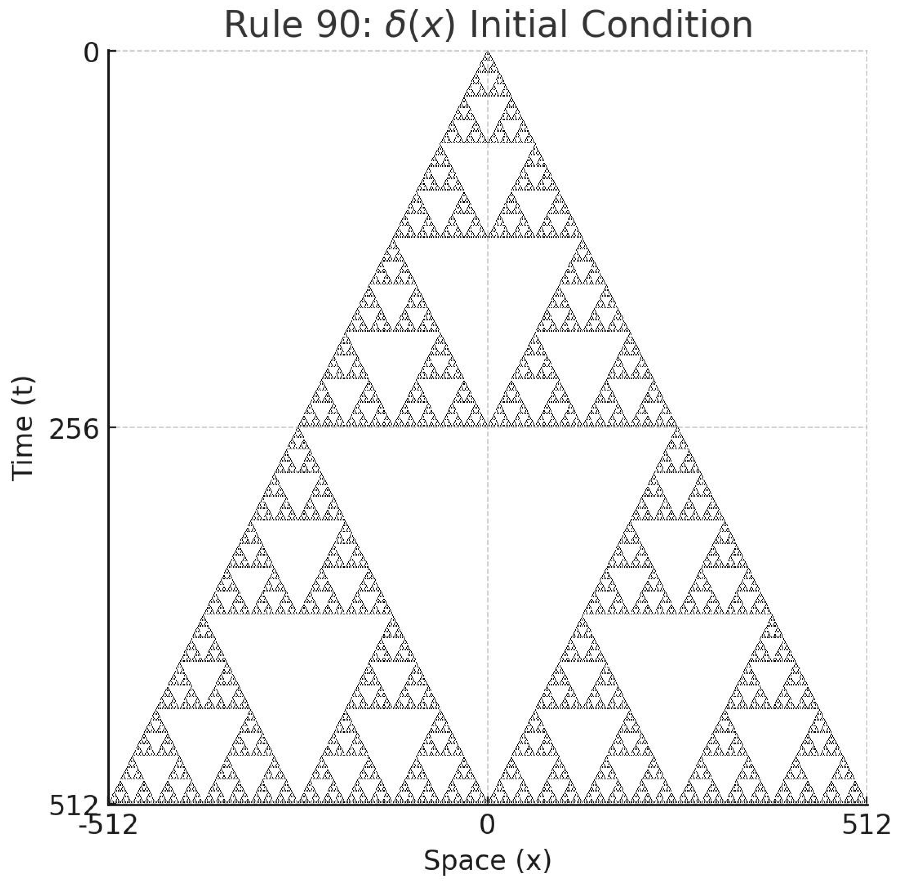
It clearly forms a Sierpiński triangle. Note that each cell’s state depends only on its left and right neighbours. Thus, this fractal is not globally planned, but emerges from local interactions.

Example 2

This is the spatiotemporal plot of Rule 90 with the initial condition $u(0,x)=\delta \left(x\right)$ and boundary conditions $u(t,-100)=u(t,100)=0$.

Figure 3. Spatiotemporal plot of Rule 90 with $u(0,x)=\delta \left(x\right)$ and boundary conditions $u(t,-100)=u(t,100)=0$.

Figure 3. Spatiotemporal plot of Rule 90 with $u(0,x)=\delta \left(x\right)$ and boundary conditions $u(t,-100)=u(t,100)=0$.

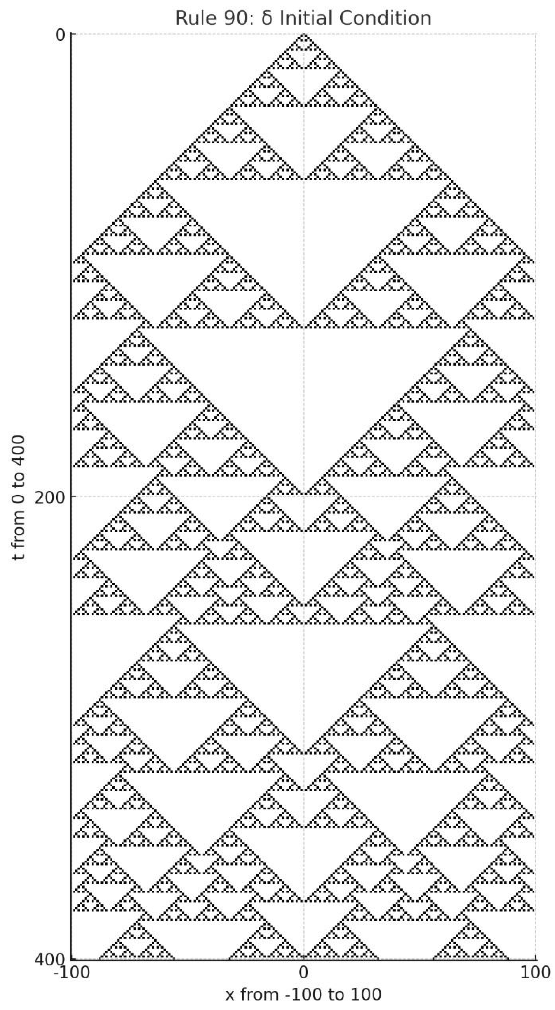
Initially, we observe a perfect Sierpiński triangle. However, once the pattern reaches the boundary, it breaks down into spatiotemporal chaos and becomes unpredictable.

Example 3

This is the spatiotemporal plot of Rule 90 with random initial condition and boundary conditions $u(t,-200)=u(t,200)=0$.

Figure 4. Spatiotemporal plot of Rule 90 with random initial condition and boundary conditions.

Figure 4. Spatiotemporal plot of Rule 90 with random initial condition and boundary conditions.

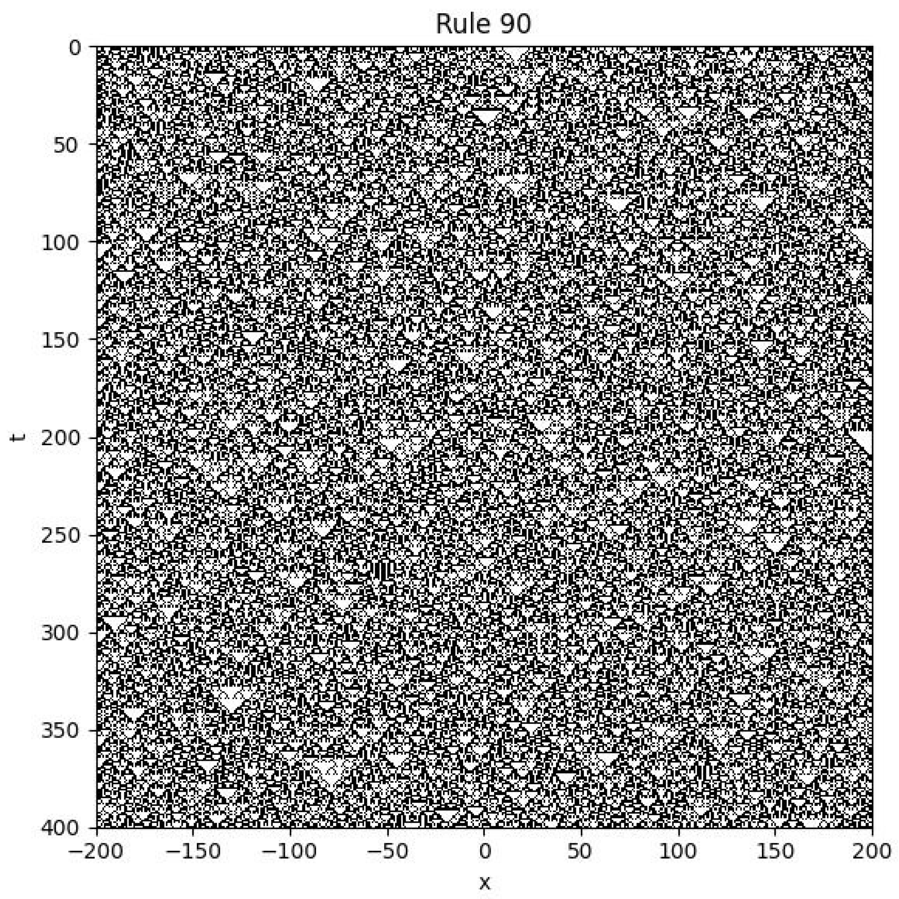
As shown, the system exhibits spatiotemporal chaos.

4.4. Rule 30

The evolution equation for Rule 30, derived using Boolean algebra, is given by:

$$E_{t}u={mod}_2\left(E_x^{-1}u+E_{x}u+u+u·E_{x}u\right),$$

where $E_t$ is the time shift operator, $E_x$ is the spatial right shift operator.

Example

We consider the following simulation setup:

• Initial condition: $u(0,x)$ is chosen randomly with values in $\{0,1\}$.
• Boundary condition: $u(t,-200)=u(t,200)=0$ for all t.

The figure below shows the spatiotemporal evolution of the system under Rule 30:

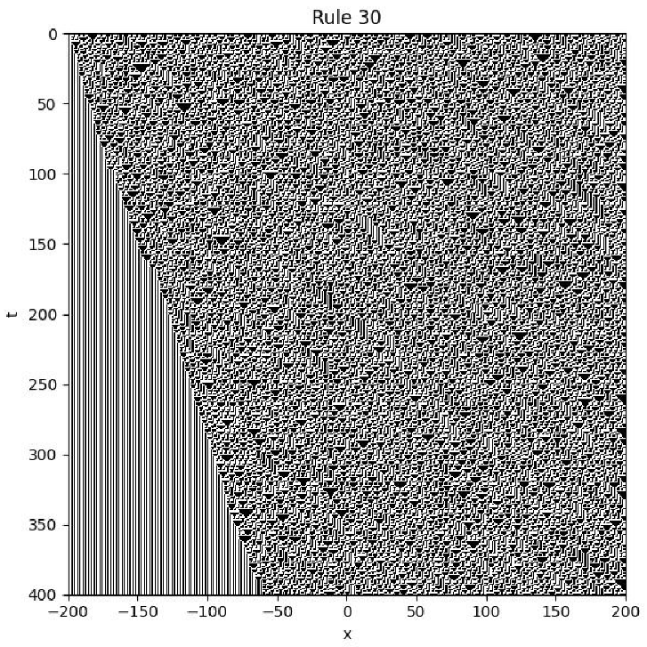
It is evident that the system exhibits spatiotemporal chaos, characterized by aperiodic and unpredictable patterns across both space and time.

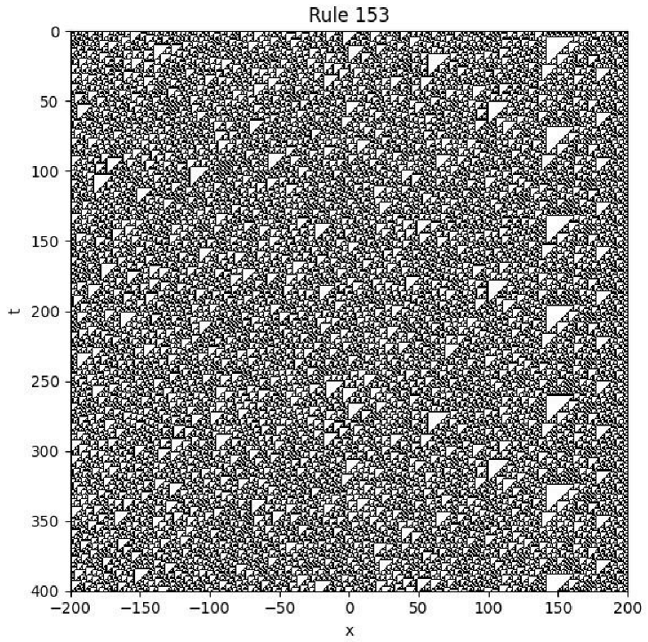
4.5. The Rule 153

We define the evolution equation as follows:

$$E_{t}u={mod}_2\left(⌊{\displaystyle \frac{1-E_x^{-1}u}{1+E_{x}u}}+E_{x}u·E_x^{-1}u+\left|3E_x^{-1}u-4E_{x}u\right|+u⌋\right)$$

Example

• Initial condition: $u(0,x)$ is assigned a random binary value (0 or 1) at each spatial point.
• Boundary condition: $u(t,-200)=u(t,200)=0$ for all t.
• Colour scheme: 0 is shown as white, and 1 is shown as black.

The following image illustrates the space-time evolution from $t=0$ to $t=400$, and $x\in [-200,200]$, with a random initial condition:

This system exhibits spatiotemporal chaos.

4.6. Rule 45

The Boolean update rule for Rule 45 can be written as the following equation:

$$E_{t}u={\mathrm{mod}}_2\left(1+u+E_x^{-1}u+u·E_{x}u\right)$$

Example

Initial condition: $u(0,x)$ is random.

Boundary conditions: $u(t,-200)=u(t,200)=0$.

Figure 5. Spatiotemporal plot of Rule 45 with random initial condition and fixed boundary conditions.

Figure 5. Spatiotemporal plot of Rule 45 with random initial condition and fixed boundary conditions.

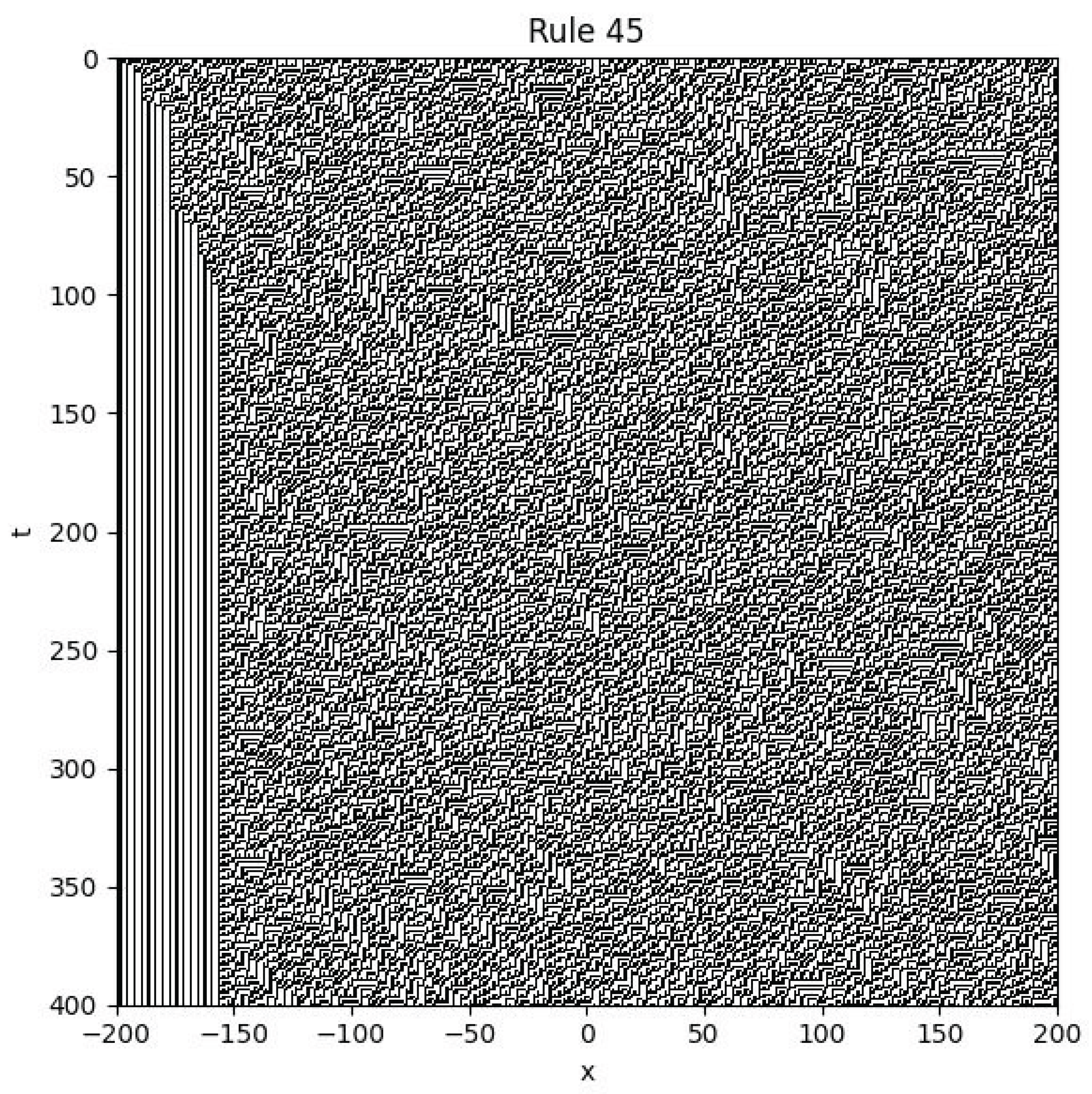
As shown in the figure, this system also exhibits spatiotemporal chaos. The resulting pattern features strange, curled, filament-like structures.

4.7. Rule 105

The Boolean update rule for Rule 105 can be written using logical operations as follows:

$$E_{t}u={\mathrm{mod}}_2\left(E_x^{-1}u·u·\delta \left(E_{x}u\right)+E_x^{-1}u·\delta \left(u\right)·E_{x}u+\delta \left(E_x^{-1}u\right)·u·E_{x}u+\delta \left(E_x^{-1}u\right)·\delta \left(u\right)·\delta \left(E_{x}u\right)\right)$$

Here, $\delta \left(x\right)$ denotes the Boolean NOT operation.

Example

Initial condition: $u(0,x)$ is random.

Boundary conditions: $u(t,-200)=u(t,200)=0$.

Figure 6. Spatiotemporal plot of Rule 105 with random initial condition and fixed boundaries.

Figure 6. Spatiotemporal plot of Rule 105 with random initial condition and fixed boundaries.

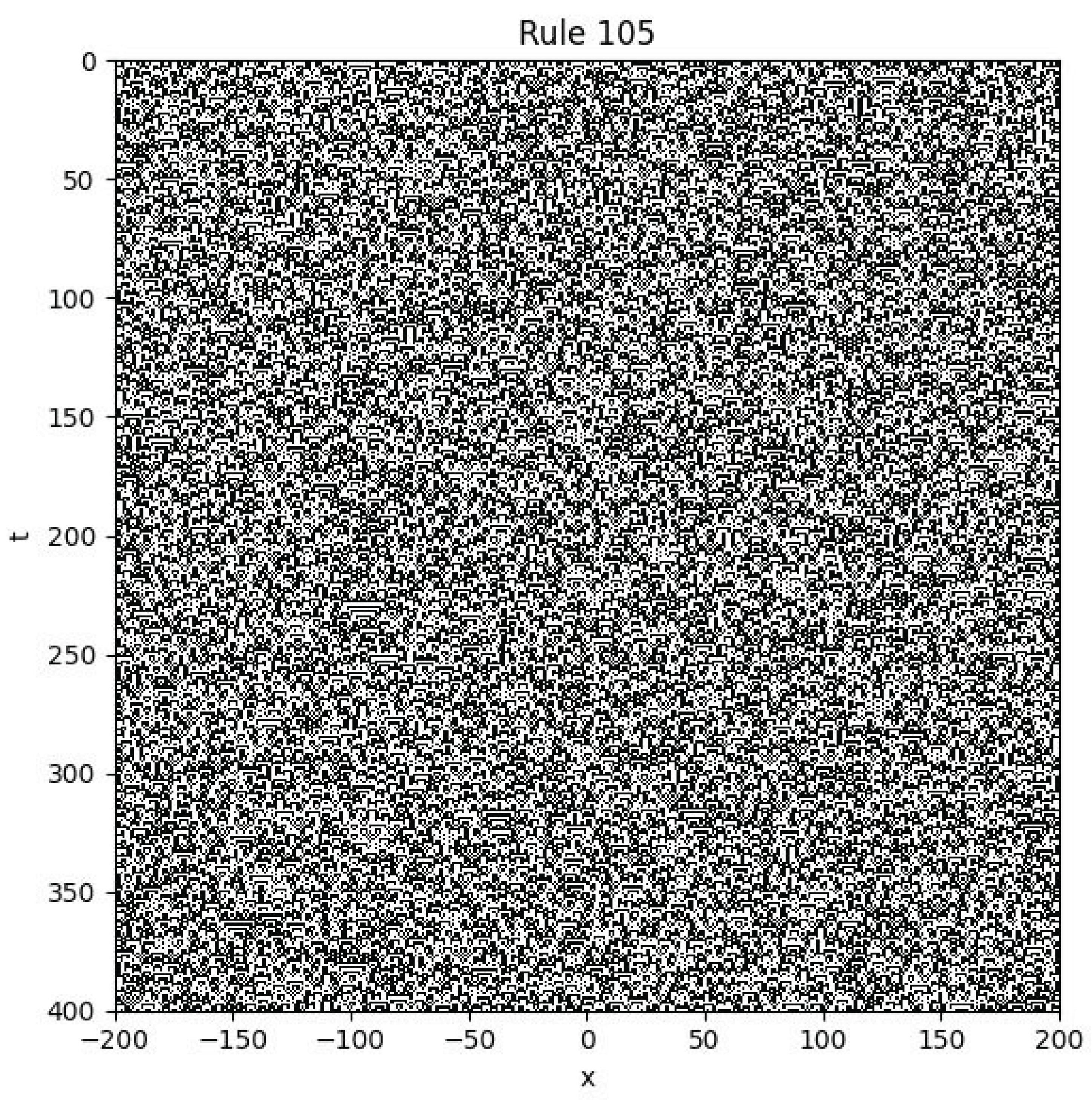
As shown in the figure, this system also exhibits spatiotemporal chaos. The resulting pattern consists of intricate structures resembling scales or rippling textures.

4.8. Rule 169

The Boolean update rule for Rule 169 can be expressed as:

$$E_{t}u={\mathrm{mod}}_2\left(E_x^{-1}u·u+E_x^{-1}u+u+E_{x}u+1\right)$$

Example

Initial condition: $u(0,x)$ is random.

Boundary conditions: $u(t,-200)=u(t,200)=0$.

Figure 7. Spatiotemporal plot of Rule 169 with random initial condition and fixed boundaries.

Figure 7. Spatiotemporal plot of Rule 169 with random initial condition and fixed boundaries.

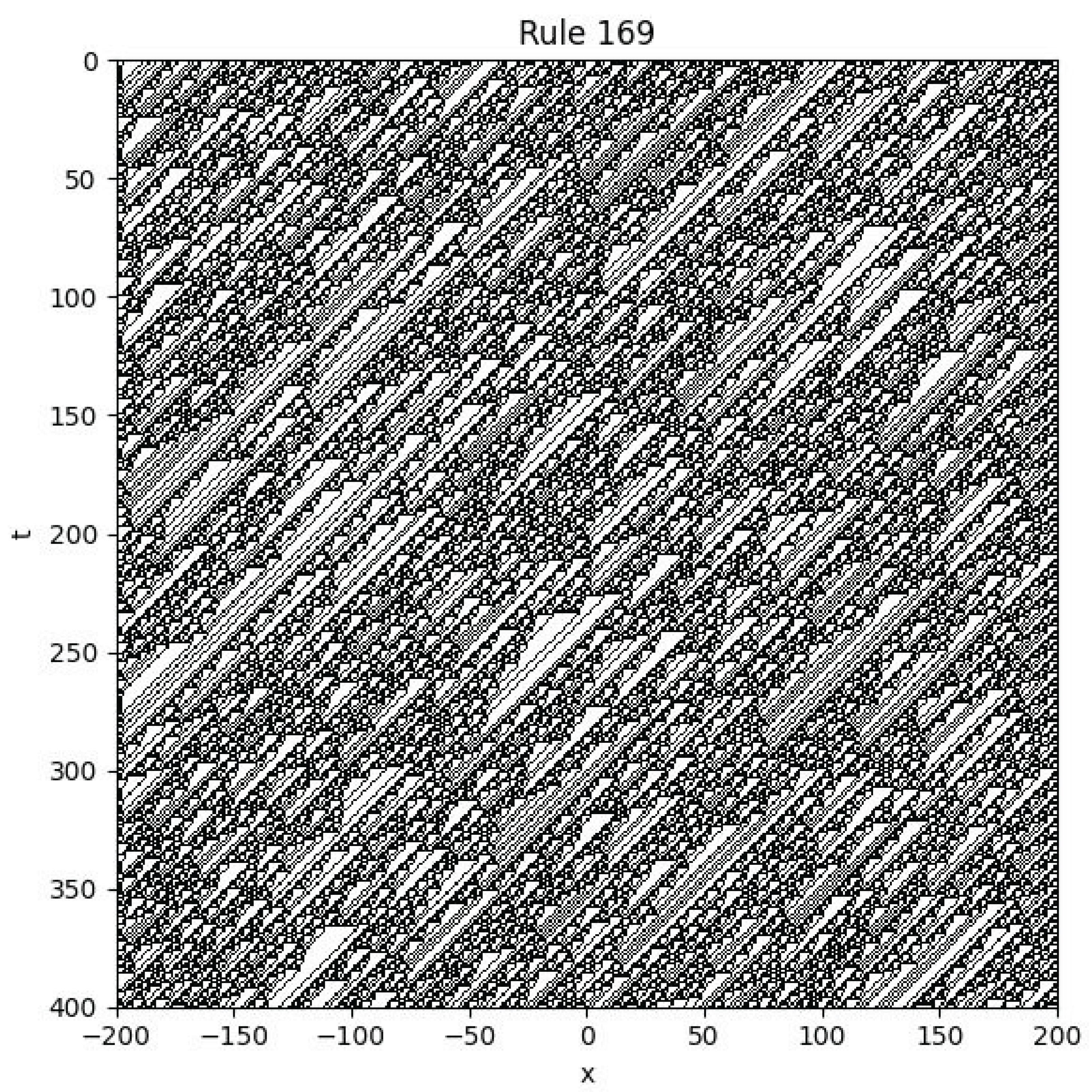
As shown in the figure, the system exhibits spatiotemporal chaos. The resulting patterns resemble diagonal stalactites, indicating complex local interactions and emergent behaviour.

4.9. Rule 210

The Boolean update rule for Rule 210 is given by:

$$E_{t}u={\mathrm{mod}}_2\left(E_x^{-1}u·u·E_{x}u+E_x^{-1}u·u·\delta \left(E_{x}u\right)+E_x^{-1}u·\delta \left(u\right)·\delta \left(E_{x}u\right)+\delta \left(E_x^{-1}u\right)·\delta \left(u\right)·E_{x}u\right)$$

Example

Initial condition: $u(0,x)$ is random.

Boundary conditions: $u(t,-200)=u(t,200)=0$.

Figure 8. Spatiotemporal plot of Rule 210 with random initial condition and fixed boundaries.

Figure 8. Spatiotemporal plot of Rule 210 with random initial condition and fixed boundaries.

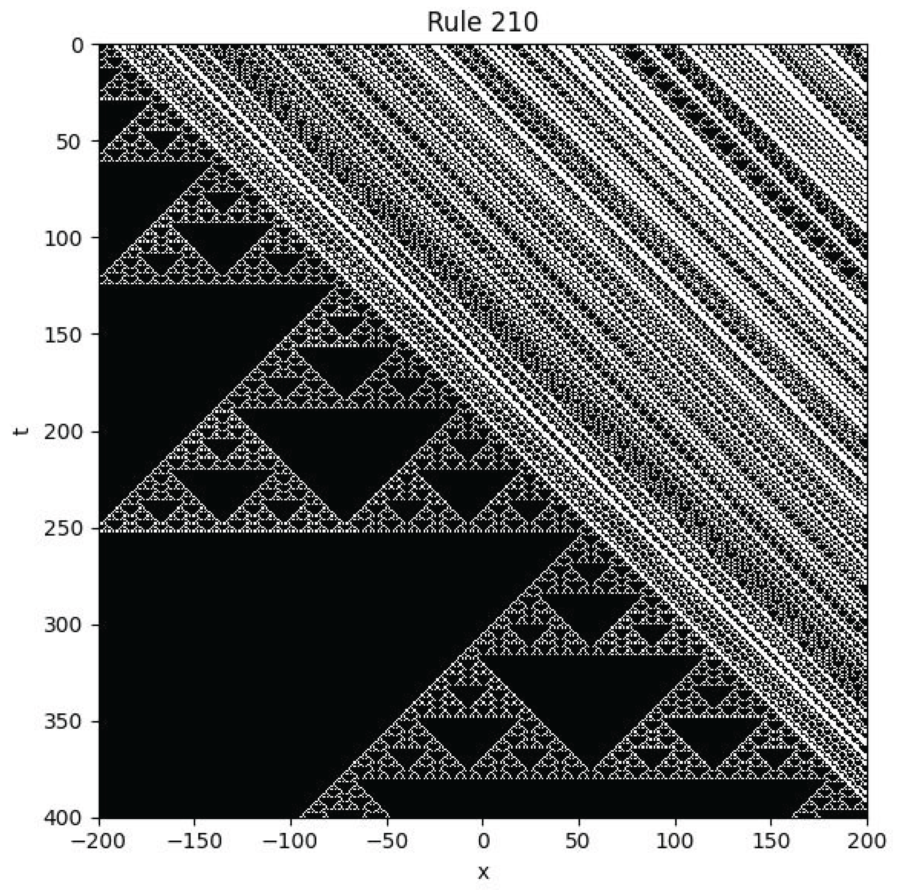
As shown in the figure, the system exhibits a highly unusual structure: one region resembles a Sierpiński triangle, while the other shows diagonally arranged motifs. This dual pattern reflects complex local interactions and potentially bifurcating spatial dynamics.

4.10. Rule 137

We define the evolution equation as follows:

$$E_{t}u={mod}_2\left(\left|⌊\left(E_x^{-1}u-{\pi }^u\right)\left(\pi +u+E_{x}u\right)⌋\right|+⌊\left|{\displaystyle \frac{1-u}{1+u}}\right|⌋+\left|3E_x^{-1}u-4u\right|\right)$$

each state value satisfies

$$u(t,x)\in \{0,1\}.$$

This rule is an example of a nonlinear partial difference equation, operating over a binary state space.

Interestingly, the system exhibits a mixture of order and apparent randomness. Some regions evolve into highly regular patterns, while others appear chaotic and unpredictable. This suggests that the system may operate near the edge of chaos, a regime known for its potential computational richness and complexity.

Although we do not currently possess a closed-form analytic solution to this equation, the intricate structure of its evolving patterns can still be studied using tools such as combinatorics, discrete functional analysis, and spatiotemporal statistics.

Example

Initial condition: $u(0,x)$ is random.

Boundary conditions: $u(t,-200)=u(t,200)=0$.

Figure 9. Spatiotemporal plot of Rule 137 with random initial condition and fixed boundaries.

Figure 9. Spatiotemporal plot of Rule 137 with random initial condition and fixed boundaries.

The pattern generated by Rule 137 closely resembles that of Rule 110. It exhibits complex behaviour with both periodic islands and chaotic seas. There are large regions of crystalline structure, along with distinct triangular motifs, indicating rich dynamics and spatial self-organization.

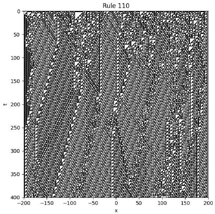
4.11. Rule 110

Using Boolean algebra, we derive the evolution equation for Rule 110 as follows:

$$E_{t}u={mod}_2\left(u+E_{x}u+u·E_{x}u+u·E_{x}u·E_x^{-1}u\right),$$

where $E_t$ denotes the time shift operator, $E_x$ is the spatial right-shift operator, and ${mod}_2$ denotes addition modulo 2.

Example

We consider the following setup:

• Initial condition: $u(0,x)$ is chosen randomly with values in $\{0,1\}$.
• Boundary condition: $u(t,-200)=u(t,200)=0$ for all t.

The figure below illustrates the space-time evolution of the system under Rule 110:

5. Other 1D Nonlinear Partial Difference Equations

5.1. Introduction

Beyond classical two-state cellular automata such as Rule 90 or Rule 137, we have discovered that a wide variety of other one dimensional nonlinear partial difference equations (P$\Delta$E) can be constructed. These equations may involve arithmetic operations, logical operations, or floor and absolute value functions. They do not necessarily follow the strict rule-based framework of cellular automata, yet they remain fully deterministic and discrete in both space and time.

Such equations often exhibit rich and unexpected dynamical behaviour. Some generate spatially localized chaos, while others display periodic or quasiperiodic structures. This diversity suggests that one-dimensional nonlinear P$\Delta$E form a broader and more general class of systems than traditionally studied automata.

In the following subsections, we will explore several such examples and discuss their qualitative features.

5.2. Sierpinski Fan Equation

Consider the following nonlinear partial difference equation:

$$E_{t}u={mod}_3\left(E_x^{-1}u+u+E_{x}u\right)$$

with initial condition:

$$u(0,x)=\delta \left(x\right),\mathrm{and}\mathrm{no}\mathrm{boundary}\mathrm{condition}.$$

$u=u(t,x)\in \{0,1,2\}$ Here, the delta function $\delta \left(x\right)$ is defined as:

$$\delta \left(x\right)=\left\{\begin{array}{cc}1,\hfill & x=0\hfill \\ 0,\hfill & x\ne 0\hfill \end{array}\right.$$

This system produces a fascinating fractal structure resembling a "fan" or "tree", hence we refer to it as the Sierpinski Fan Equation.

Although we currently do not have an analytic solution to this equation, the emergent pattern clearly exhibits self-similarity and modular periodicity, which are typical features of modular arithmetic-driven cellular automata. This suggests a rich underlying structure that deserves further investigation.

Figure 10. Spatiotemporal evolution of the Sierpinski Fan Equation

Figure 10. Spatiotemporal evolution of the Sierpinski Fan Equation

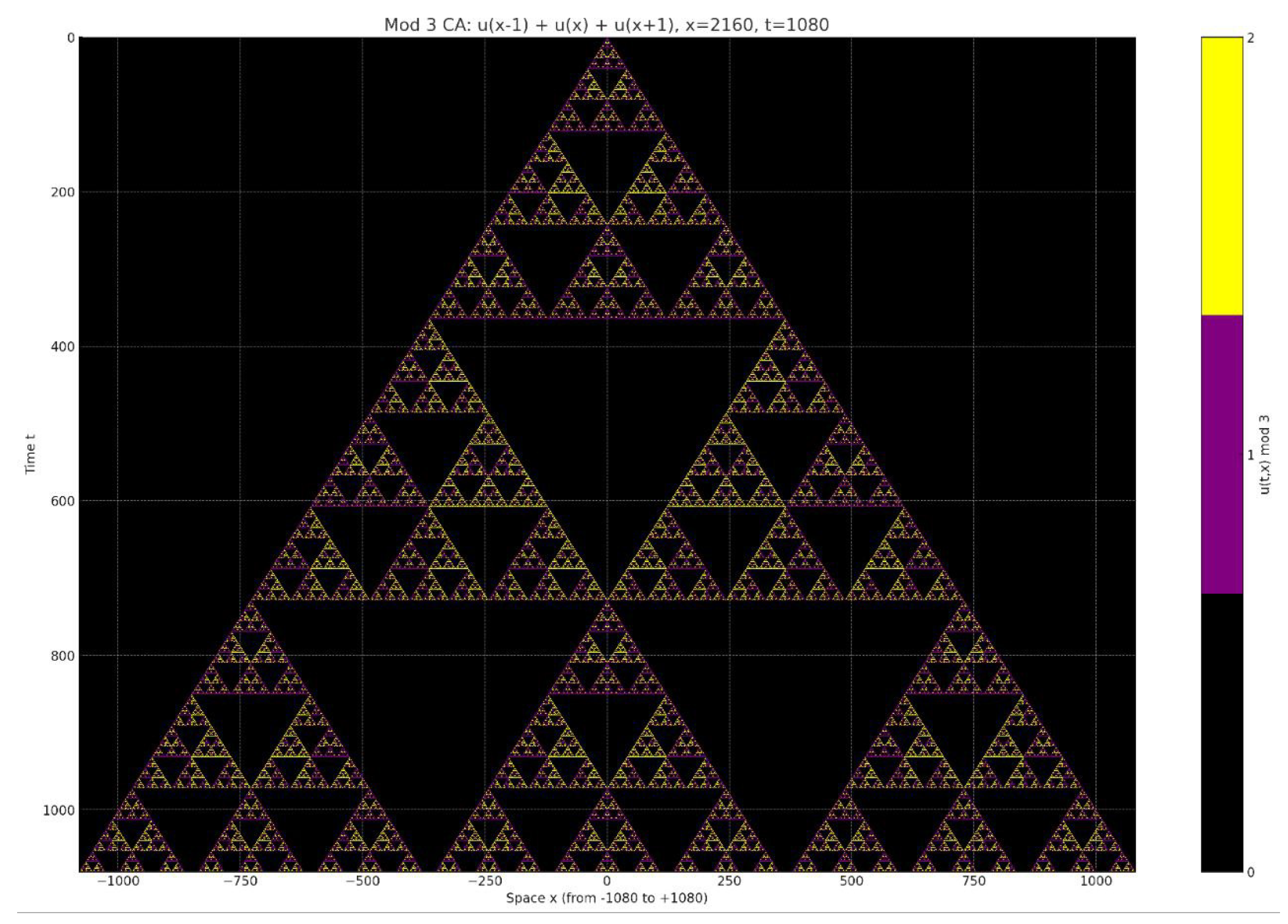
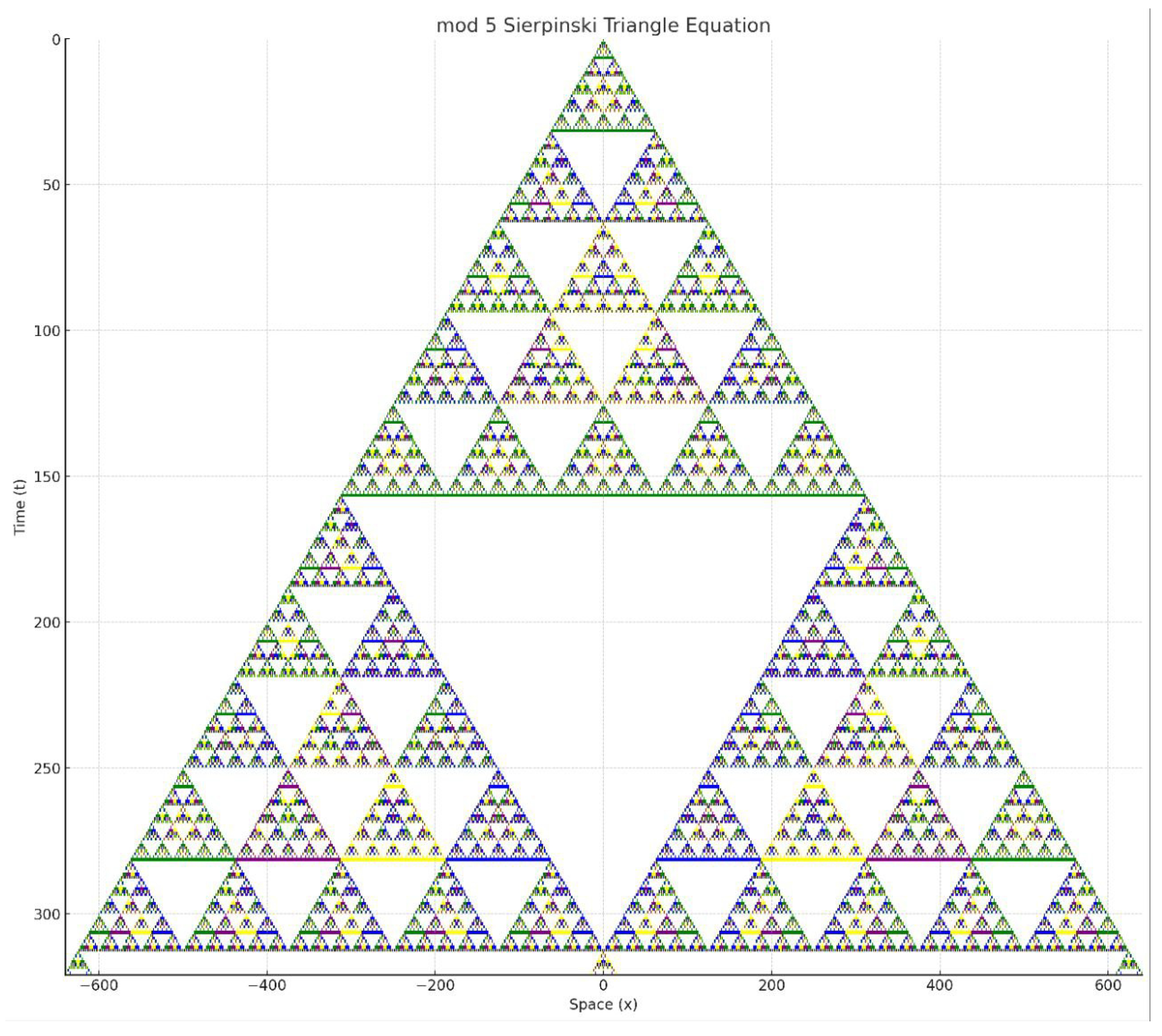
5.3. Mod 5 Sierpiński Equation

We define a new nonlinear partial difference equation as follows:

$$E_{t}u={mod}_5\left(E_x^{-2}u+E_x^{-1}u+u+E_x^{1}u+E_x^{2}u\right)$$

with the initial condition:

$$u(0,x)=\delta \left(x\right)$$

where:

• $\delta \left(x\right)$ is the discrete delta function defined by $\delta \left(x\right)=1$ if $x=0$, and 0 otherwise;
• $u=u(t,x)\in \{0,1,2,3,4\}$ for all $t,x$;
• The system is updated on a discrete 1D lattice with no boundary condition.

This equation can be seen as a generalization of the Rule 90 or Sierpiński triangle in modulo 2. The modulo 5 version creates a far richer fractal structure.

From the spatiotemporal plot, we observe that instead of the classic single upside-down triangle in each upright triangle (as in the binary Sierpiński triangle), this pattern exhibits ten upside-down triangles within each upright triangle. This suggests a more intricate self-similar structure with higher-order modular symmetry.

We call this the Mod 5 Sierpiński Equation.

5.4. Mod 4 Sierpinski Fractal Equation

We consider the following nonlinear partial difference equation:

$$E_{t}u={mod}_4\left(E_x^{-1}u+u+E_{x}u+\delta \left(x\right)\right)$$

with initial condition:

$$u(0,x)=\delta \left(x\right)$$

and no boundary condition.

Figure 11. Spatiotemporal evolution of the Mod 5 Sierpiński Equation

Figure 11. Spatiotemporal evolution of the Mod 5 Sierpiński Equation

$u=u(t,x)\in \{0,1,2,3\}$

Here, $\delta \left(x\right)$ is the discrete delta function defined by:

$$\delta \left(x\right)=\left\{\begin{array}{cc}1,\hfill & \mathit{if}x=0\hfill \\ 0,\hfill & \mathrm{otherwise}\hfill \end{array}\right.$$

The values of $u(t,x)$ are restricted to $\{0,1,2,3\}$, and we visualize them using the following colour scheme:

Value	Colour
0	White
1	Green
2	Purple
3	Yellow

The spatiotemporal plot of this equation is shown below:

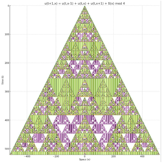
We observe that this system generates a strikingly complicated fractal structure, reminiscent of a Sierpinski triangle, but with richer periodic colour layers. Despite its simplicity, the system exhibits highly nontrivial dynamics that may reflect deep combinatorial or algebraic patterns.

6. Coupled Map Lattice

6.1. 1D Coupled Map Lattice

The one-dimensional Coupled Map Lattice (CML), originally proposed by Kaneko [9], is a prototypical model for spatiotemporal chaos. It is defined by the following recurrence relation:

$$u_s^{t+1}=(1-\epsilon )f\left(u_s^t\right)+{\displaystyle \frac{\epsilon }{2}}\left(f\left(u_{s+1}^t\right)+f\left(u_{s-1}^t\right)\right),$$

where $u_s^t\in \mathbb{R}$, $f:\mathbb{R}\to \mathbb{R}$ is a nonlinear local map (e.g., logistic map), and $\epsilon \in [0,1]$ is the coupling strength.

We reformulate this equation using shift operators to obtain a compact operator-based representation:

$$E_{t}u=(1-\epsilon )f\left(u\right)+{\displaystyle \frac{\epsilon }{2}}\left(f\left(E_{x}u\right)+f\left(E_x^{-1}u\right)\right),$$

where

$$u=u(t,x),u:{\mathbb{Z}}^2\to \mathbb{R}.$$

This equation is usually nonlinear autonomous Partial Difference Equation that captures spatiotemporal dynamics and is frequently used to model chaotic behaviour on discrete lattices.

6.2. 2D Coupled Map Lattice

The two-dimensional Coupled Map Lattice (2D CML) extends the 1D case to a square lattice, where each site interacts with its four nearest neighbours. The classical form is given by:

$$u_{i,j}^{t+1}=(1-\epsilon )f\left(u_{i,j}^t\right)+{\displaystyle \frac{\epsilon }{4}}\left[f\left(u_{i+1,j}^t\right)+f\left(u_{i-1,j}^t\right)+f\left(u_{i,j+1}^t\right)+f\left(u_{i,j-1}^t\right)\right],$$

where $u_{i,j}^t\in \mathbb{R}$, $f:\mathbb{R}\to \mathbb{R}$, and $\epsilon \in [0,1]$ as before.

Using shift operators, the system can be rewritten in a compact operator-based form:

$$E_{t}u=(1-\epsilon )f\left(u\right)+{\displaystyle \frac{\epsilon }{4}}\left[f\left(E_{x}u\right)+f\left(E_x^{-1}u\right)+f\left(E_{y}u\right)+f\left(E_y^{-1}u\right)\right],$$

where

$$u=u(t,x,y),u:{\mathbb{Z}}^3\to \mathbb{R}.$$

This operator representation highlights the spatial symmetry and facilitates generalization to higher dimensions, anisotropic coupling, or graph-based topologies.

6.3. Explanation

A coupled map lattice (CML) is a discrete-time, discrete-space dynamical system in which each lattice site evolves according to a prescribed local map and interacts with other sites via a coupling rule. The local map encodes the nonlinear dynamics at each site, while the coupling represents spatial interactions such as diffusion, transport, or synchronization.

CMLs are capable of producing spatiotemporal chaos, where complex, irregular patterns emerge and evolve across both space and time. They occupy an intermediate position between continuous partial differential equations and fully discrete cellular automata: like PDE, they describe the evolution of a field; like CA, they are inherently discrete in space and time.

In the context of this work, CMLs can be regarded as a particular subclass of partial difference equations in which the update operator contains a nonlinear local component together with a discrete coupling term. This perspective allows the mathematical machinery of discrete functional analysis to be applied directly to the study of CML dynamics.

7. The Conway’s Game of Life

7.1. Conway’s Equation

We express Conway’s Game of Life [4] as a nonlinear autonomous partial difference equation:

$$E_{t}u=\delta (u-1)\left[\delta (S_{M}u-2)+\delta (S_{M}u-3)\right]+\delta \left(u\right)\delta (S_{M}u-3)$$

where the neighbourhood sum is defined as:

$$S_{M}u:=\sum _{(i,j)\in M}{E}_x^i{E}_y^{j}u$$

with the following definitions:

• $u=u(t,x,y)\in \{0,1\}$ is the binary state of the cell at time t and position $(x,y)$, where 1 denotes "alive" and 0 denotes "dead".
• $E_t,E_x,E_y$ are the forward shift operators in time and spatial directions, respectively.
• M is the Moore neighbourhood excluding the center, i.e., the set of 8 nearest neighbours:

  $$M=\left\{\right(-1,-1),(-1,0),(-1,1),(0,-1),(0,1),(1,-1),(1,0),(1,1\left)\right\}$$
• $\delta \left(x\right)$ is the Kronecker delta function, defined as:

  $$\delta \left(x\right)=\left\{\begin{array}{cc}1\hfill & \mathit{if}x=0\hfill \\ 0\hfill & \mathrm{otherwise}\hfill \end{array}\right.$$

This formulation represents a nonlinear autonomous partial difference equation, where the next state of each cell depends only on its current state and the sum of its neighbours in the Moore neighbourhood.

7.2. Interpretation

We observe that: - Still lifes are the steady-state solution. - Gliders behave like solitons, stable moving structures. - Oscillators resemble standing waves, periodically repeating in place. - Each of these localized configurations can be seen as a local attractor unit. - Multiple local attractors can couple together, forming a large-scale network we call the Attractor Coupling Network (ACN).

This structure is: - A dynamic fractal network, in the sense that it exhibits recursive nesting: a network within a network, evolving over time. - Capable of universal computation: Conway’s Game of Life is known to be Turing complete.

This suggests a deep connection between simple discrete dynamics and the emergence of complex, structured, and computationally powerful behaviour.

8. Abelian Sandpile Model

8.1. Abelian Sandpile Equation

The evolution of the Abelian Sandpile Model [3] is given by the following equation:

$${\displaystyle E_{t}u=u-4\theta (u-4)+\sum _{(i,j)\in V}\theta \left(E_x^i{E}_y^{j}u-4\right)+G(t,x,y)}$$

where:

• $u(t,x,y)\in \{0,1,2,3\}$
• $\theta \left(x\right)$ is the Heaviside step function:

  $$\theta \left(x\right)=\left\{\begin{array}{cc}1,\hfill & \mathit{if}x\ge 0\hfill \\ 0,\hfill & \mathrm{otherwise}\hfill \end{array}\right.$$
• V is the von Neumann neighbourhood:

  $$V=\left\{\right(1,0),(-1,0),(0,1),(0,-1\left)\right\}$$
• $G(t,x,y)$ is the external forcing term (i.e., the addition of sand grains)

8.2. Remarks

This is a Non-Autonomous Partial Difference Equation.

This is a classical model of Self-Organized Criticality (SOC). It exhibits:

• Emergent fractal patterns
• Scale-invariant avalanches
• Critical behaviour without parameter fine-tuning

For a deeper understanding of self-organized criticality in sandpile models, see [3].

8.3. The Sandpile Fractal

If the forcing term is given by

$$G(t,x,y)=\delta \left(x\right)\delta \left(y\right),$$

with initial condition

$$u(0,x,y)=0,$$

and no boundary condition imposed, then the solution exhibits a fractal structure resembling the classical sandpile model. The resulting pattern looks as follows:

Figure 2. Fractal structure generated by dropping 30 million grains at a single site on the infinite square lattice and applying the rules of the Abelian sandpile model. Image by colt_browning, from Wikipedia, licensed under CC BY 4.0. Code: github.com/colt-browning/sandpile.

Figure 2. Fractal structure generated by dropping 30 million grains at a single site on the infinite square lattice and applying the rules of the Abelian sandpile model. Image by colt_browning, from Wikipedia, licensed under CC BY 4.0. Code: github.com/colt-browning/sandpile.

8.4. Extended Sandpile Model

We present an extended version of the Abelian Sandpile Model in which each site topples only when it contains at least 8 grains of sand. The neighbourhood used here is the Moore neighbourhood, which includes the 8 surrounding cells (horizontal, vertical, and diagonal neighbours).

The evolution equation of the system is given by:

$$E_{t}u=u-8\theta (u-8)+\sum _{(i,j)\in M}\theta (E_x^i{E}_y^{j}u-8)+G(t,x,y)$$

where:

• $u=u(t,x,y)$ represents the number of sand grains at position $(x,y)$ and time t,
• $\theta$ is the Heaviside step function,
• M denotes the Moore neighbourhood:
  $M=\left\{\right(-1,-1),(-1,0),(-1,1),(0,-1),(0,1),(1,-1),(1,0),(1,1\left)\right\}$,
• $G(t,x,y)$ is an external sand input term.

Example

• Initial Condition: $u(0,x,y)=0$
• Boundary Condition: None (infinite or sufficiently large grid with no boundary constraints)
• Forcing Term: $G(t,x,y)=\delta \left(x\right)\delta \left(y\right)$ (unit sand grain dropped at the center)

The figure below shows the configuration $u(500000,x,y)$ after 500,000 iterations:

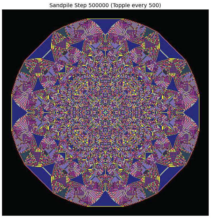
We observe that the resulting pattern resembles the classical sandpile model, but exhibits greater complexity due to the use of the Moore neighbourhood and the 8-grain threshold. The colours are more diverse, and the structure appears more intricate and vibrant.

8.5. Explanation for the Self-Organized Criticality

Consider the comparison between Rule 90 and the Sandpile model. Rule 90 is defined by the update rule:

$$E_{t}u={\mathrm{mod}}_2\left(E_x^{-1}u+E_{x}u\right)$$

Both Rule 90 and the Sandpile model are based on local interactions and exhibit nonlinear dynamics. However, they display drastically different macroscopic behaviours: Rule 90 leads to global chaos, while the Sandpile model exhibits self-organized criticality.

In Rule 90, any small perturbation is exponentially amplified due to the absence of thresholds, every update directly sums the neighbouring values modulo 2, regardless of the current state. As a result, the system exhibits global sensitivity to initial conditions, a hallmark of chaos.

In contrast, the Sandpile model incorporates a threshold-based collapse mechanism. Before any site reaches the threshold (typically 4 in 2D), the system behaves linearly: each grain of sand simply increases the local state by 1. Once the threshold is reached, a toppling event occurs, distributing sand to neighbours and potentially triggering further topplings. This collapse phase introduces nonlinearity and chaotic propagation, but only in localized regions that have reached the critical state.

Therefore, the Sandpile model alternates between two distinct regimes:

• Linear growth phase: Sites far below the threshold evolve smoothly and predictably.
• Chaotic collapse phase: Sites at the threshold trigger avalanches with unpredictable, nonlinear dynamics.

Because the initial configuration is typically random, some sites are near-zero (linear regime), while others are near the threshold (nonlinear regime). This coexistence of order and chaos in space and time allows the Sandpile model to maintain a dynamically balanced state without the need for fine-tuning of parameters.

This explains why the Sandpile model self-organizes into a critical state: the rules themselves inherently support a mixture of linear and chaotic zones, allowing the system to spontaneously hover at the edge of chaos. Unlike systems that require tuning to a critical point, the Sandpile model exhibits critical behaviour as an emergent property of its local update rules.

8.6. Explanation for the Power Law Distribution

The avalanche size distribution in the Sandpile model follows a power law, typically of the form:

$$P\left(s\right)\propto s^{-\tau }$$

where $P\left(s\right)$ is the probability of an avalanche of size s, and $\tau$ is a constant exponent. This behaviour arises from the interplay between local dynamics, chaotic propagation, and external driving. We explain it in three parts:

• Why are small avalanches more common than large ones?
  Because the dynamics are based on local interactions, triggering a large avalanche requires a long chain of causally connected sites to be near the threshold, which is statistically less likely. In contrast, small avalanches require only a short chain and are thus much more probable.
• Why do large avalanches still occur frequently (not exponentially rare)?
  The collapse dynamics are chaotic: once a critical site topples, small perturbations can lead to unpredictable and explosive cascades, this is the butterfly effect. Therefore, even though rare, large avalanches are possible due to the system’s inherent sensitivity at the critical state.
• Why is there no characteristic scale in avalanche size?
  The update rules impose no intrinsic limit on the spatial extent of an avalanche. The avalanche size depends entirely on the current configuration of the system. If a small localized region is near-critical, only a small avalanche occurs. But if a large domain is close to the threshold, a large avalanche may follow. Furthermore, the external driving is random and slow, allowing the system to evolve into configurations where large avalanches are statistically allowed. Thus, the system exhibits scale-invariant behaviour.

9. OFC Earthquake Model

9.1. OFC Earthquake Equation

The Olami-Feder-Christensen (OFC) Model [10] is a discrete-time cellular automaton designed to simulate earthquake dynamics using a self-organized criticality (SOC) framework. The model evolves according to the following partial difference equation:

$$E_{t}u=u-\theta (u-1)+\alpha \sum _{(i,j)\in V}\theta (E_x^i{E}_y^{j}u-1)+G(t,x,y)$$

where:

• $u=u(t,x,y)\in \left[0,1\right]$ represents the local shear stress (or load) at site $(x,y)$ at time t, $u:{\mathbb{Z}}^3\to \mathbb{R}$.
• $E_{t}u=u(t+1,x,y)$ denotes the stress at the next time step.
• $\theta \left(x\right)$ is the Heaviside function, defined as:

  $$\theta \left(x\right)=\left\{\begin{array}{cc}1,\hfill & \mathrm{if}x\ge 0\hfill \\ 0,\hfill & \mathrm{otherwise}\hfill \end{array}\right.$$
• $\alpha {\sum }_{(i,j)\in V}\theta (E_x^i{E}_y^{j}u-1)$ represents the redistributed stress received from neighbouring sites $(i,j)\in V$ that have exceeded the failure threshold. $\alpha$ is a constant.
• $G(t,x,y)$ is an external driving term, typically very small, which represents slow tectonic loading. In most implementations, $G(t,x,y)=\epsilon$ at a randomly selected site and zero elsewhere, modeling slow, local buildup of stress.

The stress u is usually constrained within the interval $[0,1)$, with the threshold for failure set at $u=1$. When $u\ge 1$, the site fails, redistributes stress to its neighbours, and resets or reduces its own stress, initiating potential cascades (earthquake avalanches) through the system.

This model is analogous to the sandpile model but includes continuous-valued stress and dissipation, making it more suitable for simulating earthquake-like events in tectonic systems.

9.2. Observations and Phenomena

The Olami–Feder–Christensen (OFC) earthquake model exhibits dynamics similar to the sandpile model. It demonstrates a power-law distribution in event sizes, where small avalanches occur frequently, while large avalanches are rare. This behaviour is a hallmark of self-organized criticality (SOC), indicating that the system naturally evolves toward a critical state without fine-tuning of parameters.

10. Forest Fire Model

10.1. Forest Fire Equation

We define the forest fire dynamics on a discrete lattice as a Partial Difference Equation with mod-3 state cycling [11]:

$$E_{t}u={mod}_3\left(2\delta (u-1)\theta (S-1)+G(t,x,y)\right)$$

$$S=\sum _{(i,j)\in M}\delta \left(E_x^i{E}_y^{j}u-2\right)$$

10.2. Definitions

• $u=u(t,x,y)\in \{0,1,2\}$ is the state of the cell at time t and spatial coordinates $(x,y)$.

• 0: empty ground (bare land)
-
1: tree
-
2: burning tree
• $E_t$ is the forward time shift operator: $E_{t}u:=u(t+1,x,y)$
• $E_x^i{E}_y^{j}u:=u(t,x+i,y+j)$ are spatial shift operators in the Moore neighbourhood M.
• $\delta \left(n\right)$ is the Kronecker delta function: $\delta \left(n\right)=1$ if $n=0$, else 0.
• $\theta \left(x\right)$ is the Heaviside step function: $\theta \left(x\right)=1$ if $x\ge 0$, else 0.
• $G(t,x,y)\in \{0,1\}$ is the non-autonomous external driving force:

  -

  $G=0$: no external change

  -

  $G=1$: apply one-step growth/fire transition (see below)

10.3. Transition Logic (via mod 3)

The entire system evolves via modular arithmetic:

$$\mathrm{New}\mathrm{state}={mod}_3\left(\mathrm{current}\mathrm{state}+\mathrm{external}\mathrm{or}\mathrm{fire}-\mathrm{induced}\mathrm{increment}\right)$$

• $0\stackrel{+1}{\to }1$: tree grows on empty land
• $1\stackrel{+1}{\to }2$: tree catches fire
• $2\stackrel{+1}{\to }0$: burning tree becomes ash (empty)

This simple cyclic structure captures the dynamics of vegetation growth, fire propagation, and destruction.

10.4. Interpretation

A tree at $(x,y)$ will ignite if: - Its current state is 1 (tree), and - There is at least one burning tree in its neighbourhood ($S\ge 1$)

Otherwise, only external driving force $G(t,x,y)$ determines its evolution.

10.5. Observations and Phenomena

We consider the autonomous equation of the Forest Fire Model, and using Moore Neighbourhood. Numerical simulations reveal that the global behaviour of the system is highly sensitive to the initial condition, particularly the forest density.

Assume the initial condition where the entire leftmost column of the grid is set on fire, and all other cells are either trees or empty ground according to a prescribed forest density. We observe the following distinct behaviours:

• Low density (e.g., 10%): The fire fails to propagate. Due to the sparsity of trees, the flame quickly extinguishes after burning only a few connected trees.
• High density (e.g., 80%): The fire spreads rapidly and extensively. Almost the entire forest is consumed in a short period, with the flame front advancing in a nearly uniform and predictable wave.
• Intermediate density (e.g., around 40%): A highly nontrivial behaviour emerges. The fire propagates in an irregular, branching manner, forming a complex fractal-like structure. The fire path becomes winding, unpredictable, and sensitive to small variations in the initial configuration.

This suggests the existence of a critical threshold of forest density that separates the extinguishing, fractal, and total-burning regimes. The system exhibits characteristics of critical phenomena and self-organized complexity at intermediate densities.

11. Kuramoto Firefly Model

11.1. Kuramoto Equation

We define the Kuramoto model as a discrete phase-coupled oscillator network evolving on a 2D grid:

$$E_{t}u={mod}_{2\pi }\left(u+w(x,y)+{\displaystyle \frac{K}{8}}\sum _{(i,j)\in M}sin(E_x^i{E}_y^{j}u-u)\right)$$

• $u=u(t,x,y)\in \left[0,2\pi \right]$ is the phase at grid point $(x,y)$ and time t.
• $w(x,y)$ is a fixed intrinsic frequency assigned randomly to each point.
• K is the coupling constant. In our simulations, we choose $K=1$.
• M is the Moore neighbourhood:

  $$M=\left\{\right(\pm 1,0),(0,\pm 1),(\pm 1,\pm 1\left)\right\}$$

11.2. Principle of Locality

In the original Kuramoto model, oscillators are globally coupled, each unit interacts with every other oscillator in the system.  [12]. While this assumption simplifies mathematical analysis, it is biologically implausible. For example, it is unreasonable to assume that a firefly can perceive and compute the phases of all other fireflies in the environment at each time step.

To address this limitation, we propose the Kuramoto Firefly Model, which enforces the Principle of Locality. In this model, each oscillator interacts only with its immediate neighbours (e.g., a Moore neighbourhood in two dimensions). This localized interaction is more consistent with real world biological systems and gives rise to rich emergent phenomena such as synchronization, topological defects, and vortex-like phase structures.

11.3. Observations and Phenomena

In the simulation, we use periodic boundary condition.

From the spatiotemporal plots of the system, we observe the following:

• The system exhibits topological defects: points around which the phase (colour) continuously wraps from 0 to $2\pi$.
• These defects appear in pairs, with opposite rotational direction:

  -

  One clockwise

  -

  One counterclockwise

• When these defects move and eventually annihilate each other, a large region of synchronization emerges suddenly.

This model shows interesting connections to:

• Phase synchronization phenomena
• Topological vortex dynamics
• Pattern formation and self-organization

Figure 12. Spatiotemporal evolution of the Kuramoto model. Topological defects (vortices) emerge and move, and their annihilation leads to large-scale synchronization.

Figure 12. Spatiotemporal evolution of the Kuramoto model. Topological defects (vortices) emerge and move, and their annihilation leads to large-scale synchronization.

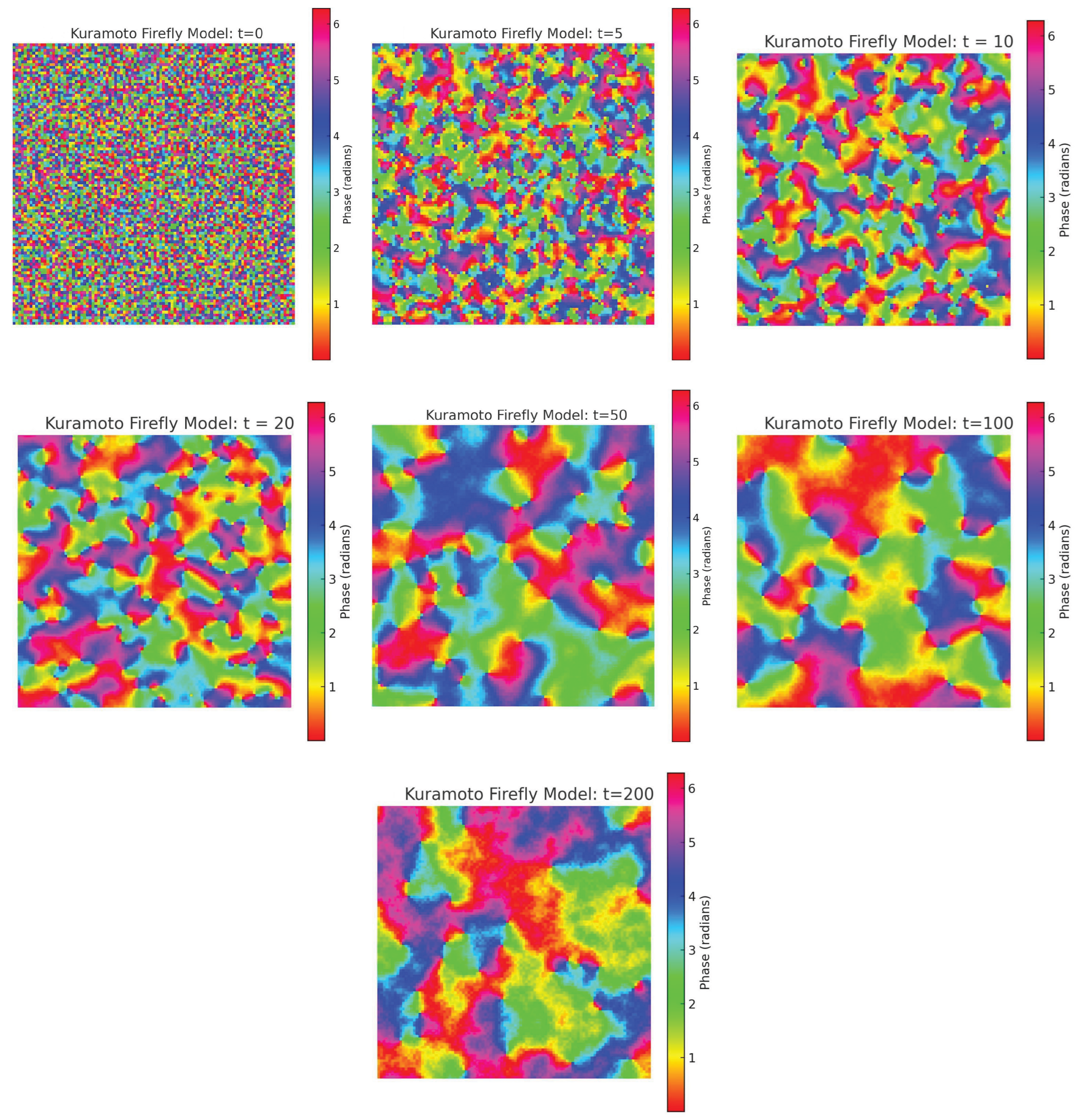
12. Ising Model

12.1. Governing Equation

We propose the following discrete evolution equation for the well-known Ising Model [13]:

$$\begin{array}{cc}\hfill E_{t}u=& \left(1-\delta \left(sign\left(J{S}_{V}u\right)-sign\left(u\right)\right)\right)\theta (F-\epsilon )sign\left(J{S}_{V}u\right)\hfill \\ \hfill & +\delta \left(sign\left(J{S}_{V}u\right)-sign\left(u\right)\right)\theta (F-F_0)\left(-sign\left(J{S}_{V}u\right)\right)\hfill \end{array}$$

(1)

where

$$S_{V}u=\sum _{(i,j)\in V}{E}_x^i{E}_y^{j}u,$$

• V is the von Neumann neighbourhood.
• $u=u(t,x,y)\in \{-1,+1\}$ is the binary state at discrete time t and spatial coordinate $(x,y)$.
• $E_{t}u:=u(t+1,x,y)$ is the next time step value.
• $F=F(t,x,y)\sim \mathcal{N}(\mu ,c^2)$ is a random driving field at site $(x,y)$, drawn from a normal distribution centered at $\mu =kT$, where T is the temperature and k is a constant.
• $\epsilon$ is a small positive number (baseline activation threshold).
• $F_0$ is a larger threshold required for flipping a stable site.
• J is the coupling constant determining interaction strength between neighbouring sites.

12.2. Physical Interpretation

The function $u(t,x,y)$ represents the spin (or state) of a particle or site at position $(x,y)$ and time t. The variable $E_{t}u$ denotes the updated state at time $t+1$. The update is governed by local interactions and stochastic environmental drive F.

• The first term activates when the site’s current state is different from the local neighbourhood majority ($sign\left(J{S}_{V}u\right)\ne sign\left(u\right)$), allowing it to flip easily when $F>\epsilon$.
• The second term activates when the site’s current state matches the neighbourhood majority, but may still flip if the driving force exceeds a higher threshold $F_0$, modeling thermal noise or instability.

This model expresses the Ising-like behaviour in the language of partial difference equations (P$\Delta$E), linking local deterministic update rules with stochastic driving force under thermal control.

13. Greenberg–Hastings Model

13.1. Greenberg-Hastings Equation

We propose the following formulation of the Greenberg–Hastings model [14] as a partial difference equation (P$\Delta$E):

$$E_{t}u=\theta (u-1)·{\mathrm{mod}}_n(u+1)+\delta \left(u\right)·\theta (S-b)$$

where

$$S=\sum _{(i,j)\in N}\delta \left(E_x^i{E}_y^{j}u-1\right)$$

with the following definitions:

• $u=u(t,x,y)\in \mathbb{Z}$, a discrete function defined on space-time: $u:{\mathbb{Z}}^3\to \mathbb{Z}$.
• $\theta \left(x\right)=\left\{\begin{array}{cc}1,\hfill & x\ge 0\hfill \\ 0,\hfill & x<0\hfill \end{array}\right.$ is the Heaviside step function.
• $\delta \left(x\right)=\left\{\begin{array}{cc}1,\hfill & x=0\hfill \\ 0,\hfill & x\ne 0\hfill \end{array}\right.$ is the Kronecker delta function.
• ${\mathrm{mod}}_n\left(x\right)=x-n·⌊{\displaystyle \frac{x}{n}}⌋$ is the modulo-n operation.
• $n\in \mathbb{N}$ is the number of discrete states (typically $n\ge 3$).
• $b\in \mathbb{N}$ is the excitation threshold.
• N is the set of relative spatial coordinates in the neighbourhood (e.g., von Neumann or Moore).

13.2. Explanation

The Greenberg–Hastings model is a classical excitable medium model capable of producing complex spatiotemporal patterns such as spiral waves. Traditionally, it is expressed using state variables $x_{i,j}^n$ updated via nested if-else rules.

In this work, we reformulate the model as a partial difference equation (P$\Delta$E) using evolution operators and logical functions. This approach provides a more elegant, symbolic, and generalizable representation that integrates naturally into our proposed framework of discrete dynamical systems.

14. The Langton’s Ant

14.1. The Langton’s Ant Equations

We describe the classical Langton’s Ant [15] using a system of coupled ordinary and partial difference equations.

The update rules are given as follows:

$$\begin{array}{cc}\hfill u(t+1,x,y)& =u(t,x,y)+\left(1-2u(t,x,y)\right)·\delta (x-X\left(t\right))\delta (y-Y\left(t\right))\hfill \\ \hfill d(t+1)& =\left(d\left(t\right)+\left(1-2u(t,X(t),Y(t\left)\right)\right)\right)mod4\hfill \\ \hfill X(t+1)& =X\left(t\right)+cos\left({\displaystyle \frac{\pi }{2}}·d(t+1)\right)\hfill \\ \hfill Y(t+1)& =Y\left(t\right)-sin\left({\displaystyle \frac{\pi }{2}}·d(t+1)\right)\hfill \end{array}$$

Here, $\delta (·)$ denotes the Kronecker delta function:

$$\delta \left(x\right)=\left\{\begin{array}{cc}1\hfill & \mathit{if}x=0\hfill \\ 0\hfill & \mathrm{otherwise}\hfill \end{array}\right.$$

The above equations can be rewritten in operator form as:

$$\begin{array}{cc}\hfill E_{t}u& =u+(1-2u)·\delta (x-X)\delta (y-Y)\hfill \\ \hfill E_{t}d& ={\mathrm{mod}}_4\left(d+(1-2u(t,X,Y\left)\right)\right)\hfill \\ \hfill E_{t}X& =X+cos\left({\displaystyle \frac{\pi }{2}}·E_{t}d\right)\hfill \\ \hfill E_{t}Y& =Y-sin\left({\displaystyle \frac{\pi }{2}}·E_{t}d\right)\hfill \end{array}$$

where:

• $u=u(t,x,y)\in \{0,1\}$ is the state of the lattice at time t and position $(x,y)$, i.e., $u:{\mathbb{Z}}^3\to \{0,1\}$.
• $d=d\left(t\right)\in \{0,1,2,3\}$ is the direction of the ant at time t, where $d:\mathbb{Z}\to {\mathbb{Z}}_4$.
• $(X\left(t\right),Y\left(t\right))\in {\mathbb{Z}}^2$ is the location of the ant, with $X,Y:\mathbb{Z}\to \mathbb{Z}$.
• The modulo function is defined as: ${\mathrm{mod}}_4\left(x\right)=x-4·⌊{\displaystyle \frac{x}{4}}⌋$.

This is a system of coupled difference equations consisting of:

• One partial difference equation for the lattice state $u(t,x,y)$.
• Three ordinary difference equations for the ant’s direction and position: $d\left(t\right)$, $X\left(t\right)$, and $Y\left(t\right)$.

14.2. Observations and Phenomena

The following figure illustrates the evolution of Langton’s Ant over discrete time steps.

The system exhibits transient chaos, followed by the emergence of a repeating structure called the highway, which acts as a periodic attractor in the phase space.

15. The Discrete Parallel Universe of PDE

15.1. Motivation

In the course of formulating a wide class of complex systems using Partial Difference Equations (P$\Delta$E), we observed that their resemblance to Partial Differential Equations (PDE) goes far beyond the multivariable function structure.

Figure 13. The evolution of Langton’s Ant over time. The black squares represent flipped cells (state 1), the white background denotes unvisited cells (state 0), and the red dot indicates the current position of the ant at the final time step.

Figure 13. The evolution of Langton’s Ant over time. The black squares represent flipped cells (state 1), the white background denotes unvisited cells (state 0), and the red dot indicates the current position of the ant at the final time step.

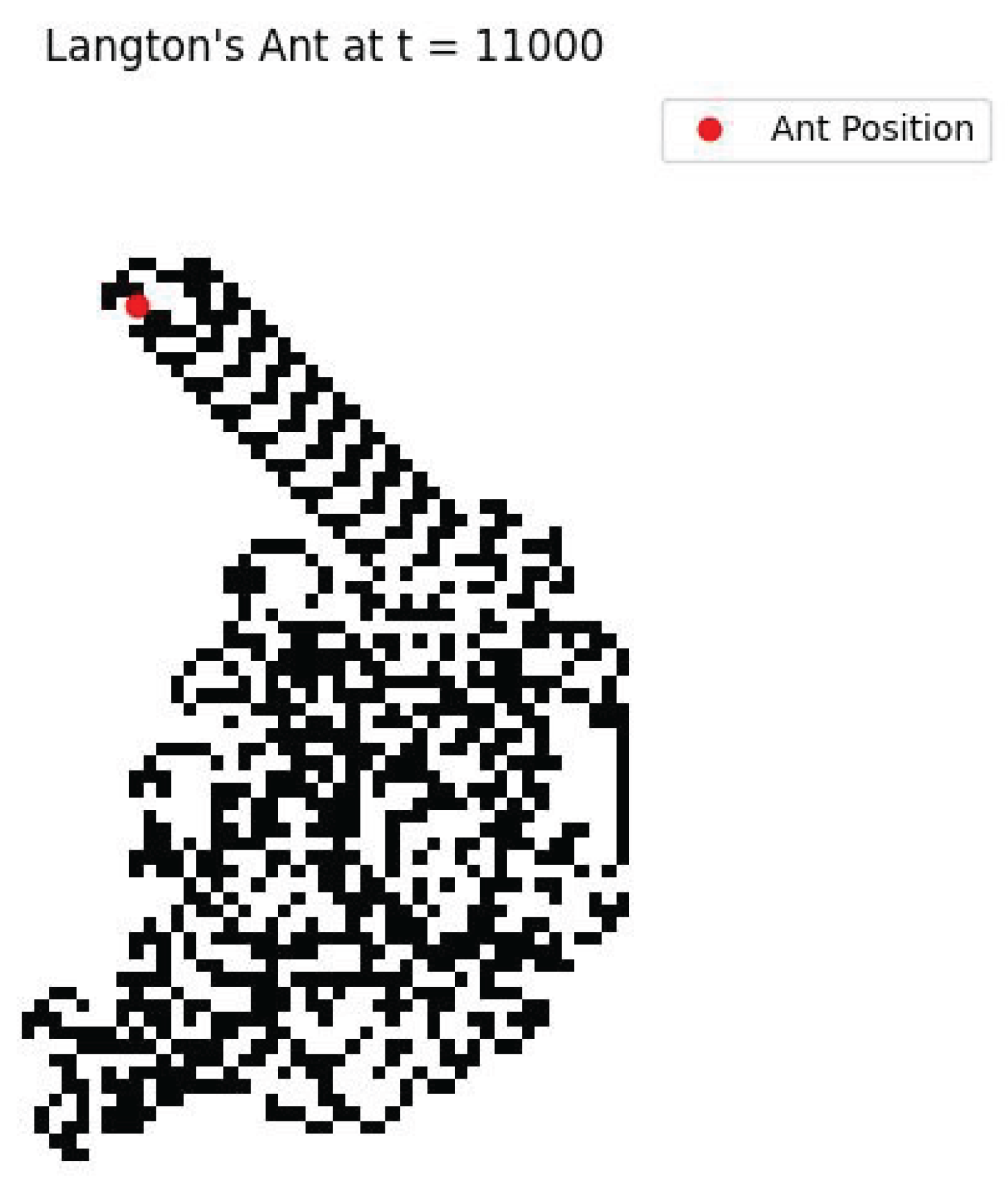
Specifically, we found deep analogies between the two worlds in terms of topology, geometry, symmetry, function spaces, algebraic structure, and even connections to number theory and combinatorics.

These similarities are not superficial; they suggest a profound duality between the continuous and the discrete, a kind of “mirror universe” where the traditional PDE-based framework has a structurally equivalent counterpart in the discrete domain.

This section aims to articulate and formalize these analogies by providing a systematic comparison between PDE and P$\Delta$E across multiple mathematical domains.

15.2. Calculus and Discrete Calculus

In the theory of Partial Differential Equations (PDE), the function u is typically a continuous multivariable function:

$$u:{\mathbb{R}}^n\to \mathbb{C}$$

In PDE, we use the differential operator, such as the partial derivative:

$${\displaystyle \frac{\partial u}{\partial t}}$$

We also use integration to accumulate values over continuous domains:

$${\int }_a^{b}f\left(x\right)dx$$

In contrast, in the theory of Partial Difference Equations (P$\Delta$E), the function u is a discrete multivariable function:

$$u:{\mathbb{Z}}^n\to \mathbb{C}$$

We use difference operators [16], such as:

$${\Delta }_{t}u=E_{t}u-u\mathrm{and}\mathrm{shift}\mathrm{operators}{E}_{t}u=u(t+1,x,\dots )$$

Instead of integrals, we use summation over discrete domains:

$$\sum _{x=a}^{b}f\left(x\right)$$

This comparison highlights the foundational parallel between classical calculus and discrete calculus, which provides the analytical tools for studying dynamics on discrete domains such as lattices or graphs.

15.3. ODE and O$\Delta$E

When we focus solely on the evolution of a single point over time, neglecting spatial structure, the continuous formulation reduces to an Ordinary Differential Equation (ODE):

$${\displaystyle \frac{du}{dt}}=f(u,t),u:\mathbb{R}\to \mathbb{C}$$

In the discrete formulation, this becomes an Ordinary Difference Equation (O$\Delta$E):

$$E_{t}u=f(u,t),u:\mathbb{Z}\to \mathbb{C},E_{t}u:=u(t+1)$$

A Partial Differential Equation (PDE) can be interpreted as an infinite system of coupled ODEs, where each spatial point evolves in time according to both its own value and its neighbours’.

Likewise, when boundary conditions are ignored, a Partial Difference Equation (P$\Delta$E) corresponds to an infinite system of coupled O$\Delta$Es, one for each spatial site on the discrete lattice.

This perspective emphasizes the structural parallelism between the continuous and discrete dynamical systems, revealing how local update rules (whether differential or difference-based) can form complex global behaviour through coupling.

15.4. Initial and Boundary Conditions

In the theory of Partial Differential Equations (PDE), the initial condition is typically given as a continuous function. For example:

$$u(0,x)=f\left(x\right),f\in C^1\left(\mathbb{R}\right)$$

The boundary [6] of the spatial domain is usually a smooth curve, surface, or differentiable manifold. Boundary conditions can be classified into:

• Dirichlet condition: Specifies the value of the function at the boundary.
• Neumann condition: Specifies the value of the normal derivative at the boundary.
• Robin condition: Specifies a linear combination of the function and its derivative at the boundary.

In contrast, for Partial Difference Equations (P$\Delta$E), the initial condition is defined as a discrete function. For instance:

$$u(0,x)=f\left(x\right),f:\mathbb{Z}\to \mathbb{C}$$

The spatial domain is defined over a lattice or graph structure, and the boundary may be a polygon (in 2D), a polyhedron (in 3D), or a higher-dimensional network.

P$\Delta$E can also incorporate discrete analogues of classical boundary conditions:

• Discrete Dirichlet condition: Specifies function values on the boundary nodes.
• Discrete Neumann condition: Specifies discrete gradients (differences) at the boundary.
• Discrete Robin condition: Specifies a linear relation between function value and difference at the boundary.

This parallel between continuous and discrete formulations illustrates the structural correspondence between PDE and P$\Delta$E in the treatment of initial and boundary data.

15.5. Laplace Transform and Z Transform

In the theory of continuous differential equations, the Laplace transform [17] is a powerful tool for solving linear ordinary or partial differential equations, particularly with constant coefficients and initial conditions. It is defined as:

$$\mathcal{L}\left[f\left(t\right)\right]=F\left(s\right)={\int }_0^{\infty }{e}^{-st}f\left(t\right)dt$$

where $f\left(t\right)$ is a continuous function defined on $[0,\infty )$, and $s\in \mathbb{C}$ is the complex frequency parameter. The Laplace transform converts a differential equation into an algebraic equation in the s-domain, which can then be solved more easily.

In contrast, in the discrete setting of difference equations, the corresponding transform is the Z-transform [5], which is used to solve linear recurrence relations and difference equations. It is defined as:

$$\mathcal{Z}\left[f\left(n\right)\right]=F\left(z\right)=\sum _{n=0}^{\infty }f\left(n\right)z^{-n}$$

where $f\left(n\right)$ is a discrete function defined on ${\mathbb{Z}}_{\ge 0}$, and $z\in \mathbb{C}$ is the complex variable. Like the Laplace transform, the Z-transform converts difference equations into algebraic equations in the z-domain.

Both transforms play analogous roles in their respective settings: converting dynamical equations into algebraic equations, enabling the application of tools from complex analysis, control theory, and systems theory.

15.6. Fourier Transform and Discrete Fourier Transform

In the theory of partial differential equations (PDE), Fourier series and the Fourier transform [6] are fundamental tools used to analyze and solve linear PDE, especially with periodic or infinite domain conditions. These methods decompose functions into sums or integrals of sinusoidal components, revealing their frequency content.

Fourier Series (Continuous, Periodic)

For a function $f\left(x\right)$ defined on a finite interval $[0,L]$, the Fourier series is given by:

$$f\left(x\right)=\sum _{n=-\infty }^{\infty }{\widehat{f}}_n{e}^{i{\displaystyle \frac{2\pi n}{L}}x}\mathrm{where}{\widehat{f}}_n={\displaystyle \frac{1}{L}}{\int }_0^{L}f\left(x\right)e^{-i{\displaystyle \frac{2\pi n}{L}}x}dx$$

Fourier Transform (Continuous, Aperiodic)

For a non-periodic function $f\left(x\right)\in L^2\left(\mathbb{R}\right)$, the Fourier transform is defined as:

$$\widehat{f}\left(\xi \right)={\int }_{-\infty }^{\infty }f\left(x\right)e^{-2\pi i\xi x}dx\mathrm{with}\mathrm{inverse}f\left(x\right)={\int }_{-\infty }^{\infty }\widehat{f}\left(\xi \right)e^{2\pi i\xi x}d\xi$$

These tools convert differential operators into algebraic ones in the frequency domain, enabling elegant solutions to linear PDE.

In the discrete setting of partial difference equations (P$\Delta$E), we have analogous tools: the Discrete Fourier Series (DFS) and the Discrete Fourier Transform (DFT) [18], which serve the same purpose in analyzing spatially discrete, periodic functions.

Discrete Fourier Series

Let $f\left[n\right]$ be a periodic discrete function defined on $n=0,1,\dots ,N-1$, then:

$$f\left[n\right]=\sum _{k=0}^{N-1}\widehat{f}\left[k\right]e^{2\pi ikn/N}\mathrm{where}\widehat{f}\left[k\right]={\displaystyle \frac{1}{N}}\sum _{n=0}^{N-1}f\left[n\right]e^{-2\pi ikn/N}$$

Discrete Fourier Transform (DFT)

The DFT is the same as DFS in form but used for numerical computation on finite-length signals:

$$\mathcal{F}{\left[f\right]}_k=\sum _{n=0}^{N-1}f\left[n\right]e^{-2\pi ikn/N}\mathrm{with}\mathrm{inverse}f\left[n\right]={\displaystyle \frac{1}{N}}\sum _{k=0}^{N-1}\mathcal{F}{\left[f\right]}_k{e}^{2\pi ikn/N}$$

These transforms diagonalize linear, shift-invariant operators and are especially useful in solving linear P$\Delta$E with constant coefficients and periodic boundary conditions.

15.7. Discrete and Continuous Green’s Function

For simplicity, we only consider the one-dimensional case.

Let $u=u(t,x)$, where $u:{\mathbb{R}}^2\to \mathbb{R}$, and consider a linear partial differential equation (PDE) of the form

$$L\left(u\right)=0,$$

where L is a linear operator. Suppose the initial condition is given by

$$u(0,x)=\delta \left(x\right),$$

where $\delta \left(x\right)$ is the Dirac delta function, and assume there are no boundary conditions. If the solution to this PDE is denoted by $G(t,x)$, the Green’s function [6], then the solution corresponding to an arbitrary initial condition $u(0,x)=f\left(x\right)$ is given by the convolution:

$$u(t,x)={\int }_{-\infty }^{\infty }f\left(s\right)G(t,x-s)ds.$$

Now, let $u=u(t,x)$, where $u:{\mathbb{Z}}^2\to \mathbb{R}$, and consider a linear partial difference equation (P$\Delta$E) of the form

$$L\left(u\right)=0,$$

where L is again a linear operator. Suppose the initial condition is

$$u(0,x)=\delta \left(x\right),$$

where $\delta \left(x\right)$ is now the Kronecker delta function, and assume there are no boundary conditions. If the solution is denoted by $G(t,x)$, the discrete Green’s function, then for an arbitrary initial condition $u(0,x)=f\left(x\right)$, the solution is given by the discrete convolution:

$$u(t,x)=\sum _{s\in \mathbb{Z}}f\left(s\right)G(t,x-s).$$

In the continuous setting, the Green’s function representation of the solution involves an integral over the spatial domain. In the discrete setting, the corresponding representation is given by a summation. These two formulations are structurally analogous, differing only in the underlying measure, Lebesgue measure for the continuous case, and counting measure for the discrete case.

15.8. Gaussian Distribution and Combinatorics

In the continuous heat equation, the equation is given by

$${\displaystyle \frac{\partial u}{\partial t}}=\alpha {\displaystyle \frac{{\partial }^{2}u}{\partial x^2}}.$$

Consider the initial condition

$$u(0,x)=\delta \left(x\right),$$

where $\delta \left(x\right)$ is the Dirac delta function. With no boundary condition, the solution is

$$u(t,x)={\displaystyle \frac{1}{\sqrt{4\pi \alpha t}}}exp\left(-{\displaystyle \frac{x^2}{4\alpha t}}\right),$$

which is the Gaussian distribution.

In the discrete heat equation, the equation becomes

$${\Delta }_{t}u=\alpha {\nabla }^{2}u,$$

and choosing $\alpha ={\displaystyle \frac{1}{2}}$, we write the equation as

$$E_{t}u={\displaystyle \frac{1}{2}}\left(E_{x}u+E_x^{-1}u\right).$$

Consider the initial condition

$$u(0,x)=\delta \left(x\right),$$

where $\delta \left(x\right)$ is the Kronecker delta function, and again, no boundary condition is imposed.

Then the solution is given by

$$u(t,x)=\delta \left({mod}_2(x+t)\right)·C\left(t,{\displaystyle \frac{x+t}{2}}\right)·{\left({\displaystyle \frac{1}{2}}\right)}^t,$$

where

$$C(n,k)=\left\{\begin{array}{cc}{\displaystyle \frac{n!}{k!(n-k)!}}\hfill & \mathit{if}0\le k\le n,\hfill \\ 0\hfill & \mathrm{otherwise}.\hfill \end{array}\right.$$

We can see that the Gaussian distribution is closely related to combinatorics. In fact, the Gaussian distribution emerges as the continuous limit of the binomial distribution as the number of trials tends to infinity, with appropriate scaling and centering, a consequence of the Central Limit Theorem.

15.9. Discrete and Continuous Dynamical Systems

In the framework of topological dynamics, a dynamical system is defined as a pair $(X,{\phi }^t)$, where X is a topological space called the state space, and ${\phi }^t:X\to X$ is a family of time-evolution operators indexed by $t\in T$, where $T=\mathbb{R}$ (continuous time) or $T=\mathbb{Z}$ (discrete time). The map ${\phi }^t$ satisfies the semigroup property ${\phi }^{t+s}={\phi }^t\circ {\phi }^s$ and ${\phi }^0=\mathrm{id}$ [19].

Continuous Dynamical Systems.

Partial Differential Equations (PDE) define continuous dynamical systems, typically of the form:

$$u:{\mathbb{R}}^n\to \mathbb{C},\mathrm{e}.\mathrm{g}.,u(t,x,y,z),\mathrm{with}t\in \mathbb{R},(x,y,z)\in \Omega \subseteq {\mathbb{R}}^3.$$

The state space X is a continuous function space, such as $L^2(\Omega )$, $C^k(\Omega )$, or Sobolev spaces $H^k(\Omega )$. The evolution of the system is governed by differential operators that act on these function spaces. In such systems, chaotic behaviour is rare and usually manifests as smooth strange attractors—continuous curves resembling vortices or spirals. The attractors tend to be geometrically regular and topologically simple.

Discrete Dynamical Systems.

Partial Difference Equations (P$\Delta$E) define discrete dynamical systems, where

$$u:{\mathbb{Z}}^n\to \mathbb{C},\mathrm{e}.\mathrm{g}.,u(t,x,y,z),\mathrm{with}t\in \mathbb{Z},(x,y,z)\in \Omega \subseteq {\mathbb{Z}}^3.$$

The state space X is a discrete function space, i.e., a space of functions defined on a lattice, often taking values in $\mathbb{C}$, $\mathbb{Z}$, or even a finite set (such as Boolean values), for example, discrete Hilbert Space: ${\mathcal{L}}^2(\Omega )$. Such systems are capable of generating highly complex spatiotemporal patterns and exhibit rich chaotic behaviours. The associated strange attractors can have fractal geometries far more exotic than in continuous systems: they may resemble turbulent flows, ribbons, spider webs, tunnels, wings, bottles, or other intricate structures.

Fractals and Complexity.

Fractals are rarely seen in PDE due to the smoothness constraints imposed by the function space and differential operators. In contrast, P$\Delta$E can easily generate fractal structures. For example:

• Rule 90 cellular automaton generates the Sierpiński triangle.
• The Abelian Sandpile Model exhibits discrete self-organized criticality with fractal avalanche clusters.
• Coupled Map Lattices generate chaotic spatial patterns with complex attractors.

These observations suggest that discrete dynamical systems possess a fundamentally different character compared to continuous ones: their state spaces are inherently combinatorial, their attractors more irregular, and their emergent behaviours often more computationally universal and structurally complex.

15.10. Manifolds and Networks

Partial Differential Equations (PDE) are traditionally defined on smooth manifolds [20], such as curves, surfaces, or general Riemannian manifolds. The underlying space is continuous, and thus the study of PDE often requires tools from differential geometry. PDE can be formulated in various coordinate systems, including rectangular, cylindrical, and spherical coordinates, depending on the geometry of the manifold.

In contrast, we observe that Partial Difference Equations (P$\Delta$E) need not be confined to rectangular grids. They can also be defined on triangular lattices, hexagonal lattices, and other non-rectangular discretizations [21]. Furthermore, P$\Delta$E can be formulated on polyhedral surfaces such as Goldberg polyhedra, zonohedra, and even higher-dimensional polytopes [22]. In this case, the underlying structure is a discrete network, and the evolution takes place over this network.

The study of such discrete geometric networks naturally connects to graph theory and discrete differential geometry. Moreover, P$\Delta$E exhibit deep relationships with discrete and computational geometry.

Although PDE and P$\Delta$E belong to continuous and discrete domains respectively, the geometric structures underlying them exhibit a fascinating duality. This suggests a possible formal correspondence between smooth manifolds and discrete networks, and opens a path to unify the continuous and discrete geometric theories under a common framework.

15.11. Boolean Algebra, Theoretical Computer Science and Number Theory

In certain classes of Partial Difference Equations (P$\Delta$E), such as those arising from elementary cellular automata, the state space is restricted to two values, typically $\{0,1\}$. This naturally connects such systems to Boolean algebra, where logical operations govern the update rules. The evolution of these discrete systems is thus governed by logical expressions, and the resulting dynamics can often be described entirely in terms of Boolean functions.

Moreover, the well-known Conway’s Game of Life, which can also be viewed as a particular P$\Delta$E defined over a two-dimensional grid with binary states, is known to be Turing complete [23]. This highlights a deep and important connection between P$\Delta$E and theoretical computer science [24], as such systems are capable of universal computation. Cellular automata and related P$\Delta$E systems therefore serve as bridges between dynamical systems, logic, and computation.

Additionally, difference equations have strong ties to number theory [24]. For example, the Fibonacci sequence satisfies the recurrence relation

$$x(t+1)=x\left(t\right)+x(t-1),$$

which is a second-order linear ordinary difference equation. More generally, integer-valued solutions to linear P$\Delta$E often exhibit rich combinatorial and arithmetic structures. In many cases, the solutions involve binomial coefficients, discrete convolutions, or integer sequences catalogued in number theory. The fact that P$\Delta$E naturally accommodate integer-valued functions $u(t,x)\in \mathbb{Z}$ reinforces their relevance to number-theoretic investigations.

Hence, P$\Delta$E lie at the intersection of Boolean algebra, number theory, and computational theory, offering a unified framework for exploring discrete structures and their evolution.

15.12. Summary

We observe that although partial differential equations (PDE) and partial difference equations (P$\Delta$E) differ fundamentally in nature, one being continuous and the other discrete, they exhibit profound structural similarities, often appearing as duals of one another.

Moreover, we have seen that P$\Delta$E are deeply interconnected with various domains of discrete mathematics, including combinatorics, number theory, graph theory, and discrete and computational geometry.

Partial Difference Equations are not merely exotic multivariable recurrence relations; rather, they serve as a unifying framework that bridges numerous areas in the discrete mathematical landscape.

16. Summary

16.1. From Numerical Methods to Language of Complexity

We began this work by introducing Partial Difference Equations (P$\Delta$E) as a formal mathematical framework for modeling systems that are discrete in both time and space. Starting from their motivation and definitions, we established their relationship to ordinary difference equations (O$\Delta$E) and to their continuous counterparts, partial differential equations (PDE), thereby clarifying the scope and intent of this study.

We then examined the linear theory, presenting the main types of linear P$\Delta$E and illustrating simple analytic solutions without pursuing a full solution theory. This led naturally to the development of discrete functional analysis tools: discrete function spaces, Hilbert space structures, and discrete operators, including shift and difference operators, along with their adjoint properties. Within this setting, we defined the discrete Green’s function and demonstrated how it parallels its continuous analogue.

The unifying strength of the P$\Delta$E formalism was then illustrated by reformulating a broad spectrum of well-known discrete models, ranging from cellular automata and coupled map lattices to sandpile models, the Ising model, and beyond, into explicit P$\Delta$E form. These examples demonstrate that systems traditionally studied in isolation can be expressed within a single coherent mathematical language.

Finally, we compared the “discrete universe’’ of P$\Delta$E with the continuous universe of PDE, revealing deep structural parallels while emphasizing their distinct mathematical foundations. In this view, P$\Delta$E and PDE emerge as mathematical twins: discrete–continuous analogues that share a common formal architecture yet belong to fundamentally different domains of mathematics.

From their origins as tools in numerical methods, difference equations have evolved here into a general language of complexity, capable of describing, unifying, and extending a wide variety of models in physics, biology, and computation. This perspective not only enriches the theoretical foundations of discrete dynamical systems but also opens pathways for future research across the sciences.

References

- Murray, J. Mathematical Biology: I. An Introduction, third ed.; Vol. 17, Interdisciplinary Applied Mathematics, Springer-Verlag: New York, Berlin, Heidelberg, 2002. [Google Scholar]
- Murray, J. Mathematical Biology II: Spatial Models and Biomedical Applications, third ed.; Vol. 18, Interdisciplinary Applied Mathematics, Springer-Verlag: New York, Berlin, Heidelberg, 2003. [Google Scholar]
- Bak, P.; Tang, C.; Wiesenfeld, K. Self-Organized Criticality: An Explanation of 1/f Noise. Physical Review Letters 1987, 59, 381–384. [Google Scholar] [CrossRef] [PubMed]
- Johnston, N.; Greene, D. Conway’s Game of Life: Mathematics and Construction; Self-published, 2022; p. 492. Hardcover, colour printing; US letter size (8. [CrossRef]
- Elaydi, S. An Introduction to Difference Equations, 3rd ed.; Undergraduate Texts in Mathematics, Springer: New York, 2005. [Google Scholar]
- Olver, P.J. Introduction to Partial Differential Equations; Undergraduate Texts in Mathematics, Springer: Cham, Heidelberg, New York, Dordrecht, London, 2014. [Google Scholar] [CrossRef]
- Wolfram, S. A New Kind of Science, 1st ed.; Wolfram Media: Champaign, Illinois, 2002. [Google Scholar]
- Itoh, M.; Chua, L.O. Difference Equations for Cellular Automata. International Journal of Bifurcation and Chaos 2009, 19, 805–830. [Google Scholar] [CrossRef]
- Yanagita, T.; Kaneko, K. Coupled map lattice model for convection. Physics Letters A 1993, 175, 415–420. [Google Scholar] [CrossRef]
- Li, B.Q.; Wang, S.J. Self-Organized Criticality in an Anisotropic Earthquake Model. Communications in Theoretical Physics 2018, 69, 280–284. [Google Scholar] [CrossRef]
- Sun, X.; Li, N.; Chen, D.; Chen, G.; Sun, C.; Shi, M.; Gao, X.; Wang, K.; Hezam, I.M. A Forest Fire Prediction Model Based on Cellular Automata and Machine Learning. IEEE Access 2024, 12, 55389–55403. [Google Scholar] [CrossRef]
- Strogatz, S.H. From Kuramoto to Crawford: Exploring the Onset of Synchronization in Populations of Coupled Oscillators. Physica D: Nonlinear Phenomena 2000, 143, 1–20. [Google Scholar] [CrossRef]
- Singh, S.P. The Ising Model: Brief Introduction and Its Application. In Solid State Physics; IntechOpen, 2020. CC BY 3. [CrossRef]
- Wu, A.C.; Xu, X.J.; Wang, Y.H. Excitable Greenberg-Hastings cellular automaton model on scale-free networks. arXiv preprint cond-mat/0701248, 0701. [Google Scholar]
- Boon, J.P. Langton’s Ant as an Elementary Turing Machine. In Nonequilibrium Thermodynamics and Fluctuation Kinetics; Springer, Cham, 2022; Vol. 208, Fundamental Theories of Physics, pp. 135–140. [CrossRef]
- Mariconda, C.; Tonolo, A. Discrete Calculus: Methods for Counting; Vol. 103, UNITEXT - La Matematica per il 3+2, Springer International Publishing: Switzerland, 2016. [Google Scholar] [CrossRef]
- Adkins, W.A.; Davidson, M.G. Ordinary Differential Equations; Undergraduate Texts in Mathematics, Springer, 2012.
- Mutagi, R.N. Understanding the Discrete Fourier Transform. PDF lecture notes, 04. Uploaded by the author on ResearchGate, Indus University. 20 January.
- Brin, M.; Stuck, G. Introduction to Dynamical Systems, 1st ed.; Cambridge University Press, 2002. Graduate-level introduction to dynamical systems theory; Cambridge, 1st ed.
- Petersen, P. Riemannian Geometry, 3rd ed.; Vol. 171, Graduate Texts in Mathematics, Springer, Cham, 2016. [CrossRef]
- Devadoss, S.L.; O’Rourke, J. Discrete and Computational Geometry, 1st ed.; Princeton University Press, 2011.
- Discrete Mathematics and Its Applications, Chapman & (Ed.) Handbook of Discrete and Computational Geometry, 3rd ed.; Discrete Mathematics and Its Applications, Chapman & (Ed.) Hall/CRC: Boca Raton, FL, 2017. [Google Scholar] [CrossRef]
- Rendell, P. Game of Life Turing Machine. In Turing Machine Universality of the Game of Life; Adamatzky, A.; Martínez, G.J., Eds.; Springer International Publishing, Cham, 2016; Vol. 18, Emergence, Complexity and Computation, pp. 45–70. [CrossRef]
- Rosen, K.H. (Ed.) Handbook of Discrete and Combinatorial Mathematics, 2nd ed.; Discrete Mathematics and Its Applications, Chapman & Hall/CRC, 2017; p. 1612. [CrossRef]
Disclaimer/Publisher’s Note: The statements, opinions and data contained in all publications are solely those of the individual author(s) and contributor(s) and not of MDPI and/or the editor(s). MDPI and/or the editor(s) disclaim responsibility for any injury to people or property resulting from any ideas, methods, instructions or products referred to in the content. |
© 2025 by the authors. Licensee MDPI, Basel, Switzerland. This article is an open access article distributed under the terms and conditions of the Creative Commons Attribution (CC BY) license (http://creativecommons.org/licenses/by/4.0/).
Copyright: This open access article is published under a Creative Commons CC BY 4.0 license, which permit the free download, distribution, and reuse, provided that the author and preprint are cited in any reuse.