Submitted:
14 July 2025
Posted:
15 July 2025
You are already at the latest version
Abstract
This paper considers the possibility of using physics-informed neural networks (PINNs) to study hydrological processes of model river sections. The fully connected neural network is used for approximation of the Saint-Venant equations in both 1D and 2D formulations. The study addresses a forward problem to determine velocities and water level, discharge and area of water section in 1D case, as well as an inverse problem to calculate the roughness coefficient. To evaluate the applicability of PINN for modeling flows in channels, it seems reasonable to start with cases where exact reference solutions are available. For the 1D case the research examines a rectangular channel with given length, width, constant roughness coefficient. An analytical solution is obtained to calculate the discharge and area of water section. The 2D model examples were also examined. The synthetic data were generated in Delft3D code, which included velocity field and water level, for the purpose of PINN training. The influence of PINN hyperparameters on the prediction result was studied. Finally, the absolute error value was assessed. The prediction error of the roughness coefficient n value in 2D case for the inverse problem did not exceed 10%. The one typical training process took from 2.5 to 3.5 hours and the prediction process took 5-10 seconds using developed PINN model on server with Nvidia A100 40GB GPU.
Keywords:
channel
; section
; Saint-Venant equations
; physics-informed neural network
; analytical solution
; numerical domain
; flow
; velocity
; inverse problem
; roughness coefficient
; training process
; learning rate
; error
1. Introduction
Global climate change affects the regional climate, resulting in heavy precipitation and river flooding. Strong climatic contrasts over Europe - northern and southern air currents over 2,000 km, high temperatures in the Mediterranean region, and polar air over the North Sea - led to massive moisture transport to eastern Central Europe and intense precipitation accumulation in the Carpathian Vault and the Northern Alps. The situation was exacerbated by climate change, which caused the Mediterranean Sea to warm up and the atmosphere to absorb more moisture, leading to more prolonged precipitation. In 2024 Mediterranean surface temperatures were at record levels, reaching between 25 °C and almost 30 °C in the northern Mediterranean region in mid-September. This meant that the temperature values were in some cases well above 4 °C above the long-term average. As a result, flooding in Central and Eastern Europe began on Friday, September 13, 2024, triggered by Cyclone "Boris", which caused severe cold and precipitation across most European countries.
According to the meteorological agency of Spain, in just a few hours in a number of places in the country the amount of precipitation equivalent to an annual indicator fell at the end of October 2024. In Chiva, west of Valencia, the agency recorded at least 491 liters of rainfall per square meter. This deluge, associated with the meteorological phenomenon known as "cold fall" (an isolated depression in altitude), forced several rivers out of their channels and caused the sudden formation of massive mudflows.
Therefore, it is essential to study the hydrological processes in rivers using mathematical modeling to construct digital twins of rivers. It is important for digital twin developers to perform real-time computations. There are several recent works in this area.
Several recent studies have demonstrated the potential of digital twin systems to enhance the modeling of hydrological processes under climate change. For example, the University of Trento developed a digital twin of the Adige River Basin in Italy to account for anthropogenic changes in reservoir dynamics [1], while the Digital Twin Earth (DTE) model incorporated high-resolution Earth observation data to simulate soil moisture, precipitation, and river discharge for improved flood forecasting [2].
A national scale model for Denmark was also introduced to function as a real-time digital twin for flood risk prediction and agricultural planning under climate extremes. The so-called GEUS, Denmark system delivered 5 terabytes of hydrological model data to the portal, with robust calibration methods and hybrid machine learning being key parts [3].
The article of authors from UK Center for Ecology and Hydrology, Lancaster, UK, reflects on the role of data science in digital twins of the natural environment, with particular attention on how resultant data models can work alongside the rich legacy of process models that exist in this domain. The authors seek to unravel the complex two-way relationship between data and understanding of processes [4].
From a mathematical point of view, the problems of studying flood processes can be reduced to solving forward and inverse problems in the field of hydrological processes using the equations of Shallow Water Theory [5].
Physics-Informed Neural Networks (PINNs), a key component of digital twins, enable real-time calculations and have been the subject of significant recent advancements [6,7,8]. PINNs embed the residual of partial differential equations (PDE) in the loss function of the neural network. They have been used successfully to solve various forward and inverse PDE problems [9,10,11].
The modern theory of solving inverse problems for hyperbolic equations is covered in the works of the authors [12,13]. Some early work in the field of numerical solutions of inverse problems in the field of hydrology is known [14,15] using various mathematical methods to solve the Saint-Venant equations [13,16,17].
Earlier research was also carried out to investigate the possibilities of using PINNs for solving hydrological problems, in particular for approximation of the 1D equation of the shallow water theory. As a rule, model problems were considered.
Several studies by scientific groups from the USA [18,19] demonstrated that PINNs successfully assimilated various types of observation and directly solved the 1D Saint-Venant equations.
The authors performed flow simulations over a floodplain and along an open channel in several synthetic case studies. PINN performance was evaluated against analytical solutions and numerical models. The results indicated that the PINN solutions of water depth had satisfactory accuracy with assimilated limited observations.
A scientific group from Ecuador investigated the numerical solution of a 1D differential equation to predict water surface profiles in a river, as well as to estimate the so-called roughness parameter [20]. Then a real mountain river morphology, the so-called Step-pool, was studied. PINN models were implemented in the TensorFlow framework using two neural networks. Different numbers of layers and neurons per hidden layer were tested, as well as different activation functions.
A 2D model for "Dam break case" was analyzed in the Ph.D. thesis [21]. The purpose of this work was to investigate the possibility of using PINNs to approximate shallow water equations (SWE), a PDE system that simulates free-surface flow problems. A wide variety of benchmark problems, selected for both steady-state solutions and Riemann problems of increasing complexity, were examined.
Another important direction is the study of filtration in porous media, including the Darcy and Richards equations.
The PINN method was presented to solve the coupled Darcy equation and the advection-dispersion equation (ADE) and was tested in a range of Pe numbers. For coupled Darcy flow and ADE with space-dependent hydraulic conductivity and velocity fields, PINN solutions for the hydraulic head and concentration were found to agree well with numerical solutions obtained with the finite-volume method [22].
Thanks to the PINN method, the numerical results obtained in real time can be used for subsequent numerical modeling of the silting of river channels. Predicting indicators is important in preventing river pollution from sedimentation. The paper [23] proposed a comparative analysis of the PINN method and numerical simulation to estimate indicators of velocity, pressure, and density in the aquatic environment.
The partial differential equation for soil–water infiltration has been combined with the PINN-based neural network to obtain a numerical analysis of the soil–water infiltration process.
The results indicated that compared to the traditional numerical method, the proposed PINN-based method for the numerical investigation of the vertical infiltration of soil and water had a smaller error and could obtain more accurate numerical results. During vertical infiltration of water in the different soil types, the light soil was the fastest, the heavy soil the second, and the medium soil the slowest [24].
The Water Retention curves (WRCs) and Hydraulic Conductivity Functions (HCFs) are critical soil-specific characteristics necessary for modeling the movement of water in soils using the Richardson- Richards equation (RRE). Well-established laboratory measurement methods for WRCs and HCFs are usually not suitable to simulate field-scale soil moisture dynamics due to the scale mismatch. The inverse solution of the RRE must be used to estimate the WRCs and HCFs from the field-measured data. The authors [25,26] proposed a PINN framework for the inverse solution of RRE and the estimation of WRC and HCF only from volumetric measurements of water content. The proposed framework does not need initial and boundary conditions, which are rarely available in real applications.
The authors of the paper [27] investigated the application of PINNs to inverse problems in unsaturated groundwater flow. PINNs have been applied to the types of unsaturated groundwater flow problems modeled with the Richards partial differential equation and the van Genuchten constitutive model. The inverse problem has been formulated as a problem with known or measured values of the solution to the Richards equation at several spatio-temporal instances, and unknown values of the solution in the rest of the problem domain and unknown parameters of the van Genuchten model. PINNs solved inverse problems by reformulating the loss function of a deep neural network so that it simultaneously aims to match the measured data and estimate the unknown values at a set of collocation points distributed across the problem domain.
The paper [28] proposed an adaptive inverse PINN applied to different transport models, from diffusion to advection-diffusion-reaction and mobile-immobile transport models for porous materials. Once a suitable PINN was established to solve the forward problem, the transport parameters were added as trainable parameters, and the reference data were added to the cost function. It was found that, for the inverse problem to converge to the correct solution, the different components of the loss function (data mismatch, initial conditions, boundary conditions, and residual of the transport equation) need to be adaptively weighted as a function of the training iteration (epoch).
In study [29], the authors proposed a new method, gradient-enhanced physics-informed neural networks (gPINNs), to improve the accuracy of PINNs. gPINNs leverage the gradient information of the PDE residual and embed the gradient into the loss function. gPINNs were extensively tested and demonstrated their effectiveness in both forward and inverse PDE problems. The numerical results showed that gPINN performs better than PINN with fewer training points.
The paper [30] addressed the peridynamic inverse problem of determining the horizon size of the kernel function in a 1D model of a linear microelastic material. The authors explored different kernel functions, including V-shaped, distributed, and tent kernels. The paper presents numerical experiments using PINNs to learn the horizon parameter for problems in one- and two-dimensional spatial dimensions.
The use of PINN for solving SWE on the sphere in a meteorological context was proposed in [31]. PINNs have been trained to satisfy the differential equations along with the prescribed initial and boundary data, and thus can be seen as an alternative approach to solving differential equations compared to traditional numerical approaches such as finite difference, finite volume or spectral methods.
Recent studies have explored the use of PINNs and other ML-based methods for modeling climate-driven processes in PDEs, combining physical constraints with data-driven learning [6,7,8,32,33].
A new area in the development of PINN architectures is related to the direction of evolutionary deep neural networks [34,35,36,37].
Currently, there are other approaches to building the PINN architecture based on Deep Operator Neural Networks (DeepOnet) [38] and Fourier Neural Operators (FNO) [39]. But these architectures are more complicated in terms of software implementation.
The process of training neural networks requires datasets that cannot always be obtained from an experiment or laboratory. The synthetic data obtained from the physical modeling can be used for this purpose. These are artificially generated data sets that are created when real hydrological data is either not available at all or is very rare or expensive to obtain.
Many fully physics-solving and reduced physics hydrodynamic models are available in numerical codes (Delft3D [40], ParFlow [41], LISFLOOD-FP [42], WRF-Hydro [43], HEC-RAS [44]).
The synthetic data for training neural networks can be obtained using one of these open source codes.
Previously, different numerical methods have been developed to solve the Saint-Venant equation in 1D/2D formulations. Among them, the authors could emphasize the semi-implicit finite-difference method [45,46]. In the paper a simple initial boundary value problem for the shallow-water equations in one space dimension was considered [47]. The authors discretized the problem in space by the standard Galerkin finite element method on a quasiuniform mesh and temporally by the classical four-stage, fourth-order, explicit Runge–Kutta scheme.
The finite-element method was combined with the classical 4th order accurate, explicit Runge-Kutta time-stepping procedure. The authors considered the one-dimensional Shallow Water Equations in a finite channel with variable bottom topography [48].
The Delft3D modeling code is very popular among hydrologists due to the availability of open source code, pre / post processors, and a wide range of many physical models to describe hydrological processes.
The Delft3D modeling code is widely used by hydrologists due to its open source availability, pre / post processors, and broad library of physical models, and has been applied, for example, to simulate temperature stratification and ice formation in deep lakes such as Lake Teletskoye [49].
A new feasible bank erosion model was developed and successfully implemented in Delft3D software code [50]. The developed model considered physical bank erosion processes to a greater extent than previous models. Model performance was assessed by comparison with a previously reported experiment in an open-channel bend flume from a mobile bed and bank laboratory.
The performance of two widely used hydrodynamic models (2D HEC-RAS and Delft3D-flexible mesh) was compared to predict the total water level (TWL) in Delaware Bay, USA in the study [51]. Based on a previously established model configuration, the authors simulated Hurricane Sandy and Isabel that affected the Bay and caused considerable damage and economic losses. The model was then evaluated with tidal analysis, comparing observed and simulated TWL, and spatio-temporal variations of TWL were analyzed through scenario-based simulations.
The Delft3D modeling code was used to identify and select the optimal living shoreline structure for a complex inlet and bay system at Carancahua Bay, Texas [52]. To achieve this goal, an extensive array of sensors was deployed to collect hydrodynamic and geotechnical data in the field, and historical shoreline changes were assessed using image analysis. The measured data were then used to parameterize and validate the baseline Delft3D model.
In the study, the process-based modeling approach was applied to assess changes in hydrodynamics and sediment dynamics resulting from climate change and engineering scenarios [53]. 2DH numerical model based on Delft3D FM was used to describe sediment dynamics and simulate the sediment budget and patterns in SSC, and turbidity levels.
In the study [54], Sandy storylines were created to assess the compound coastal flooding on critical infrastructure in New York City under different scenarios, including the effects of climate change (in the storm and through the increase in sea level) and internal variability (variations in the intensity and location of the storm). A calibrated global hydrodynamic model based on Delft3D Flexible Mesh was used as the global tide and surge model.
The paper [55] aims to assess the impact of the high-dyke system on water level fluctuations and tidal propagation in the branches of the Mekong River. A coupled 1-D to 2-D unstructured grid using Delft3D Flexible Mesh software was developed. The results showed that the inclusion of high dykes changes the percentages of seaward outflow through the different Mekong branches and modifies the seazonal flow distribution across low- and high-flow periods.
In the study [56] three methods (structural mesh encryption, suspension mesh and nonstructural mesh) based on Delft3D were compared and the optimization scheme was applied to a real bridge project. The unstructured mesh (Delft3D Flexible Mesh) scheme was unable to capture the oscillations in the wake flow behind the bridge piers. However, the application of the optimized scheme in bridge engineering demonstrated its practical value.
The purpose of this work is to develop an effective PINN model for solving 2D forward and inverse problems on the example of hydrological processes in a model channel with a given geometric parameters using synthetic data obtained from Delft3D open source hydrological code. PINN will be used to approximate the 2D Saint-Venant equations and to predict the inverse problem of finding the roughness coefficient.
The paper is organized as follows. Section 1 contains an Introduction that provides a brief overview of the research area. Section 2 covers the Materials and Methods. These are General Mathematical model for hydrological problem (Section 2.1), Formulation of the Inverse Coefficient Problem (Section 2.2), Finite difference discretization of Saint-Venant equations (Section 2.3). Section 3 covers Neural Network Architecture and the description of the Loss Function in machine learning. Section 4 covers Regularization methods and Optimization problem. Section 5 covers Definition of the problem. These are definitions for 1D problem (Section 6.1), for 2D forward problem (Section 6.2). Section 6 covers the used approach. Section 7 covers main Results. The results of numerical computations for all types of described models and their combinations are analyzed. Section 8 covers the Discussion, where both the results obtained and the hardware implementation are discussed. In the end there are Conclusions and plans to conduct further research.
2. Materials and Methods
2.1. Mathematical Model for Hydrological Problem
The mathematical model is based on the shallow water theory equations for the 1D unsteady case and the 2D steady cases. Fluid flows, which are described within the framework of the Shallow Water Theory, are very typical in practice. These include, for example, the propagation of break waves and tidal waves in rivers, the propagation of tsunami waves, currents in the bottom of hydroelectric power plants, currents in technical constrictions and flumes, and large-scale atmospheric motions in weather prediction [57,58].
These hydrological tasks are relevant when applying models in the digital twin of the agro-landscape to calculate the parameters of water movement in irrigation and drainage canals, water movement along furrows under surface irrigation, runoff of extreme storm precipitation at the catchment scale.
The system of equations for the 1D case takes the following form:
The continuity equation:
The momentum equation:
Here t is time, x is the longitudinal coordinate along the channel, W is the area of water section, Q is the discharge, q is the lateral inflow per unit length, g is the acceleration of gravity, n is the roughness coefficient according to Manning’s formula, R is the hydraulic radius, H is the water level.
The system of equations of the Shallow Water Theory (Saint-Venant equations) that describes steady two-dimensional fluid motions in the horizontal plane has the following form.
The continuity equation for 2D flow:
The momentum equation in OX direction:
The momentum equation in OY direction:
The water level:
The channel bed surface is defined by the equation:
Here x,y are coordinates along and across the channel, h is water depth, are depth-averaged velocity components along x and y coordinates, g is acceleration of gravity, n is bed surface roughness coefficient according to Manning’s formula, mu is eddy viscosity coefficient.
The equations 3, 4, 5 express the laws of conservation of the mass of the fluid and conservation of its momentum under the condition of constant fluid density. The equations of the Shallow Water Theory can be derived, in particular, from the unsteady three-dimensional Euler or Navier-Stokes equations by the procedure of averaging along the vertical coordinate.
The numerical modeling of flows in plain river sections requires the following empirical information:
- Morphometry (Digital Elevation Model) of the river valley
- Roughness coefficient of the underlying surface
- Discharge at inlet
- Water level at outlet
The possible roughness coefficient values are shown in Table 1.
2.2. Formulation of the Inverse Problem for the coefficient problem
We have to find the unknown coefficients n or and the solutions , and that satisfy:
- The Saint-Venant equations,
- Initial and boundary conditions,
- Additional conditions (observations).
The coefficient inverse problem can be expressed as a minimization problem.
2.3. Finite difference discretization of Saint-Venant equations
We represent the derivatives in a differential equations with finite difference discretization both on a uniform grid in order to solve the differential Saint-Venant equations numerically in Delft3D.
We construct a finite difference scheme for this problem. First, let us demonstrate this scheme using a uniform grid.
In the Delft3D code, the derivative approximation is performed taking into account the use of a curvilinear coordinate system, a structured or unstructured mesh, and other important features. A detailed implementation of discretization methods can be studied by downloading the source code of the solvers from the site https://oss.deltares.nl.
In Delft3D the following advection schemes have been implemented: WAQUA-scheme; Cyclic method; Flooding-scheme; Multi-directional upwind (Z-model only).
The choice of spatial discretization of the advective terms has a great influence on the accuracy, monotony, and efficiency of the computational method. The central differences are often second-order accurate, but may give rise to nonphysical spurious oscillations, the so-called “wiggles” in the solution.
These “wiggles” arise in the vicinity of steep gradients of the quantity to be resolved. In SWE theory flow these "wiggles" may also be introduced near closed boundaries and thin dams. However, first-order upwinding is unconditionally wiggle-free or monotone, thus promoting the stability of the solution process but may introduce a truncation error, which has the form of a second-order artificial viscosity term.
Finally, in our work, we used the cyclic method for spatial discretization of advective terms [59]. We took the second derivatives with central differences, which are often second-order accurate.
The equations of continuity and motion are solved by a semi-implicit method.
3. Neural Network Architecture
In the framework of this paper, the architecture of a Fully Connected Neural Network (FCNN) is considered to construct a physically-informed neural network for modeling various simple flows. For the neural network the following concepts are introduced: an input layer with neurons with features specified at the input in the form of point coordinates and discrete time values, the several hidden layers with neurons, the output layer with neurons.
The network also incorporates initial and boundary conditions, a point cloud representing the computational domain, and a loss function based on the continuity and momentum equations.
Such a physics-informed neural network consists of three main blocks. The first part includes a module for calculating residual summands for partial differential equations or the relative error of the solution in L1-L2 norm, as well as errors for initial and boundary conditions. The parameters for the FCNN are determined by finding the minimum for the overall loss function. The inputs for the neural network are converted into corresponding outputs. The second part is a FCNN with physical data, which takes the output function’s fields and calculates their derivatives using the initial equations for motion and continuity for fluid mechanics problems. The boundary and initial conditions, as well as the observational data from the experiment, are also evaluated.
The last step is the backpropagation mechanism, which minimizes the loss function using a given optimizer (for example, Adam and L-BFGS-B) according to some learning rate to obtain the optimal parameters for the neural network.
3.1. Mathematical Model for Neural Network
In our approach, we consider a FCNN of L layers and neurons in the kth layer. The weight matrix and bias vector in the kth layer (1<k<L) are denoted by and . The input vector is indicated by and the output vector in the k th layer is indicated by and .
We denote the activation function by , which is applied layer-wise along with the scalable parameters. is responsible for the slope of activation function in each hidden-layer and thereby increasing the training speed. Such locally adaptive activation functions enhance the learning capacity of the network, especially during the early training period.
The - hidden layer of FCNN is defined as
In general, the parameterized conservation law is given by
We solve forward problems where solutions of partial differential equations are inferred given fixed model parameters as well as inverse problems, where the unknown parameters should be found from the observed or synthetic data.
The given mathematical model is converted into a surrogate model. More specifically, a given problem of solving a PDE is converted into a minimization problem where the global minimum of the loss function corresponds to the solution of the PDE. The loss function can be defined using training data points like initial and boundary conditions and the residual of the given PDE.
The main hyperparameters for the PINN are the following:
- The number of layers and neurons is shown in Table 2.
- The function of activation: tanh
- The optimizers are Adam and L-BFGS on different stages for improving convergence
- The final number of points are: num domain = 500, num boundary = 200
- The number of random method points =10000
- The kernel initializer for the weights in a neural network: Glorot uniform
- Taking into account the characteristic scales, the weighting coefficients were set equal to 1
The final number of points in the calculation domain was chosen on the basis of the predicted water surface level values obtained and the available RAM on the Nvidia GPU card.
Increasing the number of points resulted in a significant increase in training time without a noticeable improvement in accuracy and a decrease in the stability of calculations. Reducing the number of points resulted in a significant difference compared to synthetic data. The simplest example of a FCNN for PINN is shown in Figure 1.
3.2. The Loss Function Value
The loss function value is formed by summation of 3 components of errors for residuals of equations, boundary and initial conditions. The MSE metric is used to calculate the error.
The loss function for the 1D model is:
Here is the loss function for the equations, is the loss function for the boundary conditions, is the loss function for the initial conditions, is the dimensionless residual of the i-th equation at the n-th point, is the number of points inside the computational domain, , , are the number of points at inlet, at outlet and for the initial conditions, , , are the specified values of the discharge and the area of water section in the boundary and initial conditions, , are the weights also used for non-dimensionalization.
The loss function for the 2D model is:
Here is the loss function for the equations, is the loss function for the boundary conditions, is the dimensionless residual of the i-th equation at the n-th point, is the number of points inside the computational domain, , are the number of points at inlet and at outlet, , , are specified values of velocities and depth in boundary conditions, , are the weights also used for non-dimensionalization.
Similarly, MSE values are calculated for the values of the magnitude functions at the boundaries of the computational domain and at the initial moment of time.
To approach the true solution, PINNs embed the PDEs into their loss function.
The neural network was also used to solve the inverse problem - finding the roughness coefficient n. It turned out to be most effective to use the new value as the desired variable and to restore the roughness coefficient n after the solution.
Since a variant of Newton’s method is used in the solution process, it is intuitively clear that calculating the derivative of a linear function is preferable. Morever, enters the equations linearly.
The main approaches and parameters of the results presented in the further presented solutions of problems using PINN methods are given in the Table 3.
The description of approximation theory and error analysis for PINNs has been cited in the article [60] with Theorem that showed that feed-forward neural nets (FNNs) with enough neurons could simultaneously and uniformly approximate any function and its partial derivatives.
4. Regularization Methods and Optimization problem
In machine learning, a loss function quantifies how well a model’s predictions match the actual data. The goal is to minimize the loss to improve the accuracy of the model. Regularization is used to prevent overfitting by adding a penalty term to the loss function.
4.1. L1 Regularization (Lasso)
L1 regularization adds the sum of absolute values of model parameters:
Encourages sparsity, making some coefficients exactly zero.
4.2. L2 Regularization (Ridge)
L2 regularization adds the sum of squared values of model parameters:
This prevents large weights and reduces the complexity of the model.
4.3. Elastic Net Regularization
A combination of regularization of L1 and L2:
It combines the benefits of both methods.
4.4. Optimization Problem
The core problem in machine learning is parameter estimation. This requires solving an optimization problem, where we try to find the values for a set of variables , that minimize a scalar-valued loss function or cost function.
This equation represents an optimization problem commonly used in machine learning and statistics.
- — a vector of parameters of the model that we want to optimize (e.g., weights of a neural network).
- — the loss function that measures how well the model performs for a given . A lower value indicates better performance.
- — the argument of the minimum; it denotes the value of that minimizes the loss function.
- — the optimal value of the parameters that minimizes the loss function.
In simple terms, this equation expresses the process of finding the best model parameters that result in the lowest possible loss.
This equation represents a single step of the gradient descent optimization algorithm.
- represents the parameter values at the current iteration n. is the set of all weight matrices and bias vectors in the neural network. The updated parameter values for the next iteration are denoted as .
- is the learning rate, a small positive scalar that controls the step size of the update.
- represents the gradient of the loss function with respect to the parameters . It indicates the direction of the steepest ascent.
Since the gradient points in the direction of increasing the loss, multiplying it by ensures that the parameters are updated in the direction of decreasing the loss. This helps the model to converge to an optimal solution.
We usually minimized the loss function by gradient-based optimizers such as gradient descent, Adam, and L-BFGS. We noted that for smooth PDE solutions, L-BFGS could find a good solution with fewer iterations than Adam, because L-BFGS used second-order derivatives of the loss function, while Adam relied only on first-order derivatives [61]. However, for stiff solutions L-BFGS was more likely to be stuck at a bad local minimum.
5. Definition of the Problem
5.1. Flow in a Channel in 1D Formulation
The flow model problem in a channel in 1D formulation and the cases for which exact solutions exist have been considered. The most effective approach is that for a suitable exact solution of 1D Shallow Water Model equations it is easier to select a model channel that will fully correspond to the selected exact solution. For this purpose, we consider a steady flow in a rectangular channel of width D with a constant roughness coefficient n and specified strictly positive values of the water discharge
and a constant area of water section
5.2. Flow in a Channel in 2D Formulation
We considered a 2D stationary flow in a rectangular channel of length L, width B with discharge Q at inlet and water level H at outlet. The computational domain is shown in Figure 2. The bed surface is shown in Figure 3.
The problem was solved under the following conditions.
6. The Used Approach
6.1. Numerical Code Delft3D
The Delft3D 4 code was used to generate data in a 2D problem. The well-established map approach for obtaining stationary solutions to 2D case on a spatial grid. A 102 x 102 spatial grid with a mesh cell of 10 m x 1 m was used. The time step was set to 60 seconds. The model time was actually 11 days. During this time, with a margin and guaranteed, the flow is established and becomes stationary, which was also separately monitored.
The solving of typical hydrological problem took about 2 minutes on workstation with one CPU core.
6.2. How the Solution Obtained in Delft3D Was Used
For the direct task, the PINN model was trained, and then (on a more detailed grid - usually 10,000 points) the actual simulation was performed. After that, the results of the PINN and Delft3D solutions were compared.
For the inverse problem of finding the roughness coefficient, the Delft3D calculation data was immediately used when training the PINN model.
7. Results
7.1. 1D Problem
The results of PINN prediction for 1D Saint-Venant equations in a rectangular channel with a length of L=1000 m for 24 hours are shown in Figs. Figure 4 and Figure 5. The problem was solved using a meshless method. The collocation points by time and coordinate were specified in the computational domain. All derivatives necessary to form the loss function were calculated using the auto-differentiation procedure within the DeepXDE scientific library. The value of the water discharge function, predicted with PINN, had the required sinusoidal shape.
The inverse problem was implemented to determine the roughness coefficient n. The initial approximation was set to be 2 times greater than the desired one. The error in the estimated roughness coefficient did not exceed 5-10%.
We chose different numbers of collocation points in the numerical domain in the range from 8000 up to 16000. What mattered to us was the total duration of training process and the available amount of RAM on the Nvidia GPU in our server. Finally, we choose the value of 10,000 points.
7.2. 2D Forward Problem
The two different approaches were used to solve the forward problem.
During training, 500 points were used for the inner area and 200 points for the boundary conditions. The increase to 2,000 internal points and 1,000 points on the borders did not improve the results, but significantly increased the training time.
The number of points in numerical domain is specified in Table 4.
Figs. Figure 6, Figure 7 show the number of collocation points in the numerical domain. The blue dots are located on the borders, and the red dots are located in the numerical domain.
In the first approach, the learning rate value lr was set to a constant value and equal to 0.0001. In the second approach, the learning rate value was varied during the training process. The first 100000 iterations were performed at lr=0.001, the next 200000 iterations were performed at lr=0.0003, the next 2400000 iterations were performed at lr=0.0001, another 800000 iterations were performed at lr=0.00003, and finally the last million iterations were performed at lr=0.00001 (Table 5).
The modeling parameters for PINN were as follows for test 2: number of neurons at each layer - 60, number of hidden layers - 6. The results of calculations using Delft3D were considered as the reference solution.
7.3. 2D Inverse Problem
A series of calculations was performed to solve the inverse problem. Figure 10, Figure 11, Figure 12, Figure 13 show comparative results of calculations on the model of the inverse PINN problem using all the data from the Delft3D calculations and the Delft3D data itself (the first variant).
The second variant of the inverse problem is closer to the use of data from the real field observations at water gauging stations. In this case, to solve the inverse problem of finding the roughness coefficient, the results of solving the forward problem using the Delft3D code are used only at the domain inlet. Another feature of this approach is the need to obtain a more or less reasonable initial approximation of the water level.
For this purpose, the forward PINN problem is solved with a constant initial approximation of the roughness coefficient, which is assumed to be 0.1 in all cases considered below.
The second variant required noticeably larger computational resources compared to the first variant. In particular, 100000 iterations were used to generate the initial approximation, and 2 million iterations were used to solve the inverse problem itself. Empirically, it was determined that it was acceptable to set the learning rate to .
Three PINN models were used in our research, with 40 neurons at each layer and 4 hidden layers (model 1), with 60 neurons at each layer and 6 hidden layers (model 2), with 80 neurons at each layer and 8 hidden layers (model 3).
The results for the loss function during the training process are presented in Figs. Figure 14, Figure 15. As can be seen, increasing the number of neurons and layers does not necessarily lead to better results. Thus, the use of "model 3" apparently leads to the need to reduce the training speed. The difference between "model 1" and "model 2" is not so great. Although "model 1" requires more iterations, the time per iteration is about 15 % less than "model 2".
The time per iteration of "model 3" is 30% higher than the time per iteration of "model 2". Note also that the value of the loss function may not correspond to the accuracy of the roughness coefficient determination. It seems that in all cases the deviation of the calculated roughness coefficient from the reference one is more influenced by the number of PINN model points in the spatial domain.
The different values of Loss function for 2D inverse problem is shown in Figure 16. The Loss function component for the value of the vertical component of the fluid velocity prediction, while the Loss function component for the boundary condition function for the velocity at the inlet of the domain made the least.
The smallest value was the Loss function component for the boundary condition function for the velocity at the inlet of the domain.
7.4. Results of regularization
All our results are obtained without using regularization. Trial tests using L1 and L2 regularization did not improve the accuracy of the results or reduce the training time. Thus, a typical inverse problem with exactly the same parameters (except for regularization) for finding the roughness coefficient without using regularization showed n=0.027, and with L1 - n=0.0292. The exact value of n=0.025.
For our specific task, the regularization L1 and L2 methods did not provide an increase in accuracy and stability to find the roughness coefficient.
8. Discussion
8.1. Selecting Optimal Hyperparameters for PINN
When PINN has been used, the number of points in a domain varied from 500 to 50000 during training. The calculations showed that increasing the number of points when using the PINN leads to a significant and disproportionate increase in the training time also due to the necessity to reduce the learning rate lr.
Currently, classical numerical methods (finite difference, finite volume, finite element methods) even for nonlinear equations use at least semi-implicit schemes which are almost linear with respect to the variables at the next time step or the next iteration. The inversion of the arising well-conditioned matrices in this case is carried out by extremely efficient methods.
When using PINN, one of the variants of optimization method (Adam or L-BFGS-B) is used to calculate the desired variables at the next iteration. The Saint-Venant equations are essentially nonlinear. In general, the stability of the iterative process is not guaranteed in this case.
Currently, when the number of points in the domain is too large, combined with a poor initial approximation and the use of automatic differentiation, the likelihood of iteration divergence becomes higher compared to classical numerical methods.
At the same time, by experiment we have found that 500 points are enough for a stable learning process. (Table 6).
At calculations with the help of the trained model at a large number of points achieves both rather small error and very fast modeling process. When using the trained model it is possible to set, for example, 10 000 points for the given problems.
The task of selecting optimal hyperparameters for a neural network is an independent scientific problem. The solution of this problem requires the use of special scientific libraries such as Ray Tune, Optuna, HyperOpt, Scikit-Optimise and additional computational resources.
8.2. Water Level Value
Analyzing Figure 7 for water level value one can notice the presence of oscillations for the results obtained with PINN. The water level numerical solution is not too high in absolute value in the case of a 2D problem. In absolute value, the values varied slightly. Changing by only 4 centimeters per 100 meters. Only 4 centimeters of change per 100 meters.
When solving nonlinear problems by iterative method, some emperical coefficients are commonly used. For example, weight coefficients and learning rate of neural network. We have chosen these emperical coefficients in such a way that we achieve convergence. Analysis of a recent publication in the field of inverse problem solving using PINNs demonstrates the similarity of approaches to selecting these coefficients [28]. The learning rate decreases during training.
The characteristic depth is m, and the characteristic velocity is . . Since all characteristic orders are close to 1, the weighting coefficients were also taken to be equal to 1.
Several studies by scientific groups from the USA [18,19] demonstrated that PINNs successfully assimilated various types of observations and directly solved the 1D Saint-Venant equations. They demonstrated PINNs were able to assimilate observations of various types and solve 1D Saint-Venant equations directly. As a result, several model problems with small dimensions in the computational domain were solved. A scientific group from Ecuador investigated the numerical solution of a 1D differential equation to predict water surface profiles in a river, as well as to estimate the so-called roughness parameter [20]. The real mountain river morphology was then studied, but only in a 1D formulation.
We solved the direct and inverse 2D problems for a channel with a length of 1000 meters using PINN.
8.3. Convergence Behavior
The paper [30] presented numerical experiments using PINNs to learn the horizon parameter for problems in one- and two-spatial dimensions. The results demonstrated the effectiveness of PINNs in solving the peridynamic inverse problem, even in the presence of challenging kernel functions. It was observed and proven that the stochastic gradient descent method is in a one-sided convergence behavior toward a global minimum of the loss function, suggesting that the true value of the horizon parameter was an unstable equilibrium point for the gradient flow dynamics of PINN.
In our work we did not use any specific kernel function, convergence behavior was always achieved using on optimization methods (Adam and L-BFGS-B).
8.4. Hardware and Software Resources
The learning (training) process for the PINN was conducted on a Dell EMC PowerEdge XE8545 server with two Intel Xeon CPUs, running OS Linux Ubuntu, with 4 Nvidia A100 GPUs, where each GPU had 40GB RAM. The software stack was based on Python, DeepXDE library, TensorFlow framework, Numpy, Matplotlib, Jupyter Notebook.
DeepXDE library allows users to conduct their own development of thematic PINN models [60]. In our case, the peculiarities of software implementation in Python were related to writing special functions to read synthetic data obtained from Delft3D code. We also needed to write a special function for solving the Saint-Venant equations.
The paper [62] aimed to assess the applicability of PINNs as a solution method for free surface flow problems over non-flat bottom. The results of PINNs for augmented SWEs (PINN-augmSWE) are presented. For all 1D cases, training process was performed with a NVIDIA A100 GPU device. Average training time was between 7 and 8 minutes for tests with "base" configuration.
Our studies have shown that during the training process with the selected parameters it was necessary to use about 18-20 GB of memory on a single Nvidia GPU A100 40GB. A typical training process for 2D case took from 2.5 to 3.5 hours. In average, prediction process took from 5 to 10 seconds.
9. Conclusions
The posed forward and inverse hydrological problems based on the Saint-Venant equations using PINNs were successfully solved for test examples. However, our results have shown that the computational costs for solving these problems are significantly higher than those of traditional approaches, even when using Nvidia GPUs.
The simulations have shown that training with a constant learning rate is inferior in efficiency to training with a variable learning rate, which should gradually decrease during the iteration process.
It seems that the creation of an automatic procedure for changing the learning rate, based on physical principles, will be extremely useful for increasing efficiency.
The novelty in our work was that using PINN, we investigated the flow in a channel with a sharply changing bottom surface, which may be more complex than in real rivers.
It is also for the first time we solved the coefficient inverse problem for the Saint-Venant equations using PINNs in 2D case. The synthetic data was obtained in the Delft3D computational code for steady problem in a long channel. Using PINNs the velocity and water level fields were obtained. The prediction error of the roughness coefficient n value in 2D case did not exceed 10%.
The most important advantage of using PINN to study hydrological processes is the small computational time for prediction. PINNs may be in demand in digital twin models that need to perform real-time computations.
Another advantage of using PINN is the ability to explore different scenarios while varying the boundary conditions to find the roughness coefficient of the river bed.
However, one disadvantage of the first generation of PINNs is that they usually have limited accuracy even with many training points, and also place high computational demands on memory resources on GPU cards.
Further research in terms of improving prediction accuracy can be related to the use of the regularization approach and in particular to the approach based on the gPINN architecture. The future work will explore problems involving more complex river channel geometries.
Another important area of work is the use of PINNs for real hydrological scenarios, which, however, will require significant efforts to improve the architecture of neural networks. We have to draw our attention to the task of selecting input features. In particular, incorporating river channel geometry is essential.
Author Contributions
Conceptualization, K.B. and S.S.; methodology, A.B.; software, K.B.; validation, S.S. and A.B.; formal analysis, K.B.; investigation, S.S.; resources, A.B.; data curation, K.B.; writing—original draft preparation, K.B.; writing—review and editing, S.S.; visualization, K.B.; supervision, S.S.; project administration, S.S.; funding acquisition, A.B. All authors have read and agreed to the published version of the manuscript.
Funding
The work was carried out with the financial support of the Ministry of Science and Higher Education of the Russian Federation (Agreement No. 075-15-2024-545 dated April 24, 2024
Data Availability Statement
The data presented in this study are available from the corresponding author on reasonable request.
Acknowledgments
Ilia Stulov from ISP RAS, Moscow has provided constructive comments to the earlier version of this manuscript.
Conflicts of Interest
The authors declare no conflicts of interest.
Abbreviations
The following abbreviations are used in this manuscript:
| PINN | Physics Informed Neural Network |
| SWE | Shallow Water Equations |
| FCNN | Fully Connected Neural Network |
| HDT | Hydrological Digital Twin |
| DTE | Digital Twin Earth |
| PDE | Partial Differential Equations |
| WRC | Water Retention curves |
| HCF | Hydraulic Conductivity Functions |
| RRE | Richardson- Richards equation |
| TWL | Total Water Level |
| SSC | Suspended Sediment Concentration |
| MSE | Mean Squared Error |
| RAM | Random Access Memory |
| GPU | Graphics Processing Unit |
References
- Morlot, M.; Rigon, R.; Formetta, G. Hydrological digital twin model of a large anthropized italian alpine catchment: The Adige river basin. J. Hydrol. 2024, 629, 130587. [CrossRef]
- Brocca, L; Barbetta, S.; Camici, S.; Ciabatta, L.; Dari, J.; Filippucci, P.; Massari, C.; Modanesi, S.; Tarpanelli, An.; Bonaccorsi, B.; Mosaffa, H.; Wagner, W.; Vreugdenhil, M.; Quast, R.; Alfieri, L.; Gabellani, S.; Avanzi, F.; Rains, D.; Miralles, D.G. ; Mantovani, S.; Briese, C.; Domeneghetti, A.; Jacob, A.; Castelli, M.; Camps-Valls, G.; Volden, E.; Fernandez, D. A Digital Twin of the terrestrial water cycle: a glimpse into the future through high-resolution Earth observations. Front. Sci. 2024, 1-2023. https://www.frontiersin.org/journals/science/articles/10.3389/fsci.2023.1190191/full. [CrossRef]
- Henriksen, H.J.; Schneider, R.; Koch, J.; Ondracek, M.; Troldborg, L.; Seidenfaden, I.K.; Kragh, S.J.; Bøgh, E.; Stisen, S. A New Digital Twin for Climate Change Adaptation, Water Management, and Disaster Risk Reduction (HIP Digital Twin). Water 2023, 15, 25. https://www.mdpi.com/2073-4441/15/1/25. [CrossRef]
- Blair, G.S.; Henrys, P.A. The role of data science in environmental digital twins: In praise of the arrows. Environmetrics 2023, 34, e2789. https://onlinelibrary.wiley.com/doi/full/10.1002/env.2789. [CrossRef]
- Kulikovskii, A.G. ; Pogorelov, N. V.; Semenov, A. Yu. Matematicheskie voprosy chislennogo resheniya giperbolicheskikh sistem uravnenii, izd. 2-e, ispravl. i dop., Fizmatlit, Moscow, 2012.
- Raissi, M.; Perdikaris, P.; Karniadakis, G.E. Physics-informed neural networks: A deep learning framework for solving forward and inverse problems involving nonlinear partial differential equations, J. Comput. Phys. 2019, 378, 686–707. [CrossRef]
- Karniadakis, G.E.; Kevrekidis, I.G.; Lu, L.; Perdikaris, P.;Wang, S.; Yang, L. Physics-informed machine learning, Nat. Rev. Phys. 2021, 3, 422–440.
- Jin, X.; Cai, S.; Li, H.; Karniadakis, G.E. NSFnets (Navier-Stokes flow nets): physics-informed neural networks for the incompressible Navier-Stokes equations. J. Comput. Phys. 2021, 426, 109951. [CrossRef]
- Lagaris, I.; Likas, A.; Fotiadis, D. Artificial neural networks for solving ordinary and partial differential equations. IEEE Trans. Neural. Netw. 1998, 9, 987–1000. [CrossRef]
- Lagaris, I.; Likas, A.; Papageorgiou, D. Neural-network methods for boundary value problems with irregular boundaries, IEEE Trans. Neural. Netw. 2000, 11, 1041–1049. [CrossRef]
- Romanov, D.E. Neural networks of inverse error propagation. Engineering journal of Don 2009, 3, 19–24.
- Kabanikhin, S. I. Inverse and ill-posed problems, Novosibirsk, Siberian scientific publishing house, 2009.
- Bellassoued, M.; Yamamoto, M. Carleman estimates and applications to inverse problems for hyperbolic systems, Tokyo, Springer Japan, 2017.
- Szymkiewicz, R. Solution of the inverse problem for the Saint Venant equations, J. Hydrol. 1993, 147, 105–120. [CrossRef]
- Takase, H. Inverse source problem related to one-dimensional Saint-Venant equation. Appl. Anal. 2022., 101, 35–47. [CrossRef]
- Bukhgeim, A.L.; Klibanov, M.V. Global uniqueness of class of multidimensional inverse problems. Soviet Math. Dokl. 1981, 24, 244–247.
- Imanuvilov, O.; Yamamoto, M. Global Lipschitz stability in an inverse hyperbolic problem by interior observations. Inverse Probl. 2001, 17, 717–728. [CrossRef]
- Feng, D.; Tan, Z.; He, Q.Z. Physics-informed neural networks of the Saint-Venant equations for downscaling a large-scale river model. Water Resour. Res. 2023, 59, e2022WR033168.
- Rosofsky. S.G.; Al Majed, H.; Huerta E.A. Applications of physics informed neural operators. Mach. Learn.: Sci. Technol. 2023, 4, 025022. [CrossRef]
- Cedillo, S., Núñez, AG.; Sánchez-Cordero, E.; Timbe, L.; E. Samaniego E.; Alvarado A. Physics Informed Neural Network water surface predictability for 1D steady state open channel cases with different flow types and complex bed profile shapes. Adv. Model. and Simul. in Eng. Sci. 2022, 9, 10 (2022). [CrossRef]
- Riccardo, A. Physics-Informed Neural Networks for Shallow Water Equations., Ph.D. thesis, Politecnico di Milano, 2022.
- He, Q.; Tartakovsky, A.M. Physics-informed neural network method for forward and backward advection-dispersion equations. Water Resour. Res. 2021, 57, e2020WR029479. [CrossRef]
- Omarova, P.; Amirgaliyev, Y.; Kozbakova, A.; Ataniyazova, A. Application of Physics-Informed Neural Networks to River Silting Simulation. Appl. Sci. 2023, 13, 11983. [CrossRef]
- Yang, Y.; Mei, G. A Deep Learning-Based Approach for a Numerical Investigation of Soil–Water Vertical Infiltration with Physics-Informed Neural Networks. Mathematics 2022, 10, 2945. [CrossRef]
- Bandai, T.; Ghezzehei, T.A. Physics-informed neural networks with monotonicity constraints for Richardson-Richards equation: Estimation of constitutive relationships and soil water flux density from volumetric water content measurements. Water Resour. Res. 2021, 57, e2020WR027642. [CrossRef]
- Bandai, T.; Ghezzehei, T.A. Forward and inverse modeling of water flow in unsaturated soils with discontinuous hydraulic conductivities using physics-informed neural networks with domain decomposition. HESS 2022, 26, 4469–4495. [CrossRef]
- Depina, I.; Jain, S.; Valsson, S.M.; Gotovac, H. Application of physics-informed neural networks to inverse problems in unsaturated groundwater flow. GEORISK 2022, 16, 21–36. [CrossRef]
- Berardi, M.; Difonzo, F.V.; Icardi, M. Inverse Physics-Informed Neural Networks for transport models in porous materials. CMAME 2025, 435, 117628. [CrossRef]
- Yu, J.; Lu, L.; Meng, X.; Karniadakis, G.E. Gradient-enhanced physics-informed neural networks for forward and inverse PDE problems. CMAME 2022, 393, 114823. [CrossRef]
- Difonzo, F.V.; Lopez, L. ; Pellegrino, S.F. Physics informed neural networks for learning the horizon size in bond-based peridynamic models. CMAME 2025, 436, 117727. [CrossRef]
- Bihloy, A.; Popovychz, R. O. Physics-informed neural networks for the shallow-water equations on the sphere. arXiv 2022, arXiv:2104.00615v3. https://arxiv.org/abs/2104.00615.
- Kashinath, K., Mustafa, M., Albert, A., Wu, J-L., Jiang, C., Esmaeilzadeh, S., Azizzadenesheli, K., Wang, R., Chattopadhyay, A., Singh, A., Manepalli, A., Chirila, D., Yu, R., Walters, R., White, B., Xiao, H., Tchelepi, H. A., Marcus, P., Anandkumar, A., Hassanzadeh, P.; Prabhat Physics-informed machine learning: case studies for weather and climate modelling. Phil. Trans. R. Soc. A. 2021, 379, 20200093. [CrossRef]
- Lu, L., Jin, P., Pang, G.; Zhang, Z.; Karniadakis, G.E. Learning nonlinear operators via DeepONet based on the universal approximation theorem of operators. Nat. Mach. Intell. 2021, 3, 218–229. [CrossRef]
- Du, Y.; Zaki, T.A. Evolutional deep neural network, Phys. Rev. E 2021, 104, 045303.
- Anderson, W.; Farazmand, M. Fast and scalable computation of shape-morphing nonlinear solutions with application to evolutional neural networks. J. Comput. Phys. 2024, 498, 112649. [CrossRef]
- Finzi, M.; Potapczynski, A.; Choptuik, M.; Wilson, A.G. A Stable and Scalable Method for Solving Initial Value PDEs with Neural Networks. arXiv 2023, arXiv:2304.14994v2. https://arxiv.org/abs/2304.14994.
- Kim, H.; Zaki, T. A. Multi evolutional deep neural networks (Multi-EDNN). arXiv 2024, arXiv:2407.12293v1. https://arxiv.org/abs/2407.12293. [CrossRef]
- Lu, L.; Meng, X.; Cai, S.; Mao, Z.; Goswami, S.; Zhang, Z.; Karniadakis, G.E. A comprehensive and fair comparison of two neural operators (with practical extensions) based on FAIR data, CMAME 2022, 393, (2022), 114778. https://www.sciencedirect.com/science/article/abs/pii/S0045782522001207. [CrossRef]
- Li, Z.; Kovachki, N.; Azizzadenesheli, K.; Liu, B.; Bhattacharya, K.; Stuart, A.; Anandkumar, A. Fourier neural operator for parametric partial differential equations. International Conference on Learning Representations (ICLR) 2021. https://openreview.net/forum?id=c8P9NQVtmnO.
- Deltares. Delft3D-FLOW User Manual. Simulation of multi-dimensional hydrodynamic flows and transport phenomena, including sediments. Version: 3.15.52614, 1 October 2017.
- ParFlow Documentation. Release 3.13.0. Jul 09, 2024.
- Bates, P.D.; Horritt, M.S.; Fewtrell T.J. A simple inertial formulation of the shallow water equations for efficient two-dimensional flood inundation modelling. J. Hydrol. 2010, 387, 33–45. [CrossRef]
- The NCAR WRF-Hydro® Modeling System Technical Description. Version 5.1.1 Originally Created: April 14, 2013 Updated: January 20, 2020. 107 p.
- Goodell, C.R. Breaking the HEC-RAS Code - A User’s Guide to Automating HEC-RAS, h2ls, 2014.
- Casulli, V. Semi-implicit finite difference methods for the two-dimensional shallow water equations. J. Comput. Phys. 1990, 86, 56–74. [CrossRef]
- Casulli, V.; Walters, R.A. An unstructured grid, three-dimensional model based on the shallow water equations. Int. J. Numer. Methods Fluids 2000, 32, 331–348. [CrossRef]
- Antonopoulos, D.C.; V.A. Dougalis, V.A.; Kounadis, G. On the standard Galerkin method with explicit RK4 time stepping for the shallow water equations. IMA J. Numer. Anal. 2019, 40, 2415–2449. [CrossRef]
- Kounadis, G.; Dougalis, V.A. Galerkin finite element methods for the Shallow Water equations over variable bottom. J. Comput. Appl. Math. 2020, 373 (2020), 112315. [CrossRef]
- Koshelev, K.; de Goede, E.; Zinoviev, A.; de Graaff, R. Modelling of Thermal Stratification and Ice Dynamics with to Lake Teletskoye, Altai Republic, Russia. Water Resour. 2021, 48, 368–377.
- Parsapour-Moghaddam, P.; Rennie, C.D.; Slaney, J.; Platzek, F.; Shirkhani, H.; Jamieson, E.; Mosselman, E.; Measures, R. Implementation of a New Bank Erosion Model in Delft3D. J. Hydrol. Eng. 2023, 149, 13206. [CrossRef]
- Muñoz, D. F.; Yin, D.; Bakhtyar, R.; Moftakhari, H.; Xue, Z.; Mandli, K.; Ferreira, C. Inter-Model Comparison of Delft3D-FM and 2D HEC-RAS for Total Water Level Prediction in Coastal to Inland Transition Zones. JAWRA 2021, 58, 34–39. [CrossRef]
- Huff, T. P.; Feagin, R. A.; Figlus, J. Delft3D as a Tool for Living Shoreline Design Selection by Coastal Managers. Front. Built Environ. 2022, 8, 926662. doi: 10.3389/fbuil.2022.926662. [CrossRef]
- Achete, F.; Van der Wegen, M.; Roelvink, J.A.; Jaffe, B. How can climate change and engineered water conveyance affect sediment dynamics in the San Francisco Bay-Delta system?. Climatic Change 2017, 142, 375–389. [CrossRef]
- Goulart, H.M.D.; Lazaro, I. B.; van Garderen, L.; van der Wiel, K.; Bars, D.L.; Koks, E.; van den Hurk, B. Compound flood impacts from Hurricane Sandy on New York City in climate-driven storylines. NHESS 2024, 24, 29–45.
- Thanh, V. Q.; Roelvink, D.; van der Wegen, M.; Reyns, J.; Kernkamp, H.; Van Vinh, G. Linh, V.T.P. Flooding in the Mekong Delta: the impact of dyke systems on downstream hydrodynamics. HESS 2020, 24, 189–212. [CrossRef]
- Liu, X.; Chen, Q.-S.; Zeng, Z.-N.; Dong, Z. Optimisation of Bridge Pier Winding Flow Numerical Simulation Scheme Based on Delft3D. Water 2024, 16, 2079. [CrossRef]
- Göttelmann, J. A spline collocation scheme for the spherical shallow water equations, J. Comput. Phys. 1999, 148, 291–298. [CrossRef]
- Layton, A.T. Cubic Spline Collocation Method for the Shallow Water Equations on the Sphere. J. Comput. Phys., 2002 179, 578–592. [CrossRef]
- Stelling, G.S.; Leendertse, J. Approximation of Convective Processes by Cyclic AOI Methods. Estuarine and Coastal Modeling 1992, 771-782. https://api.semanticscholar.org/CorpusID:123326488.
- Lu, L.; Meng, X.; Mao, Z.; Karniadakis, G.E. DeepXDE: A Deep Learning Library for Solving Differential Equations. SIAM Rev. 2021, 63, 208–228. https://epubs.siam.org/doi/10.1137/19M1274067. [CrossRef]
- Murphy, K.P. Probabilistic Machine Learning: An Introduction. Adaptive Computation and Machine Learning series. MIT Press, 2022.
- Dazzi S. Physics-Informed Neural Networks for the Augmented System of Shallow Water Equations With Topography. Water Resources Research, 2024 60, 1–22. [CrossRef]
Figure 1.
The structure of a FCNN for 2D case. X, Y coordinates of points are features. The velocity components, water level, and roughness coefficient are predicted quantities.
Figure 1.
The structure of a FCNN for 2D case. X, Y coordinates of points are features. The velocity components, water level, and roughness coefficient are predicted quantities.

Figure 2.
The computational domain.
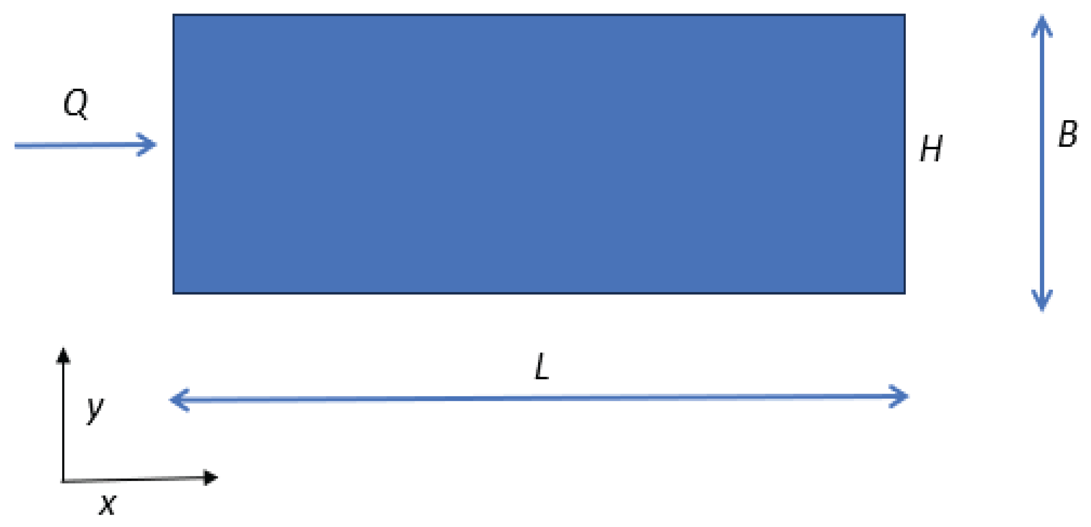
Figure 3.
The Bed surface.
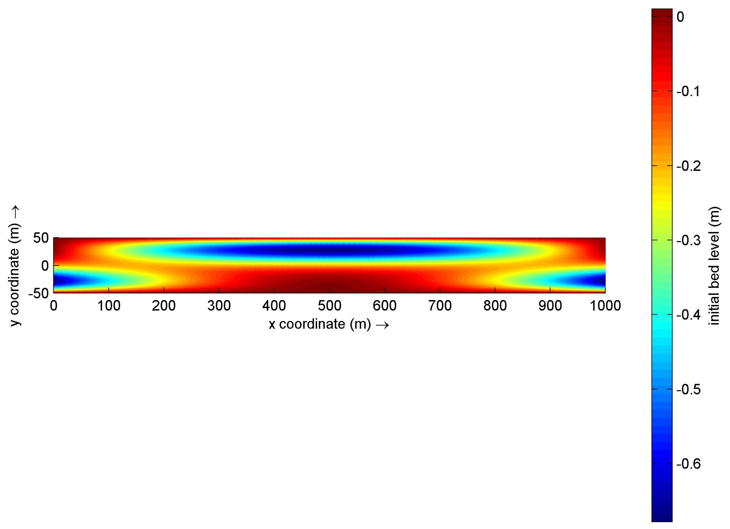
Figure 4.
The area of water section is plotted on the vertical axis. One of the horizontal axes shows the change of x coordinate, the other horizontal axis shows the dimensionless time t. 1D case.
Figure 4.
The area of water section is plotted on the vertical axis. One of the horizontal axes shows the change of x coordinate, the other horizontal axis shows the dimensionless time t. 1D case.
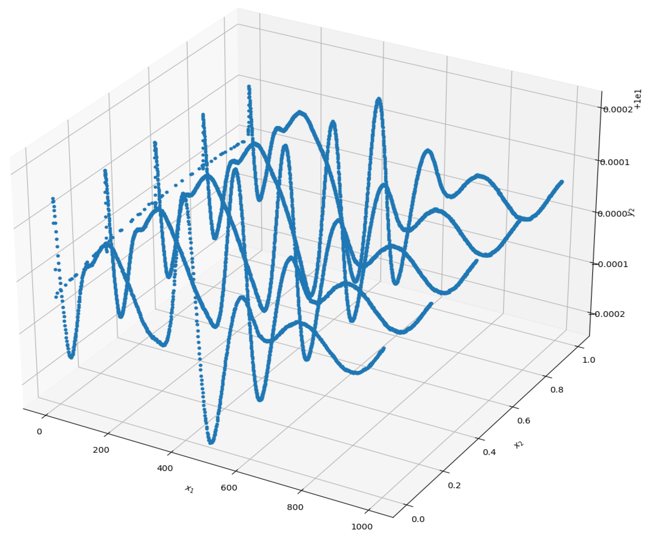
Figure 5.
The water discharge is plotted on the vertical axis. One of the horizontal axes shows the change of x coordinate, the other horizontal axis shows the dimensionless time t. 1D case.
Figure 5.
The water discharge is plotted on the vertical axis. One of the horizontal axes shows the change of x coordinate, the other horizontal axis shows the dimensionless time t. 1D case.
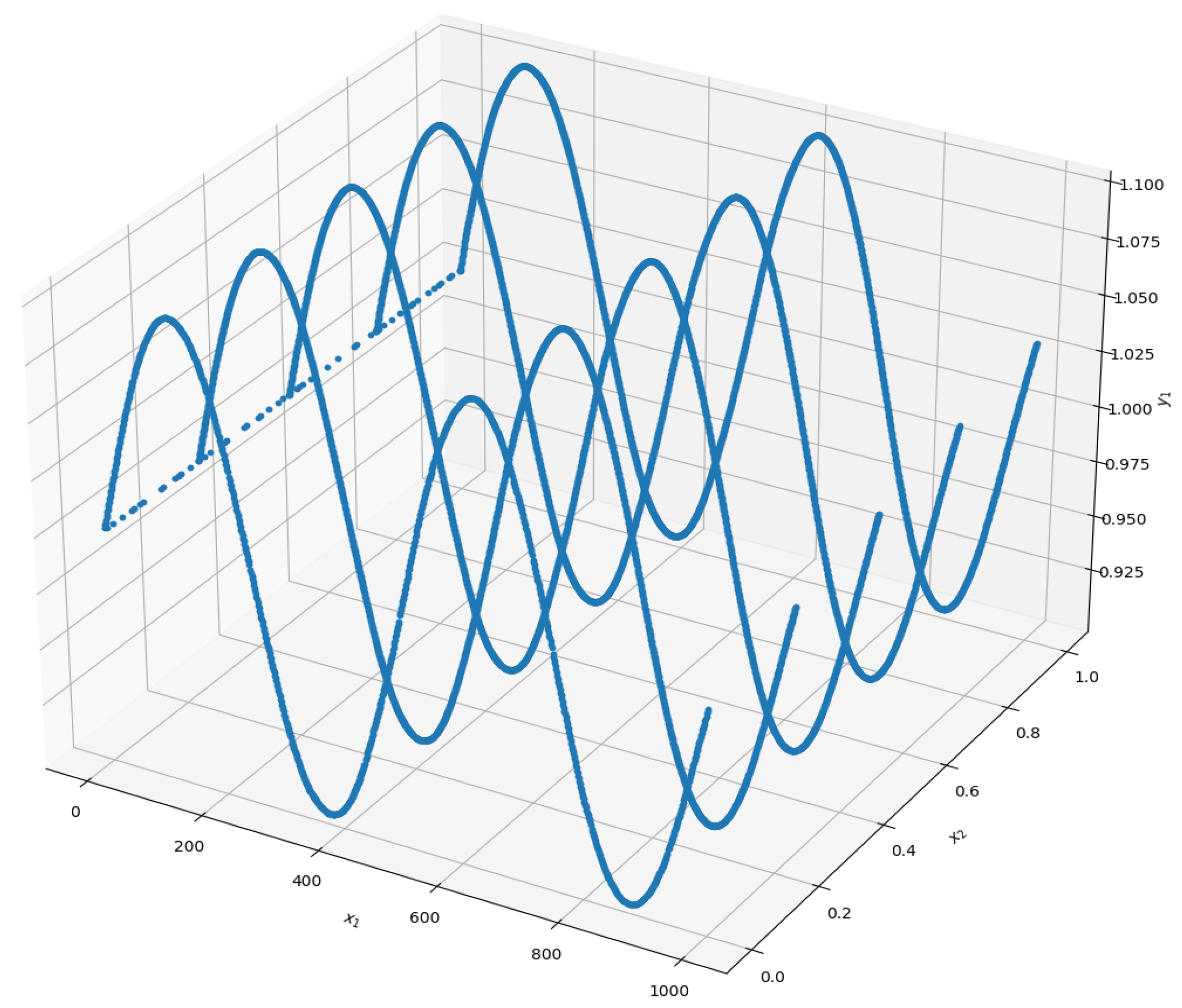
Figure 6.
The number of collocation’s points. 2D case. Grid 1.
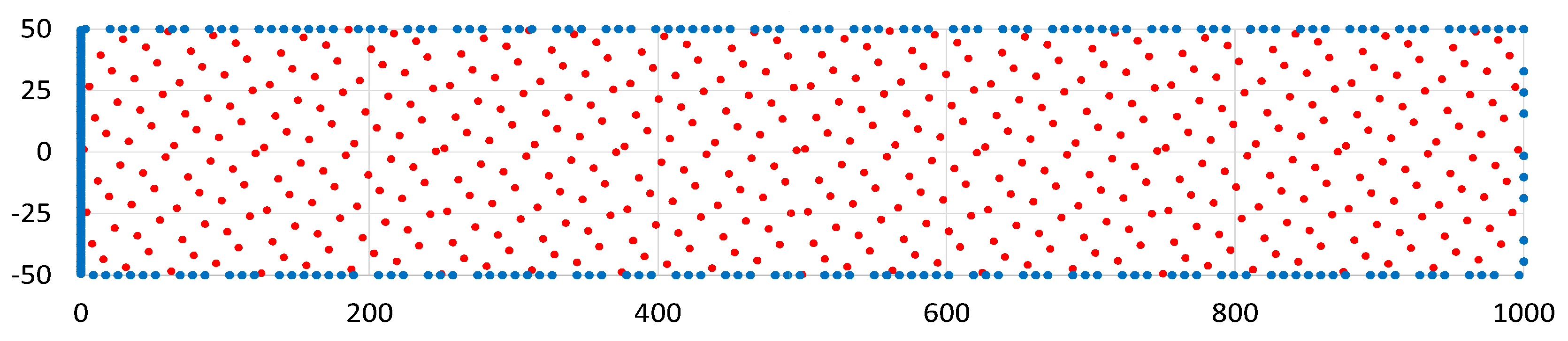
Figure 7.
The number of collocation’s points. 2D case. Grid 2.
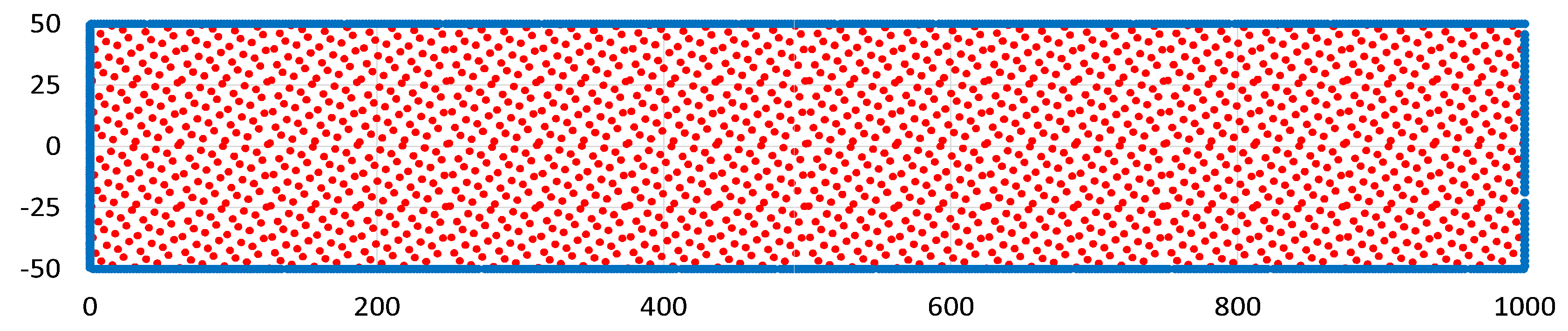
Figure 8.
Evaluation graph of a loss function. The number of iterations is plotted on the horizontal axis. 2D case.
Figure 8.
Evaluation graph of a loss function. The number of iterations is plotted on the horizontal axis. 2D case.
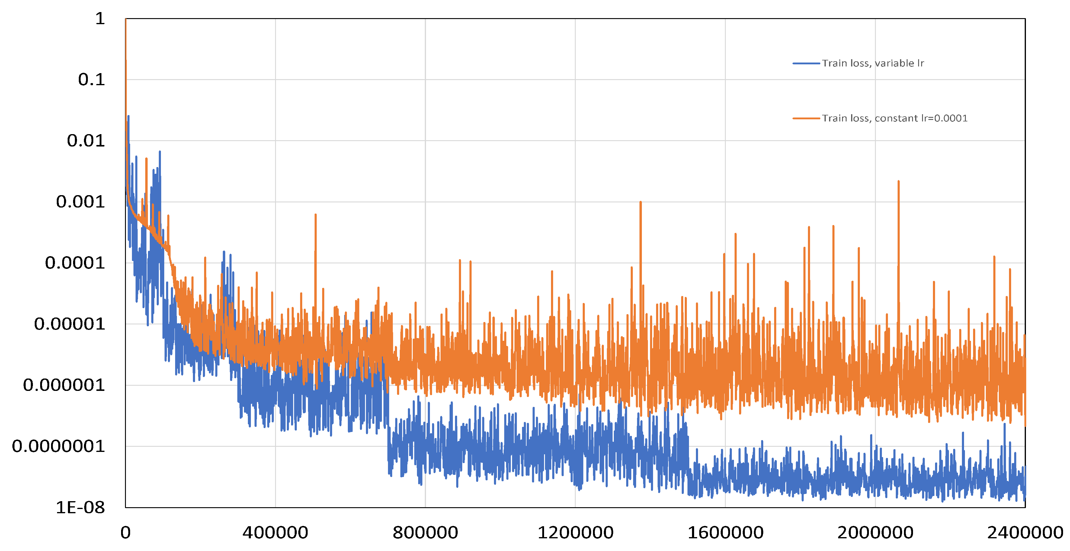
Figure 9.
The water level, calculated using Delft3D code (upper figure), calculated using PINN and constant learning rate lr=0.0001 (middle figure) and calculated using PINN and variable learning rate (lower figure). 2D forward case.
Figure 9.
The water level, calculated using Delft3D code (upper figure), calculated using PINN and constant learning rate lr=0.0001 (middle figure) and calculated using PINN and variable learning rate (lower figure). 2D forward case.
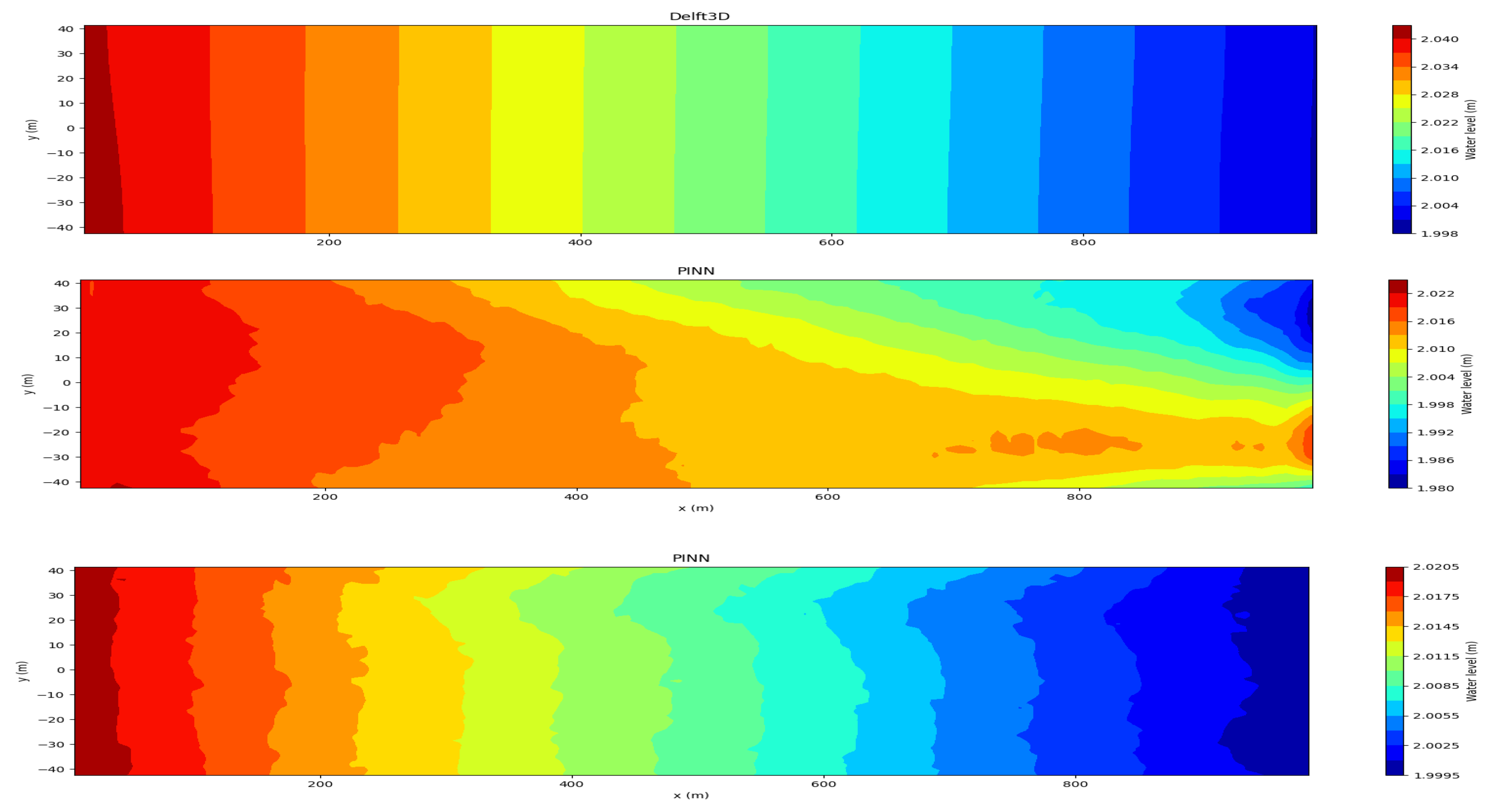
Figure 10.
Evaluation graph of a loss function. The number of iterations is plotted on the horizontal axis. 2D inverse problem. The first variant.
Figure 10.
Evaluation graph of a loss function. The number of iterations is plotted on the horizontal axis. 2D inverse problem. The first variant.
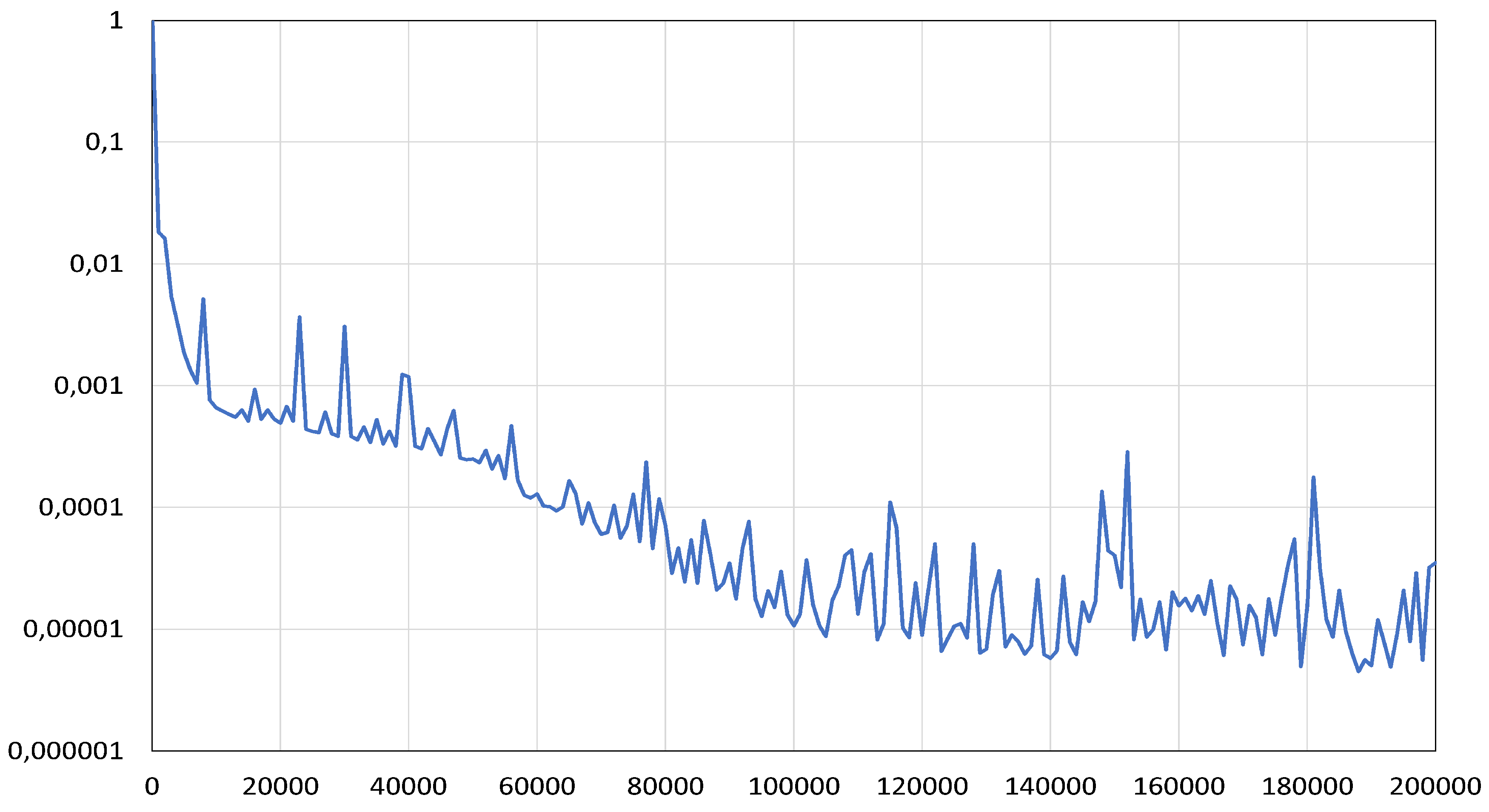
Figure 11.
The roughness coefficient. The orange curve is the exact value of the coefficient. The number of iterations is plotted on the horizontal axis. 2D inverse problem. The first variant.
Figure 11.
The roughness coefficient. The orange curve is the exact value of the coefficient. The number of iterations is plotted on the horizontal axis. 2D inverse problem. The first variant.
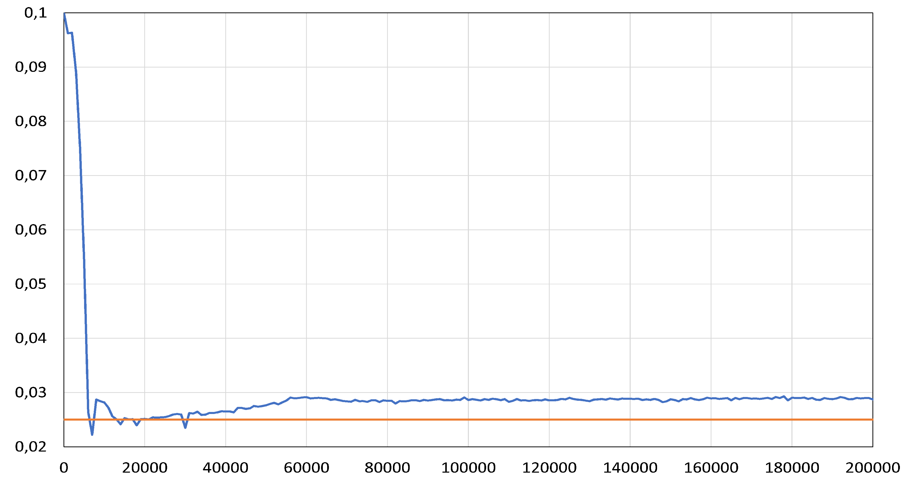
Figure 12.
x component of averaged velocity. 2D inverse problem. The first variant.
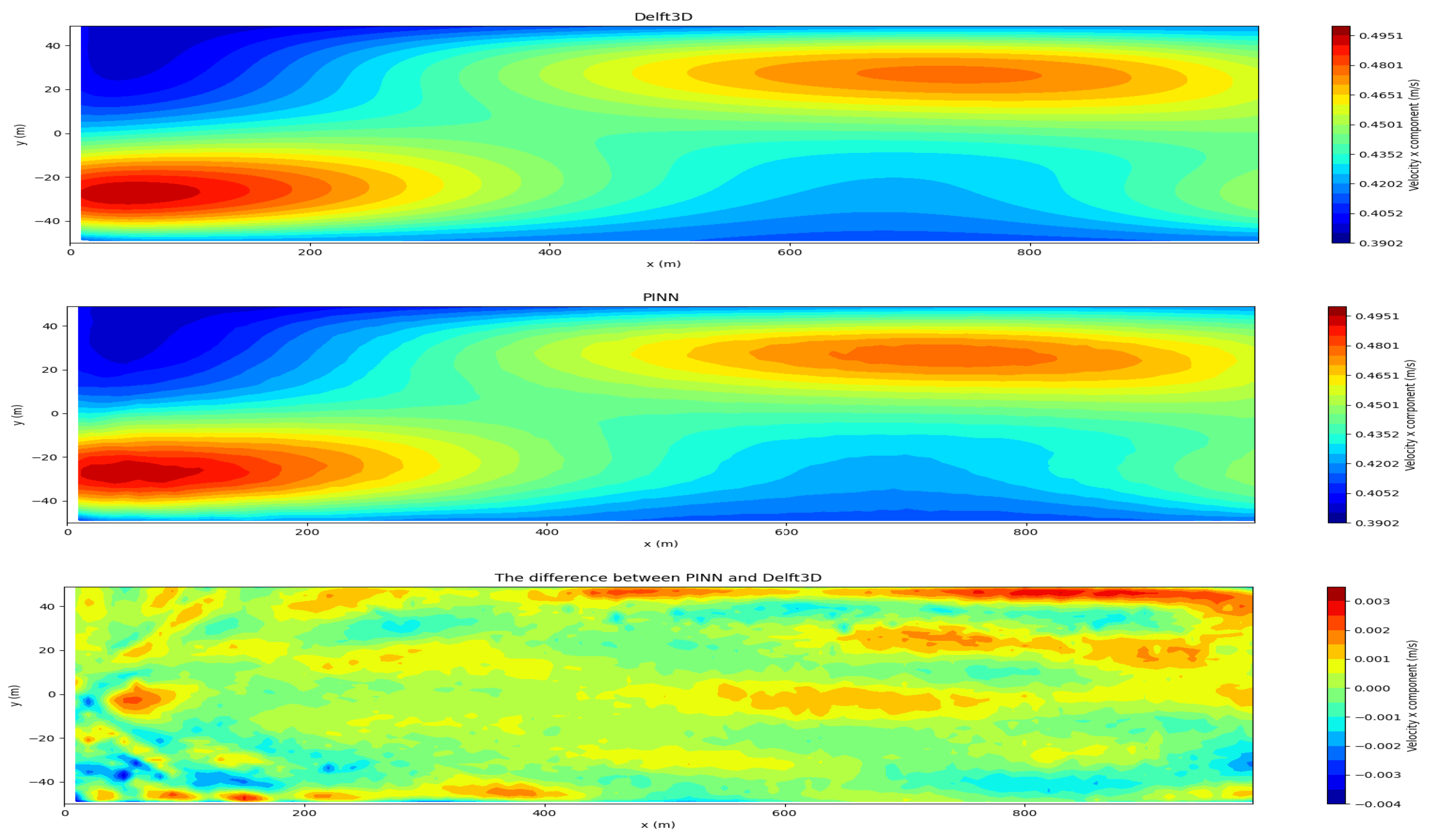
Figure 13.
y component of averaged velocity. 2D inverse problem. The first variant.
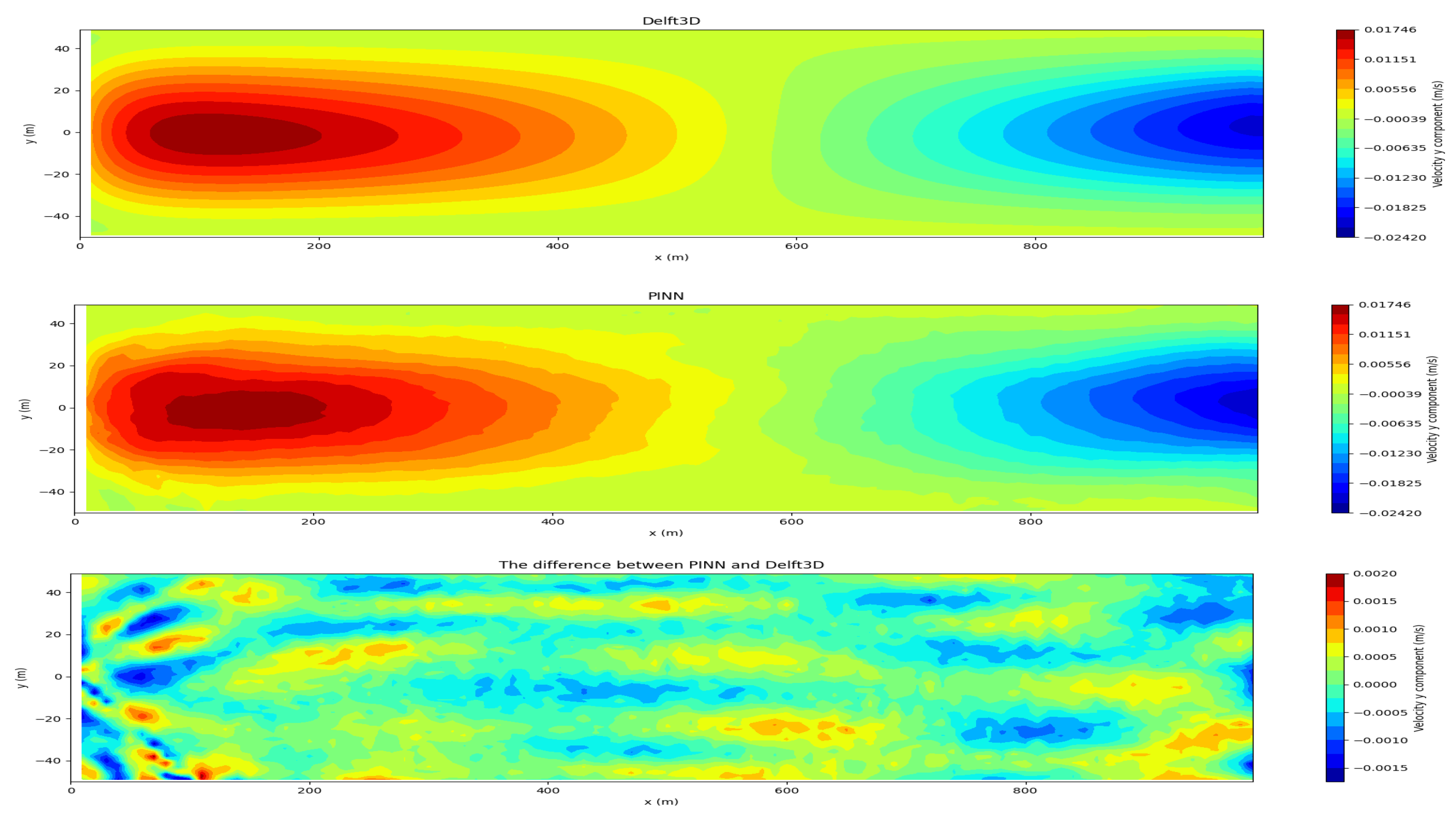
Figure 14.
Evaluation graph of a loss function. The number of iterations is plotted on the horizontal axis. The second variant of inverse problem.
Figure 14.
Evaluation graph of a loss function. The number of iterations is plotted on the horizontal axis. The second variant of inverse problem.
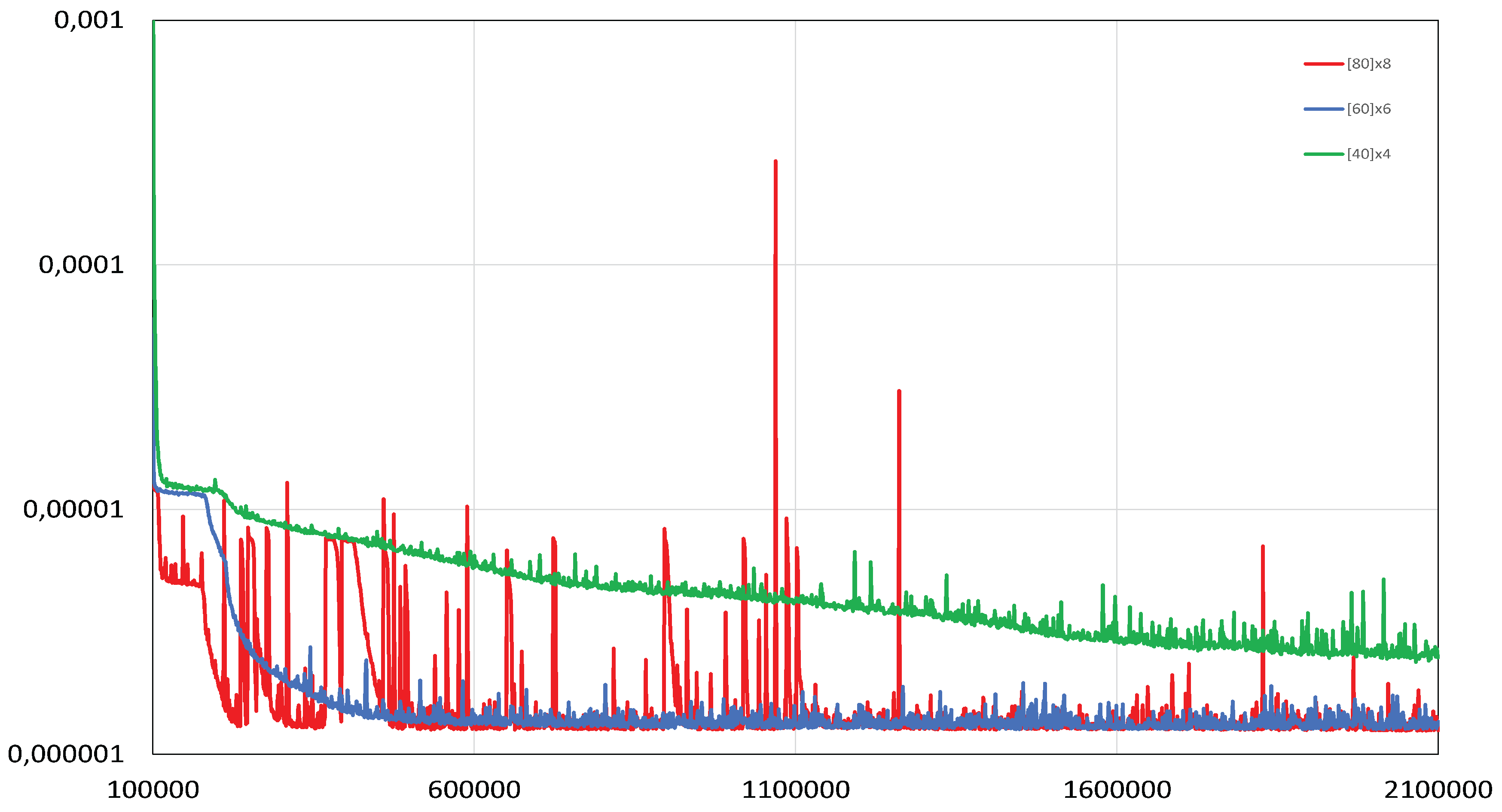
Figure 15.
The roughness coefficient. The orange curve is the exact value of the coefficient. The number of iterations is plotted on the horizontal axis. The second variant of inverse problem.
Figure 15.
The roughness coefficient. The orange curve is the exact value of the coefficient. The number of iterations is plotted on the horizontal axis. The second variant of inverse problem.
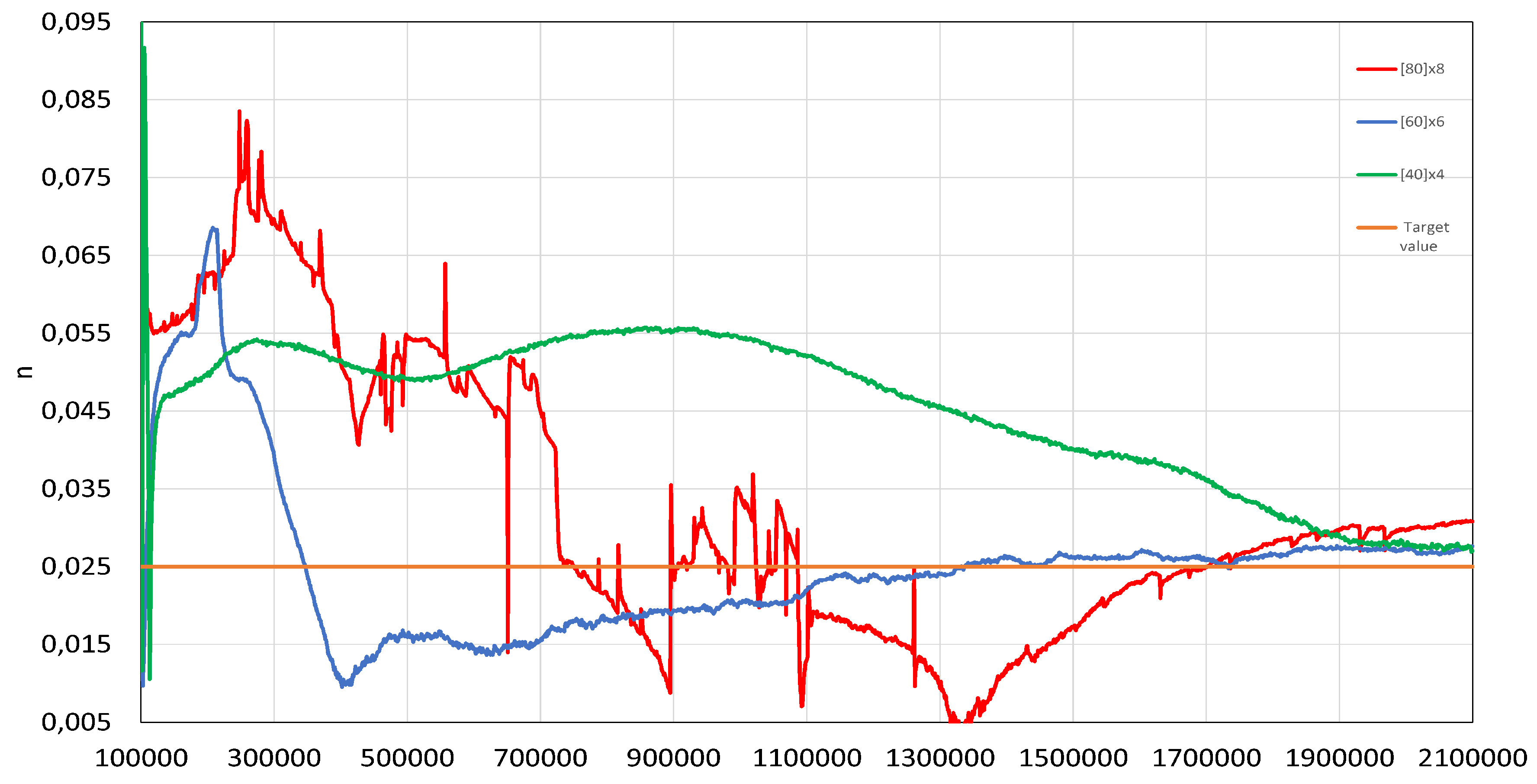
Figure 16.
Graphs of different values of loss function components for 2D inverse problem.
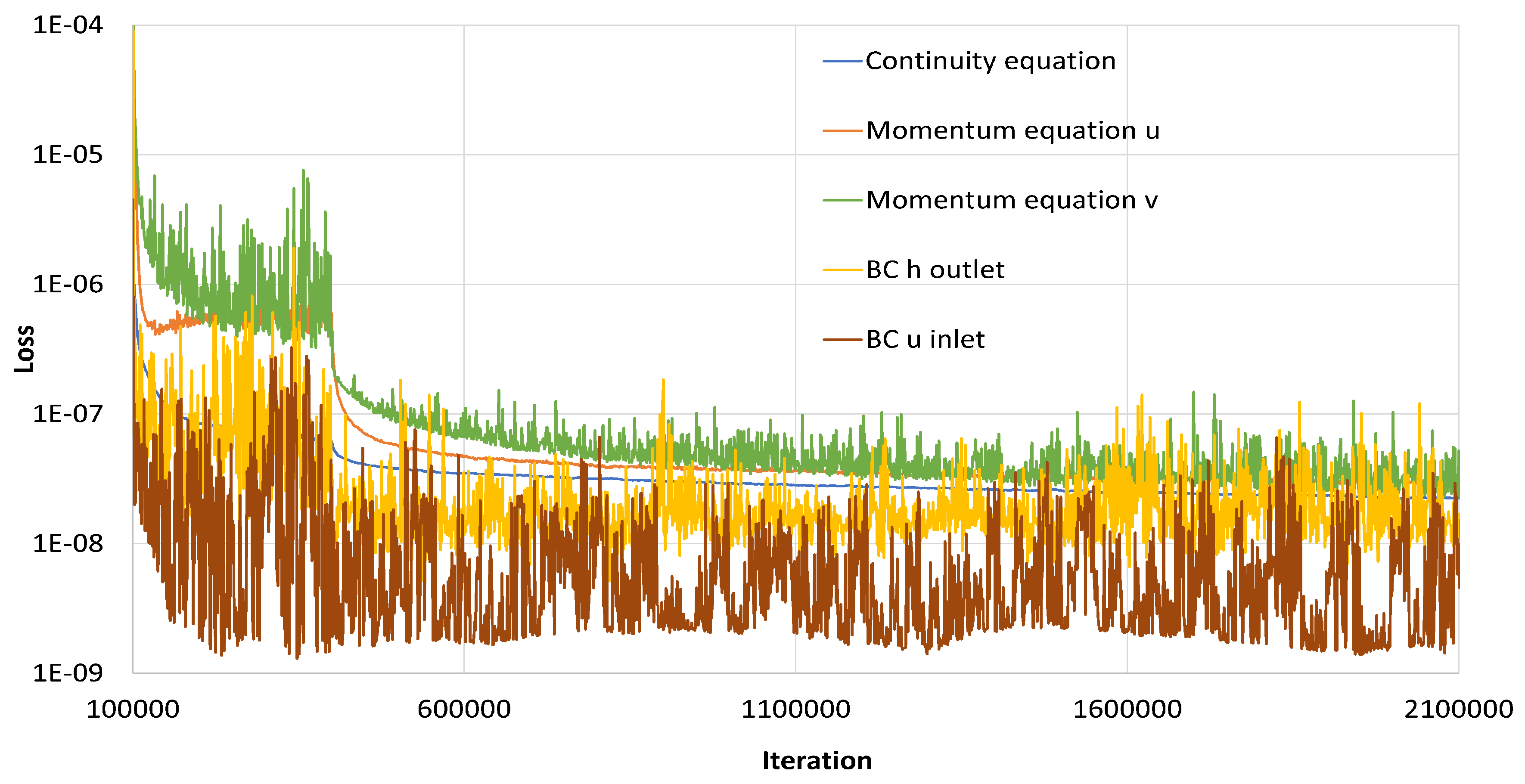

Table 1.
Roughness coefficient. Source from https://www.engineeringtoolbox.com/mannings-roughness-d_799.html (accessed on 27 June 2025)
Table 1.
Roughness coefficient. Source from https://www.engineeringtoolbox.com/mannings-roughness-d_799.html (accessed on 27 June 2025)
| Number | Value | Description |
|---|---|---|
| 1 | 0.022 | Earth channel - clean |
| 2 | 0.025 | Earth channel - gravelly |
| 3 | 0.030 | Earth channel - weedy |
| 4 | 0.035 | Earth channel - stony, cobbles |
| 5 | 0.035 | Floodplains - pasture, farmland |
| 6 | 0.050 | Floodplains - light brush |
| 7 | 0.075 | Floodplains - heavy brush |
| 8 | 0.15 | Floodplains - trees 1 |
Table 2.
The main hyperparameters
| Number of layers | Number of neurons | Name of test |
|---|---|---|
| 4 | 40 | test 1 - model 1 |
| 6 | 60 | test 2 - model 2 |
| 8 | 80 | test 3 - model 3 |
Table 3.
The main approaches and parameters
| Equations | Problem | Reference solution, Anchors |
|---|---|---|
| 1D | forward | Analytical |
| 1D | inverse | Analytical, Random points |
| 2D | forward | Delft3D |
| 2D variant 1 | inverse | Delft3D, Delft3D mesh |
| 2D variant 2 | inverse | Delft3D, Inlet |
Table 4.
The number of points for grid
| Grid | Points inner area | Points for borders |
|---|---|---|
| 1 | 500 | 200 |
| 2 | 2000 | 1000 |
Table 5.
Selection of value for Learning rate.
| Iterations | Learning rate |
|---|---|
| 0-100000 | 0.001 |
| 100000-300000 | 0.0003 |
| 300000-700000 | 0.0001 |
| 700000-1500000 | 0.00003 |
| 1500000-2500000 | 0.00001 |
Table 6.
Selection of points and Learning time
| Points | Learning time, hours |
|---|---|
| 500 | 1 |
| 2000 | 1 |
| 5000 | 1.3 |
| 20000 | 3 |
| 50000 | 6 |
Disclaimer/Publisher’s Note: The statements, opinions and data contained in all publications are solely those of the individual author(s) and contributor(s) and not of MDPI and/or the editor(s). MDPI and/or the editor(s) disclaim responsibility for any injury to people or property resulting from any ideas, methods, instructions or products referred to in the content. |
© 2025 by the authors. Licensee MDPI, Basel, Switzerland. This article is an open access article distributed under the terms and conditions of the Creative Commons Attribution (CC BY) license (https://creativecommons.org/licenses/by/4.0/).
Copyright: This open access article is published under a Creative Commons CC BY 4.0 license, which permit the free download, distribution, and reuse, provided that the author and preprint are cited in any reuse.


