Submitted:
12 July 2025
Posted:
15 July 2025
You are already at the latest version
Abstract
Agriculture plays a crucial part in the economy of many countries, particularly in de-veloping nations, where farming serves as the primary source of income for many in-dividuals. This study aims to enhance agricultural productivity through three key areas: yield prediction, price forecasting, and crop recommendation. The study utilizes remote sensing data and five distinct datasets to analyze agribusiness predictions. Following that, assess the performance robustness using new datasets, statistical analysis, and model parameters, and compare the results with earlier studies. The research fol-lows three main approaches: (1) Hybrid Technique for Yield Prediction: This method employs the Gradient Boosting Regressor, Cat Boost Regressor, and Bagging Regressor, utilizing the ensemble aggregation technique of stacking to predict crop yield. (2) Combined multinomial logistic regression and Yeo-Johnson transformer for Crop Recommendation: A logistic transformer is utilized to recommend appropriate crop varieties based on remote sensing data, aiming to improve precision agriculture. (3) Deep Neural Network for Price Forecasting: The study applies deep neural network models, especially a Multi-Layer Perceptron (MLP), to predict future crop market prices. Using MLP in price forecasting is a novel application in this context. Moreover, the food price data is evaluated using traditional algorithms, such as the Prophet and Auto-regressive Integrated Moving Average (ARIMA), to further validate the prices. Lastly, the study compares these approaches with previous research and conventional models to evaluate their effectiveness. Following that, LIME outlines model results alongside transparency, insight, and trust. Then, real-time deployment allows for immediate predictions. Last but not least, agribusiness integration corresponds to performance, business impact, and workflow. The ultimate goal of this forecast analysis is to meet the growing demand in the agricultural sector by providing farmers with tools for complete crop prediction. In the future, we intend to create a mobile application that will give users access to a multitude of data, making it simpler to forecast various crops for the agricultural market at every moment.
Keywords:
crop recommendation
; yield prediction
; price forecasting
; logistic transformer
; hybrid algorithm
; multi-layer perceptron
; deep learning-based approaches
; Prophet
; ARIMA
; conventional machine learning methods
; LIME
; integration of agribusiness systems
1. Introduction
Agriculture plays a crucial role in contributing to national finance, particularly in rural areas where agribusiness is a primary source of livelihood. With advanced technology such as Artificial Intelligence (AI), farming practices have significantly improved, offering greater comfort to growers and farmers. This article delves into previous studies on crop recommendations, yield prediction, price forecasting, and crop forecasting using remote sensing.
The research on crop yield prediction utilizes extensive databases to help farmers maximize yields, though current systems are offline and limited to a single server [1]. A key advantage is its ability to predict crops across multiple seasons. The study evaluates eight models to forecast yields based on soil and environmental conditions while integrating price forecasting to optimize profits [13]. Using Artificial Neural Networks (ANN), the model predicts yields for crops like sugarcane, rice, wheat, and cotton, considering soil, climate, and genotype interactions. Future improvements aim to incorporate both structured and unstructured data for enhanced accuracy.
Farming in rural India plays a vital role in the country's economy [4]. Studies comparing machine learning, statistical methods, and time series analysis for crop price prediction show that integrated models yield the lowest Root Mean Square Error (RMSE) values. Recent research highlights ongoing challenges in price forecasting and explores intelligent approaches and combination models [11, 12]. Findings suggest that decision trees provide the most accurate predictions when integrated with other models.
Although excessive fertilizer use is meant to increase crop output, it has negative environmental consequences. It damages ecosystems and contributes to financial losses for farmers and the environment. Recent studies emphasize the need for better chemical fertilizer management techniques to ensure sustainable crop production [10]. Another study [18] provides a wide-ranging literature review on using remote sensing data to enhance crop yield and quality. The review leverages unique text-mining approaches, but the algorithms may introduce some inherent biases. This study lists the modeling approaches and types of input data that performed best in various experiments. No comparable review article on this subject existed at the time of the research, underscoring the study's significance.
This article is structured into six sections: Figure 1. The introduction is in Section 1. Section 2 presents the findings of previous research. Section 3 details the methodology of the proposed system. Section 4 explains the experimental results, while Section 5 discusses the findings. Finally, Section 6 outlines recommendations and conclusions. Our research focuses on comprehensive crop-type suggestions, product estimates, and pricing predictions. By providing insights into yield growth, crop recommendations, and price forecasting, this study aims to enhance the agricultural system.
2. Literature Review
Predictive research on agricultural yield. In addition to Artificial Neural Networks (ANN), the study explores machine learning and deep learning techniques to improve prediction accuracy [14]. In agriculture-dependent countries like India, weather, climate, and economic conditions make crop prediction complex. However, estimation tools assist farmers in planning storage and marketing strategies. Data mining techniques, including the random forest algorithm, are increasingly used to analyze large datasets and generate forecasts. Recent studies highlight data mining as a promising approach for enhancing future crop yield predictions [15].
Compilation of earlier research on agricultural price forecasting. Research on agricultural price forecasting emphasizes its importance in reducing farmer losses and mitigating risks [2]. Studies utilize crop datasets and random forest-supervised algorithms for accurate price predictions, though further research is needed to estimate planting costs, especially with climate change impacts [3]. Techniques like decision tree regression and random forest regressors help forecast prices and recommend optimal sowing times. The goal is to provide reliable price forecasts to support farmer decision-making. Given the labor-intensive nature of farming, accurate predictions can enhance profitability and efficiency.
Strategies for predicting crop yields. This research introduces a mobile-compatible system that enables farmers to access yield predictions easily. Using GPS technology, it gathers data on location, soil type, and input for machine learning algorithms to estimate crop yields and optimize fertilizer application. Emerging agricultural trends highlight the impact of soil, climate, and market conditions on productivity. The system recommends the best crops to maximize yields and profits while minimizing losses. With global grain demand projected to rise by 2030, requiring a 2% annual yield increase to 580 Mt, improved soil management and farming practices will be essential in meeting this target [5].
Climate change and crop productivity. Research highlights the impact of climate change on crop productivity, with rising temperatures and shifting rainfall patterns leading to lower harvest values and affecting trade. These changes influence agriculture in both developed and developing countries, with regional climates determining the extent of the effects [6]. Higher temperatures generally reduce yields, while increased rainfall boosts them. Climate stress heightens the risk of yield loss, especially for weather-sensitive crops [7]. Strategies to enhance resilience include stress proteins and antioxidant defense systems [8]. Additionally, nitrogen plays a crucial role in boosting yields, with studies showing that higher nitrogen concentrations increase productivity in certain crops like Sushi hybrid maize, though sustainable management is necessary [9].
This study also investigates fertilizer management strategies and their role in improving crop productivity, particularly in Russian agriculture. By considering weather and soil conditions, the system provides optimized production rates and forecasts crop prices using the Minimum Support Price (MSP). Farmers can use these predictions to plant crops more effectively, forecast their income, and turn a profit.
Advances in the use of remote sensing to predict crop productivity. Remote sensing has become a valuable tool in agriculture, particularly for predicting crop productivity. A notable study [16] used data collected over 11 years from four crops: corn, soybeans, spring wheat, and winter wheat across 48 U.S. states. This study demonstrated the effectiveness of improved-resolution satellite imagery in forecasting crop yields. The findings show that as the resolution of satellite NDVI (Normalized Difference Vegetation Index) increases, the accuracy of crop yield regression models (R²) improves, highlighting the significant benefits of high-resolution data in agricultural applications.
Despite its comprehensive nature, the study did not account for regional variations in farming practices or technological adoption across the 48 states, which could potentially influence the results. It is important to consider this limitation when interpreting the findings.
Integration of remote sensing techniques in agricultural monitoring. Further research [17] discusses using various remote sensing techniques, including UAV (Unmanned Aerial Vehicle)-based imaging and satellite data, to assess plant health and growth stages. Integrating different data sources, such as visible and near-infrared light indices, is emphasized for effective biomass monitoring. These indicators are crucial for efficiently monitoring plant growth stages, making them essential tools for crop management and yield prediction.
Climate conditions' effects on crop productivity. A review [19] explores how climatic factors influence crop productivity and growth phases. It presents various types of satellite data, including Sentinel, MODIS (Moderate Resolution Imaging Spectroradiometer), Landsat, and Spot, and highlights the wide range of remote sensing data available for agricultural monitoring. The study shows that indices like Land Surface Temperature (LST) and NDVI are invaluable for crop management and environmental monitoring, demonstrating their effectiveness in improving agricultural practices and overall environmental management.
The role of weather forecasting in agricultural management. The research emphasizes the importance of accurate weather forecasting for agriculture, transportation, and disaster relief [20]. While predicting hyperlocal weather remains challenging due to complex atmospheric interactions, using Internet of Things (IoT) sensor networks can improve data collection and forecasting accuracy. The study calls for further research, particularly in air pressure estimation, though some areas may still be underexplored. In conclusion, remote sensing is vital for advancing agricultural practices like crop yield prediction, price forecasting, and crop recommendations. Continued integration of remote sensing technologies and refining forecasting methods can enhance crop productivity and food security, although challenges in regional variations, data collection, and predictive model accuracy remain.
2.1. Aim and Objectives
- Crop yield prediction using a hybrid meta-classifier
A hybrid meta-classifier enhances prediction accuracy and generalization by combining three models. Crop production is dependent on several variables, some of which may not be linearly related, including soil type, weather, temperature, nutrients, nitrogen, and crops. The purpose is to provide predictions that are more reliable and predictable so that estimation and allocation of resources are improved.
- Crop recommendation using combined Yeo-Johnson transformer and multinomial logistic regression
Transformers capture complex interactions and connections in the data. The logistic component enables multiclass crop suitability decision-making. The objective is to recommend the best crops to grow based on seasonal and geographic data (soil, rainfall, yield, area, fertilizer, pesticides, season, state).
- Price forecasting using MLP, RNN, CNN, ARIMA, and Prophet
Objective: To provide precise forecasts of future crop prices so farmers can act quickly and profitably in the market. MLP, RNN, CNN, ARIMA, and Prophet models have advantages.
3. Materials and Methods
The prediction process begins with the collection of crop data. Once the dataset is prepared, the model is trained, and the proposed prediction models are applied to evaluate the results. A hybrid meta-classifier is used for yield prediction, while a Logistic Transformer model is implemented for crop recommendations. For price forecasting, various models, including Multi-Layer Perceptron (MLP), Recurrent Neural Networks (RNN), Convolutional Neural Networks (CNN), the ARIMA model, and the Prophet model, are utilized.
Figure 2 visually represents each step in the predictive analysis process, including crop suggestions, yield prediction, and price forecasting. A process diagram is also included to illustrate the entire methodology of the current investigation. It illustrates the general procedures for prediction analysis. The following procedures are used for prediction analysis:
- Data preprocessing,
- Model training,
- Evaluation of models,
- Explainable AI (XAI) techniques such as LIME,
- Integration into an agribusiness system
- Experimental results and analysis
3.1. Data Gathering
One of the challenges in prediction analysis is the collection of diverse, huge datasets. There are six different data sources used in this study. The price forecasting dataset gathers and combines information from several sources, such as the markets, categories, and prices. There are 47,223 entries in it. Area, Year, Item, Months, Element, Code, Value, and Note are all present in the FAOSTAT_data_en_5-27-2025 dataset. FAOSTAT_data_en_5-27-2025 includes 171 rows. The huge remote sensing data set includes 325,834 data points and 175 attributes for crop recommendation. The yield prediction dataset consists of the following variables: Area, Item, Year, average_rain_fall_mm_per_year, pesticides_tonnes, avg_temp, and hg/ha_yield. In the yield dataset, there are 19,689 entries. The German yield has another yield prediction with 259,815 rows. There are six datasets used, as shown in Table 1.
3.1.1. Price Forecasting Dataset
This dataset contains food price data for Myanmar, sourced from the World Food Programme Price Database (https://data.humdata.org/dataset/wfp-food-prices-for-myanmar). The World Food Program Price Database covers foods such as maize, rice, beans, fish, and sugar for 98 countries and some 3000 markets. It is updated weekly but contains, to a large extent, monthly data. The data goes back as far as 1992 for a few countries, although many countries started reporting from 2003 or thereafter. The attributes consist of the date, location, region, state, market, area, category, commodity, unit, currency, price (Myanmar Kyat), and price (USD). Table 2 displays the price forecasting dataset samples. The date is from 2008 to 2024.
- Categories include various kinds of sources such as cereals and tubers, meat, fish and eggs, miscellaneous food, vegetables and fruits, oil, fat, pulses, and nuts.
- 12 states with diverse locations are Chin, Kachin, Kayah, Kayin, Magway, Mandalay, Mon, Rakhine, Sagaing, Shan, Tanintharyi, and Yangon.
- The many types of commodities comprise chickpeas, garlic, maize, oil, onions, potatoes, rice, salt, soybeans, tomatoes, and pulses.
- The economies of market places are Ah Nauk Pyin, Ah Nauk Ywe, Ahpauk Wa, Ai Cheng, Alel Than Kyaw, AnnMyo Thit, Aung San, Aung Zaya, Ba Yint Naung, Ban Wai, Barsara, Baw Du Pha, Bhamo, Bhamo Market 2, Bi Kin, Bilin Myo Ma Market, Bokyin, BoneSin, Butar, Buthidaung, Cherrygone, Chipwi, Chying Thung, Dein Aw, Demoso Myoma, Du Kahtawng, Falam, Galeng, Gangaw, Garayang, Gwa Myoma, Hakha Myoma Market, Hlaing Bwe Myo Ma Market, Hnaring, Ho Li, Home Shop.
- The commodity's price is stated in both USD and Myanmar currency.
In addition to the above World Food Program Price dataset, the price investigation results using an additional FAOSTAT dataset demonstrate that it is regionally boundless. The Food and Agriculture Organization of the United Nations (FAO) supports FAOSTAT, a free and open-access dataset used for trend forecasting, academic research, policy planning, data analysis, and model building.
Every FAOSTAT dataset (FAO, 2025. FAOSTAT information. United Nations Food and Agriculture Organization. From https://www.fao.org/faostat/en/, retrieved) is publicly available. FAOSTAT is a worldwide database maintained by the United Nations Food and Agriculture Organization (FAO). Crop production, trade, prices, land usage, employment, and other statistics related to agriculture are all included in the dataset. Area, Year, Item, Months, Element, Code, Value, and Note are all present in the FAOSTAT_data_en_5-27-2025 dataset. Table 3 demonstrates the price dataset for the FAOSTAT_data_en_5-27-2025.
3.1.2. Remote Sensing Dataset for Crop Recommendation
The "Crop mapping using fused optical-radar dataset" dataset is the donation of the University of California, Irvine (UCI) Machine Learning Repository (https://archive.ics.uci.edu/datasets).
On July 5th and July 14th, 2012, Unmanned Aerial Vehicle Synthetic Aperture Radars (UAVSAR) collected polarimetric radar data over an agricultural region near Winnipeg, Canada, and RapidEye satellites collected optical images. This data was combined and tabulated to create fused, bi-temporal optical-radar data for cropland classification. There are numerous varieties of maize, peas, canola, soy, oats, wheat, and broadleaf cultivation in this region. The sample data from remote sensing is displayed in Table 4.
3.1.2. Yield Prediction Dataset
On the websites of the FAO (https://www.fao.org/statistics/en) and World Data Bank (https://data.worldbank.org), the dataset is utilized. 28242 elements total, ranging from index 0 to 28241, make up the dataset. The dataset contains seven columns. The data types of most of the columns are float and integer. Area and Item are object data types. As there are 28242 non-null items in each column, it shows that the dataset contains no missing values. Table 5 presents a sample of the crop yield dataset attributes. Area, Item, Year, average_rain_fall_mm_per_year, pesticides_tonnes, avg_temp, and hg/ha_yield are the variables included in the crop yield dataset of Table 6. Table 7 shows the crop yield dataset sample.
The results show that it is the regional limit when utilizing additional German yield datasets in addition to the FAO yield dataset mentioned above. OpenAgrar makes the German yield (Duden, C., Nacke, C., & Offermann, F., 2024). German yield and area data for 11 crops from 1979 to 2021 at a harmonized spatial resolution of 397 districts. Scientific Data, 11(1), 95. https://doi.org/10.1038/s41597-024-02951-8) and area data for 11 crops are publicly available and free of charge. The study's agricultural yield dataset came from Duden, Nacke, and Offermann (2024). The dataset is obtained from the OpenAgrar source. We present an area and crop yield dataset for Germany from 1979 to 2021 in this publication. There are 214,820 yield and area data points in the dataset. Spring barley, winter barley, grain maize, silage maize, oats, potatoes, winter rape, rye, sugarbeet, triticale, and winter wheat are among the crops. The data are geographically resolved to 397 districts, each of which has an average area of 900 km². Table 8 displays the yield dataset for Germany.
3.2. Data Preprocessing
In machine learning, data cleaning and gathering are crucial steps, as they significantly impact the accuracy and performance of the model. The data preprocessing phase involves several activities, including data acquisition, importing necessary libraries, handling missing data, and encoding categorical variables.
Figure 3 illustrates the data preprocessing stage, which transforms an unclean dataset into a clean, usable one. Raw data from multiple sources is first collected, and any missing or null values are addressed to create a readable format. The proposed models mustn't be trained until these missing values are appropriately handled.
The datasets for yield prediction, crop recommendation, and price prediction are sourced from public websites.
3.3. Data Visualization
The dataset includes a wide range of numerical features from remote sensing data
derived from two main sources: radar-based data and optical data collected by RapidEye satellites. Combining these two data types, the analysis has consistently yielded highly accurate crop identifications across various characteristics and developmental stages. Visualization techniques such as heat maps and box plots are used to better understand the data. These visualizations help in identifying patterns and distributions within the dataset. Additionally, a correlation analysis is performed, which evaluates 175 features from the remote sensing data.
Figure 4 illustrates the correlation analysis of the remote sensing data, providing further insights into the relationships between different features.
In Figure 5, the x-axis shows the crop dataset columns including Area. These inputs are represented on the x-axis of the subplots, while the hg/ha_yield of the target variables is displayed on the y-axis. Figure 6 shows the date, location, region, state, market, area, category, commodity, unit, currency, price (Myanmar Kyat), and price (USD). All the data entries are displayed. The markets, cities, regions, currency, domain categories, and years affect the goods. The date is from 2008 to 2024.
3.4. Train and Testing Split
The dataset includes columns with data types as strings, which cannot be directly interpreted as numerical values. To facilitate visualization and analysis, these categorical variables are changed into numerical values using One Hot Encoding. This technique transforms category variables into binary vectors. Next, the Robust Scaler is applied to standardize the train and test data. The dataset is then split, with 30% allocated for testing and the remaining 70% applied for training the model.
Once the data is partitioned and preprocessed, crop recommendations, yield predictions and price forecasting are performed using the proposed logistic transformer, hybrid algorithms, and deep learning strategies.
3.5. Using a Logistic Transformer to Recommend Crops with Remote Sensing Data
In regression analysis, logistic regression is employed to forecast future outcomes, especially when the dependent variable is categorical. Unlike linear regression, which predicts continuous variables, logistic regression is specifically designed to predict a categorical variable by evaluating the relationship between the dependent variable and one or more independent factors.
For logistic regression to be effective, a sufficiently large sample size is necessary to represent the different categories of the dependent variable. Without a large, representative sample, the model may lack the statistical power to identify significant effects. Figure 7 provides an overview of the logistic regression process.
Logistic regression is primarily used for binary classification, where the objective is to forecast the likelihood that an input falls into one of two categories. These classes are typically represented by the values 0 and 1.
The formulation in mathematics of logistic regression is as follows:
- Equation (1) gives a thorough explanation of the weighted summation of the input variables.
- Equation (2) estimates the probability that unseen data will belong to a specific class.
Multiple linear equations,
- Weighted addition of inputs
Sigmoid Function
- Assume the probability of unseen data belonging to the class
The lambda parameter is fitted using the designated method via the method, and this transformer performs the Box-Cox-transform elementwise. Box-Cox requires the input data to be positive. Not even zero is acceptable. But Yeo-Johnson accepts zeroes or negative values.
- In Equation (3), add 1 to the data (y), raise it to the power of λ, deduct 1, and divide by λ when λ = 0.
- In Equation (4), if λ ≠0: Take the log and add 1 to the data y.
- In Equation (5), if λ is not equal to 2, take 1 from the data and multiply the result by 2 - λ.
- In Equation (6), take the log of the data log, y minus 1, when λ = 2.
After separating the dataset into train and test sets, the Yeo-Johnson power transformation is applied to the data. This transformation strategy is utilized in conjunction with logistic regression to improve the model's performance. Data standardization is not required until the transformation is complete. The application of the Yeo-Johnson transformation has led to an increase in test accuracy.
Following that, crop recommendations are made using the Variance Inflation Factor (VIF). In statistics, the VIF quantifies the magnitude to which collinearity increases the variance of an estimated regression coefficient. Specifically, it measures the ratio of the variance of a parameter estimate when fitting a full model with other parameters to the estimate's variance when the parameter is fitted alone. A higher VIF indicates higher collinearity, which can lead to less reliable estimates of regression coefficients.
More importantly, the hyperparameter values of a Logistic Transformer model for crop recommendation are described in a well-organized Table 9.
3.6. A Hybrid Approach for Yield Prediction
A previous study utilized deep learning to perform precise computations for selecting the optimal crop when multiple choices were available. The proposed methodology predicts crop yield using a hybrid approach that combines three different regression models. This technique was tested on a crop dataset, considering key factors such as Rainfall, Fertilizer use, Temperature, Nitrogen, Phosphorus, Potassium, and Yield. The results demonstrated that the approach effectively improves yield prediction accuracy. Figure 8 illustrates the hybrid model architecture used for the Gradient Boosting Regressor + Cat Boost Regressor + Bagging Regressor.
Procedures for Execution
- Step 1: First, import the crop dataset with several 1000 entries.
- Step 2: Put the required libraries and packages.
- Step 3: The data has been preprocessed.
- Step 4: The data is split into trains and test sets to build up the dataset.
- Step 5: Following this, a model is built using hybrid algorithms (Cat Boost Regressor, Gradient Boosting Regressor) and machine learning (Bagging Regressor) techniques, forecasting the ideal yields that ought to be produced.
- Step 6: The testing set evaluates the meta-classifier's execution.
- Step 7: The hybrid returns the Accuracy, Mean Score, MSE, and R2_score.
The parameters of the hybrid yield prediction method are learning rate, n_estimators, and random_state. Hybrid algorithms use features, variables, and encoders. The learning rate (0.001) is used to train the model. We use K-fold cross-validation to assess the model for Fold 10. Performance is measured using accuracy, R2 score, Mean Score, and MSE.
3.7. Price Forecasting
Agriculture takes on a pivotal role in the economy, with the prices of agri-horticultural products significantly impacting both farmers and consumers. Accurate crop price forecasting is essential for minimizing economic risks and helping stakeholders make informed decisions. However, crop prices are influenced by various factors, including supply chain disruptions, market demand, weather conditions, and regulatory changes. Due to the complex and nonlinear nature of price fluctuations, traditional forecasting methods often fail to provide reliable predictions.
Figure 9 illustrates the proposed price forecasting procedure, designed to address these challenges. Existing systems often face difficulties in integrating and utilizing diverse data sources, such as market trends, soil quality, and weather conditions, resulting in unsatisfactory analysis. By overcoming the limitations of current systems, the proposed approach aims to offer a more accurate, adaptable, and effective solution for agricultural price forecasting.
Deep learning techniques have proven effective in price forecasting, with three primary types of neural networks commonly used. Compare these models' performance to that of other conventional algorithms that are frequently employed in agriculture, such as the Prophet model and ARIMA time series forecasting. The five models that are proposed are:
- MLP (Multi-Layer Perceptron)
- CNN (Convolutional Neural Networks)
- RNN (Recurrent Neural Networks)
- ARIMA model
- Prophet model
3.7.1. Multi-Layer Perceptron (MLP)
Machine learning (ML) and artificial intelligence (AI) offer powerful tools for price forecasting, particularly in the agricultural sector. Among these, Multi-Layer Perceptron (MLP) is highly effective in extracting deep features and modeling sequential data. Developing a reliable MLP model to forecast Agri-horticultural commodity prices, including vegetables and peas, can significantly benefit policymakers, traders, and farmers by enabling informed decision-making.
MLP is a sort of feedforward artificial neural network and represents one of the most fundamental deep learning architectures. An MLP model includes multiple fully connected layers, where each successive layer applies nonlinear functions to the weighted sum of outputs from the preceding layer. This design allows MLPs to process structured data with fixed dimensions and independent characteristics, uncovering intricate patterns and correlations within the dataset.
One of the critical factors influencing an MLP’s performance is the total number of trainable parameters, which is determined by the network's depth and layer configurations. The proposed MLP architecture consists of 7,703 trainable parameters, with a detailed breakdown provided in Table 10. By leveraging MLP’s ability to handle complex data relationships, this model aims to enhance the accuracy of agricultural price forecasts while addressing computational efficiency challenges in modern deep learning systems.
3.7.2. Convolutional Neural Networks (CNNs)
Convolutional Neural Networks (CNNs) symbolize another kind of deep neural network widely used in artificial intelligence (AI) systems. CNNs are designed to automatically extract features from large datasets, enabling efficient learning and task completion. The detailed structure of the proposed CNN model is outlined in Table 11.
Unlike Multi-Layer Perceptrons (MLPs), which rely on fully connected layers, CNN models utilize one or more convolutional layers to extract relevant features from input data. These layers apply convolution operations, where each layer consists of nonlinear functions of weighted sums computed across spatially adjacent subsets of the input. The weights in each layer are derived from the preceding layer, allowing the model to recognize complex patterns and spatial hierarchies.
A typical CNN architecture includes several key components:
- Convolutional layers for feature extraction
- Pooling layers to decrease dimensionality and retain essential information
- Fully connected layers to interpret extracted features
- Additional layers to enhance model performance
3.7.3. Recurrent Neural Networks (RNNs)
Recurrent Neural Networks (RNNs) are specifically designed for processing sequential data and are widely used in time-series forecasting. Contrary to conventional neural networks, which treat each input independently, RNNs incorporate both previous samples and the current input, allowing them to capture temporal dependencies. The connections between nodes form a directed graph along the time sequence, enabling the network to learn from past information.
A key feature of RNNs is their internal memory, which stores computation data from earlier samples. This permits the network to retain contextual information and improve predictions with time. Each subsequent layer in an RNN consists of multiple nonlinear functions of weighted sums derived from both the current input and the previous state.
The fundamental building block of an RNN is a "cell", which processes sequential data. These cells are organized into layers, enabling the network to learn patterns and dependencies effectively. The proposed RNN model consists of 50 units, designed to recognize patterns in sequential data. A fully connected Dense layer follows this recurrent layer to refine the final predictions. The compiled RNN model architecture is detailed in Table 12.
3.7.4. ARIMA Model
An effective statistical technique for time series forecasting is the ARIMA model, which stands for Auto Regressive Integrated Moving Average. When predicting non-seasonal time series data, the ARIMA algorithm is quite effective. The crucial phases are fixing the model's parameters, fitting the data, confirming the outcomes, and making the data stationary. The following Table 13 of pseudocode provides the primary steps for using the ARIMA algorithm for time series forecasting:
3.7.5. Prophet Model
- Compared to ARIMA, Prophet is a more flexible and user-friendly model that automatically manages seasonality, changepoints, and missing data. It also offers distinct representations of the model's constituent parts.
- However, ARIMA is more outlier-sensitive and necessitates more manual model parameter adjustment. It might also be more challenging to interpret and necessitate a greater comprehension of the fundamental statistical ideas.
- However, it is more adaptable because ARIMA can be expanded to the SARIMAX model, which permits the inclusion of exogenous variables.
- The performance of the model is contingent upon the type of data and the task in question; it is vital to remember this.
- Time series forecasting problems are successfully solved using Prophet and ARIMA; nevertheless, it's crucial to test various models and approaches, assess each one's performance, and choose the best one for the dataset.
3.8. A Statistical Evaluation of Models
The performance of these models is evaluated using statistical analyses, including accuracy, F1 score, recall, Mean Squared Error (MSE), and mean score.
Mean Absolute Error (MAE) calculates the absolute value of the error that exists between the actual and anticipated values and then averages it. MAE represents the error's actual size because it takes the error's absolute value.
A statistical metric called R-squared quantifies how well the independent variables can account for variations in the target variable. The range is 0 to 1. When the R2 is 1, it indicates a perfect match; when it is 0, it indicates that the variance cannot be explained.
Root Mean Squared Error (RMSE) which is the root of the MSE, is utilized since the MSE value, which is the square of the error, tends to be bigger than the real error average. The greater the inaccuracy, the higher the weight is reflected because the error is squared.
MAPE (Mean Absolute Percentage Error) converts MAE to a percentage; has the same limitations as MAE; the model is biased.
3.9. Challenges
During this project, we encountered several problems, including:
- To achieve optimal outcomes, preprocessing and choosing an appropriate dataset enhance the project's appeal.
- Minimal processing power is required for training regression models.
- The gathering of various large datasets for prediction analysis presents a challenge.
4. Results
4.1. Recommendation of Crops
A total of 325,834 remote sensing data points are generated from the public dataset. The comparative testing for the crop dataset from the Indian Chamber of Food and Agriculture includes 2,200 entries of crop and key variables such as temperature, humidity, pH, rainfall, and NPK (nitrogen, phosphorus, and potassium) measurements, along with crop labels. The user inputs parameters like temperature, humidity, rainfall, and NPK levels into the crop recommendation system, which then uses the proposed Logistic Transformer to suggest suitable crops for planting.
The system's performance is evaluated by comparing the crop recommendation results using both crop data and remote sensing data. The crop dataset, which includes 2,200 rows for each crop type, such as kidney beans, rice, cotton, and maize, is separated into distinct crop groups, with varying outcomes based on the input data. For the crop data, the dataset is split into 71% testing and 77% training data.
When applying the Logistic Transformer to remote sensing data, it achieves an impressive 98% training accuracy and 0.98% testing accuracy. The accuracy of the Logistic Transformer significantly varies with different dataset sizes, with larger datasets proving to be a better fit for this model.
Table 15 compares the Logistic Transformer results using both crop data and remote sensing data, providing clear evidence of the system's accuracy. It also displays the testing and training performance results for different crop types, offering valuable insights for users seeking crop recommendations.
In conclusion, the Logistic Transformer with Remote Sensing Data is significantly more effective in both training and testing, likely due to the larger and more informative dataset. The crop data model could benefit from additional data or feature engineering to improve its accuracy. Table 13 provides a summary of the comparison's findings and emphasizes how effective the suggested model is for both kinds of data.
The proposed recommended logistic transformer algorithm's accuracy of 98% is compared with previous research [4]. In this paper, MLR gets 60%, SVM obtains 75%, ANN receives 86%, KNN has 90%, and Random Forest (RF) for the crop recommender system achieves 95% accuracy [4]. Table 16 indicates the accuracy comparison of the earlier studies.
4.1.1. Analysis of Crop Recommendation Results
The Logistic Transformer with Crop data shows significantly lower performance, with only 77.3% training accuracy and 71.35% testing accuracy. This suggests that while the model is capable of learning from the crop data, its capacity to generalize to new, invisible data is weaker compared to the remote sensing data model.
- Size of the Dataset: The model using remote sensing data has access to a much larger dataset (325,834 data points), likely contributing to its higher accuracy. The crop data model uses 2,200 entries.
- Data Quality and Features: Remote sensing data likely provides richer, more detailed information on environmental and crop conditions, whereas crop data may be more limited in scope or not as diverse, affecting model performance.
- Overfitting and Underfitting: The crop data model could be underfitting due to a smaller dataset, while the remote sensing model has enough data to capture patterns without overfitting.
4.2. Yield Prediction
A hybrid algorithm incorporating Area, Item, Year, average_rain_fall_mm_per_year, pesticides_tonnes, avg_temp, and hg/ha_yield is used to forecast crop yield per acre. Data range index of 28242 entries total included. Accurate yield prediction is crucial for farmers and agricultural stakeholders, as it directly impacts decision-making and risk management. Seasonal variations play a significant role in agricultural productivity, making reliable forecasting essential.
Previous research indicates that geographical areas ("Area") significantly influence crop yield ("Products"). Our study focuses on developing a meta-classifier that predicts yield outcomes based on key environmental and agricultural factors, as illustrated in Figure 10. Varieties of crops, rainfall average, temperature fluctuations, and pesticide tone availability are among the primary determinants of crop yield.
To enhance crop yield prediction, we implement a hybrid machine learning model that integrates Gradient Boosting Regression, Bagging Regression, and CatBoost Regression. The results of this metaclassifier are presented in Figure 11. The model forecasts yield based on area, item, temperature, rainfall, etc. In the figure, the blue line represents the predicted values, with the x-axis showing actual values and the y-axis displaying expected values. The training and testing accuracy of the Meta Classifier is displayed in Table 18.
The hybrid model achieves 98% accuracy, one of the most reliable outcomes in agricultural yield forecasting. The model’s performance is further validated using K-Fold cross-validation (cv=10). For the German yield datasets and the FAO yield datasets, Table 14 provides a detailed breakdown of the square error, accuracy, and R² score to demonstrate the effectiveness of the suggested strategy. In closing, the outcomes of the hybrid models are compared with those of the other models, including bagging regressor, XGboost, KNN, gradient boost, random forest, decision tree, and linear regression. The results are indicated in Table 17.

Table 17.
The results of the hybrid models' comparison with the other models.
| Model | Accuracy | Meaning Square Error | R2_score |
|---|---|---|---|
| Hybrid Model | 0.982941 | 123845573.323863 | 0.982941 |
| Comparison of results with the other seven models | |||
| Linear Regression | 0.028421 | 7201484234.197933 | 0.028421 |
| Random Forest | 0.157611 | 6243913909.361324 | 0.157611 |
| Gradient Boost | 0.143967 | 6345039142.634174 | 0.143967 |
| XGBoost | 0.042164 | 7099623711.649448 | 0.042164 |
| KNN | 0.353193 | 4794229490.966104 | 0.353193 |
| Decision Tree | -0.058247 | 7843881514.231441 | -0.058247 |
| Bagging Regressor | 0.158734 | 6235585480.723247 | 0.158734 |
Table 18.
The accuracy of the Meta Classifier's training and testing.
| The accuracy of the Meta Classifier Model Train is 99%. |
| The accuracy of the Meta Classifier Model Test is 98%. |
4.3. Price Forecasting
Agricultural price prediction plays a crucial role in market analysis and decision-making [13]. Our model forecasts market prices for various crops, helping farmers and traders maximize profitability by choosing the optimal selling season. Since crop prices can fluctuate significantly within a week, we recommend predicting agricultural product prices before entering the market to reduce financial uncertainty.
Our dataset consists of training and test data, with a focus on real-time data collection from the World Food Program Price Database. However, when the dataset is limited, prediction accuracy decreases. Throughout the study, we analyze price fluctuations over time by using daily updated pricing data. The model leverages actual applied daily datasets for accurate and dynamic price forecasting.
Deep learning has become an effective solution for machine learning problems, particularly in fields such as time-series forecasting and image recognition. In this study, we compare three neural network types: Multi-Layer Perceptron (MLP), Recurrent Neural Network (RNN), and Convolutional Neural Network (CNN) using a crop pricing dataset. RNN and CNN were used in many earlier studies. The experiments are conducted using Python and Keras.
In order to assess model performance, we use Mean Absolute Error (MAE) and Mean Squared Error (MSE) metrics. Different neural network topologies are tested to identify the most suitable model based on forecast accuracy and data characteristics.
The three models’ performance is illustrated in Figure 12, showing loss per epoch across 100 training partitions. The MLP model achieves lower loss values (0.019, 0.016, 0.440, and 0.139), demonstrating superior efficiency. Compared to RNN and CNN, MLP outperforms in sequential data tasks, providing enhanced accuracy and predictive capabilities. The term "loss per epoch" refers to the loss function value calculated after each training cycle, as shown in Figure 12.
Price predicting results from the FAOSTAT dataset include an R-squared of 0.874879715984535 and a Mean Absolute Error of 16.60228836460122.
To achieve highly accurate crop price predictions, we construct a dense neural network model. The MLP model correctly classifies data 98% of the time, making it the most accurate among the three architectures evaluated. Deep neural network-based price predictions are illustrated in Figure 12, where the Y-axis implies loss values, and the X-axis denotes epoch dates. Overall, the MLP model proves to be a new effective model for future agricultural price forecasting, outperforming CNN and RNN in accuracy and reliability.
Table 19 displays a comparison of the price forecasting skills of MLPs, CNNs, and RNNs by loss, MAE, MAPE, RMSE, and R-squared.
In this study, we compare CNN (Convolutional Neural Networks) and RNN (Recurrent Neural Networks), both of which are widely used in neural network architectures. These models, particularly useful for time-dependent price forecasting, share several key advantages: Time Dependencies, Generalization and Backpropagation. Time Dependencies: CNN and RNN models are specifically designed to predict prices based on temporal dependencies, capturing the intricate patterns in price fluctuations over time. Generalization: The models are effective at generalizing price predictions to previously untested situations, maintaining high accuracy even when applied to new data that wasn't part of the training set. Backpropagation: When combined with the backpropagation technique, CNN and RNN models demonstrate their ability to handle significant variations in price prediction accuracy, improving the reliability of their forecasts.
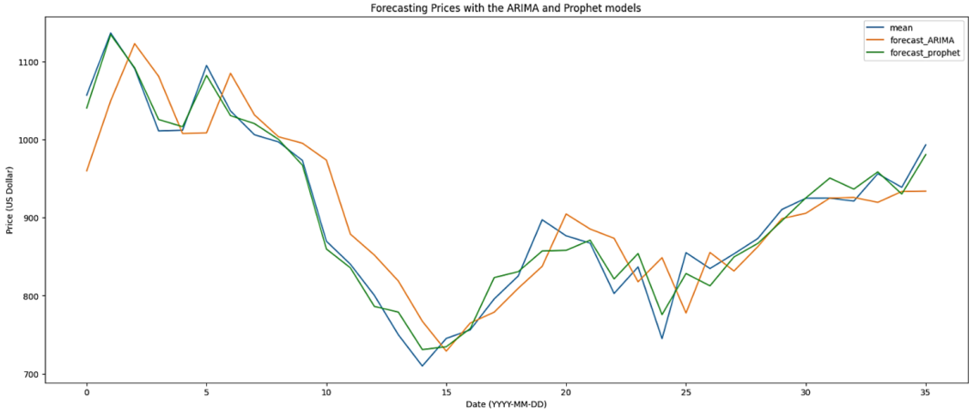
Figure 13 displays a comparison of price forecasts from the ARIMA and Prophet models. Plotting the actual data against the two suggested models that are expected is shown. A numerical dataset analysis is done in price forecasting. Blue lines show the associations between each pair of actual data. Figure 13 shows the green and orange lines, respectively, representing the ARIMA and Prophet predictions. For pricing forecasting, the RMSE of the ARIMA model is 997.97, which is significantly higher than that of the Prophet model. The Prophet model had the lowest RMSE value of 817.12.
To further validate the effectiveness of these models, testing was repeated using a real-world dataset consisting of Myanmar food prices, sourced from the World Food Program Price Database (https://data.humdata.org/dataset/wfp-food-prices-for-myanmar). This dataset contains 49,779 entries and represents the actual costs of food items in Myanmar. Five models are suggested. Testing the performance of these MLPs, CNNs, and RNNs with other traditional Prophet models and ARIMA time series forecasting methods. The testing process ensures the models' worldwide applicability and their capability to make accurate predictions in different contexts.
Figure 13.
Comparing pricing forecasts using the ARIMA and Prophet models.
4.4. LIME (Local Interpretable Model-agnostic Explanations)
Following price, yield, and crop recommendation prediction using suggested models, further application of Explainable AI (XAI) techniques enhances end users' ability to comprehend and assess forecasts. LIME of XAI makes for pricing, crop types, and yield analysis more interpretable globally.
Included in the LIME processes are:
- Gather agricultural data such as crop types, product prices, yield predictions, and classifications.
- Preprocess the data to clean and prepare it by filling in the missing values. Train models to generate predictive models.
- Instance Selection: Pick a particular prediction situation that needs to be explained.
- Feature variation: Change the feature values of the chosen instance to introduce variations and create a synthetic dataset.
- Model Prediction: Use the trained model to generate predictions for the modified cases to evaluate the impact of feature changes on the outcomes.
- Training Surrogate Models: Create a user-friendly surrogate model.
- Producing Explanations: Examine the surrogate model to identify and highlight the crucial factors impacting the prediction, which will assist users in understanding how the model makes.
Price forecasting, crop recommendation, and yield prediction results are displayed after setting the LIME for regression, defining the prediction function, and showing the test prediction. The crop recommendation LIME results are shown in Figure 14, while Figure 15 displays the yield prediction LIME results. Forecasts of prices are presented in Figure 16.
4.5. Integrated into an Agribusiness System
An integrated system that supports agribusiness decision-making by integrating three predictive components. The objective is to forecast prices, recommend the best crops, and predict crop yields using a single AI architecture. The integration into the design of an agricultural system API (Application Programming Interface) is depicted in Figure 17.
This technology improves strategic agribusiness planning by efficiently integrating machine learning models and many data sources into a unified architecture. This application integrates three predictive components to provide a unified AI-driven dashboard that aids in agriculture decision-making. Figure 18 displays the integration into an agricultural system's design.
The AI-driven dashboard depicted in the figure can forecast crop yields and prices, suggest appropriate crops, and export data to a PDF. In Fig. 18, the functions of Select Sample Indices and PDF Export serve the predictive system. This figure displays the AI-powered dashboard that forecasts crop yield, prices, appropriate crops, and exports results to a PDF. Figure 19 displays the dashboard information in PDF format.
5. Discussion
In this study, we examine the most efficient prototypes for forecasting crops, yield production, and price movements utilizing actual open-source data. We specifically explore the effectiveness of logistic transformers, meta-classifiers, MLP, RNN, CNN, ARIMA, and Prophet models in agricultural predictions. Our analysis is based on crop datasets sourced from real-world data, specifically Myanmar food prices, FAO, data that UCI donated, the FAOSTAT price dataset (United Nations), yield prediction dataset (German). These datasets are preprocessed, analyzed, and evaluated to confirm the robustness of our findings.
Three major strategies are utilized in our experiments to generate accurate prediction outcomes. Overall, the models employed demonstrate impressive accuracy levels, with the hybrid model achieving 98% accuracy in predicting crop yield production. K-fold cross-validation, a statistical examination of MSE, accuracy, and R2 score, is used to further validate the model's performance. Next, simulate new real-time data points and analyze the model's predictions using LIME. Additionally, training and testing accuracy comparisons. At last, the hybrid models' results are then compared with the results from the other seven models.
Further evaluation of performance metrics such as recall, precision, and F1-score provides a nuanced view of the advantages and limitations of the proposed model. For comparison, previous studies in crop yield prediction, such as those by S. Iniyan, V. Akhil Varma, and others, demonstrate a prediction accuracy of 76% to 86% using machine learning approaches tailored to different soil and environmental parameters.
Additionally, a crop recommender system for the Maharashtra and Karnataka regions, which uses machine learning techniques like ANN, SVM, Random Forest, Multivariate Linear Regression, and KNN, shows 81% accuracy. Our study, using a remote sensing dataset with 175 variables, achieves 98% accuracy in crop yield and recommendation prediction, providing a significant improvement over previous approaches.
Deep neural networks of MLP, CNN, and RNNs are compared with other conventional algorithms like Prophet and ARIMA approaches to further evaluate price prediction. For price forecasting, the proposed models of MLP, CNN, and RNNs perform with 98% accuracy, considering long-term trends in crop pricing. Our model uses a dataset of 47223 rows with 14 columns of price entries and a dataset of 16 columns and more than 170 data points, successfully predicting crop price movements, evidenced by an RMSE value of 0.132 in the experimental results. The RMSE value of the Prophet model was lower than that of the ARIMA model.
This research demonstrates how the utilized techniques can greatly enhance price forecasting, yield prediction, and crop recommendation. By contrasting these technologies with earlier ones, we offer valuable insights that benefit traders, researchers, farmers, and students, finally contributing to more informed decision-making in agriculture. The results indicate the potential of these models to improve agricultural productivity and market prediction accuracy.
6. Recommendations and Conclusions
This study demonstrates that a Logistic Transformer can be an effective tool for providing quick recommendations, especially in time-sensitive agricultural scenarios. By optimizing data processing, hyperparameter settings, architecture, algorithms, and statistical analysis, the study successfully combines machine learning and deep learning ensemble methods to achieve excellent performance. In particular, a hybrid model of XGBoost with an attention mechanism, combined with regression techniques such as Bagging and CatBoost, shows superior performance for crop yield forecasting using numeric data. Additionally, deep neural networks, with a pre-trained model, are applied to food price forecasting, contributing to the robustness of the analysis. Deep neural networks for Multi-Layer Perceptron (MLP), Convolutional Neural Networks (CNNs), and Recurrent Neural Networks (RNNs) are compared with other conventional Prophet and Autoregressive Integrated Moving Average (ARIMA) techniques to further evaluate the price prediction.
The study identifies three key strategies: the price dataset (World Food Program Price Database), the FAOSTAT price dataset (United Nations), the crop dataset (UCI), the yield prediction dataset (FAO), and the yield prediction dataset (German). These factors are essential when conducting agricultural analysis. The validity of these approaches is confirmed by testing them on actual open-source data, ensuring their global applicability. The results indicate a marked improvement in accuracy.
These findings highlight significant improvements in the analysis of agricultural predictions. However, it is important to note that the results might vary slightly if the proposed models are applied to other datasets. Variations in epochs, hyperparameter settings, and architectures, as well as dataset feature labeling (naming variables vs. indexing categories), could affect the outcome.
Additionally, the incorporation of Explainable AI (XAI) approaches from LIME into the agricultural system API (Application Programming Interface) improves the prediction results. In conclusion, create a system that combines XAI, real-time data, and the suggested model architecture to boost crop productivity and enable quick and better decision-making for businesses and farmers.
The study concludes by providing comprehensive insights into product prediction, price forecasting, and crop selection. This approach enhances decision-making, boosts agricultural productivity, and increases farmers' incomes by integrating three large datasets. In the future, we want to help create an innovative app that will assist farming markets by predicting crops according to the current state of the market.
Author Contributions
Conceptualization, Ohnmar Khin; methodology, Ohnmar Khin; writing—original draft preparation and editing, Ohnmar Khin; review, supervision, project administration, Sungkeun Lee. All authors have read and agreed to the published version of the manuscript.
Funding
I sincerely thank the Grand-ICT. This research was supported by the MSIT (Ministry of Science and ICT), Korea, under the Grand Information Technology Research Center support program (IITP-2025-2020-0-01489) supervised by the IITP (Institute for Information & Communications Technology Planning & Evaluation).
Data Availability Statement
Real open-source data is accessible at the moment of the request.
Conflicts of Interest
The authors declare no conflict of interest.
References
- Iniyan, S.; Varma, V.A.; Ch, T.N. Crop Yield Prediction Using Machine Learning Techniques. ScienceDirect, Elsevier Ltd. 2022. [CrossRef]
- Roshini, N.; Kumar, P.G.S.; Venkatesh, P.; Dhanabalan, G. Crop Price Prediction. Int. J. Res. Trends Innov. (JRTI) 2023, 8(4). ISSN 2456-3315.
- Ishita, G.; Ritesh, V.; Rohit, C.; Vidhate, A. An Intelligent Crop Price Prediction Using a Suitable Machine Learning Algorithm. ITM Web Conf. 2021, 40, 03040.
- Ishita, G.; Ritesh, V.; Rohit, C.; Vidhate, A. Crop Recommender System Using Machine Learning Approach. In Proceedings of the 5th Int. Conf. on Computing Methodologies and Communication (ICCMC), IEEE, Erode, India, 8–10 April 2021.
- Fan, M.; Shen, J.; Yuan, L.; Jiang, R.; Chen, X.; Davies, W.J.; Zhang, F. Improving Crop Productivity and Resource Use Efficiency to Ensure Food Security and Environmental Quality in China. J. Exp. Bot. 2011. [CrossRef]
- Borsellino, M.; Lupi, E.; Schimmenti, F.G. Impacts of Climate Change on Global Agri-Food Trade. Elsevier 2023.
- Goud, E.L.; Singh, J.; Kumar, P. Climate Change and Its Impact on Global Food Production. In: Microbiome Under Changing Climate: Implications and Solutions; Elsevier 2022; pp. 415–436.
- Zsuffa, A.; Sipos, A.; Németh, J.; Nyéki, A. Using the CERES-Maize Model to Simulate Crop Yield in a Long-Term Field Experiment in Hungary. MDPI 2022.
- Murtaza, G.; Hussain, N.; Alharbi, B. How and Why to Prevent Over-Fertilization to Get Sustainable Crop Production. In: Sustainable Plant Nutrition; Elsevier 2023; pp. 339–354.
- Miroshnychenko, O.; Pavlovska, V.; Levkivska, N.; Holub, J.; Mykhailov, I. The System of Effective Management of Crop Production in Modern Conditions. BIO Web Conf. 2020, 17, 00027.
- Ganesh, S.K.; Prabhakar, B.V.A.N.S.S. Crop Price Prediction Using Machine Learning. Int. Res. J. Mod. Eng. Technol. Sci. 2021, 3, 3477–3481.
- Mandal, M.K.; Ghosh, P.K.T.; Kar, S. Agricultural Commodity Price Prediction Model: A Machine Learning Framework. Neural Comput. Appl. 2023, 35, 15109–15128.
- Sun, F.; Ma, X.; Zhang, Y.; Wang, Y.; Jiang, H.; Liu, P. Agricultural Product Price Forecasting Methods: A Review. Sustainability 2023, 13(9). [CrossRef]
- Pravallika, K.; Karuna, G.; Anuradha, K.; Srilakshmi, V. A Deep Neural Network Model for Proficient Crop Yield Prediction. E3S Web Conf. 2021, 309, 01031.
- Kumari, P.; Pallavi, P.; Shrilatha, S.; Sushma; Sowmya, S. Crop Yield Forecasting Using Data Mining. Glob. Transit. Proc. 2021, 2, 402–407. [CrossRef]
- Roznik, M.; Boyd, M.; Porth, L. Improving Crop Yield Estimation by Applying Higher-Resolution Satellite NDVI Imagery and High-Resolution Cropland Masks. Remote Sens. Appl. Soc. Environ. 2022, 25, 100693. [CrossRef]
- Ali, A.M.; Abouelghar, M.; Belal, A.A.; Saleh, N.; Yones, M.; Selim, A.I.; Amin, M.E.S.; Elwesemy, A.; Kucher, D.E.; Maginan, S.; Savin, I. Crop Yield Prediction Using Multi Sensors Remote Sensing (Review Article). Egypt. J. Remote Sens. Space Sci. 2022, 25, 711–716. [CrossRef]
- Cornak, A.; Delina, R. Application of Remote Sensing Data in Crop Yield and Quality: Systematic Literature Review. Qual. Innov. Prosper. 2022. ISSN 1335-1745. [CrossRef]
- Jabbar, T.S.A.; Ziboon, A.T.; Albayati, M.M. Crop Yield Estimation Using Different Remote Sensing Data: Literature Review. IOP Conf. Ser. Earth Environ. Sci. 2023, 1129, 012004.
- Suljug, J.; Spisic, J.; Grgic, K.; Zagar, D. A Comparative Study of Machine Learning Models for Predicting Meteorological Data in Agricultural Applications. Electronics 2024, 13, 3284. [CrossRef]
Figure 1.
Six components have been identified for the present investigation.
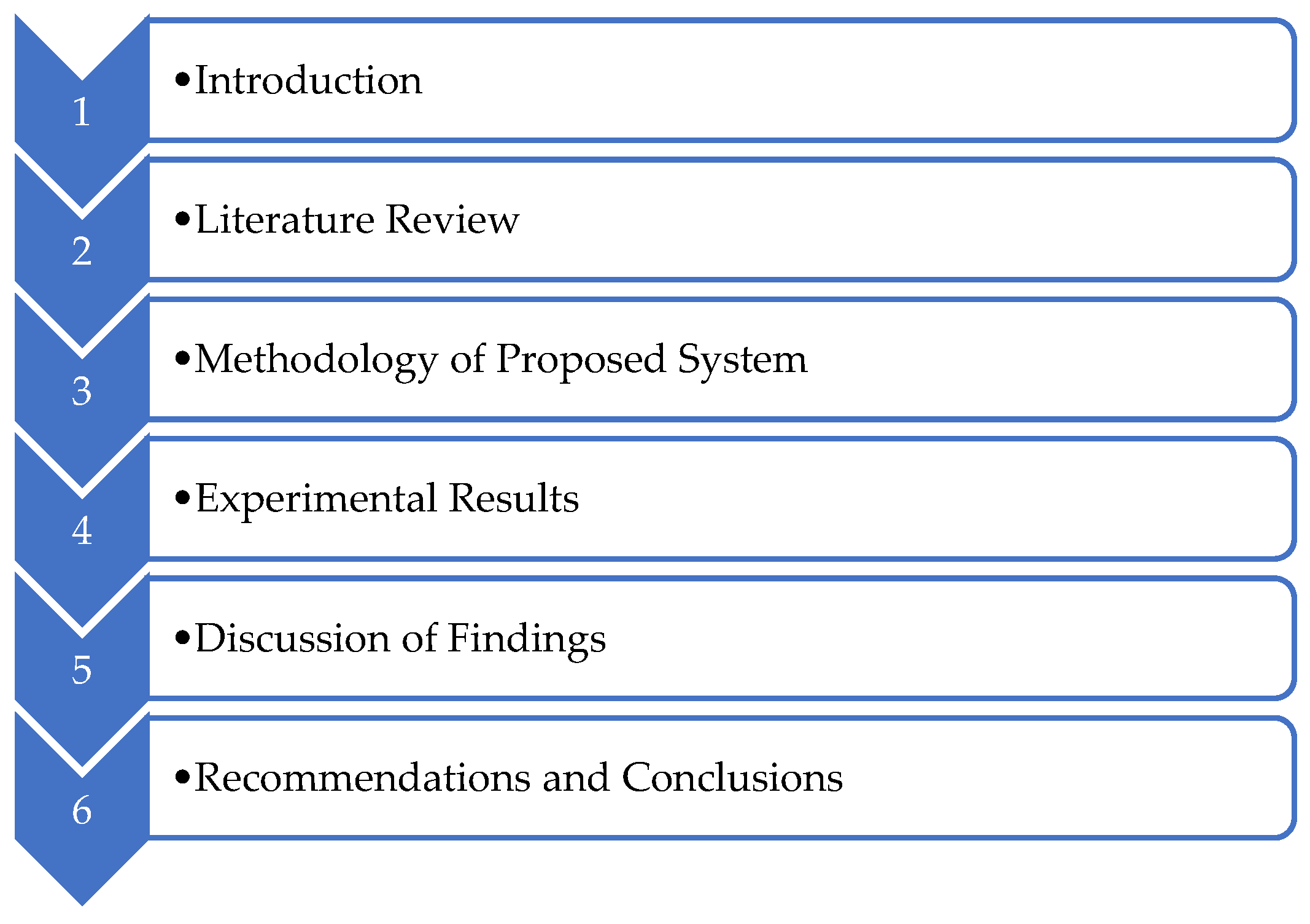
Figure 2.
Overall procedures for the analysis of forecasting include six steps.
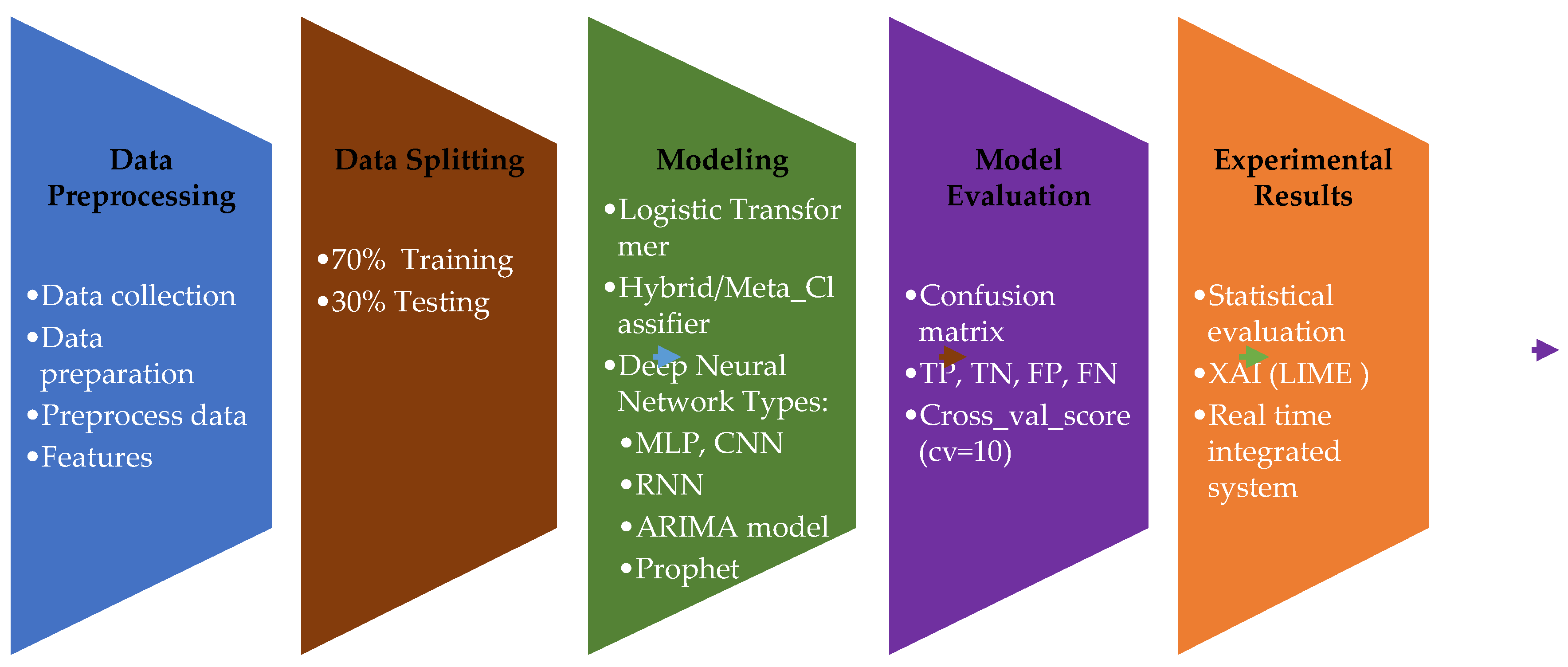
Figure 3.
Four steps make up the data preprocessing phase.

Figure 4.
Analysis of 175 features in data from remote sensing.
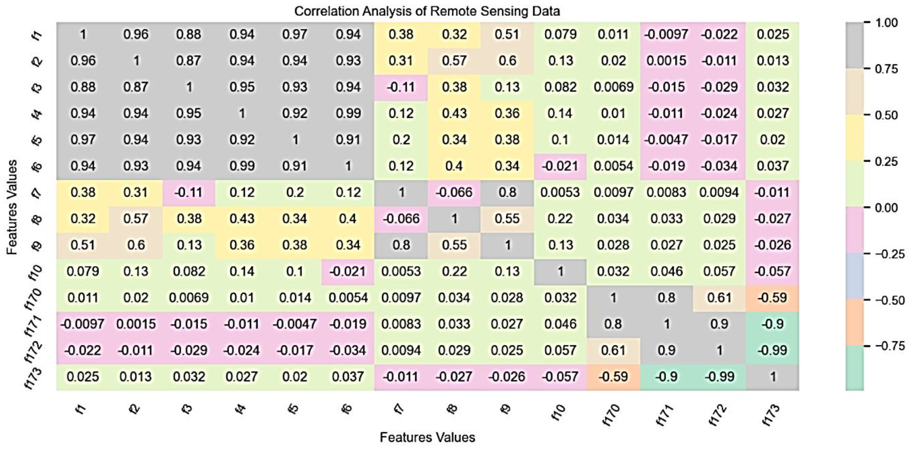
Figure 5.
Analysis of associations between the area and the hg/ha_yield prediction.
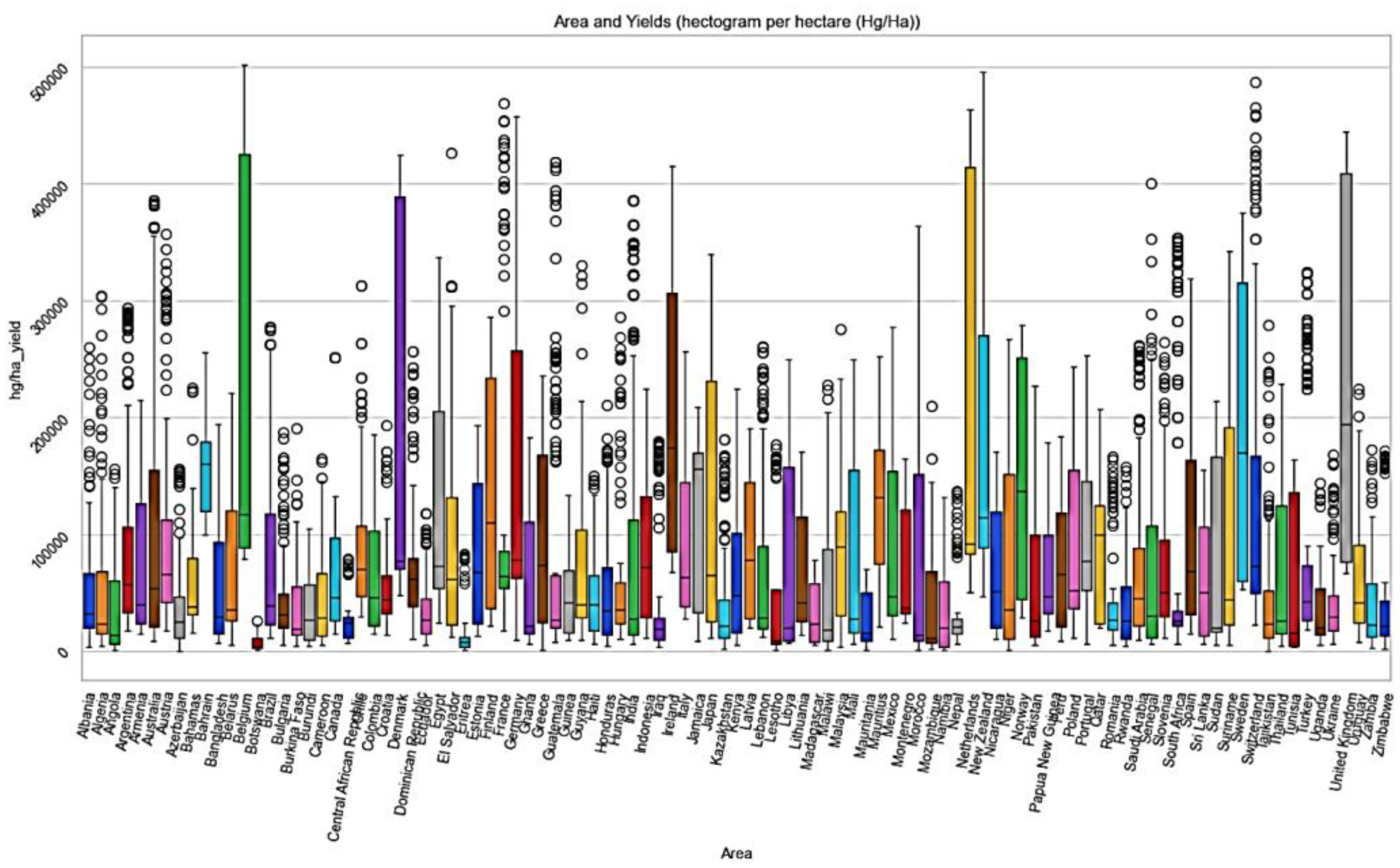
Figure 6.
The price distribution covers the years from 2008 to 2024. .
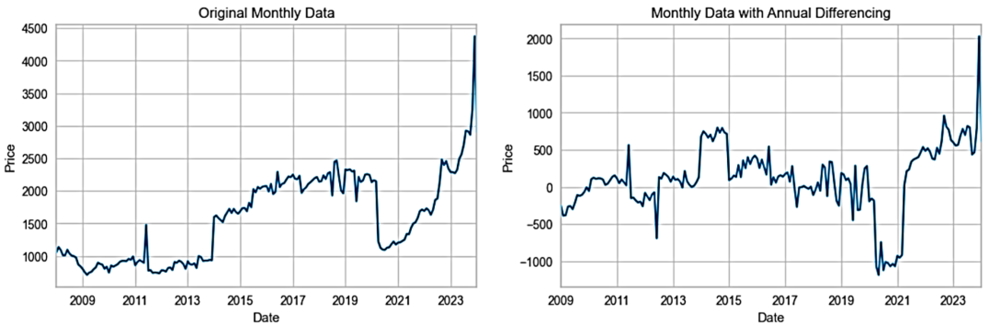
Figure 7.
Regression using Logistic Regression Architecture.
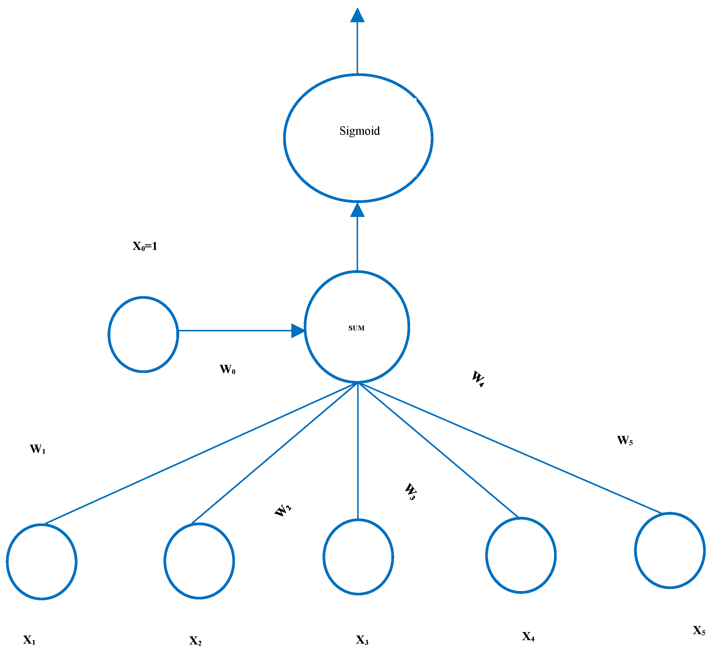
Figure 8.
Hybrid model architecture for yield prediction.
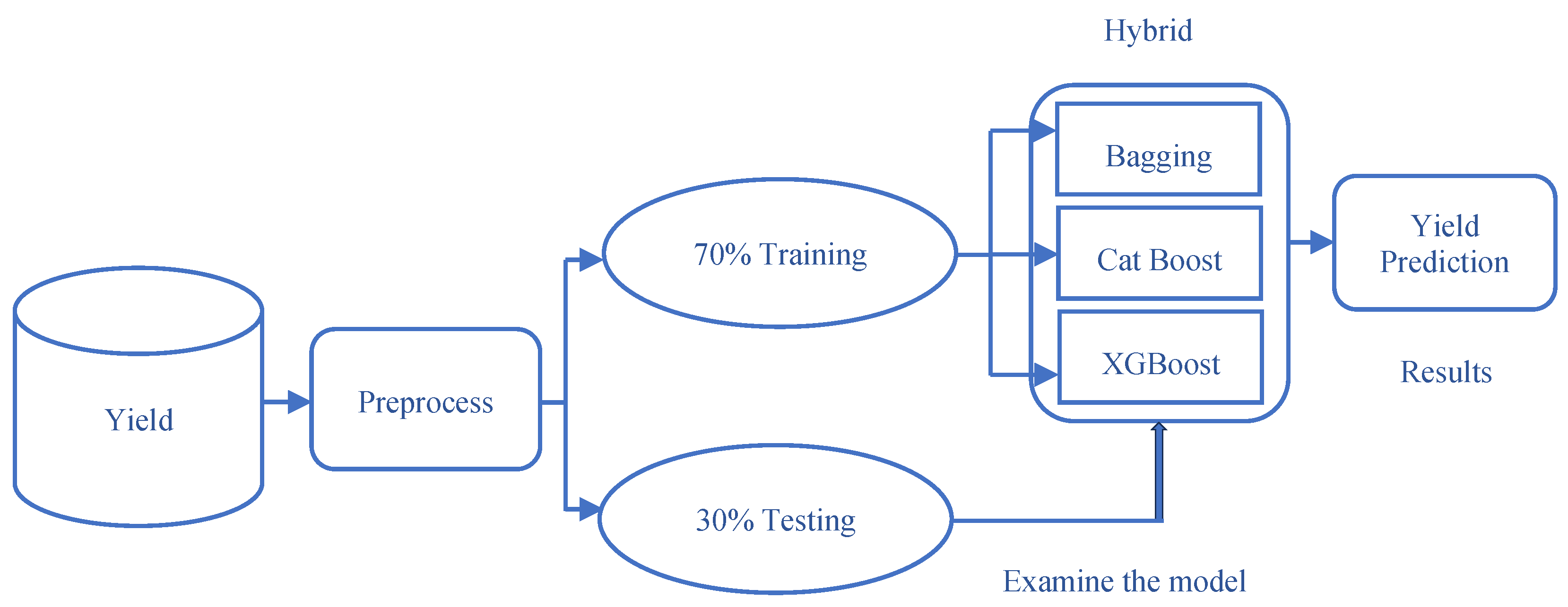
Figure 9.
Process for predicting prices using both conventional algorithms and deep learning models.
Figure 9.
Process for predicting prices using both conventional algorithms and deep learning models.
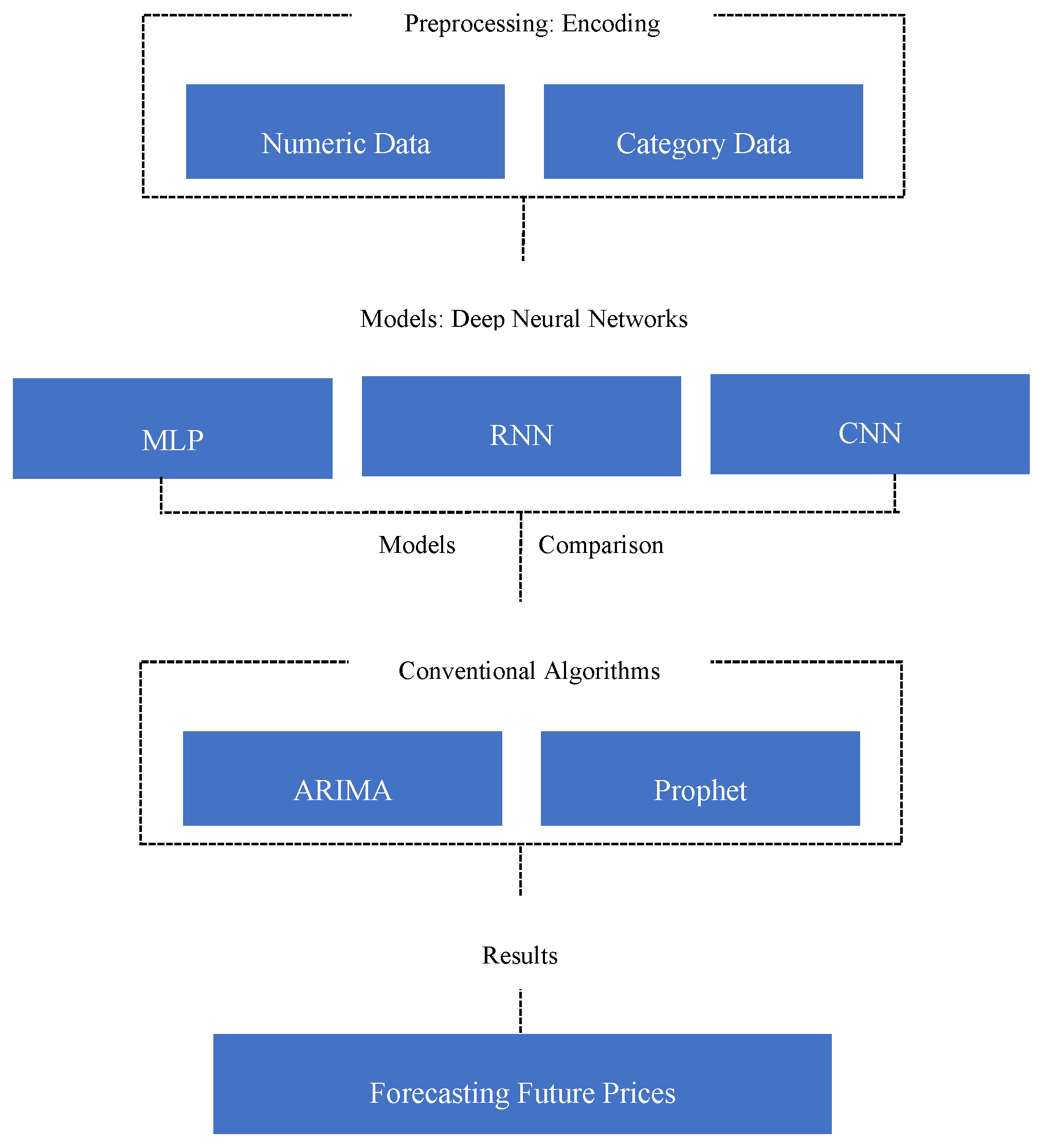
Figure 10.
Ten-time cross-validation of K-fold systems of all kinds.
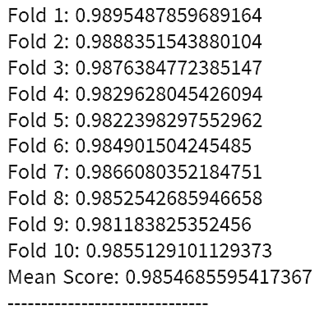
Figure 11.
Predicting yield products with the Meta Classifier.
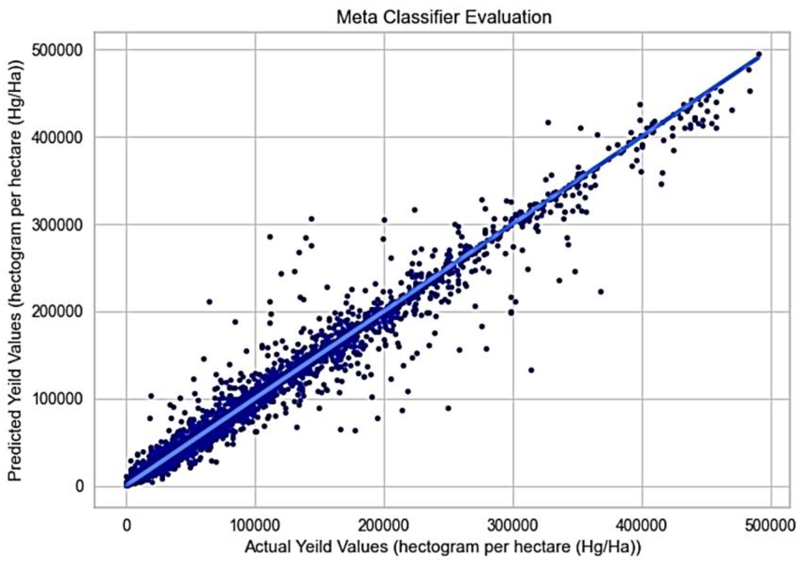
Figure 12.
CNN, RNN, and MLP models based on future price forecasting.
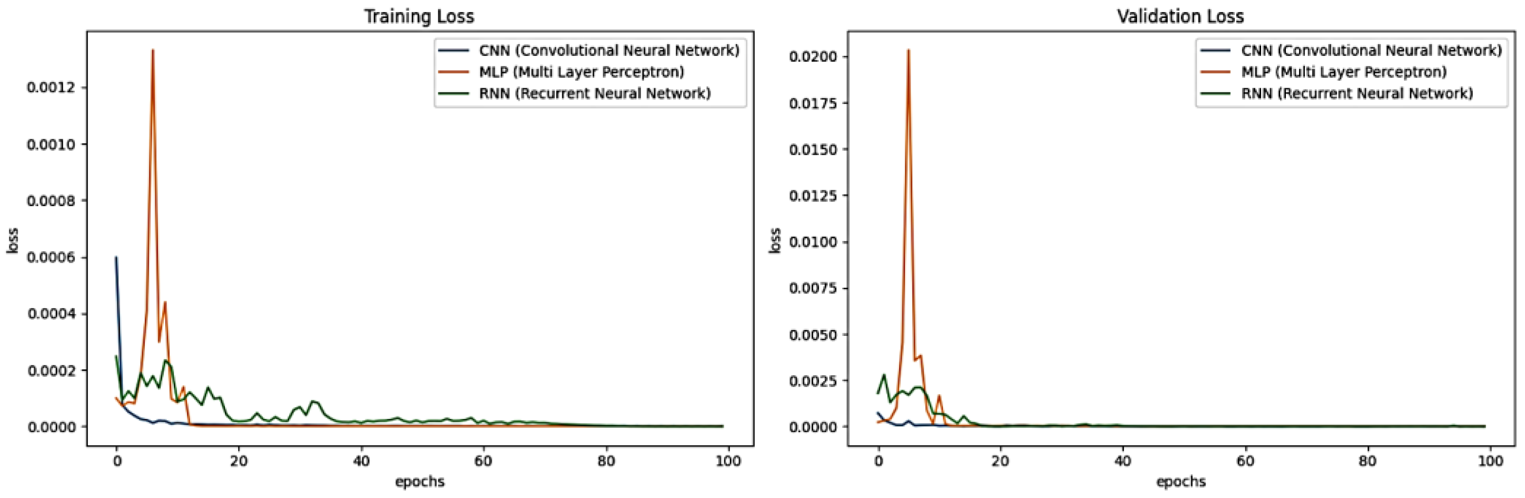
Figure 14.
LIME results for crop recommendation.
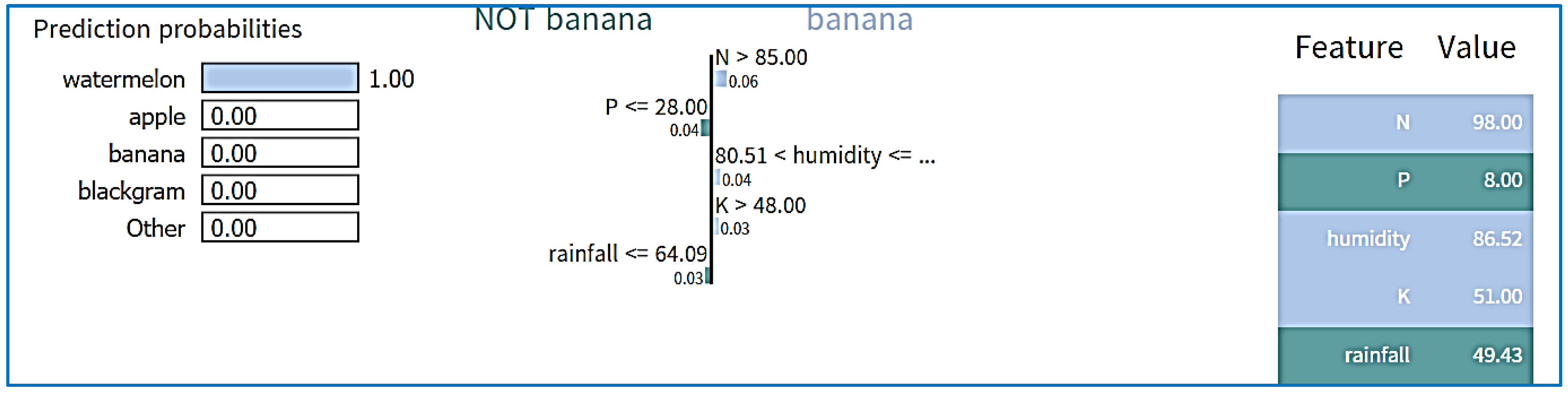
Figure 15.
Yield prediction’s LIME outputs.
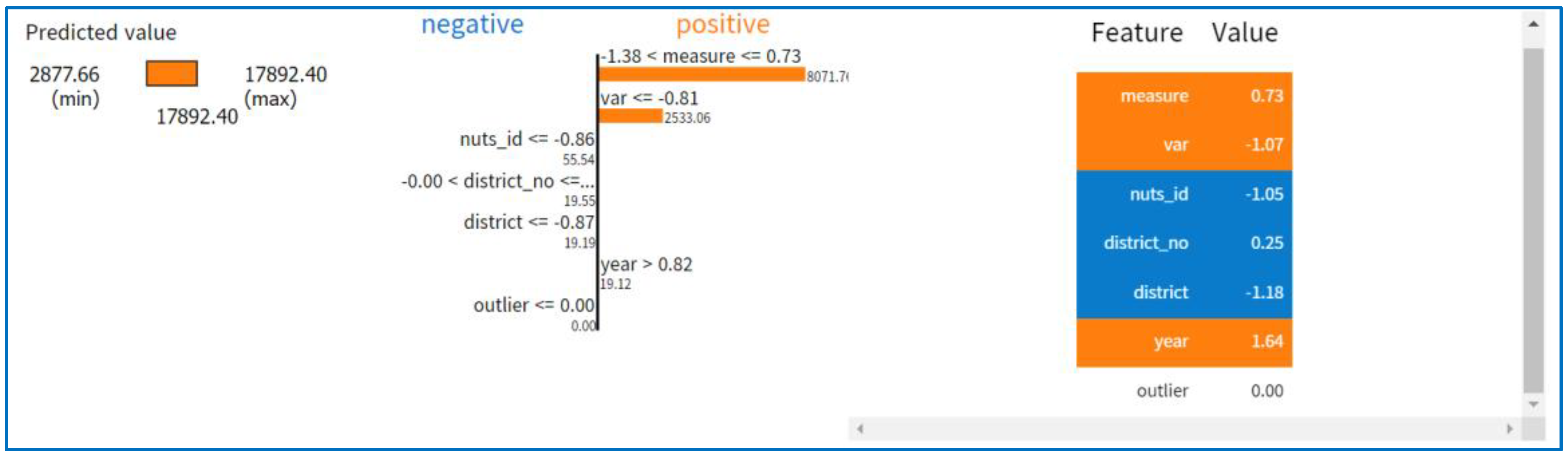
Figure 16.
LIME outcomes for price forecasting.
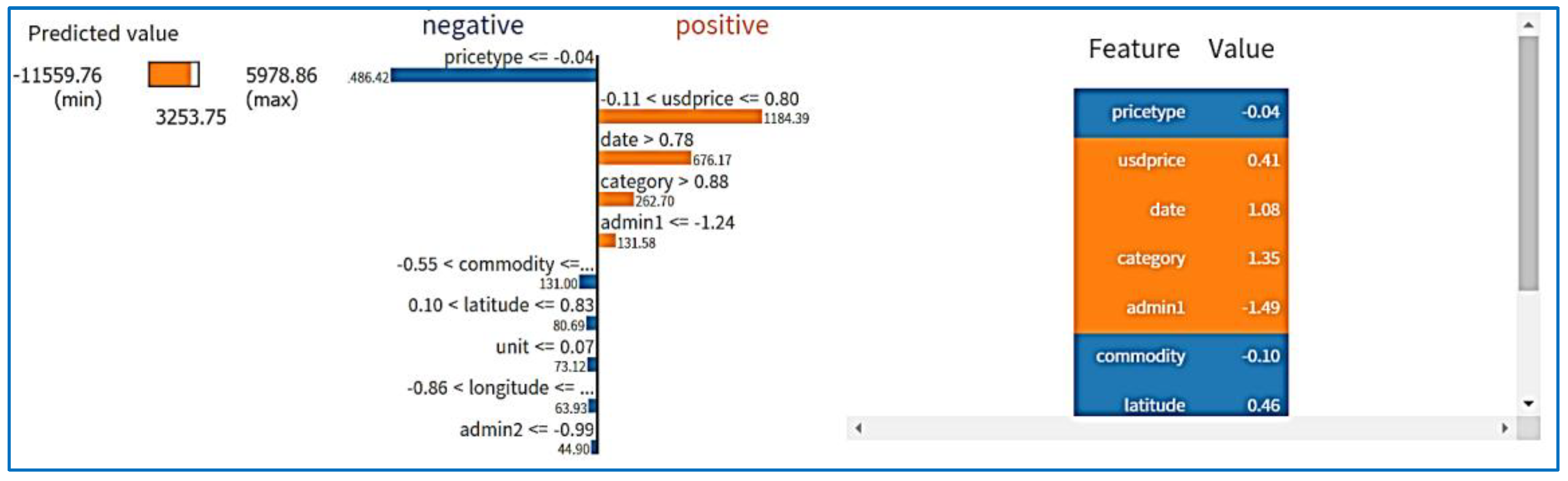
Figure 17.
Integrated into the design of an agricultural system.
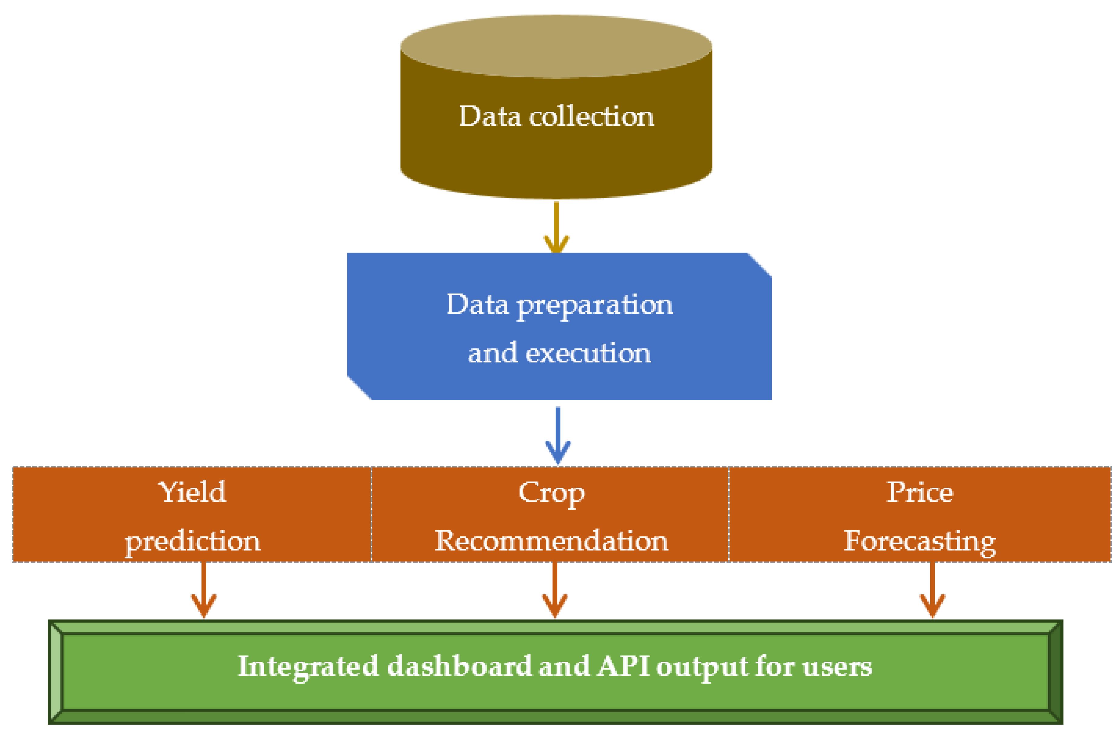
Figure 18.
AI-powered dashboard.
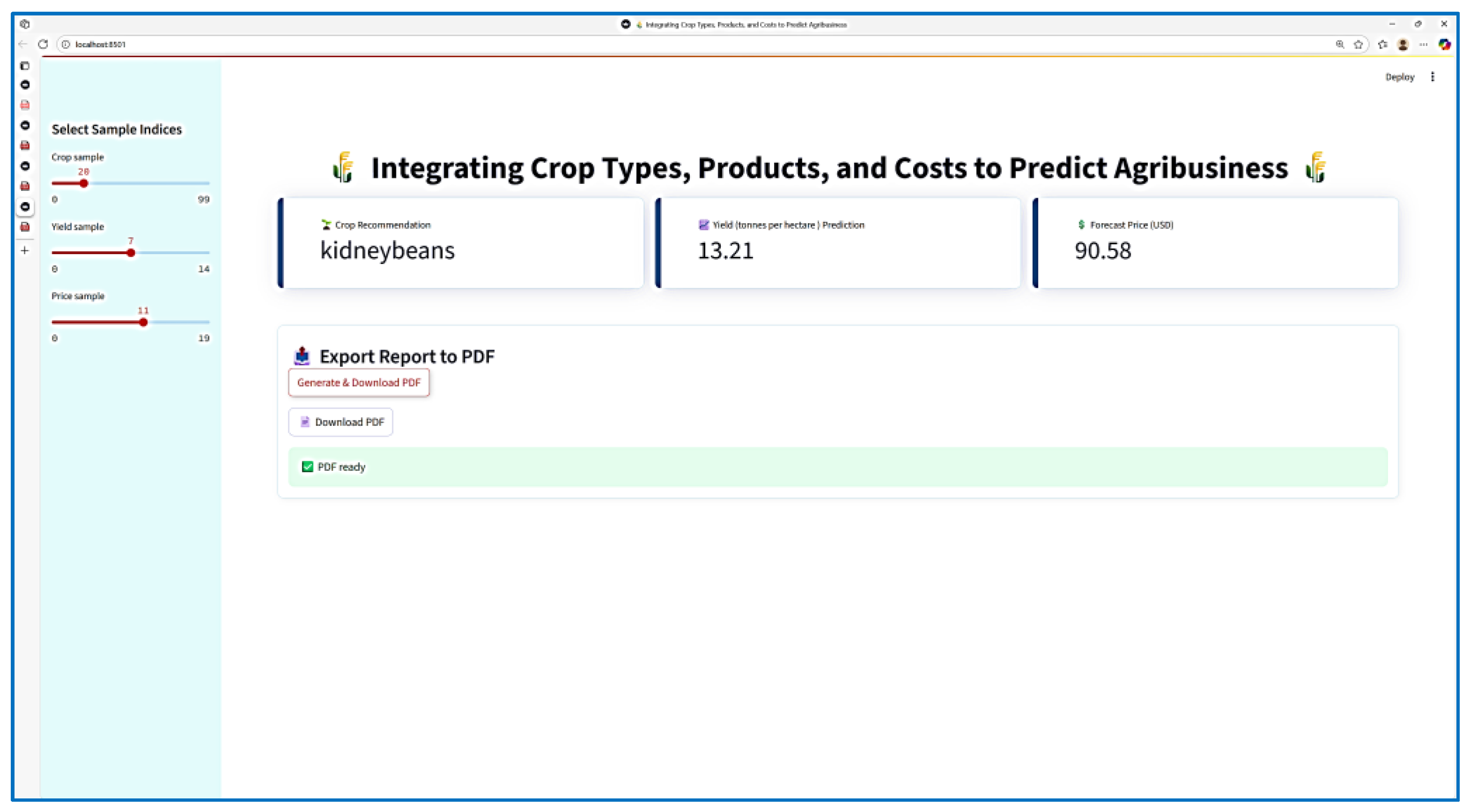
Figure 19.
PDF dashboard report.
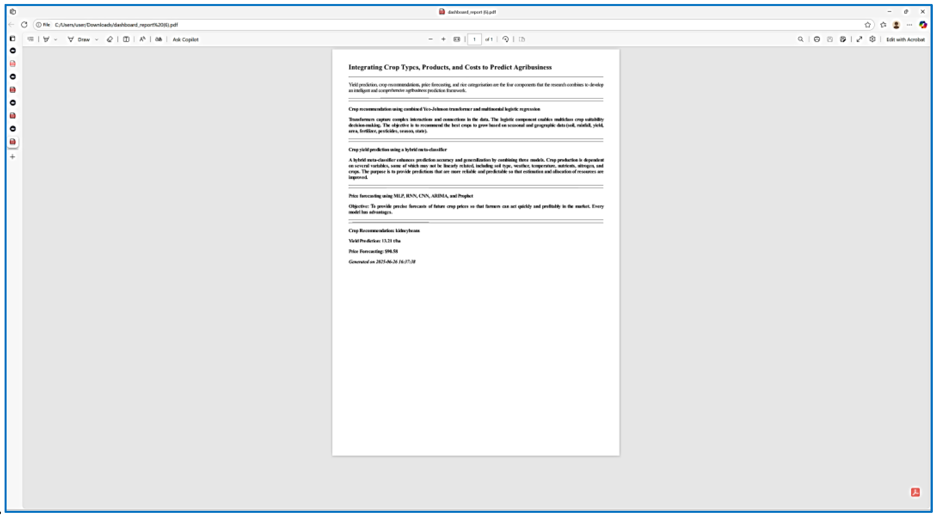
Table 1.
Six of the datasets were used.
| Task | Data Size | Model Type |
|---|---|---|
| Crop Recommendation |
2220 rows (ICFA) | combined Yeo-Johnson transformer and multinomial logistic regression + XAI (SHAP) + Real-time |
| 325,834 data points (UCI) | ||
| Yield Prediction | 259815 rows (German yield) | Hybrid Model +XAI (SHAP) + Real-time |
| 19689 entries (FAO) | ||
| Price Forecasting | 171 rows (United Nations) | Deep learning techniques + XAI (SHAP) + Real-time |
| 47223 entries (World Food) |
Table 2.
Sample dataset for price forecasting.
| date | admin1 | admin2 | market | latitude | longitude | category | commodity | unit | price flag |
price type |
currency | price | USD price |
|---|---|---|---|---|---|---|---|---|---|---|---|---|---|
| 1/15/2008 | Kachin | Myitkyina | Wai Maw | 25.34222 | 97.44001 | cereals and tubers | Rice (low quality) | KG | actual | Retail | MM K |
400 | 63.0785 |
| 1/15/2008 | Kachin | Myitkyina | Wai Maw | 25.34222 | 97.44001 | meat, fish, and eggs | Meat (chicken) | KG | actual | Retail | MMK | 3636.36 | 573.4413 |
| 1/15/2008 | Kachin | Myitkyina | Wai Maw | 25.34222 | 97.44001 | meat, fish, and eggs | Meat (pork) | KG | actual | Retail | MMK | 3636.36 | 573.4413 |
| 1/15/2008 | Kachin | Myitkyina | Wai Maw | 25.34222 | 97.44001 | miscellaneous food | Salt | KG | actual | Retail | MMK | 242.42 | 38.2294 |
| 1/15/2008 | Kachin | Myitkyina | Wai Maw | 25.34222 | 97.44001 | vegetables and fruits | Onions | KG | actual | Retail | MMK | 969.7 | 152.9177 |
Table 3.
A sample of the FAOSTAT price forecasting dataset.
| Domain Code |
Domain | Area Code (M49) |
Area | Year Code |
Year | Item Code |
label | Months Code | Months | Element Code |
|---|---|---|---|---|---|---|---|---|---|---|
| CP | Consumer Price Indices |
36 | Australia | 2020 | 2020 | 23013 | Consumer Prices, Food Indices |
7001 | January | 6125 |
| CP | Consumer Price Indices |
36 | Australia | 2020 | 2020 | 23013 | Consumer Prices, Food Indices |
7002 | January | 6125 |
| CP | Consumer Price Indices |
36 | Australia | 2020 | 2020 | 23013 | Consumer Prices, Food Indices |
7003 |
January | 6125 |
| CP | Consumer Price Indices |
36 | Australia | 2020 | 2020 | 23013 | Consumer Prices, Food Indices |
7003 |
January | 6125 |
| CP | Consumer Price Indices |
36 | Australia | 2020 | 2020 | 23013 | Consumer Prices, Food Indices |
7003 |
January | 6125 |
Table 4.
A sample of the Remote Sensing data.
| Label | f1 | f2 | f3 | f4 | f5 | … | f171 | f172 | f173 |
|---|---|---|---|---|---|---|---|---|---|
| 1 | -12.676 | -19.051 | -9.1362 | -12.962 | -10.5520 | … | 0.00000 | -0.00000 | 1.00000 |
| 5 | -12.595 | -19.695 | -14.0660 | -16.776 | -11.8360 | … | 0.33333 | 0.84869 | 0.50617 |
| 4 | -17.026 | -26.219 | -15.6050 | -19.435 | -16.2890 | … | 0.00000 | -0.00000 | 1.00000 |
Table 5.
Cropy yield dataset attributes.
Numerical Attributes:
|
Categorical Attributes:
|
Table 6.
Crop yield dataset variable.
| Variable | Description |
|---|---|
| Area | Names of nations that cultivate crops. |
| Item | Varieties of crops that were planted. |
| Year | Crop planting periods from 1990 to 2013. |
| average_rain_fall_mm_per_year | Annual rainfall average. |
| pesticides_tonnes | There are many tones for using pesticides. |
| avg_temp | Normal temperature. |
| hg/ha_yield | Value of production from crops expressed in hectograms per hectare (Hg/Ha). |
Table 7.
Crop yield dataset sample.
| Area | Item | Year | hg/ha_ yield |
average_rain_fall_ mm_per_year |
pesticides_ tonnes |
avg_temp |
|---|---|---|---|---|---|---|
| Albania | Maize | 1990 | 36613 | 1485 | 121 | 16.37 |
| Albania | Potatoes | 1990 | 66667 | 1485 | 121 | 16.37 |
| Albania | Rice, paddy | 1990 | 23333 | 1485 | 121 | 16.37 |
| Albania | Sorghum | 1990 | 12500 | 1485 | 121 | 16.37 |
| Albania | Soybeans | 1990 | 7000 | 1485 | 121 | 16.37 |
Table 8.
The German yield dataset sample.
| district_no | district | nuts_id | year | var | measure | value | outlier |
|---|---|---|---|---|---|---|---|
| 1001 | Flensburg, kreisfreie Stadt | DEF01 | 1979 | ArabLand | area | 891.0 | 0 |
| 1001 | Flensburg, kreisfreie Stadt | DEF01 | 1979 | district | area | 5673.0 | 0 |
| 1001 | Flensburg, kreisfreie Stadt | DEF01 | 1979 | grain_maize | area | NaN | 0 |
| 1001 | Flensburg, kreisfreie Stadt | DEF01 | 1979 | grain_maize | yield | NaN | 0 |
| 1001 | Flensburg, kreisfreie Stadt | DEF01 | 1979 | oats | yield | 42.0 | 0 |
Table 9.
Values of a Logistic Transformer model's hyperparameters for crop recommendation.
| Hyperparameter | Value/Description |
|---|---|
| Model Type | Logistic Transformer |
| Input Features | optical-radar data, crop types, satellite images |
| Number of Features | f174 |
| variance_inflation_factor | variable, i |
| random_state | 2 |
| Feature Scaling | X_train, X_test |
| cross-validation score | cv=5 |
| Mean cross-validation accuracy | cv_scores.mean() |
| Evaluation Metrics | Accuracy, Precision, Recall, F-Score, |
Table 10.
Summary of Multi-Layer Perceptron (MLP) parameters.
| Layer (type) dense_14 (Dense) dense_15 (Dense) dense_16 (Dense) |
Output Shape (None, 100) (None, 50) (None, 3) |
Parameters 2500 5050 153 |
| Total parameters: Trainable parameters: Non-trainable parameters: |
7703 7703 0 |
Table 11.
The architecture of the CNN model.
| Step 1 | The input data's form is first specified by defining an input layer. |
| Step 2 | The CNN architecture is then defined by building a sequential model. |
| Step 3 |
This stage involves adding three convolutional layers to the sequential model, each consisting of a convolutional layer, a max-pooling layer, and a flattening layer. |
| Step 4 | Step 4 involves flattening the convolutional layers' output, which turns the 2D matrix data into a 1D vector. Two completely linked layers are subsequently fed this flattened representation. Lastly, the output layer is the final layer. |
| Step 5 | Finally, the inputs and outputs are specified to construct the model. |
Table 12.
Construction of the RNN model.
|
# Define the RNN model model = Sequential( ) model.add(RNN(50, activation='relu', input_shape=(n_steps, n_features))) model.add(BatchNormalization()) model.add(Dense(n_out)) # Compile and Fit the model model_rnn.compile(loss='mse', optimizer='adam', metrics=['mae', 'mape', RootMeanSquaredError( ), RSquare( )]) hist_rnn = model_rnn.fit (x_train, y_train, validation_data=(x_valid, y_valid), shuffle=False, epochs=100, batch_size=32, verbose=2) # Demonstrate prediction eval_rnn = model_rnn.evaluate(x=x_test, y=y_test, return_dict=True) |
Table 13.
The ARIMA's pseudocode steps.
| INPUT: Time series data Determine p, d, and q (ARIMA parameters) - For MA order (q), plot the Autocorrelation (ACF) - Plot the AR order (p) Partial Autocorrelation (PACF) SET p = from PACF or user-defined SET d = total number of applied differences SET q = specified by the user from ACF MODEL: ARIMA (order=(p, d, q)) for time series data FIT model = model fit Assess the model Predict future values Results of output |
Table 14.
The ARIMA and Prophet price forecasting hyperparameter values.
| Price Forecasting Models | Hyperparameter Values Explanation |
|---|---|
| ARIMA parameters | p, d, and q |
| p | PACF (Partial Autocorrelation) or user-defined |
| d | total number of applied differences |
| q | specified by the user from ACF (Autocorrelation) |
| Prophet parameters | seasonality, change points, and missing data |
| seasonality mode | additive |
| uncertainty samples | 1000 |
| Changepoint prior scale | 0.05 |
Table 15.
Logistic transformer accuracy comparison.
| Proposed Models |
Range Index |
Training Accuracy |
Testing Accuracy |
|---|---|---|---|
| Combining Yeo-Johnson transformer and multinomial logistic regression with Remote Sensing Data |
325,834
data points |
0.986873 | 0.984877 |
| Logistic Transformer with Crop Data | 2200 entries | 0.773000 | 0.713524 |
Table 16.
Accuracy comparisons between the proposed logistic transformer algorithm and earlier studies [4].
Table 16.
Accuracy comparisons between the proposed logistic transformer algorithm and earlier studies [4].
| Algorithms | Accurateness |
|---|---|
| Recommendation using Remote Sensing Data Recommendation using Crop Data |
98% 71% |
| Multivariate Linear Regression (MLR) [4] Support Vector Machine (SVM) [4] Artificial Neural Network (ANN) [4] K Nearest Neighbor (KNN) [4] Random Forest (RF) [4] |
60% 75% 86% 90% 95% |
Table 19.
Deep learning models with price forecasting capabilities.
| Models | Loss | MAE | MAPE | RMSE | R squared |
|---|---|---|---|---|---|
| MLP | 0.019 | 0.016 | 0.440 | 0.139 | 0.985 |
| CNN | 0.019 | 0.019 | 0.596 | 0.138 | 0.985 |
| RNN | 0.015 | 0.016 | 0.486 | 0.124 | 0.988 |
Disclaimer/Publisher’s Note: The statements, opinions and data contained in all publications are solely those of the individual author(s) and contributor(s) and not of MDPI and/or the editor(s). MDPI and/or the editor(s) disclaim responsibility for any injury to people or property resulting from any ideas, methods, instructions or products referred to in the content. |
© 2025 by the authors. Licensee MDPI, Basel, Switzerland. This article is an open access article distributed under the terms and conditions of the Creative Commons Attribution (CC BY) license (http://creativecommons.org/licenses/by/4.0/).
Copyright: This open access article is published under a Creative Commons CC BY 4.0 license, which permit the free download, distribution, and reuse, provided that the author and preprint are cited in any reuse.


