

Submitted:
11 July 2025
Posted:
14 July 2025
You are already at the latest version
Abstract
Wind waves are generally considered to be surface gravity waves caused by wind and propagating under the restoring force of gravity. These waves have maximum particle motion right at the air-sea interface, the particle motion decreases rapidly with depth. They are distributed over most of the ocean, with long waves propagating faster than short waves. The research method used for this study is quantitative analysis, namely from secondary data (wind speed and direction data) in the Cermin Beach area using the Jonswap Parameters, Finite Water Depth and Sverdrup Munk Bretschneider methods. From the analysis results using the Windrose diagram, the dominant wind direction is 345°-15° with a percentage of 21.03%. For the Jonswap Parameters method, the maximum wave height and period are 0.906 m and 9.911 seconds. In the Finite Water Depth method, the maximum wave height and period for a depth of 3 meters are 1.304 m and 4.785 seconds, while at a depth of 10 meters they are 2.048 m and 6.743 seconds. In the Sverdrup Munk Bretschneider method, the maximum wave height and period for incomplete waves (Fetch Limited) are 1.815 m and 5.653 seconds, while for full waves (Fully Developed) they are 1.857 m and 5.750 seconds. In the results of the wave statistical return period, the maximum height results that occurred in the 100-year return period were obtained at a height of 10,445 m using the Gumbel method calculation with wave data from the Finite Water Depth method at a depth of 10 meters.
Keywords:
wind waves
; windrose
; Jonswap parameters
; finite water depth
; Sverdrup Munk Bretschneider
; return period
1. Introduction
Of the various types of wave motions that may occur in the ocean, wind waves are among the most energetic and easily observed. Therefore, one of the most studied waves is wind waves. Wind waves are generally considered to be surface gravity waves caused by wind and propagating under the restoring force of gravity. These waves have a maximum particle motion right at the air-sea interface, the particle motion rapidly decreasing with depth. They are distributed over most of the ocean, with long waves propagating faster than short waves.
Therefore, the behavior of waves generated by wind must be recorded every day in order to obtain their characteristic forms which will be useful in the future, both in research and in planning coastal building construction.
2. Materials and Methods
2.1. Wind
Wind, by definition, is the movement of air (primarily horizontal) in response to differences in air pressure caused primarily by differences in heating and cooling [1].
Wind data can be obtained from the nearest meteorological station or from the nearest airport. The data obtained is usually classified so that further data processing can be simpler and in general the data is sorted based on the distribution of wind speed and direction, as well as its percentage or known as windrose which can be seen in Figure 1.
The wind speed in wave forecasting calculations must be the wind speed over water. In general, it is only necessary to know the wind speed from the nearest airport, and we must take into account that the wind over water is usually greater than the wind over land because of the smaller friction on the water. Therefore, a transformation of the wind data over land closest to the study location to the wind data over the sea surface is required.
The equation for wind speed that will be used for wave forecasting is:
U = RT . RL (U10)L
In this equation, RT represents the correction factor accounting for temperature differences between the air and water, as illustrated in Figure 2. RL denotes the correction applied to wind measurements taken on land, which is detailed in Figure 3. The term (U10)L refers to the wind speed measured at a height of 10 meters above ground level on land.
Correction between wind data on land and above sea level can use the following equation:
In this equation, the correction factor for wind speed on land, denoted as RL, is used to adjust the wind speed measured above sea level (UW) to its equivalent value over land (UL). This factor accounts for the differences in surface roughness and friction between the sea and land surfaces, which affect wind speed. Specifically, RL represents the ratio or relationship between the wind speed at sea and the wind speed observed over land, enabling more accurate assessments in meteorological and engineering applications.
The wind speed must be converted to the wind stress factor (UA) using the following equation:
UA = 0,71 U 1,23
In this equation, U represents the internal wind speed measured in meters per second. The variable UA denotes the wind stress factor, which influences the value of the internal wind speed.
2.2. Fetch
In wave generation at sea, Fetch (which can be seen in Figure 4) is limited by the shape of the land surrounding the sea. In the wave formation area, waves are not only generated in the same direction as the wind direction but also at various angles to the wind direction [2]. For Fetch equation:
In this equation, Feff represents the effective average fetch, which is a measure used to account for the varying distances over which wind blows across the water surface to generate waves. The term Xi refers to the length of each fetch segment, measured from the wave observation point to the end of the fetch in a specific direction. Meanwhile, ai denotes the angular deviation on both sides of the primary wind direction, calculated using predetermined angle increments up to the maximum angle considered on either side of the wind direction.
2.3. Wave
Waves in the sea can be divided into several types depending on the generating force. These waves are wind waves generated by wind blowing on the sea surface, tidal waves generated by the gravitational pull of celestial bodies, especially the sun and moon, tsunami waves caused by volcanic eruptions or earthquakes in the sea, waves generated by moving ships, and so on [2].
2.4. Jonswap Parameters
The Jonswap method for wave forecasting uses the following formula:
Then, for the Jonswap relationship, namely:
In this method, the dimensionless fetch length (F*) is based on the actual fetch length (F) and is normalized with respect to wind conditions. The dimensionless zero moment wave height (Hmo*) corresponds to zero moment wave height (Hmo), which represents the significant wave height derived from the wave energy spectrum. The dimensionless peak wave period (Tp*) is derived from the peak wave period (Tp), the period associated with the peak energy in the wave spectrum. The dimensionless duration (t*) is a scaled form of the actual duration (t) over which the wind acts. The dimensionless depth (d*) represents the normalized value of the water depth (d). All these parameters are typically normalized using the wind speed (U), which plays a critical role in wave generation and growth. Additionally, the concept of effective fetch (Feff*) is used to represent a modified fetch that accounts for wind direction variability or other influencing factors, and is also expressed in dimensionless form. These dimensionless parameters allow for scalable, comparative analysis of wave characteristics across different oceanographic and meteorological scenarios.
2.5. Finite Water Depth
Water depth affects wave formation. For a given wind condition and fetch length, the wave height will be smaller and the wave period shorter if the formation occurs in transitional or shallow waters than in deep waters [3]. For the calculation, the following formula is used:
In this method, several dimensionless parameters are used to describe wave characteristics. The dimensionless wave height is denoted by H*, while the dimensionless wave period is represented by T*. The dimensionless duration of wave generation is expressed as t*, and the dimensionless depth of the water is indicated by d*. These parameters are typically derived by normalizing their respective physical quantities with appropriate scaling factors, allowing for generalized analysis of wave behavior across different conditions.
2.6. Sverdrup Munk Bretschneider
The Sverdrup Munk Bretschneider (SMB) method is a method used to obtain significant sea wave height and period values. The SMB method calculation is formulated as follows:
2.6.1. Incomplete wave growth condition (Fetch Limited)
- Significant wave height (Hs);
- Significant wave period (Tm);
- Wind duration;
2.6.2. Full wave growth conditions (Fully Developed)
- Significant wave height (Hs);
- Significant wave period (Tm);
- Wind duration;
In this method, Hs represents the significant wave height, which is a measure of the average height of the highest one-third of waves. Tm refers to the wave period, indicating the time interval between successive wave crests. The term F denotes the fetch length, which is the distance over water that the wind blows in a single direction. UA is the wind stress factor, representing the influence of wind on the water surface. U stands for wind speed, while g is the gravitational acceleration, typically taken as 9.81 m/s2. Ts refers to the significant wave period, a specific measure related to Hs, and t indicates the duration for which the wind has been blowing over the fetch area.
2.7. Statistical Analysis of Waves
Long-term wave data analysis provides a theoretical distribution of the probability of occurrence of wave parameters over a number of years, this analysis is most often performed on long-term wave height data [4]. For calculations, it is done using the following equation:
- Normal Distribution;
- Log-Normal Distribution;
- Gumbel Distribution;
- Weibull Distribution;
In this calculation of wave height analysis, the variable H represents the wave height, which is a key parameter in oceanographic and coastal studies. The symbol P denotes the probability associated with a specific wave height occurrence. σ stands for the standard deviation of wave height, reflecting the variability or dispersion of wave heights from the mean. Z refers to the standard normal variate, a dimensionless value derived from the standard normal distribution used in probabilistic calculations. indicates the mean wave height, which is the average value of all recorded wave heights. Lastly, represents the variation or variance of wave height, quantifying the extent to which individual wave heights differ from the mean.
Then, to calculate the wave height with the return period for each distribution, the following equation is used:
- Normal Distribution;
- Log-Normal Distribution;
- Gumbel Distribution;
- Weibull Distribution;
In the given equation, represents the wave height corresponding to a specific return period, . The return period indicates the average time interval between occurrences of waves of a certain height or greater. denotes the mean wave height, while refers to the wave variance spectral density function, which characterizes the distribution of wave energy over frequencies. The symbol P stands for probability, often associated with the likelihood of exceeding a certain wave height. The parameters and are shape and scale parameters, respectively, commonly used in Gumbel and Weibull distributions to statistically model extreme wave heights.
3. Results
3.1. Hydro-Oceanography Analysis (Wind)
3.2. Fetch Length
The wind directions that affect this beach are Northwest, North, Northeast and East. In the Southeast direction it does not have a direct effect, but it allows for a deflection towards Pantai Cermin and affects the morphology of the beach. By drawing a long line from Pantai Cermin, the Fetch length with the Northwest, North, Northeast, East and Southeast generation areas. The Fetch length can be seen in Table 2.
3.3. Determining Wave Height and Period
To forecast wave height, wind data is required which will then be processed using several deep sea wave forecasting equations, some of these equations are Jonswap Parameters, Finite Water Depth and Sverdrup Munk Bretschneider. The results of the calculations can be seen in Table 3, Table 4, Table 5, Table 6 and Table 7. The Waverose diagram can be seen in Figure 6, Figure 7, Figure 8, Figure 9 and Figure 10.
3.4. Statistical Analysis of Waves
The results of the statistical analysis of the calculation of the wave recurrence period using the method of Normal Distribution, Log-Normal Distribution, Gumbel Distribution and Weibull Distribution which show the largest wave height in each equation can be seen in Table 8, Table 9, Table 10, Table 11 and Table 12.
4. Discussion
Based on the analysis of wind speed and direction data, the dominant wind direction at Cermin Beach is from 345° to 15° (North), with a frequency of 21.03%. Using the Jonswap Parameters method, the highest wave height and period were observed in March 2020, reaching 0.906 meters and 9.911 seconds. The Finite Water Depth method showed maximum wave characteristics in October 2023 with a wave height of 1.304 meters and period of 4.785 seconds at a depth of 3 meters, and in April 2022 with a height of 2.048 meters and period of 6.743 seconds at a depth of 10 meters. Meanwhile, the Sverdrup Munk Bretschneider (SMB) method recorded the highest wave height and period in non-full wave conditions in October 2019 (1.815 m, 5.653 s), and in full wave conditions, the highest wave height occurred in April 2022 (1.857 m), with the longest period in March 2022 (5.750 s).
For the 100-year return period analysis, the Jonswap Parameters method estimated a maximum wave height of 4.825 meters using the Weibull Distribution. The Finite Water Depth method predicted 100-year maximum wave heights of 5.244 meters at a depth of 3 meters and 10.445 meters at a depth of 10 meters using the Gumbel Distribution. The SMB method estimated maximum wave heights of 7.799 meters under incomplete wave conditions and 7.377 meters under full wave conditions, both using the Weibull Distribution. From these results, it can be concluded that the Jonswap Parameters method is the most suitable for wave forecasting at Cermin Beach, as the wave heights in the area are not categorized as extreme.
5. Conclusions
To obtain more accurate calculation results in future research, further analysis using a larger dataset is recommended, particularly by processing hourly wind data. Additionally, it is suggested to compare the analysis results using various methods, such as by employing wave forecasting models developed by institutions like BMKG or ant institution, to enhance the reliability and validity of the findings.
Author Contributions
Conceptualization, A.P.M. and I.M.B.; methodology, A.P.M.; software, E.P.B.; validation, A.P.M. and E.P.B; formal analysis, A.P.M.; investigation, I.M.B.; resources, A.P.M.; data curation, I.M.B.; writing—original draft preparation, I.M.B.; writing—review and editing, I.M.B. and E.P.B; visualization, I.M.B.; supervision, A.P.M.; project administration, A.P.M.; funding acquisition, A.P.M. All authors have read and agreed to the published version of the manuscript.
Funding
This research received no external funding
Institutional Review Board Statement
Not applicable
Informed Consent Statement
Not applicable
Data Availability Statement
The wind direction and speed data presented in the study are obtained from Meteorology, Climatology and Geophysics Agency (BMKG), Indonesia. (requested on 10 Juny 2024)
Conflicts of Interest
The authors declare no conflicts of interest.
References
- Tsinker, G. Handbook of Port and Harbor Engineering, 1st ed.; Springer New York: N.Y., United States of America, 1997. [Google Scholar]
- Triatmodjo, B. Teknik Pantai, 5th ed.; Beta Offset: Yogyakarta, Indonesia, 1999. [Google Scholar]
- Coastal Engineering Research Center. Shore Protection Manual, 4th ed.; US Army Corps of Engineers: Washington DC, United States of America, 1984. [Google Scholar]
- Kamphuis, J. Introduction to Coastal Engineering and Management, 1st ed.; World Scientific: Farrer Road, Singapore, 2000. [Google Scholar]
- Annenkov, S. Y., & Shrira, V. I. Evaluation of Skewness and Kurtosis of Wind Waves Parameterized by JONSWAP Spectra. Journal of Physical Oceanography 2014, 44, 1582–1594.
- Applequist, S. Wind Rose Bias Correction. Journal of Applied Meteorology and Climatology 2012, 51, 1305–1309. [Google Scholar] [CrossRef]
- Chow, V. Te, Maidment, D. R., Mays. Applied Hydrology, Int. ed.McGraw-Hill, Inc.: Texas, United States of America, 1988; pp. 1–294.
- Fedorov, A. V., & Melville, W. K. A Model of Strongly Forced Wind Waves. Journal of Physical Oceanography 2009, 39, 2502–2522.
- Gang, C., & Belcher, S. E. Effects of Long Waves on Wind-Generated Waves. Journal of Physical Oceanography 1999, 30, 2246–2256.
- Huddiankuwera, A. Deformasi Gelombang pada Pemecah Gelombang Sisi Miring Berongga. Disertation, Universitas Hasanuddin, Makassar, 21 December 2022.
- Janseen, P. A. E. M. Wave-Induced Stress and the Drag of Air Flow over Sea Waves. Journal of Physical Oceanography 1989, 19, 745–754. [Google Scholar] [CrossRef]
- Lamont-Smith, T., & Waseda, T. Wind Wave Growth at Short Fetch. Journal of Physical Oceanography 2008, 38, 1597–1606.
- Poddaeva, O., & Fedosova, A. Extreme Wind Speeds Analysis Using Extended Wind Rose Based on Statistic Methods. Energy Reports 2022, 8, 1177–1184.
- Pratama, A. (2018). Analisa Statistik Gelombang yang Dibangkitkan di Wilayah Pantai Cermin. Undergraduate Thesis, Universitas Sumatera Utara, Medan, April 2018.
- Purwanto, Tristanto, R., Handoyo, G., Trenggono, M., & Suryoputro, A. A. D. Analisis Peramalan dan Periode Ulang Gelombang di Perairan Bagian Timur Pulau Lirang, Maluku Barat Daya. Indonesian Journal of Oceanography 2020, 2, 80–89.
- Raihan, G., Siregar, S., Adiningsih, S., & Heryanto, Y. Easywave untuk Peramalan Data Gelombang Laut Berbasis Pemograman Python Dengan Metode Sverrup, Munk and Bretschneider (SMB) (Studi Kasus: Perairan Sungairaden, Kalimantan Timur). Jurnal Meteorologi Klimatologi Dan Geofisika 2020, 7, 20–29.
- Setiawan, E., Adrianto, D., Dharma, C. S., & Kurniawan, E. S. Pengolahan Gelombang Permukaan Laut Menggunakan Metode Sverdrup Munk Bretschneider (SMB) di Perairan Pulau Pabelokan. Jurnal HIDROPILAR 2016, 2, 133–146.
- Shemdin, O. H. Wind-Generated Current and Phase Speed of Wind Waves. Journal of Physical Oceanographysical 1972, 2, 411–419. [Google Scholar] [CrossRef]
- Shilo, E., Ashkenazy, Y., Rimmer, A., Assouline, S., & Mahrer, Y. Wind Spatial Variability and Topographic Wave Frequency. Journal of Physical Oceanography 2008, 38, 2085–2096.
- Sorensen, R. M. Basic Coastal Engineering, 2nd ed.; Springer New York: N.Y., United States of America, 1997; pp. 9–52. [Google Scholar]
- Wright, J. W. The Wind Drift and Wave Breaking. Journal of Physical Oceanography 1976, 6, 402–405. [Google Scholar] [CrossRef]
Figure 1.
Windrose.
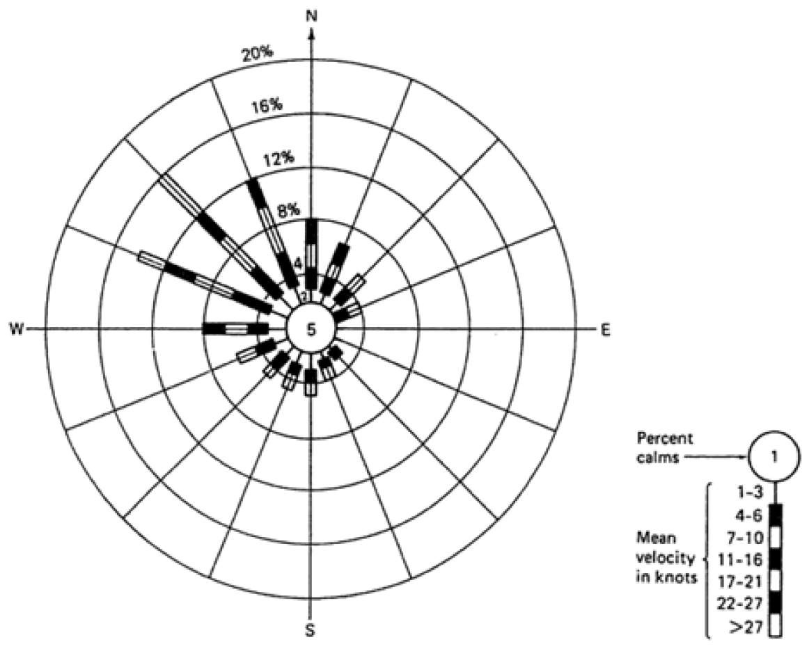
Figure 2.
Speed correction coefficient for temperature difference (RT).
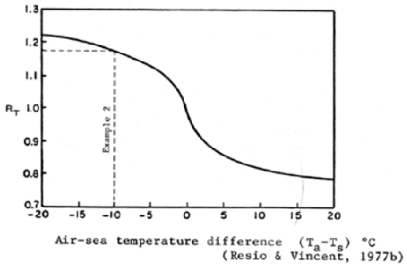
Figure 3.
Correction coefficient for ground speed recording (RL).
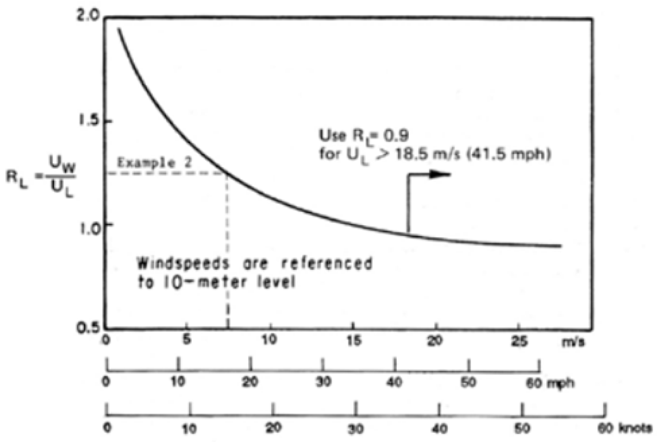
Figure 4.
Example of Fetch depiction.
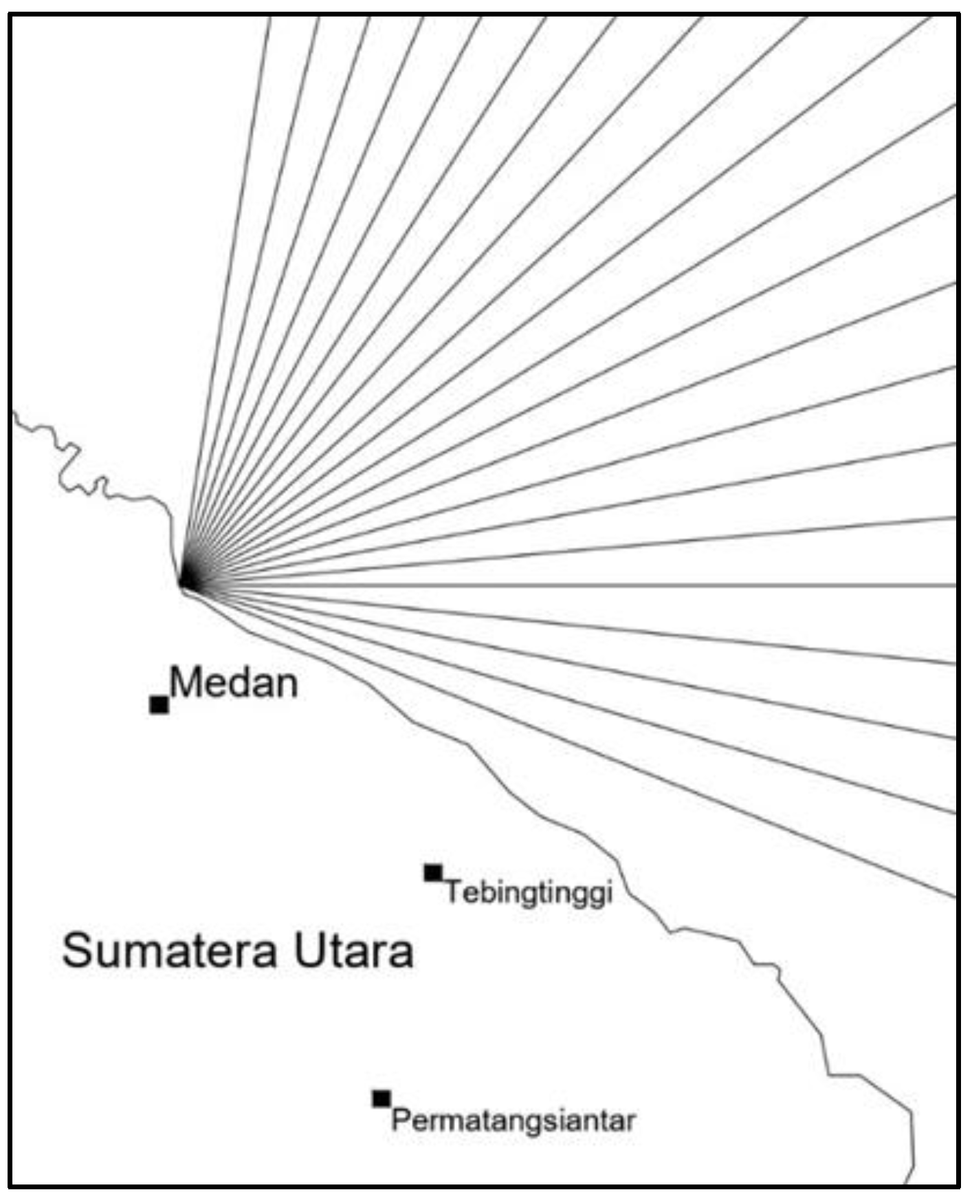
Figure 5.
Windrose Diagram on Cermin Beach from 2019 to 2023.
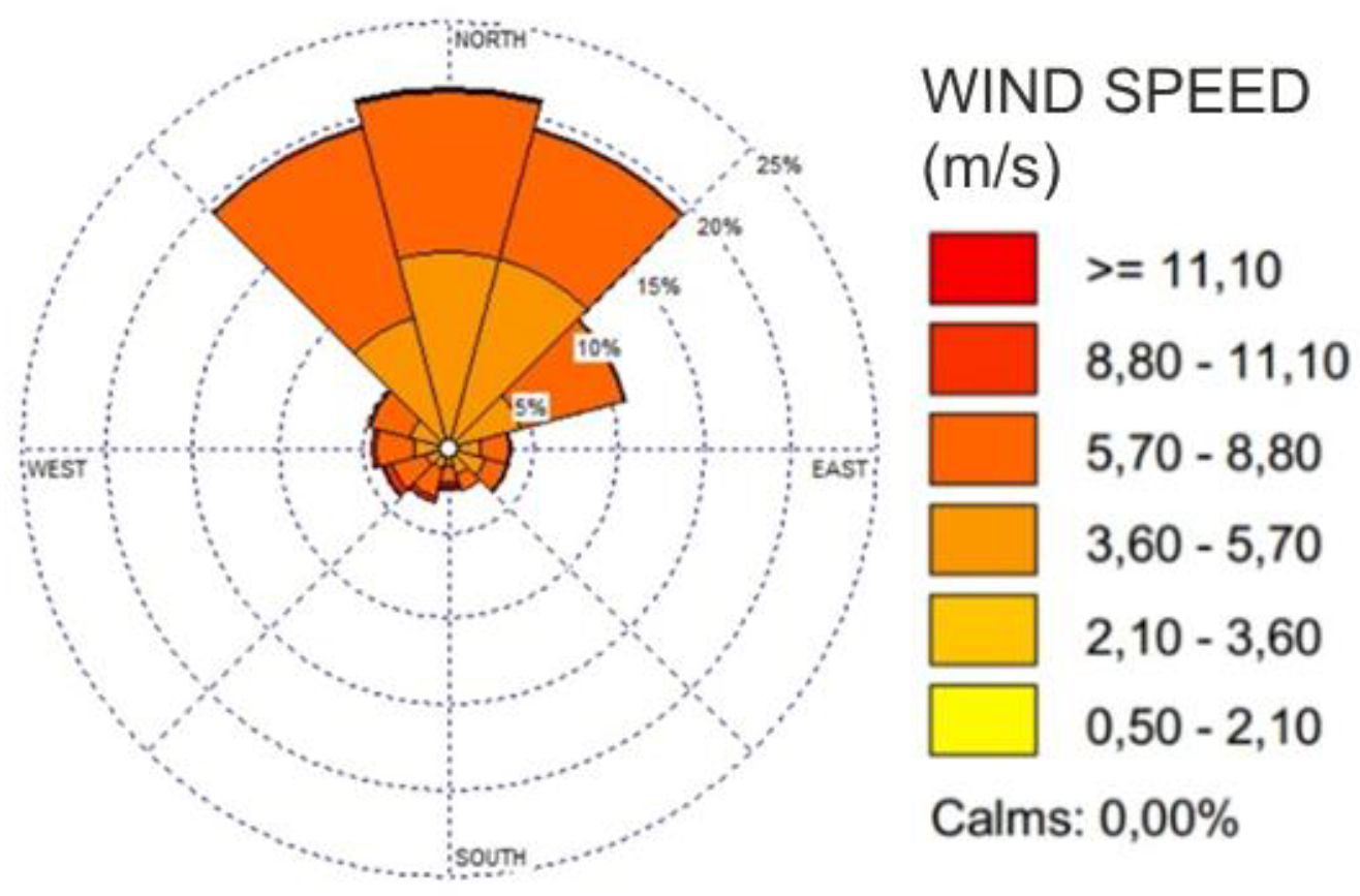
Figure 6.
Waverose Chart from 2019 to 2023 (Jonswap Parameters).
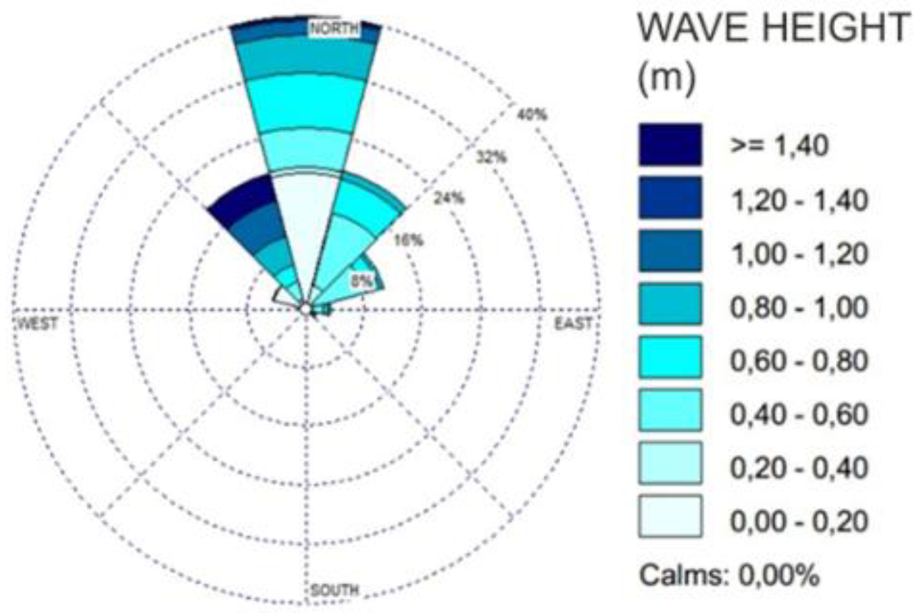
Figure 7.
Waverose Chart from 2019 to 2023 (Finite Water Depth, 3 meter).
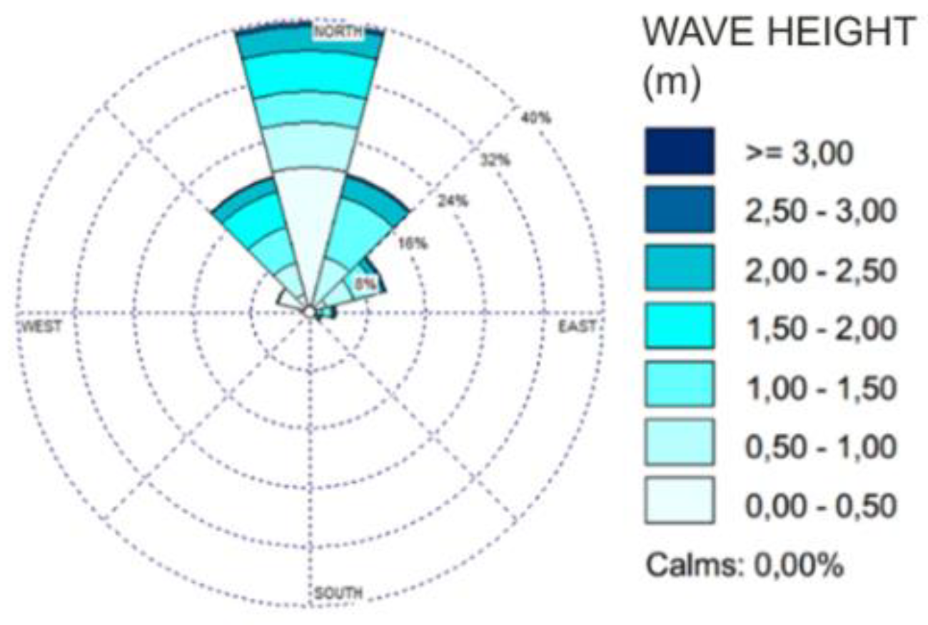
Figure 8.
Waverose Chart from 2019 to 2023 (Finite Water Depth, 10 meter).
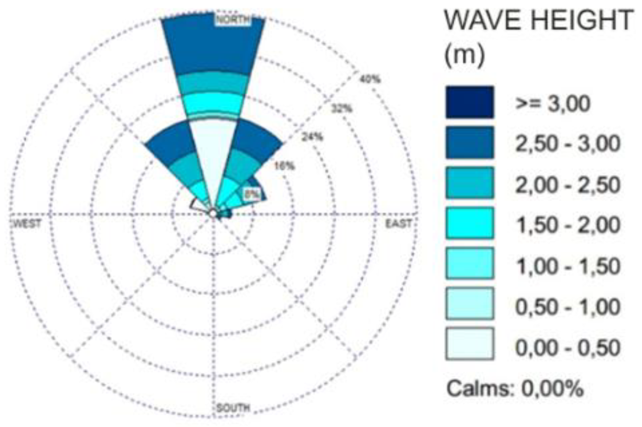
Figure 9.
Waverose Chart from 2019 to 2023 (Sverdrup Munk Bretschneider, Fetch Limited).
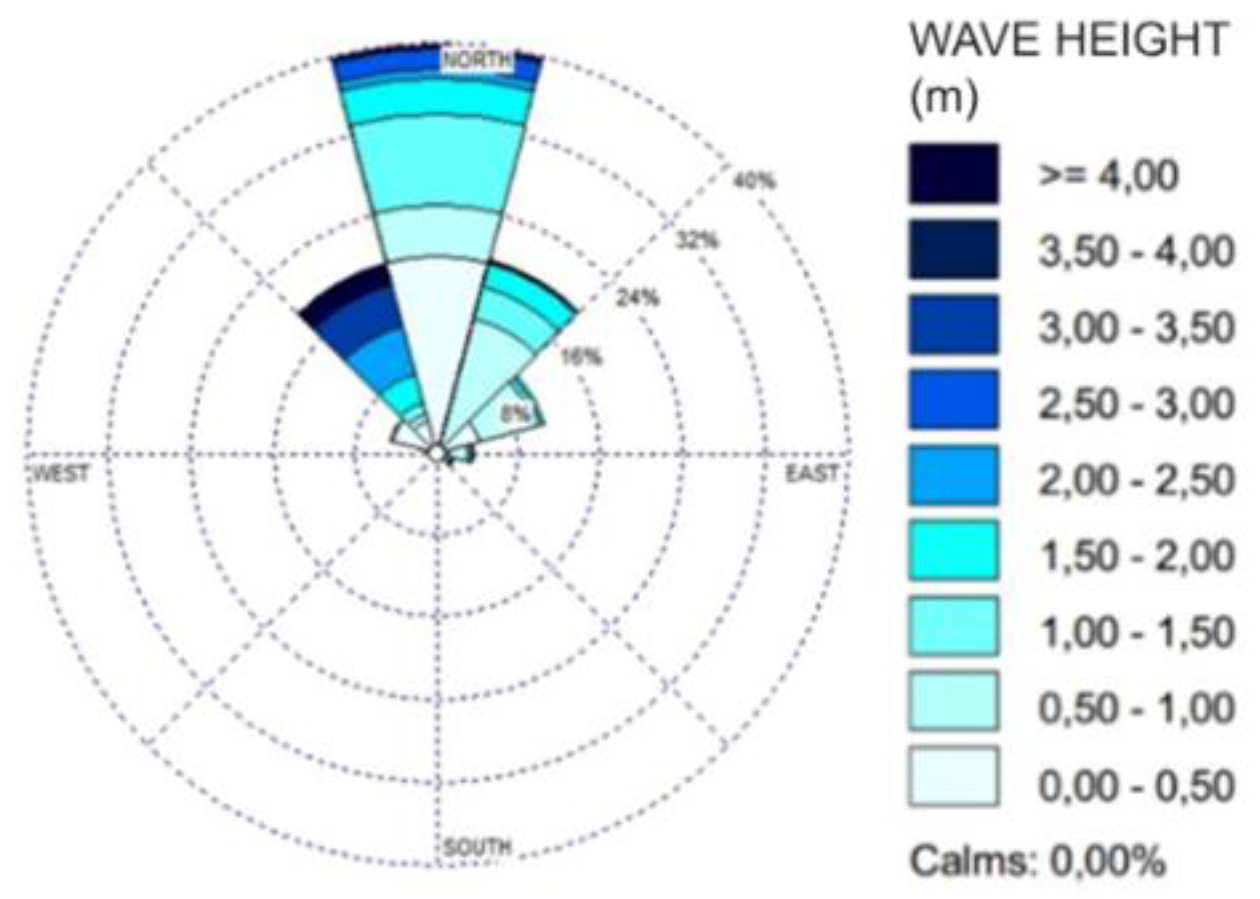
Figure 10.
Waverose Chart from 2019 to 2023 (Sverdrup Munk Bretschneider, Fully Developed).
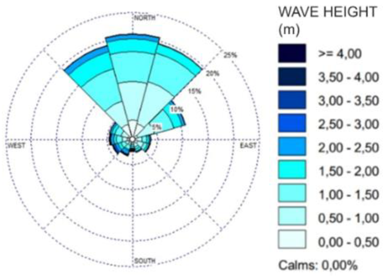

Table 1.
Wind Direction and Speed Table from 2019 to 2023.
| Month | 2019 | 2020 | 2021 | 2022 | 2023 | |||||
|---|---|---|---|---|---|---|---|---|---|---|
| Dir. (°) | Speed (m/s) | Dir. (°) | Speed (m/s) | Dir. (°) | Speed (m/s) | Dir. (°) | Speed (m/s) | Dir. (°) | Speed (m/s) | |
| January | 237 | 6 | 286 | 6 | 173 | 5 | 215 | 6 | 229 | 6 |
| February | 223 | 6 | 213 | 6 | 290 | 6 | 223 | 6 | 237 | 5 |
| March | 271 | 7 | 272 | 6 | 201 | 6 | 207 | 7 | 195 | 6 |
| April | 232 | 6 | 179 | 6 | 133 | 6 | 278 | 6 | 223 | 6 |
| May | 227 | 6 | 170 | 5 | 142 | 6 | 140 | 5 | 148 | 6 |
| June | 141 | 6 | 130 | 6 | 177 | 5 | 130 | 5 | 112 | 6 |
| July | 138 | 5 | 125 | 6 | 116 | 6 | 143 | 6 | 112 | 6 |
| August | 129 | 6 | 102 | 6 | 130 | 5 | 138 | 6 | 175 | 6 |
| September | 170 | 6 | 127 | 5 | 133 | 6 | 141 | 6 | 150 | 6 |
| October | 172 | 5 | 135 | 5 | 167 | 6 | 154 | 5 | 213 | 5 |
| November | 210 | 5 | 206 | 5 | 258 | 6 | 241 | 5 | 286 | 5 |
| December | 291 | 5 | 299 | 5 | 310 | 6 | 222 | 5 | 255 | 5 |
Table 2.
Table of Fetch Length on Cermin Beach.
| α | Fetch Length (km) |
|---|---|
| 120 | 456,93 |
| 114 | 292,66 |
| 108 | 257,73 |
| 102 | 261,31 |
| 96 | 238,35 |
| 90 | 223,13 |
| 84 | 198,4 |
| 78 | 195,63 |
| 72 | 191,24 |
| 66 | 194,21 |
| 60 | 205,1 |
| 54 | 216,41 |
| 48 | 214,85 |
| 42 | 227,14 |
| 36 | 222,21 |
| 30 | 296,43 |
| 24 | 316,48 |
| 18 | 296,39 |
| 12 | 324,52 |
| 6 | 317 |
| 0 | 455,65 |
| -6 | 470,54 |
| -12 | 587,69 |
| -18 | 1000 |
| -24 | 1000 |
| -30 | 1000 |
| -36 | 1000 |
| -42 | 115,33 |
Table 3.
Table of Wave Height and Period from 2019 to 2023 (Jonswap Parameters).
| Month | 2019 | 2020 | 2021 | 2022 | 2023 | |||||
|---|---|---|---|---|---|---|---|---|---|---|
| Height (m) | Period (s) | Height (m) | Period (s) | Height (m) | Period (s) | Height (m) | Period (s) | Height (m) | Period (s) | |
| January | 0,687 | 8,981 | 0,646 | 8,801 | 0,586 | 8,513 | 0,642 | 8,785 | 0,653 | 8,802 |
| February | 0,686 | 8,995 | 0,662 | 8,895 | 0,707 | 9,075 | 0,703 | 9,064 | 0,632 | 8,754 |
| March | 0,754 | 9,279 | 0,735 | 9,195 | 0,720 | 9,129 | 0,765 | 9,317 | 0,691 | 9,004 |
| April | 0,690 | 8,988 | 0,648 | 8,824 | 0,656 | 8,846 | 0,725 | 9,049 | 0,698 | 9,051 |
| May | 0,668 | 8,819 | 0,627 | 8,717 | 0,706 | 9,051 | 0,631 | 8,713 | 0,728 | 9,118 |
| June | 0,660 | 8,828 | 0,644 | 8,768 | 0,633 | 8,741 | 0,594 | 8,576 | 0,660 | 8,871 |
| July | 0,597 | 8,570 | 0,679 | 8,925 | 0,672 | 8,899 | 0,661 | 8,890 | 0,638 | 8,766 |
| August | 0,638 | 8,745 | 0,646 | 8,807 | 0,594 | 8,544 | 0,683 | 8,947 | 0,646 | 8,802 |
| September | 0,702 | 8,939 | 0,606 | 8,571 | 0,717 | 9,054 | 0,656 | 8,844 | 0,656 | 8,844 |
| October | 0,582 | 8,478 | 0,594 | 8,543 | 0,679 | 8,948 | 0,631 | 8,706 | 0,582 | 8,488 |
| November | 0,582 | 8,510 | 0,629 | 8,711 | 0,683 | 8,943 | 0,609 | 8,640 | 0,625 | 8,692 |
| December | 0,594 | 8,558 | 0,601 | 8,590 | 0,661 | 8,880 | 0,582 | 8,484 | 0,605 | 8,630 |
Table 4.
Table of Wave Height and Period from 2019 to 2023 (Finite Water Depth, 3 meter).
| Month | 2019 | 2020 | 2021 | 2022 | 2023 | |||||
|---|---|---|---|---|---|---|---|---|---|---|
| Height (m) | Period (s) | Height (m) | Period (s) | Height (m) | Period (s) | Height (m) | Period (s) | Height (m) | Period (s) | |
| January | 1,133 | 4,374 | 1,253 | 4,680 | 1,546 | 5,406 | 1,264 | 4,702 | 1,316 | 4,825 |
| February | 1,087 | 4,288 | 1,162 | 4,508 | 1,040 | 4,114 | 1,033 | 4,150 | 1,300 | 4,869 |
| March | 0,872 | 3,631 | 0,950 | 3,878 | 0,986 | 3,913 | 0,853 | 3,610 | 1,086 | 4,230 |
| April | 1,130 | 4,321 | 1,222 | 4,634 | 1,229 | 4,633 | 1,157 | 4,448 | 1,032 | 4,133 |
| May | 1,346 | 4,743 | 1,345 | 4,947 | 1,091 | 4,221 | 1,389 | 5,083 | 1,049 | 4,163 |
| June | 1,324 | 4,839 | 1,360 | 4,955 | 1,323 | 4,914 | 1,454 | 5,276 | 1,191 | 4,568 |
| July | 1,483 | 5,263 | 1,199 | 4,549 | 1,226 | 4,610 | 1,167 | 4,558 | 1,318 | 4,896 |
| August | 1,357 | 4,932 | 1,255 | 4,735 | 1,511 | 5,339 | 1,185 | 4,542 | 1,267 | 4,732 |
| September | 1,310 | 4,591 | 1,493 | 5,247 | 1,156 | 4,311 | 1,249 | 4,700 | 1,246 | 4,681 |
| October | 1,594 | 5,468 | 1,466 | 5,212 | 1,155 | 4,454 | 1,362 | 4,880 | 1,567 | 5,434 |
| November | 1,540 | 5,459 | 1,359 | 4,942 | 1,179 | 4,418 | 1,391 | 5,059 | 1,377 | 4,972 |
| December | 1,484 | 5,275 | 1,456 | 5,191 | 1,188 | 4,546 | 1,548 | 5,405 | 1,409 | 5,168 |
Table 5.
Table of Wave Height and Period from 2019 to 2023 (Finite Water Depth, 10 meter).
| Month | 2019 | 2020 | 2021 | 2022 | 2023 | |||||
|---|---|---|---|---|---|---|---|---|---|---|
| Height (m) | Period (s) | Height (m) | Period (s) | Height (m) | Period (s) | Height (m) | Period (s) | Height (m) | Period (s) | |
| January | 2,192 | 6,978 | 2,340 | 7,202 | 2,501 | 7,318 | 2,354 | 7,230 | 2,339 | 7,081 |
| February | 2,218 | 7,077 | 2,322 | 7,208 | 2,110 | 6,931 | 2,183 | 7,007 | 2,419 | 7,283 |
| March | 1,930 | 6,722 | 2,025 | 6,778 | 2,042 | 6,887 | 1,959 | 6,709 | 2,174 | 7,023 |
| April | 2,154 | 6,930 | 2,356 | 7,250 | 2,308 | 7,138 | 2,251 | 6,951 | 2,174 | 7,050 |
| May | 2,219 | 6,851 | 2,410 | 7,241 | 2,116 | 6,879 | 2,451 | 7,200 | 2,175 | 6,922 |
| June | 2,283 | 6,951 | 2,338 | 7,042 | 2,421 | 7,231 | 2,554 | 7,408 | 2,328 | 7,171 |
| July | 2,486 | 7,312 | 2,272 | 7,004 | 2,267 | 7,023 | 2,351 | 7,211 | 2,385 | 7,179 |
| August | 2,363 | 7,124 | 2,360 | 7,196 | 2,516 | 7,298 | 2,274 | 6,995 | 2,341 | 7,181 |
| September | 2,089 | 6,586 | 2,458 | 7,217 | 2,094 | 6,703 | 2,304 | 7,103 | 2,309 | 7,121 |
| October | 2,484 | 7,264 | 2,494 | 7,340 | 2,260 | 7,052 | 2,347 | 7,142 | 2,510 | 7,313 |
| November | 2,559 | 7,375 | 2,390 | 7,191 | 2,186 | 6,971 | 2,479 | 7,353 | 2,381 | 7,198 |
| December | 2,507 | 7,356 | 2,475 | 7,326 | 2,303 | 7,179 | 2,508 | 7,322 | 2,521 | 7,388 |
Table 6.
Table of Wave Height and Period from 2019 to 2023 (Sverdrup Munk Bretschneider, Fetch Limited).
Table 6.
Table of Wave Height and Period from 2019 to 2023 (Sverdrup Munk Bretschneider, Fetch Limited).
| Month | 2019 | 2020 | 2021 | 2022 | 2023 | |||||
|---|---|---|---|---|---|---|---|---|---|---|
| Height (m) | Period (s) | Height (m) | Period (s) | Height (m) | Period (s) | Height (m) | Period (s) | Height (m) | Period (s) | |
| January | 1,327 | 2,837 | 1,527 | 3,745 | 1,858 | 4,985 | 1,543 | 3,814 | 1,561 | 3,801 |
| February | 1,268 | 2,576 | 1,341 | 2,805 | 1,237 | 2,540 | 1,206 | 2,355 | 1,488 | 3,326 |
| March | 1,071 | 2,013 | 1,134 | 2,174 | 1,237 | 2,718 | 1,032 | 1,828 | 1,320 | 2,934 |
| April | 1,374 | 3,166 | 1,452 | 3,340 | 1,462 | 3,405 | 1,332 | 2,830 | 1,215 | 2,404 |
| May | 1,746 | 4,967 | 1,583 | 3,815 | 1,296 | 2,787 | 1,581 | 3,682 | 1,224 | 2,454 |
| June | 1,537 | 3,632 | 1,571 | 3,724 | 1,546 | 3,654 | 1,683 | 4,113 | 1,407 | 3,160 |
| July | 1,781 | 4,678 | 1,421 | 3,261 | 1,426 | 3,196 | 1,328 | 2,705 | 1,511 | 3,439 |
| August | 1,609 | 3,976 | 1,476 | 3,404 | 1,836 | 4,961 | 1,361 | 2,912 | 1,502 | 3,543 |
| September | 1,692 | 4,770 | 1,985 | 6,458 | 1,417 | 3,424 | 1,444 | 3,223 | 1,446 | 3,247 |
| October | 1,965 | 5,545 | 1,972 | 6,420 | 1,342 | 2,858 | 1,738 | 4,805 | 1,922 | 5,342 |
| November | 1,790 | 4,553 | 1,646 | 4,200 | 1,441 | 3,448 | 1,673 | 4,249 | 1,674 | 4,323 |
| December | 1,781 | 4,665 | 1,755 | 4,590 | 1,382 | 2,993 | 2,036 | 6,580 | 1,599 | 3,703 |
Table 7.
Table of Wave Height and Period from 2019 to 2023 (Sverdrup Munk Bretschneider, Fully Developed).
Table 7.
Table of Wave Height and Period from 2019 to 2023 (Sverdrup Munk Bretschneider, Fully Developed).
| Month | 2019 | 2020 | 2021 | 2022 | 2023 | |||||
|---|---|---|---|---|---|---|---|---|---|---|
| Height (m) | Period (s) | Height (m) | Period (s) | Height (m) | Period (s) | Height (m) | Period (s) | Height (m) | Period (s) | |
| January | 1,092 | 5,036 | 0,924 | 4,664 | 0,744 | 4,145 | 0,909 | 4,630 | 1,053 | 4,759 |
| February | 1,054 | 5,016 | 0,959 | 4,800 | 1,150 | 5,209 | 1,132 | 5,168 | 0,863 | 4,537 |
| March | 1,335 | 5,636 | 1,276 | 5,471 | 1,205 | 5,335 | 1,439 | 5,750 | 1,086 | 5,063 |
| April | 1,116 | 5,073 | 0,913 | 4,676 | 0,966 | 4,754 | 1,857 | 5,492 | 1,093 | 5,122 |
| May | 1,191 | 4,925 | 0,865 | 4,499 | 1,192 | 5,212 | 0,959 | 4,553 | 1,494 | 5,453 |
| June | 1,066 | 4,817 | 0,987 | 4,671 | 0,894 | 4,550 | 0,733 | 4,199 | 0,969 | 4,783 |
| July | 0,774 | 4,241 | 1,142 | 4,989 | 1,087 | 4,916 | 0,956 | 4,785 | 0,916 | 4,602 |
| August | 0,958 | 4,616 | 0,922 | 4,662 | 0,784 | 4,215 | 1,152 | 5,020 | 0,928 | 4,665 |
| September | 1,393 | 5,253 | 0,880 | 4,341 | 1,366 | 5,359 | 0,974 | 4,756 | 0,974 | 4,756 |
| October | 0,758 | 4,123 | 0,763 | 4,211 | 1,074 | 4,970 | 0,915 | 4,549 | 0,742 | 4,117 |
| November | 0,716 | 4,105 | 0,893 | 4,522 | 1,114 | 5,012 | 0,792 | 4,339 | 0,876 | 4,488 |
| December | 0,752 | 4,204 | 0,779 | 4,271 | 0,964 | 4,790 | 0,740 | 4,118 | 0,764 | 4,291 |
Table 8.
Return Period with Weibull Distribution (Jonswap Parameters).
| Return Period (Year) | |||||||
|---|---|---|---|---|---|---|---|
| Ht | λ | α | β | ϒ | 20 | 50 | 100 |
| 0,5 | 209,75 | 1,3 | 0,358 | 0,541 | 2,838 | 3,091 | 3,282 |
| 1 | 51 | 1 | 0,387 | 0,837 | 3,521 | 3,876 | 4,144 |
| 1,5 | 5,75 | 1,1 | 0,670 | 0,956 | 3,845 | 4,403 | 4,825 |
Table 9.
Return Period with Gumbel Distribution (Finite Water Depth, 3 Meter).
| Return Period (Year) | ||||||
|---|---|---|---|---|---|---|
| Ht | λ | β | ϒ | 20 | 50 | 100 |
| 0,5 | 300 | 0,408 | 1,037 | 4,587 | 4,961 | 5,244 |
| 1 | 195,5 | 0,271 | 1,419 | 3,661 | 3,909 | 4,097 |
| 1,5 | 77 | 0,195 | 1,893 | 3,327 | 3,506 | 3,641 |
Table 10.
Return Period with Gumbel Distribution (Finite Water Depth, 10 Meter).
| Return Period (Year) | ||||||
|---|---|---|---|---|---|---|
| Ht | λ | β | ϒ | 20 | 50 | 100 |
| 0,5 | 343,5 | 0,818 | 1,904 | 9,129 | 9,878 | 10,445 |
| 1 | 318,5 | 0,512 | 1,979 | 6,462 | 6,931 | 7,286 |
| 1,5 | 285,75 | 0,390 | 2,142 | 5,519 | 5,876 | 6,147 |
Table 11.
Return Period with Weibull Distribution (Sverdrup Munk Bretschneider, Fetch Limited).
| Return Period (Year) | |||||||
|---|---|---|---|---|---|---|---|
| Ht | λ | α | β | ϒ | 20 | 50 | 100 |
| 0,5 | 247,75 | 1,3 | 0,747 | 0,689 | 5,581 | 6,108 | 6,507 |
| 1 | 125,5 | 1 | 0,700 | 1,189 | 6,672 | 7,313 | 7,799 |
| 1,5 | 72,75 | 1,1 | 0,676 | 1,514 | 5,987 | 6,550 | 6,976 |
Table 12.
Return Period with Weibull Distribution (Sverdrup Munk Bretschneider, Fully Developed).
| Return Period (Year) | |||||||
|---|---|---|---|---|---|---|---|
| Ht | λ | α | β | ϒ | 20 | 50 | 100 |
| 0,5 | 365,25 | 1,3 | 0,574 | 0,622 | 4,551 | 4,956 | 5,262 |
| 1 | 221,75 | 1 | 0,668 | 0,688 | 6,301 | 6,913 | 7,377 |
| 1,5 | 31,25 | 1,1 | 0,624 | 1,750 | 5,400 | 5,919 | 6,312 |
Disclaimer/Publisher’s Note: The statements, opinions and data contained in all publications are solely those of the individual author(s) and contributor(s) and not of MDPI and/or the editor(s). MDPI and/or the editor(s) disclaim responsibility for any injury to people or property resulting from any ideas, methods, instructions or products referred to in the content. |
© 2025 by the authors. Licensee MDPI, Basel, Switzerland. This article is an open access article distributed under the terms and conditions of the Creative Commons Attribution (CC BY) license (http://creativecommons.org/licenses/by/4.0/).
Copyright: This open access article is published under a Creative Commons CC BY 4.0 license, which permit the free download, distribution, and reuse, provided that the author and preprint are cited in any reuse.