
Submitted:
13 July 2025
Posted:
14 July 2025
You are already at the latest version
Abstract
In many practical applications, data collected over time exhibit auto-correlation, which, if not addressed, can lead to incorrect statistical inferences. To address this, we propose a varying-coefficient additive model with density responses, incorporating a functional autoregressive (FAR) error process to account for serial dependency. We present a three-step spline-based estimation procedure for the varying-coefficient components after mapping densities into a linear space using the log-quantile density transformation. First, a B-spline series approximation provides initial estimates of the bivariate varying-coefficient functions. Second, spline estimation of the error process is obtained from the residuals. Lastly, improved estimates of the additive components are obtained by removing the estimated error process. Theoretical results, including convergence rates and asymptotic properties, are provided, and the practical performance of the method is demonstrated through simulations and real data analyses.
Keywords:
varying-coefficient
; density response
; functional auto-regressive error process
; log quantile density transformation
1. Introduction
Density, or more generally, distributional data appear increasingly often in various real-world research domains. Specific examples include the distributions of cross-sectional or intraday stock returns [9,15], mortality densities [13], and distributions of intrahub connectivity in neuroimaging [11,14]. In many applications, the density curves are observed consecutively over time, which we call in the article a density time series. A motivating example is shown in Figure 1, (a) shows density time series of global mortality rate (‰) over an interval of 100 days from January 22, 2020 to April 15, 2021, while Figure (b) is an alternative look with plotting densities at three different days. In this article, we consider a regression model where density time series, served as response, is coupled with scalar predictors.
Unlike conventional functional data, density data do not form a linear space due to inherent constraints, such as nonnegativity and the requirement to integrate to one. These characteristics present significant challenges when attempting to directly apply functional data analysis techniques to random densities. Several studies have addressed this issue and proposed various solution methods, which can be broadly categorized into two types. One natural approach to overcoming the nonlinear limitations of density functions is to map them into a Hilbert space using a suitable transformation method. In this direction, [12] proposed two continuous and invertible transformations, which are log hazard transformation and log quantile density (LQD) transformation, to map probability densities to an unrestricted space of square integrable functions. [8] map densities by LQD transformation as in [12] to unrestricted square integrable functions, model and fit the responses with an additive functional-to-scalar regression. In order to forecast density functions derived from cross-sectional and intraday returns, [9] proposed two approaches based on compositional data analysis and modified log quantile transformation, combining the FPC representation and exponential smoothing forecasting method. The second way involves choosing appropriate metrics and adopting a geometric approach. For instance, [17] adopted the infinite-dimension version of the Aitchison geometry to construct a density-on-scalar linear regression model in Bayes–Hilbert spaces, while [13] discussed Fréchet regression in a general metric space with the Wasserstein metric. [5] utilized the geometry of tangent bundles of the Wasserstein space with the Wasserstein metric to propose distribution-on-distribution regression. They also studied an extension to autoregressive models of order one for distribution-valued time series. With different methodology, [19] also discussed order-p Wasserstein autoregressive model.
Denote as the space of density functions f defined on a common support . Without of generality, we assume that . Given the transformation , for any given , the conditional Fréchet mean of the random density f is defined as
where the expectation E represents the joint distribution of .
This is equivalent to the following equation
leading to the fact that
Data that we consider in this article are the density time series coupled with scalar predictors . To deal with the density functions, we adopt the LQD transformation , where is the class of density function d satisfying . For each , let be the quantile function corresponding to the cumulative distribution function of with support on [0,1], and be the quantile density function, i.e., for , then the LQD transformation of is defined as
In this article, a varying-coefficient additive model with functional auto-regressive error process is proposed to estimate . Then can be written as
where is the error from regression.
Except for , there is usually another source of error, which comes from the estimation of , i.e., . That is because in most practical applications, instead of the density itself, only random samples generated from each can be observed. Namely, . In this article, we assume that . Following [12], is estimated by the modified kernel smoothing method, i.e,
where the weight function is defined so as to rectify the boundary effects as follows:
in which is the kernel with bandwidth and bounded variation that is symmetric about 0 such that , , , and are finite. Thus, when we fit the regression model with as the observation of , we have
The contribution of this article lies in integrating density time series modeling with a functional autoregressive error process. A common assumption in regression modeling is the independence of random errors. However, data collected over time often exhibit serial dependence, rendering this assumption potentially inappropriate. By incorporating autoregressive structures into the error process, this work accounts for the temporal correlation inherent in density time series, thereby improving the model’s flexibility and accuracy. For example, daily price curves or liquidity demand-supply curves in economic and financial applications or climatological curves describing the natural phenomenon [1,3,4,6] all change over time. In such cases, the daily fluctuations in the collected data are heavily influenced by previous values, potentially resulting in what is known as sequence dependence. Numerous empirical studies have demonstrated that neglecting the temporal dependencies between observations can lead to biased statistical results and flawed inferences. Consequently, it is crucial to incorporate autoregressive error structures that explicitly account for the autocorrelation present within the data. This approach ensures a more accurate representation of the underlying temporal dynamics in regression modeling. While functional autoregressive (FAR) models have been extensively studied in the literature [1,2,3,4,6,10,18], there is a notable gap in the literature regarding the use of FAR processes to model the random error component in functional regression models. In this article, to improve the accuracy of density time series predictions, we integrate the FAR error structure within a varying coefficient additive regression model. This novel approach allows for better handling of temporal dependencies in the error process, ultimately enhancing the model’s predictive performance.
The remainder of this article is organized as follows. Section 2 outlines the methodology for constructing a varying coefficient additive model with a density response, incorporating a functional autoregressive (FAR) error process. In Section 3, we introduce a three-step procedure for estimating the bivariate varying-coefficient components within the model. Section 4 provides the theoretical results and corresponding inferences derived from the model. Monte Carlo simulations are conducted in Section 5 to demonstrate the efficiency and robustness of the proposed approach. In Section 6, we showcase the practical applicability of the model through analyses of COVID-19 data and U.S. income data. Finally, a discussion of the findings is provided in Section 7, with detailed proofs of the theoretical results included in the Appendix.
2. Model Setup
In this article, we focus on the modeling of density response. Due to the constraints of density function which is nonnegative and integrated to 1, we consider the functions after LQD transformation.
In the article, the main goal is to estimate based on the transfer of density function as
leading to our proposed varying-coefficient additive models with density responses and functional auto-regressive error process (DVCA-FAR):
where is the process
In the above model, the random density serves as a response, and is the LQD transformation. Each density is coupled with the dimensional covariates and with supports and respectively. Without loss of generality, we take . In this article, covariate can be or .
The bivariate functions quantify the effect of , are smooth functions satisfying . Moreover, the error is an independent and identically distributed random process satisfying and .
With the estimated density , let . Then DVCA-FAR model can be written as
where is random error generated from the transformation of estimated density.
3. Three-Step Estimation Methodology
We propose a three-step estimation procedure. First, the B-spline smoothing method is employed to obtain the initial estimate of the bivariate varying coefficients, disregarding the error structure. Second, using the initial estimate and the response, we estimate the error process. The functional autoregressive (FAR) process is then estimated using the sequential test proposed by [10]. Finally, after removing the estimated FAR error, the optimal estimate is derived using the spline method.
3.1. Initial Estimation of Bivariate Varying-Coefficient Function
First, without considering error structure, we adopt the spline method to obtain the initial estimations of , regardless of the error process, by the spline series approximation method.
Let be the set of B-spline basis functions for u of order q with interior knots, where . Similarly, for each , let be the set of B-spline basis functions of order q for () with interior knots, where . Denote as the normalization of and as the scaled version of .
Using these basis functions, we define the tensor product of the B-spline basis as
The spline approximation of is given by
With the least square method, the estimation of is
where is a -dimensional vector satisfying
Theorem 1 shows that the initial estimation is uniformly consistent.
3.2. Estimation of FAR Error Process
With the initial estimation , we now estimate the FAR error process. To this end, let
Denote the additive function , thus the error process (3) can be written as .
Let be the set of B-spline basis functions of order q with L interior knots, where . Define the tensor product of the B-spline basis as
Then, the spline approximations of the functions is given by
The estimation of the -dimensional vector can be obtained by minimizing the following quadratic loss function:
Then, the corresponding estimation of and the additive function are given by
and
respectively.
In practice, the order p of error process is unknown. To solve this problem, we utilize a sequential test by [10] to identify the order p. The detailed identification procedure is given in Section 3.4.2.
3.3. Improved Estimation of Bivariate Varying-Coefficient Function
By removing the estimated error process (8) from the response function and repeating the same procedure as in Section 3.1, we obtain an improved estimation of .
To do so, we first denote
and the estimation of as
On the other side,
Therefore, following the same procedure as the first step, the improved spline approximation estimations are given by
where is a -dimensional vector satisfying
Theorem 2 and 3 show the uniform convergence and asymptotic normality of the improved estimation . Besides, simulation studies in Section 5 show that the improved estimation is more efficient than the initial estimation .
3.4. Implementation
3.4.1. Selection of Bandwidth
In empirical applications, prior to modeling, it is necessary to estimate the density, which involves selecting the appropriate bandwidth for the modified kernel estimation. In this section, we employ the leave-one-out cross-validation method to determine the optimal bandwidth. Specifically, the bandwidth h is chosen by minimizing the following mean squared error (MSE):
where for each , is the estimate of with bandwidth h obtained by using observations from the t-th section other than the i-th one.
3.4.2. Identifying the Order of the FAR Process
In this section, we utilize the order determination procedure proposed by [10] to identify th order p of FAR error process. The main idea is to represent the FAR process as a fully functional linear model with dependent regressors and construct a sequential test procedure.
Given a sequence of hypotheses:
Here, means independent and identically distributed process.The sequential test begins with and terminated if is not rejected, the order of the process is then identified as p. See [10] for more relevant details and further explanation.
To construct the test statistic, define where as the indicator function of the interval . Denote the orthonormal basis of as from the eigenfunctions of with the corresponding decreasingly ordered eigenvalues , where is the mean function of . In the proposed method, only the first eigenfunction/eigenvalue pairs are used. Moreover, define and analogously to and for the response functions denoted as .
For the product space , denote , , . Let , and , ; ; .
Construct the matrix in which the entries are where Define the orthonormal eigenvectors with corresponding ordered eigenvalues as and denote , where and .
Following [10], the test statistic is constructed as
where . The test statistic has an approximately chi-squared distribution with degree .
4. Theoretical Results
In this section, we discuss the asymptotic properties of both initial and improved estimation of . Moreover, the consistency of estimation of order p is derived. All proofs are given in Appendix.
Throughout the remainder of this article, for any fixed interval , we denote the space of l-th order smooth functions as and the class of Lipschitz-continuous functions for some fixed constant as Let and denote the supports of and , respectively. Then, the supports of and are and , respectively. The necessary assumptions for the asymptotic results are as follows.
(A1) For any , d is differentiable and there exists a constant such that , , and are all bounded by M.
(A2) (a) The kernel density is Lipschitz-continuous, bounded, and symmetric about 0. Furthermore, for some constant . (b) The kernel density is such that , , , and are finite.
(A3) The covariates , , and the errors satisfy the following moment conditions: for some ,
For each , the covariance function has finite nondecreasing eigenvalues satisfying .
(A4) The additive component functions , are continuous on and twice continuously partially differentiable with respect to u and , where is a compact subset of .
(A5) , , , , as .
Remark 1.
Assumption (A1) is basic and essential for deriving the consistency of densities after transformation. The conditions in (A2) on the kernel function are mild and can be satisfied by commonly used kernel functions such as the uniform and Epanechnikov kernels. The moment conditions in (A3) are crucial for deriving the uniform convergence and other asymptotic properties based on the spline function. The smoothness conditions for the component functions in (A4) are greatly relaxed. The conditions in (A5) are commonly applied in spline smoothing to ensure optimal convergence rates.
We first derive the uniform consistency of the initial estimates of bivariate functions , as stated in Theorem 1.
Theorem 1.
Theorem 1. Assume that assumptions (A1)–(A5) hold, and that are the initial estimates of defined by (5), . Then, as and , it holds that
Theorem 2 characterizes the uniform convergence of the improved estimation of , and Theorem 3 describes the asymptotic properties of both the initial and improved estimations.
Theorem 2.
Theorem 2.Assume that assumptions (A1)–(A5) hold, are the improved estimates of defined by (9), , and that the order of the functional error process p is known. Then, as and , the following holds:
To present the asymptotic normality of the estimations, some notations are given as follows. Denote , , , , and .
Let , and is an block matrix, with the m-th block being identity matrix and the j-th () block being zero matrix.
Theorem 3.
Theorem 3.Assume that assumptions (A1)–(A5) hold, and are the initial and improved estimates of defined by (5) and (9), , respectively. Then, as , the following hold for all and :
(i) The initial estimate is asymptotically normally distributed, i.e.,
where , the covariance matrix , with .
(ii) The improved estimate is asymptotically normally distributed, i.e.,
where the covariance matrix , with .
5. Numerical Study
In this section, we conduct two simulation studies to demonstrate the performance of the proposed identification and estimation procedure for the additive model.
5.1. Case 1
With the assumption that the auto-regressive error process is known, this case is conducted to demonstrate the performance of the estimation procedure with finite n and T. We consider the following DVCA-FAR(1) model:
and the error function is
Let the bivariate varying-coefficient functions be
and the coefficient functions be
where , , and are independent of for .
The covariates are generated by and , respectively, while are generated by , , where is the cumulative distribution function of the standard normal distribution and , are mutually independent variables of the standard normal distribution.
To generate the response densities, for each given and , let be the additive surface given by . The conditional quantile function with the error process satisfy , where .
Implementing the conditional quantile function to , which are independent of and , we can get the random samples for each , so that , where is the random response density. Denoting , we obtain the transformed density expressed in model (2). Without loss of generality, we assume that independent and identically distributed observations are available for each response distribution.
With , the estimation is conducted with 200 Monte Carlo runs. Figure 2 displays the true curves of the FAR error process in panel (a) and its corresponding spline-based estimations in panel (b). Figure 3 presents a comprehensive view of the true surface of alongside the average estimations obtained from 200 Monte Carlo simulations. Specifically, the left panel displays the true densities, the middle panel shows the initial spline estimates derived without accounting for the error process, and the right panel provides the improved estimations achieved through the same method after removing the estimated error process. To better illustrate the performance, the bivariate function estimations are presented from two different relative perspectives, offering a clearer understanding of the improvements made through the error correction process.
Figure 2 indicates that the estimation of yields highly accurate results, which is further corroborated by the findings presented in Figure 3. Specifically, the right panel of Figure 3 illustrates that the improved estimation, after accounting for the FAR error process, significantly outperforms the initial estimation shown in the middle panel. This improvement highlights the effectiveness of the proposed methodology in refining the bivariate function estimates by appropriately addressing the error structure.
For further comparison, we conducted simulations with sample sizes of and observations. We use the root mean squared errors (RMSEs) to measure the accuracy of the estimations, including the initial and improved estimations of . The RMSE is defined as
where is or .
Based on the results from 200 Monte Carlo simulations, Table 1 presents the average root mean square errors (RMSEs) along with their standard deviations for both the initial and improved estimations of . The findings reveal that the RMSEs of the bivariate functions decrease as both the sample size T and the number of observations n increase. Notably, the RMSEs associated with the improved estimation are consistently smaller than those for the initial estimation. This is to be expected, as the initial estimates were derived without accounting for the error process, which, as demonstrated, has a significant impact on the accuracy of the results. By incorporating the error process and removing its estimated effects in the improved estimation, the model yields more accurate and refined results.
To provide a clearer explanation of the theoretical validity differences between the two estimations, we calculate their biases and standard deviations and compare them. Taking the first example in the numerical simulation section as an example.
Table 2 presents the average bias and standard deviation (SD) of both the initial and improved estimations of . The results clearly indicate that, across all settings of the model sample size, the standard deviation of the improved estimates of the bivariate additive functions is substantially smaller than that of the initial estimates, with the bias also being correspondingly reduced. Moreover, as the sample size increases, both the standard deviation and bias of the estimates decrease, further reinforcing the reliability of the improved method. This finding numerically substantiates the claim that the improved estimation method results in a smaller asymptotic variance-covariance matrix compared to the initial estimation, thereby enhancing the precision and robustness of the estimates.
5.2. Case 2
Case 2 is conducted to demonstrate the efficiency of identifying the auto-regressive order of the functional error process. The densities are also generated from model (12), but with the error function, where . All other settings are the same as for Case 1.
Table 3 presents the empirical power of the testing algorithm used to determine the order of the FAR error process under various settings and significance levels. The results clearly demonstrate that the power of the test increases as the sample size T and the number of observations n grow. Specifically, the power approaches 1 as both T and n increase to 100 when testing the null hypothesis of an independent and identically distributed (i.i.d.) sample. This suggests that the test becomes increasingly reliable with larger sample sizes. However, the power is slightly lower when testing the null hypothesis of order 1 against order 2, which is expected given the complexity of distinguishing between these two orders. Furthermore, the size of the test remains low when testing order 2 against a higher-order process, confirming the accuracy and feasibility of the testing algorithm for determining the appropriate order of the functional error process. These findings validate the effectiveness of the proposed testing algorithm in practical applications, ensuring its robustness and precision in various settings.
Furthermore, to assess the efficiency of the auto-regressive order p on the overall estimation results, Table 4 presents the average RMSEs for the bivariate varying-coefficient functions. The observed pattern closely mirrors the results from Case 1, further reinforcing the effectiveness and reliability of the proposed model’s identification and estimation procedures. These findings provide strong empirical evidence that the auto-regressive order plays a crucial role in enhancing the accuracy of the estimation process. The consistency of the RMSE results across different settings underscores the robustness of the model, confirming its ability to effectively account for the error structure and yield precise estimates of the bivariate varying-coefficient functions.
6. Real Data Analysis
In this section, we demonstrate the feasibility and efficiency of the proposed estimation procedure through the analysis of two real-world datasets. By applying the developed methodology to empirical data, we aim to showcase the practical utility of the model in capturing the underlying patterns and dependencies inherent in the datasets. The analysis serves not only to validate the effectiveness of the proposed estimation approach but also to highlight its applicability across different domains, offering insights into the model’s versatility and robustness in handling complex, time-dependent, and non-Euclidean data structures.
6.1. COVID-19 Data
On March 11, 2020, the World Health Organization (WHO) declared COVID-19, an infectious disease caused by the severe acute respiratory syndrome coronavirus 2 (SARS-CoV-2), a global pandemic. The rapid and widespread transmission of the virus led to unprecedented global health challenges, with countries around the world instituting lockdowns and other measures to curb the spread of the disease. As of August 15, 2021, official statistics from the WHO reported a staggering 221,885,822 confirmed cases and 4,583,539 deaths across nearly all countries, reflecting the profound and far-reaching impact of the pandemic. Given the magnitude of this crisis, it is essential for international health organizations and research institutions to closely monitor the evolving global trends of COVID-19. Such monitoring facilitates timely and accurate analysis, enabling effective public health responses and the development of strategies for medical treatment, prevention, and control of future outbreaks. Understanding the dynamics of the epidemic through data-driven models is thus critical for informing policy decisions and improving global health outcomes in the face of such a devastating crisis.
To demonstrate this proposition, we select the mortality rate as an appropriate metric for measuring the global trend of the COVID-19 pandemic. The mortality rate is defined as the ratio of cumulative deaths per day to the total population of each country, serving as a key indicator of the disease’s lethality and spread. Notably, the data required to calculate the mortality rate are inherently temporally dependent, as they rely on the data from the previous day. This results in the mortality rate, and thus the global trend of the epidemic, exhibiting temporal auto-correlation.
The data on COVID-19-related deaths, which are critical for our analysis, can be accessed from the Johns Hopkins University repository. This repository includes a dynamic tracking map that provides a comprehensive view of the global trends related to the pandemic. The dataset, which is publicly available at https://www.jhu.edu/, covers the period from January 22, 2020, to April 15, 2021. Additionally, the most recent total population data for each country, necessary for calculating the mortality rate, can be obtained from the World Bank’s online platform, accessible at https://data.worldbank.org/indicator. These publicly available datasets serve as a rich resource for tracking the progression of the pandemic and for conducting rigorous statistical and epidemiological analyses aimed at understanding the disease dynamics across different regions.
Due to the varying outbreak times across different countries and regions, we define the origin of the time scale as the point at which the cumulative number of confirmed COVID-19 cases reached 100 in all countries. For this analysis, we focus on a dataset containing daily cumulative deaths from 189 countries, considering a 100-day period following this reference time. At each time point t, we estimate the density function of the mortality rate, denoted as , using the observations from the 189 countries. Figure 1 (a) presents the estimated densities of the global mortality rate (‰) over the 100-day interval, with data records from up to 189 countries for each time point. Figure 1 (b) offers an alternative perspective by displaying the estimated densities for three selected days. From the figures, it is evident that the mortality rate densities are well-defined across the observed period. Moreover, a temporal dependency among the distributions is clearly observable, which suggests the presence of an auto-regressive process in the data, potentially supporting the hypothesis of a FAR error structure.
The primary goal of this analysis, based on the COVID-19 data, is to identify the FAR process underlying the mortality rate and estimate its component functions. For the sake of simplicity, we begin by considering a special case in which the covariate z is constant (=1) and x represents a time scale, denoted as , namely, we consider the following model:
where and denotes the time scale .
Based on the initial spline estimation of , the testing algorithm is employed to determine the order of the FAR process. Table 5 presents the test results, specifically the p-values under different hypotheses. The table reveals that the observed p-values indicate significant evidence of auto-correlation in the data. This suggests that the underlying process can indeed be effectively modeled as a first-order functional auto-regressive process, denoted as . Such findings provide strong empirical support for the presence of temporal dependencies in the COVID-19 mortality rate, further justifying the application of a FAR error structure in modeling the dynamics of the epidemic.
Figure 4 presents the heat map of the estimated bivariate function after accounting for the functional error process and identifying the auto-regressive order. The heat map reveals a relatively stable temporal pattern, with the function initially reaching a minimum value at lower values of u, gradually increasing, and eventually reaching a maximum at later time points. This pattern highlights the underlying dynamics of the COVID-19 mortality rate across successive days. The observed correlation between the data from consecutive days supports the notion that the global mortality rate exhibits significant temporal dependencies. This is consistent with the design of the mortality rate measure, which is derived from previous daily data, reflecting the evolving trend of the pandemic on a global scale. The results further validate the presence of auto-correlation in the mortality rate data and underscore the necessity of incorporating a functional auto-regressive process to capture these dependencies effectively.
6.2. USA Income Data
Personal income statistics play a crucial role in enabling governments to understand the dynamics between national income, spending, and saving, while also serving as an important tool for evaluating and comparing the economic well-being across different regions or nations. In this context, we focus on the density time series of per capita personal income, which is defined as the total personal income of an area divided by its population. This measure provides a more granular perspective on the economic conditions within a region, reflecting the distribution and trends in income on a per-person basis over time. By analyzing such time series, policymakers and researchers can gain insights into the long-term economic trajectory of a region, assess disparities in income distribution, and make informed decisions regarding fiscal policies, social welfare programs, and economic development strategies.
Income data for the USA are publicly available at the official website of the United States Bureau of Economic Analysis (http://www.bea.gov/). We consider the quarterly per capita personal income of 50 states in the USA from the first quarter of 2010 to the fourth quarter of 2020, namely, . For each t, we obtain the density function of per capita income, , each with 50 observations. As the quarterly personal income is an economic measure based on national conditions, we choose two related covariates, `GDP’ (quarterly gross domestic product of the USA) and `Population’ (quarterly total population of the USA), which can also be obtained from http://www.bea.gov/.
The income curve, traditionally studied in economics as panel data, primarily reflects the relationship between consumers’ equilibrium points. As individuals’ income levels fluctuate, the connections between these equilibrium points form a trajectory, symbolizing not only an increase in income but also a corresponding rise in consumer satisfaction. This approach emphasizes the dynamic nature of income growth and its impact on individual well-being, providing valuable insights into consumer behavior over time.
In contrast, the income density curve, treated as functional data, is used to describe the distribution of income within a specific region or demographic group. It offers a graphical representation of the characteristics and trends in income across various income intervals, providing a more holistic view of the socio-economic landscape. By analyzing the income density curve, the degree of income inequality within a population can be effectively observed, revealing important patterns of wealth distribution. This type of curve is crucial for economic research as it facilitates a deeper understanding of consumption behavior, socio-economic conditions, and the formulation of societal policies.
Moreover, income density curves are instrumental in economic forecasting and analysis. By examining trends in income distribution, economists can combine insights into consumer preferences and consumption habits at different income levels. This integration enables predictions about future economic conditions and shifts in consumption patterns, making the income density curve a key tool for anticipating changes in both microeconomic and macroeconomic contexts. In this way, the income density curve plays an essential role in informing policy decisions, economic strategies, and the broader understanding of economic well-being.
Figure 5 (a) illustrates the density time series of quarterly personal income over a period of 44 quarters. The density curves reveal that, over the past decade, the overall distribution of per capita income across various states in the United States has exhibited a consistent pattern. Specifically, there are relatively few individuals in the high-income and middle-to-high-income brackets, a moderate number in the middle-income category, and a larger proportion in the middle-to-low-income segments.
To further elucidate the temporal evolution of income distribution, Figure 5 (b) presents the density curves for three distinct time points: the second quarter of 2015, the first quarter of 2017, and the third quarter of 2018. A clear trend emerges, showing a gradual shift towards higher income values over time, accompanied by a corresponding decrease in the peak of the density curve. This shift is unsurprising given the broader economic and technological advancements in modern society. As the economy progresses, the proportion of low-income individuals in the United States has been steadily declining, while the number of middle-to-high-income individuals has been rising. Consequently, the distribution of income is becoming more balanced, with a growing proportion of the population occupying the middle to high-income brackets. This pattern reflects the broader trends of economic development and income redistribution that have taken place in recent years.
We consider the following DVCA-FAR model:
where . denotes the quarterly gross domestic product of the USA, denotes the quarterly total population of the USA, and denote the time scale .
Similar to the previous estimation procedure, the testing algorithm is applied to determine the optimal order based on the initial spline estimations. Table 6 presents the p-values of the test under various hypotheses, which indicate that the model is the most appropriate for modeling the error process in this context. This result suggests that a second-order functional autoregressive process effectively captures the autocorrelated structure of the error terms in the income data.
Using the three-step estimation procedure, estimations of the bivariate varying-coefficient functions can be obtained. Figure 6 displays the heat maps of the three bivariate functions, where represents the common effect of the data over time, and reflect the impact of quarterly GDP and quarterly total population on data respectively. The heat map of reveals a clear pattern, where high and low values alternate over time, indicating that individuals with both higher and lower per capita income experience similar effects, in contrast to those in the middle-income bracket, who show an opposing trend. For , the figure demonstrates a mode that is consistent for both small and large values of u, but varies over time. Initially, the function reaches a maximum, then decreases to a minimum before increasing again towards the end of the time scale. In contrast, the effect of population, as shown in the heat map of , exhibits a trend that is opposite to that of the common effect. The population impact is relatively consistent across both higher and lower per capita income groups. Taken together, these results suggest a significant dependency of the quarterly personal income distributions in the United States on previous statistics, with the dynamics of income closely tied to both macroeconomic factors (such as GDP) and demographic factors (such as population).
7. Discussion
Data collected from sequential time points often exhibit autocorrelation, which must be addressed in the modeling process. Additionally, the analysis of non-Euclidean data has become increasingly common. To tackle these challenges, we propose a varying-coefficient additive model with density responses, incorporating a Functional Auto-Regressive (FAR) error process. Due to the complexity and constraints of the data, we first map density functions into a linear space using the transformation method by [12]. We then develop a three-step estimation procedure for the varying-coefficient components. First, B-spline series approximation is used to obtain initial estimates of the bivariate varying-coefficient components without considering the functional errors. Next, the FAR error process order is determined using the test statistic from [10] based on the residuals from the initial estimation. Finally, the FAR error process is removed, and improved spline estimators are constructed for the varying-coefficient components. Theoretical results, including convergence rates and asymptotic properties, are derived for both the initial and improved estimations. The performance of the proposed method is demonstrated through simulations and two real datasets, showing the importance of accounting for autocorrelation and validating the efficiency of the proposed approach.
Future research can explore a variety of related problems. In this study, we employed the varying-coefficient additive model to establish the relationship between density function responses and scalar predictors. With the advent of large and complex datasets, functional predictors have become increasingly valuable in analyzing practical data applications. Furthermore, to account for sequence dependence, we utilized the FAR process to model the correlation structures in the data. However, more intricate models representing autocorrelation could also be explored to further refine the representation of sequence dependence in functional errors. Future work will focus on extending these approaches and conducting additional studies in these areas.
Appendix A
In this appendix, we provide detailed proofs of the theoretical results.
Proof of Theorem 1
As described in the article, the proposed varying-coefficient additive model with functional error process can be written as
Denote , , , , and , , .
By using the spline approximation method, can be written in the matrix form as
Ignoring the error term, the initial estimator of bivariate varying-coefficient functions can be written as
where is a -dimensional vector defined by
We first give some notations. Denote , , , , , , , .
Let be the estimate of based on observations . Denote , where . We then have , where , and is the error generated from the LQD transformation of the density estimation . For each , we assume the error from transfer and kernel smoothing is identically and independent distributed. The estimation of is given by .
For simplicity, denote , , and . Let be an block matrix, with each block be an matrix, , and the m-th position an identity matrix.
To prove the consistency of , we first decompose into three parts, which is as follows.
where
For , we have
It indicates by [16] that the order of the traditional bivariate spline estimator is , i.e., there exists a constant , such that
For simplicity, we assume that there exists a constant such that , . As a result, we obtain that with a constant . Combined with the result that , which can be derived from DeVore & Lorentz (1993), therefore, we can get that
For , is a functional auto-regressive process, defined as . Based on the assumption that is independent with , satisfying , and the largest eigenvalues of the covariance function , , is finite. Therefore,
and
Subsequently, combining the above result, we have
For , note that and the estimation obtained from observations is . From Petersen & Müller (2016), it can be obtained that . Since is the error from the transformation of and , the consistency of LQD transformation indicates that . Then, under the assumption of smoothness condition, we can get that
Therefore, as , , , thus , it is easy to have
The proof of the theorem is completed. □
Proof of Theorem 2
The improved spline approximation of error process is given by
where is a -dimensional vector, minimizing the following problem, i.e.,
Let , and , with the spline algorithm again, the improved estimate of is given by
where is a -dimensional vector satisfying
Denote and , and , meanwhile and .
Based on the estimation of , the estimation of is given by , where . Since random error exists in the density estimation process, namely, , where is defined similarly as , therefore, denote , the estimate of based on the observations is given by .
Similar as the proof of Theorem 1, we decompose as
where
For ,
Similar to the discussion in the proof of Theorem 1, we can have
For , the functional error process can be written as
with the corresponding approximation
Denote , , . Denote , .
The model can be rewritten in the form of matrix as . Based on the initial estimation, the model is , where is defined similarly as , and the estimation of is given by .
Then,
Since there exist a constant , such that , and similarly, with another constant . Then, under the assumption that sample size is infinite, it is clear that . Therefore,
For , under the smoothness condition of , combining with the proof in Theorem 1, we can get that
Therefore, as , , , namely, , , it is easy to have
The proof of the theorem is completed. □
Proof of Theorem 3
(i) We first prove the asymptotic normality of the initial estimation . With (1)-(4), we rewrite as
Since the error process is independent with the covariates , we have . Combined with the result of the Theorem 1, it is easy to have that
Meanwhile,
Based on the results proved in Theorem 1, we can get that
Denote , where , then
Denote , since the error process has auto-correlation, the covariance matrix can be decomposed into two parts, namely, , where is a diagonal matrix with the t-th diagonal element as , and contains the off-diagonal elements as , representing the dependence between the auto-regressive errors.
For another,
under the smoothness assumption, when sample size , the error generated from the density estimation tends to zero, thus the variance of this part tends to zero.
Therefore, combined with the proof that the property of the second moment in the Theorem 1 satisfies the Linderberg-Feller central limit theorem, then under the assumption that ,
where , satisfying .
(ii) After obtaining the spline estimation of error process as , the improved estimation of bivariate varying-coefficient functions is estimated from the refined model as .
As proved in the Theorem 3,
Since is the estimation of the error process , then based on the convergence results obtained in Theorem 3, it is clear to get that .
Meanwhile,
Based on the results proved in Theorem 3 and the same notes, we can get that
Denote , similarly, it can also be decomposed as two parts as , where is a diagnoal matrix with the t-th diagonal element as , and contains the off-diagonal elements as .
Due to the convergence of proved before, the variance matrix becomes as . Since , then, the variance matrix can be written as , where .
Therefore,
where , with .
The proof of the theorem is completed. □
Author Contributions
Conceptualization, Zixuan Han, TAO LI and Jinhong You; Data curation, Zixuan Han; Formal analysis, Zixuan Han; Funding acquisition, TAO LI and Jinhong You; Investigation, Zixuan Han; Methodology, Zixuan Han, TAO LI and Jinhong You; Project administration, TAO LI, Jinhong You and Narayanaswamy Balakrishnan; Resources, Zixuan Han; Software, Zixuan Han; Supervision, TAO LI, Jinhong You and Narayanaswamy Balakrishnan; Validation, Zixuan Han; Writing – original draft, Zixuan Han; Writing – review & editing, Zixuan Han, TAO LI, Jinhong You and Narayanaswamy Balakrishnan. All authors have read and agreed to the published version of the manuscript.
Funding
This research was funded by Dr. Li and Dr. You. Dr. Li’s research is supported by grants from Humanities and Social Science Fund of Ministry of Education of China (No. 21YJA910001). Dr. You’s research is supported by grants from the National Natural Science Foundation of China (NSFC) (No.11971291).
Institutional Review Board Statement
Not applicable.
Informed Consent Statement
Not applicable.
Data Availability Statement
The original datasets employed in this study are publicly accessible from the official website of Johns Hopkins University at https://www.jhu.edu/ and the World Bank’s online platform at https://data.worldbank.org/.
Acknowledgments
Not applicable.
Conflicts of Interest
The authors declare no conflicts of interest.
References
- Berhoune, K.; Bensmain, N. . Sieves estimator of functional autoregressive process. Statistics and Probability Letters 2018, 135, 60–69. [Google Scholar] [CrossRef]
- Bosq, D. . Linear processes in function spaces: theory and applications. Springer Science & Business Media, New York, 2000.
- Chen, Y.; Chua, W. S.; Hardle, W. Forecasting limit order book liquidity supply-demand curves with functional autoregressive dynamics. Quantitative Finance 2019, 19(9), 1473–1489. [Google Scholar] [CrossRef]
- Chen, Y.; Li, B. . An adaptive functional autoregressive forecast model to predict electricity price curves. Journal of Business and Economic Statistics 2017, 35(3), 371–388. [Google Scholar] [CrossRef]
- Chen, Y.; Lin, Z.; Müller, H. . Wasserstein regression. Journal of the American Statistical Association 2023, 118(542), 869–882. [Google Scholar] [CrossRef]
- Daniel, R.; David, S.; David, R. . Functional autoregression for sparsely sampled data. Journal of Business and Economic Statistics 2019, 37(1), 97–109. [Google Scholar]
- DeVore, R.; Lorentz, G. . Constructive approximation, Springer Science & Business media, 1993; volume 303.
- Han, K.; Müller, H.; Park, B. . Additive functional regression for densities as responses. Journal of the American Statistical Association 2020, 115(530), 997–1010. [Google Scholar] [CrossRef]
- Kokoszka, P.; Miao, H.; Petersen, A.; Shang, H. L. . Forecasting of density functions with an application to cross-sectional and intraday returns. International Journal of Forecasting 2019, 35, 1304–1317. [Google Scholar] [CrossRef]
- Kokoszka, P.; Reimherr, M. . Determining the order of the functional autoregressive model. Journal of Time Series Analysis 2013, 34, 116–129. [Google Scholar] [CrossRef]
- Petersen, A.; Chen, C.; Müller, H. Quantifying and visualizing intraregional connectivity in resting-state functional magnetic resonance imaging with correlation densities. Brain Connectivity 2019, 9(1), 37–47. [Google Scholar] [CrossRef] [PubMed]
- Petersen, A.; Müller, H. . Functional data analysis for density functions by transformation to a Hilbert space. The Annals of Statistics 2016, 44(1), 183–218. [Google Scholar] [CrossRef]
- Petersen, A.; Müller, H. . Fréchet regression for random objects with Euclidean predictors. The Annals of Statistics 2019, 47(2), 691–719. [Google Scholar] [CrossRef]
- Saha, A.; Banerjee, S.; Kurtek, S.; Narang, S.; Lee, J.; Rao, G.; Martinez, J.; Bharath, K.; Rao, A.; Baladandayuthapani, V. . DEMARCATE: Density-based magnetic resonance image clustering for assessing tumor heterogeneity in cancer. NeuroImage: Clinical 2016, 12, 132–143. [Google Scholar] [CrossRef] [PubMed]
- Sen, R.; Ma, C. Forecasting density function: Application in finance. Journal of Mathematical Finance 2015, 5, 433–447. [Google Scholar] [CrossRef]
- Stone, C. . The use of polynomial splines and their tensor products in multivariate function estimation. The Annals of Statistics 1994, 22(1), 118–171. [Google Scholar]
- Talská, R.; Menafoglio, A.; Machalová, J.; Hron, K.; Fiserová, E. Compositional regression with functional response. Computational Statistics & Data Analysis 2018, 123(1), 66–85. [Google Scholar] [CrossRef]
- Xu, X.; Chen, Y.; Zhang, G.; Koch, T. . Modeling functional time series and mixed-type predictors with partially functional autoregressions. Journal of Business and Economic Statistics 2022, 0, 1–18. [Google Scholar] [CrossRef]
- Zhang, C.; Kokoszka, P.; Petersen, A. . Wasserstein autoregressive models for density time series. Journal of Time Series Analysis 2022, 43, 30–52. [Google Scholar] [CrossRef]
Figure 1.
Densities of global mortality rate (‰) of COVID-19 over an interval of 100 days. (a): Three-dimensional trend of density time series during the whole period; (b) Density curves at three different selected days.
Figure 1.
Densities of global mortality rate (‰) of COVID-19 over an interval of 100 days. (a): Three-dimensional trend of density time series during the whole period; (b) Density curves at three different selected days.
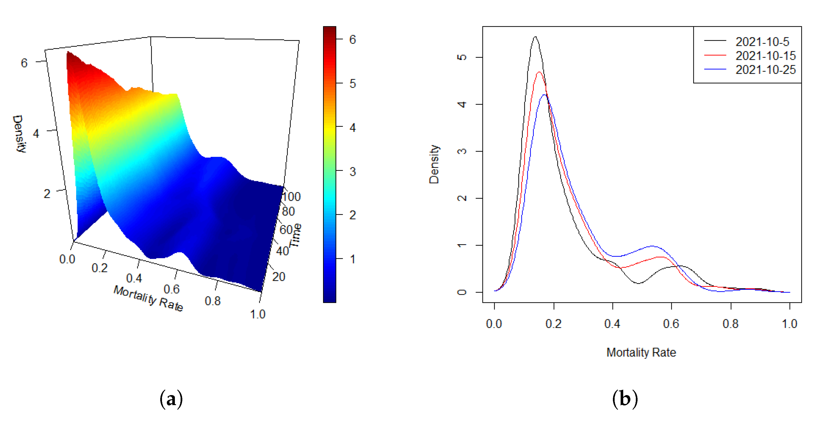
Figure 2.
Average estimations of error process obtained from 200 Monte Carlo runs with sample size and observations. Picture (a): true curves, (b): spline estimations.
Figure 2.
Average estimations of error process obtained from 200 Monte Carlo runs with sample size and observations. Picture (a): true curves, (b): spline estimations.

Figure 3.
Average estimations of . Left panels: true densities, middle panels: initial estimations, right panels: improved estimations. Upper two panels display from two angles, lower panels display .
Figure 3.
Average estimations of . Left panels: true densities, middle panels: initial estimations, right panels: improved estimations. Upper two panels display from two angles, lower panels display .
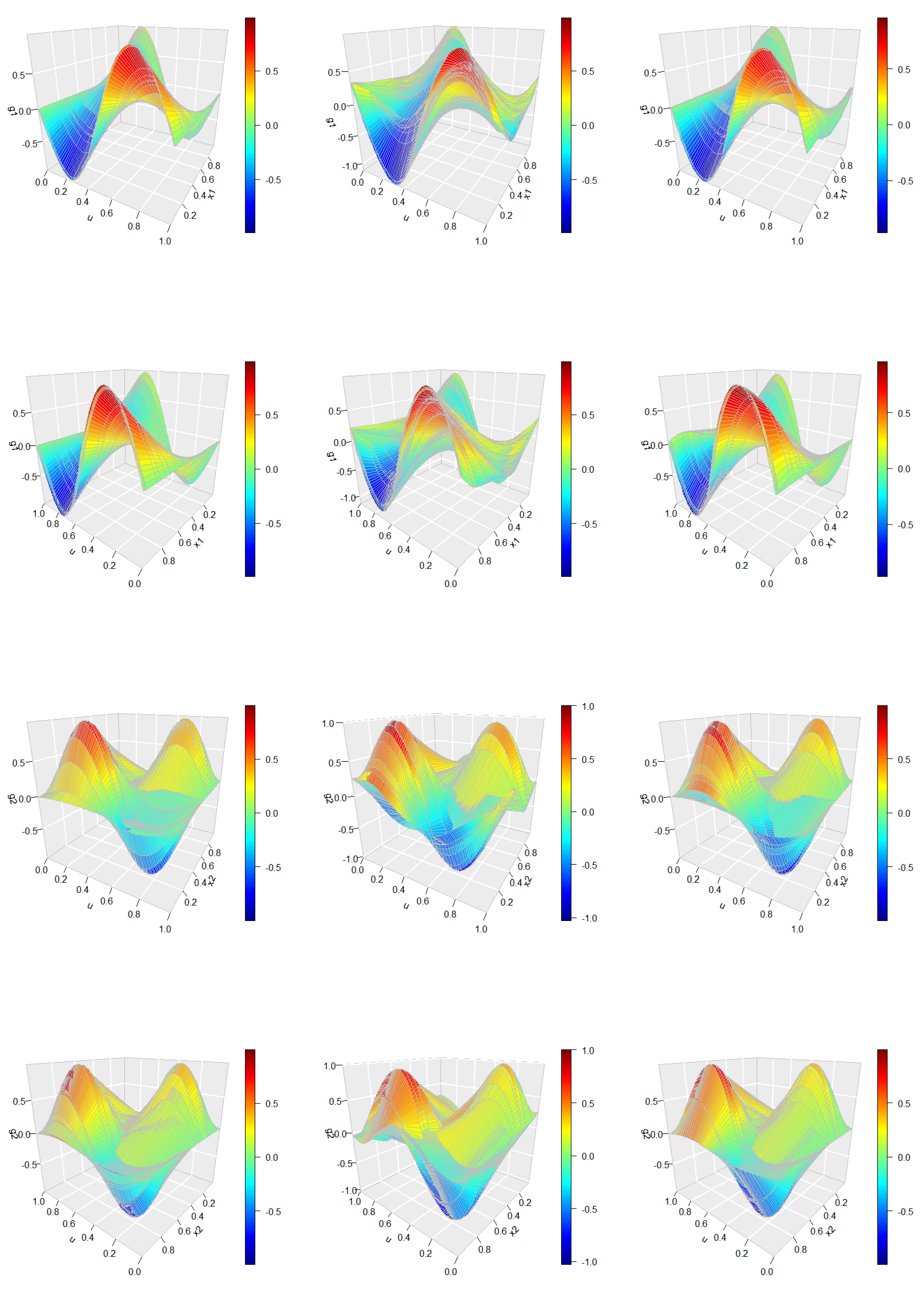
Figure 4.
Heat map of bivariate function in the model based on the mortality rate (‰) data of COVID-19.
Figure 4.
Heat map of bivariate function in the model based on the mortality rate (‰) data of COVID-19.
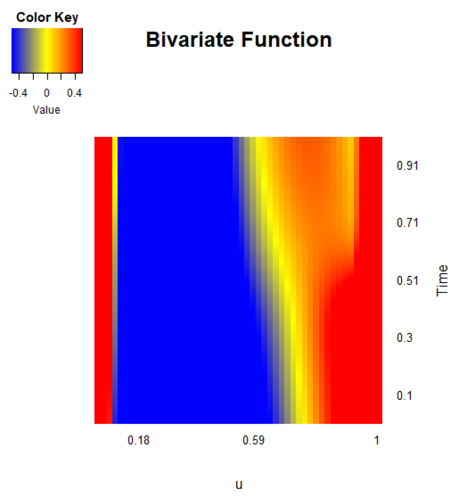
Figure 5.
Densities of national quarterly personal income in the USA over an interval of 44 quarters. (a): Three-dimensional trend of density time series during the whole period; (b): Density curves at three different selected quarters .
Figure 5.
Densities of national quarterly personal income in the USA over an interval of 44 quarters. (a): Three-dimensional trend of density time series during the whole period; (b): Density curves at three different selected quarters .
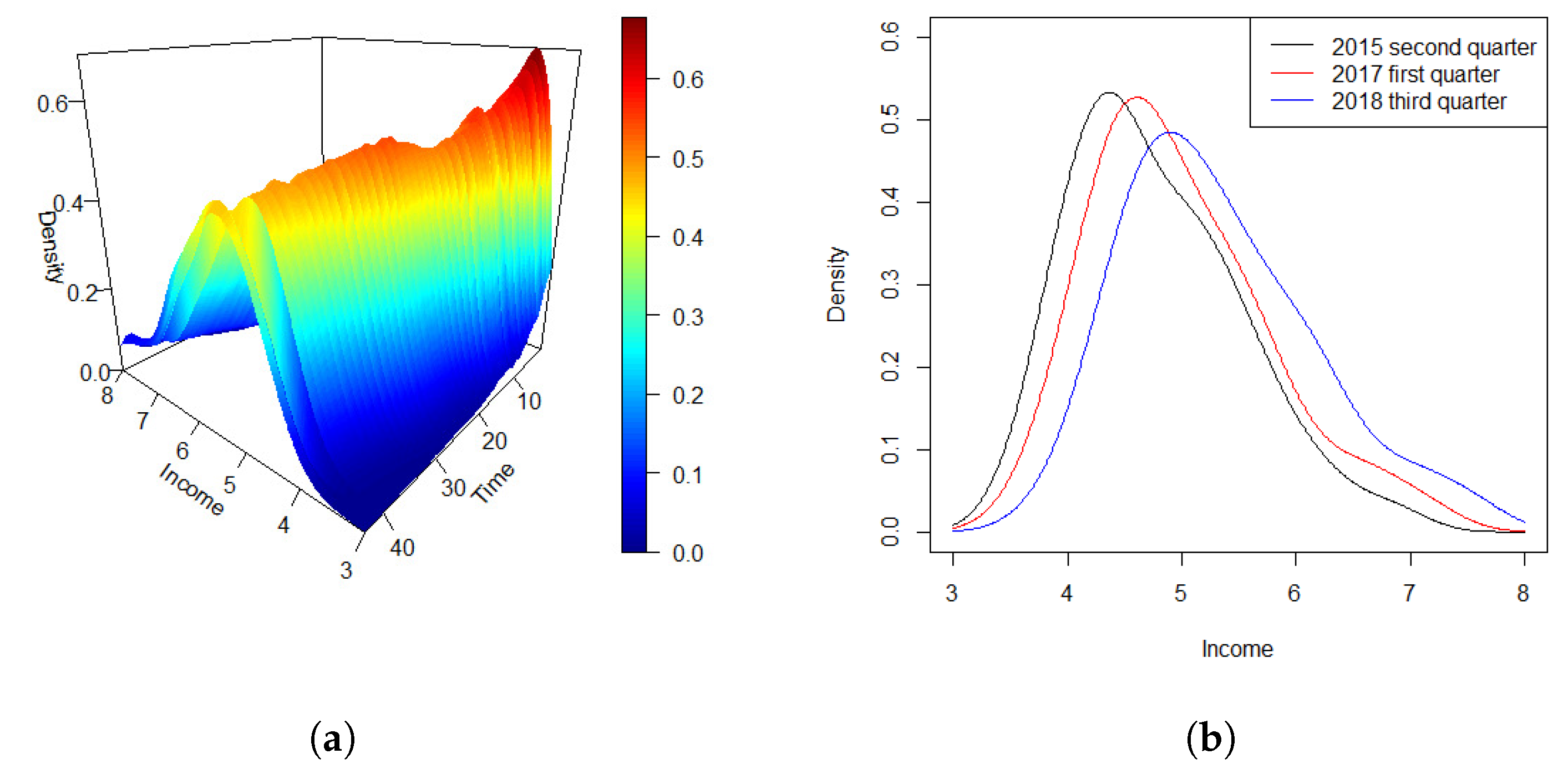
Figure 6.
Heat maps of bivariate varying-coefficient functions in the USA income data model.


Table 1.
Average RMSEs of both initial and improved estimations of .
| Average RMSEs of Bivariate Varying-Coefficient Additive Functions | |||||
| Sample Size | |||||
| T | n | Initial | Improved | Initial | Improved |
| 50 | 50 | 0.2247 | 0.1848 | 0.2139 | 0.1785 |
| 100 | 0.1759 | 0.1325 | 0.1844 | 0.1521 | |
| 100 | 50 | 0.1826 | 0.1471 | 0.1732 | 0.1354 |
| 100 | 0.1431 | 0.1164 | 0.1319 | 0.1057 | |
Table 2.
Average Standard Deviation (SD) and Bias of both initial and improved estimations of .
| Average SD and Bias of Bivariate Varying-Coefficient Additive Functions | |||||||||
| Sample Size | |||||||||
| Initial | Improved | Initial | Improved | ||||||
| T | n | SD | Bias | SD | Bias | SD | Bias | SD | Bias |
| 50 | 50 | 0.205 | 0.147 | 0.168 | 0.104 | 0.219 | 0.137 | 0.183 | 0.117 |
| 100 | 0.179 | 0.122 | 0.142 | 0.093 | 0.196 | 0.128 | 0.164 | 0.095 | |
| 100 | 50 | 0.174 | 0.136 | 0.151 | 0.082 | 0.187 | 0.131 | 0.158 | 0.086 |
| 100 | 0.133 | 0.099 | 0.112 | 0.057 | 0.153 | 0.111 | 0.129 | 0.061 | |
Table 3.
Empirical power of testing algorithm to determine the order of FAR error process under different significance levels.
Table 3.
Empirical power of testing algorithm to determine the order of FAR error process under different significance levels.
| Null Hypothesis | |||||||
| Alternative Hypothesis | |||||||
| Sample Size | Significance Level | Significance Level | Significance Level | ||||
| T | n | 0.05 | 0.1 | 0.05 | 0.1 | 0.05 | 0.1 |
| 50 | 50 | 0.893 | 0.962 | 0.787 | 0.846 | 0.082 | 0.134 |
| 100 | 0.931 | 0.985 | 0.824 | 0.893 | 0.073 | 0.125 | |
| 100 | 50 | 0.942 | 0.972 | 0.821 | 0.881 | 0.071 | 0.121 |
| 100 | 0.985 | 1.000 | 0.889 | 0.935 | 0.064 | 0.113 | |
Table 4.
Average RMSEs of both initial and improved estimations of .
| Average RMSEs of Bivariate Varying-Coefficient Additive Functions | |||||
| Sample Size | |||||
| T | n | Initial | Improved | Initial | Improved |
| 50 | 50 | 0.2739 | 0.2438 | 0.2691 | 0.2235 |
| 100 | 0.2264 | 0.1852 | 0.2157 | 0.1809 | |
| 100 | 50 | 0.2136 | 0.1817 | 0.2232 | 0.1761 |
| 100 | 0.1729 | 0.1263 | 0.1816 | 0.1224 | |
Table 5.
P-values of the testing algorithm for identifying the order of functional error process based on the mortality rate data of COVID-19.
Table 5.
P-values of the testing algorithm for identifying the order of functional error process based on the mortality rate data of COVID-19.
| Null Hypothesis | ||
| Alternative Hypothesis | ||
| P-value | 0.000 | 0.194 |
Table 6.
P-values of the testing algorithm for identifying the order of the functional error process based on USA income data.
Table 6.
P-values of the testing algorithm for identifying the order of the functional error process based on USA income data.
| Null Hypothesis | |||
| Alternative Hypothesis | |||
| P-value | 0.000 | 0.000 | 0.436 |
Disclaimer/Publisher’s Note: The statements, opinions and data contained in all publications are solely those of the individual author(s) and contributor(s) and not of MDPI and/or the editor(s). MDPI and/or the editor(s) disclaim responsibility for any injury to people or property resulting from any ideas, methods, instructions or products referred to in the content. |
© 2025 by the authors. Licensee MDPI, Basel, Switzerland. This article is an open access article distributed under the terms and conditions of the Creative Commons Attribution (CC BY) license (http://creativecommons.org/licenses/by/4.0/).
Copyright: This open access article is published under a Creative Commons CC BY 4.0 license, which permit the free download, distribution, and reuse, provided that the author and preprint are cited in any reuse.


