
Submitted:
12 August 2025
Posted:
13 August 2025
You are already at the latest version
Abstract
The profound duality between the distribution of prime numbers and the non-trivial zeros of the Riemann zeta function, $\zeta(s)$, is a cornerstone of analytic number theory. This paper introduces a novel analytical framework, inspired by the principles of signal processing and systems theory, to derive a new product-sum identity that makes this duality explicit. Starting from the second Chebyshev function, $\psi(x)$, we employ a sequence of transforms, complex analysis techniques, and functional manipulations to construct a new function, $\hat{\Psi}(z)$. We prove that this function admits two distinct but equivalent representations: (i) an infinite product whose zeros are located precisely at the logarithmic prime powers, $z=\pm k\ln p$, and (ii) an exponential sum whose argument is explicitly determined by the ordinates of the non-trivial zeros of $\zeta(s)$. This identity provides a new analytical tool for studying the prime distribution and offers a fresh perspective on the spectral interpretation of the zeta zeros. The derivation serves as a case study in applying systems-theoretic thinking to classical problems in number theory, with potential implications for the development of new computational algorithms.
Keywords:
Riemann zeta function
; Chebyshev function
; prime numbers
; explicit formulas
; Cauchy’s Argument Principle
; Laplace transform
; Riemann Hypothesis
; analytic number theory
; signal processing
MSC: 11M06; 11M26; 44A10; 30E20
1. Introduction
The distribution of prime numbers, though seemingly erratic at a local scale, is governed by deep and subtle laws. The seminal work of Riemann [1] established an intrinsic connection between the prime-counting function and the complex zeros of the Riemann zeta function, . This connection is most sharply formulated through explicit formulas, which relate sums over primes to sums over the zeta zeros. The most famous of these, the Riemann-von Mangoldt formula, demonstrates that the fine structure of the prime distribution is dictated by an oscillatory "noise" term composed of contributions from each non-trivial zero of [2]. This establishes a duality that is conceptually analogous to the relationship between a time-domain signal and its frequency spectrum in Fourier analysis.
This analogy has inspired a rich tradition of viewing number-theoretic problems through the lens of physics and systems theory, where the zeta zeros are interpreted as the resonant frequencies or energy levels of a hypothetical quantum system [3] and [4]. While this perspective has been highly influential, it is often presented as a metaphorical or heuristic guide. In this paper, we take this analogy as a formal guiding principle for derivation. We treat the prime distribution as an aperiodic, event-driven signal and apply standard tools from systems theory, primarily the Laplace transform, to analyze its structure.
Our primary contribution is the rigorous derivation of a novel identity for a newly constructed Chebyshev-type function, denoted . This identity takes the form of a product-sum equivalence:
The product side explicitly encodes the locations of prime powers as its zeros, while the sum side is constructed directly from the ordinates of the non-trivial zeros of . This result is not a restatement of existing explicit formulas but a new representation derived through a systematic sequence of transformations. The derivation itself serves to demystify the prime-zero duality by casting it as a concrete problem in transform theory, where the zeros emerge as the spectral signature of the prime signal.
This new formulation has several potential implications. It provides a new analytical object whose properties may be studied to yield further insight into the statistical behavior of primes. Furthermore, the explicit product-sum equivalence may offer a foundation for novel numerical algorithms for prime counting or zero localization.
This new formulation of a Chebyshev-type function offers a unique analytical lens into the long-standing prime-zero duality. It provides a compact and potentially computationally tractable framework for analyzing prime number distribution, opening avenues for deeper analytical investigations into the Riemann Hypothesis, and inspiring the development of novel numerical algorithms for prime counting or zero localization. The structure of this paper is as follows: Section 2 provides necessary preliminaries. Section 3 details the step-by-step derivation of . Section 4 provides a focused discussion of the signal-processing perspective and its implications. Section 5 discusses the properties and implications of the derived function. Finally, Section 6 concludes with a summary of the results and directions for future work.
2. Preliminaries and Background
The second Chebyshev function, , sums the Von Mangoldt function , defined as if for a prime p and integer , and 0 otherwise. It can be conveniently expressed using the Heaviside step function (where for and for ), as:
The Riemann zeta function, , initially defined for by , can be analytically continued to the entire complex plane, having a simple pole at . Its non-trivial zeros are the focus of the Riemann Hypothesis. For analytical convenience, the completed Riemann zeta function, , is defined as
The function is an entire function, and its zeros correspond precisely to the non-trivial zeros of .
Cauchy’s Argument Principle is a powerful tool in complex analysis for counting zeros and poles of a meromorphic function. For an entire function and a simple closed contour that does not pass through any zeros of , the principle states that:
Finally, the Laplace transform
Plays a crucial role in transforming sums over functions into forms amenable to analytical manipulation.
3. Derivation of the z-domain Chebyshev Function
This section details the step-by-step derivation of the novel z-domain Chebyshev function , starting from the classical Chebyshev function and employing a sequence of analytical transformations.
3.1. Laplace Transform
We begin by taking the Laplace transform of the second Chebyshev function , defined in (1). We define its Laplace transform as
Using the linearity of the Laplace transform and the transform of a Heaviside step function (specifically, ), we evaluate the transform of each term:
This leads to the relationship between and a sum over prime powers:
This sum is a well-known Dirichlet series, which is also precisely equal to the negative logarithmic derivative of the Riemann zeta function [9]. Thus, we identify the relationship:
The s-domain function has poles at (from ), , (from the pole of ), and at the non-trivial zeros of .
3.2. Inverse Laplace Transform
Lemma 3.1
(Contour closure). Let . For any and , the inverse Laplace transform
can be evaluated by closing the contour to the left and summing residues at the poles of .
Proof.
From the classical bound
uniformly for in bounded intervals, we have for fixed and large :
Thus the horizontal integrals on the large rectangle of height T decay as , and the vertical integral on the far left is exponentially small as . Since , Jordan’s lemma ensures that the contribution from the left semicircle vanishes, allowing the contour to be closed to the left. □
Definition 3.1
(Symmetric truncation). For any function g of the zeros of ζ, define
where the zeros ρ are counted with multiplicity and summed in symmetric order with respect to the real axis.
Theorem 3.1.
Let be defined by . For and assuming all zeros of are simple, the inverse Laplace transform is given by the symmetric truncation identity
where the sum runs over all non-trivial zeros ρ of and the last sum is over the trivial zeros . Equivalently,
with the pairwise sum over conjugate non-trivial zeros taken in the symmetric truncation sense.
Proof.
By Lemma 3.1, we may close the Bromwich contour for to the left when . The poles of are:
- 1.
- At the pole (simple pole of ):
- 2.
- At non-trivial zeros : Since is simple, has residue 1 at , hence
- 3.
- At trivial zeros : Similarly,
Summing all residues in the closed contour and interpreting the sum over non-trivial zeros in the symmetric truncation sense gives
which is Equation (6). □
Remark: The symmetric truncation in Theorem 3.1 is essential because the raw series does not converge in the usual sense for fixed .
- 1.
- Divergence without regularization. Writing a non-trivial zero as , each term has modulus . Since , these magnitudes do not tend to zero; under the Riemann Hypothesis (), each term has modulus . Thus the partial sums cannot converge absolutely and will generally diverge unless a summation procedure is specified. Symmetric truncation balances contributions from zeros with positive and negative imaginary parts, often producing a conditional or distributional limit.
- 2.
- Relation to more convergent explicit formulas. Classical explicit formulas (e.g., the Riemann–von Mangoldt formula for the Chebyshev function ) involve sums rather than ; the factor improves convergence because as . In the Laplace inversion setting, similar convergence improvement occurs if one differentiates or integrates with respect to u, or pairs the residue expansion with a smooth test function in u. Alternatively, one can insert a factor and remove it after summation, which corresponds to smoothing.
Thus Theorem 3.1 is an algebraically correct residue expansion, but must be interpreted via symmetric truncation or another regularization to define the sum over non-trivial zeros rigorously.
Whereas, the inverse Laplace transform of the term involving , is given by:
Thus, we have
Also, integrating Equation (8) and rearranging with , we obtain:
We can think of as a transfer function. In this view, the logarithmic derivative of the Riemann zeta function is reinterpreted as the transfer function of a linear system. It encodes how the system responds to inputs, transforming a purely theoretical object into a dynamic model with physical intuition of prime powers as impulse train signal. Resonant frequencies at the poles: The poles of correspond to the system’s natural modes, frequencies at which it naturally oscillates when excited. This reframes each pole as a physical resonance. Thus, the pole at : Represents an unstable exponential mode, . Poles at non-trivial zeros , these define damped oscillatory modes; is the oscillation frequency, whereas is the damping factor. Here, the Riemann Hypothesis gains a striking physical interpretation: if all , then every oscillatory mode decays at the same rate. This enforces a uniform damping structure, turning what could be chaotic decay into a coherent harmonic spectrum: the "music of the primes."In essence, it recasts a central problem in number theory through the lens of system dynamics, bridging abstract mathematics with the language of engineering and physics.
Equation (8) is the positive part of the explicit formulas established by Weil [8]. The derivation above provides a powerful illustration of the deep connection between prime numbers and the zeros of the Riemann zeta function from both theoretical and physical interpretation. The transformation technique can be summarized in four conceptual steps.
- 1.
- Encoding: The raw, discrete distribution of prime powers is first encoded as a series of spikes (delta functions) on a logarithmic scale.
- 2.
- Transformation: The Laplace transform acts as a bridge, converting this discrete distribution into a single analytic function in the complex plane, as: .
- 3.
- Spectral Decomposition: In this new domain, complex analysis allows this same function to be re-expressed not in terms of primes, but as a sum over its fundamental poles, which are precisely determined by the zeros of .
- 4.
- Inverse Transform: The final inverse Laplace transform translates this "spectral data" of the zeros back into the original domain, revealing that the prime distribution is composed of a main growth term (from the pole at ) plus oscillatory "correction" terms dictated by the non-trivial zeros.
This process provides an explicit duality, demonstrating that the distribution of prime numbers is governed by the harmonic structure of the zeros of the zeta function.
The novelty of this approach lies not in discovering a new mathematical truth, but in a powerful translation that makes a classic result conceptually clear and accessible. While the explicit formula is traditionally derived using the abstract machinery of complex contour integration, this methodology reframes the entire problem in the language of signal processing. By treating the prime distribution as a "signal" and applying the Laplace transform, the derivation becomes a familiar exercise in systems theory. This conceptual shift demystifies the process, revealing the zeros of the zeta function to be the fundamental "resonant frequencies" that govern the seemingly chaotic structure of the primes. The true innovation is therefore explanatory: it recasts an obscure theorem into an intuitive spectral decomposition, bridging the gap between pure number theory and the world of applied science and engineering.
3.3. Explicit Formula from Contour Integration
We invoke Cauchy’s Argument Principle to relate the counting function for non-trivial zeros to a contour integral involving the completed Riemann zeta function . Let denote the number of non-trivial zeros of with positive imaginary parts . The closed contour is chosen to encompass the critical strip from imaginary part to . The integral of the logarithmic derivative of over this contour counts all zeros within . Given the symmetry of non-trivial zeros about the real axis, the total number of zeros enclosed by is . Hence,
The integrand on the right-hand side (RHS) is exactly . By Cauchy’s Argument Principle, the RHS evaluates to , which is consistent with the left-hand side (LHS).
The number of zeros is also famously related to the argument of the -function evaluated on the critical line. Specifically, by applying the Argument Principle over a contour enclosing the critical strip and utilizing the symmetry properties of , one derives the standard result (see, e.g., Titchmarsh [5], Chapter IX):
where the argument is defined by continuous variation from a reference point on the real axis (e.g., ) where . This formula holds precisely if is not the ordinate of a zero. The term is the imaginary part of . Since is real for real s, we have . Consequently, the difference of logarithms becomes:
Therefore, we can express the counting function as:
We now evaluate the term on the RHS using the definition of :
Evaluating this difference at and , we have:
For large , we use the asymptotic behavior of complex logarithms and the Stirling approximation for the Gamma function. The terms involving and simplify using for arguments near or . Thus, we have:
Additionally, Stirling’s approximation for the Gamma function logarithm yields (see, e.g., [10]):
Substituting these approximations into the equation for and simplifying, we obtain:
Further simplification leads to:
Thus, we can define the exact explicit Riemann-von Mangoldt zeta zeros count function formula in the -domain [11], as
The derivation of explicit formulas using contour integrals, can be conceptually viewed as a form of inverse transform. This method effectively "inverts" a Dirichlet series (like ) by integrating along specific contours in the complex plane, akin to inverse Laplace transforms with finite limits instead of infinite limits.
Now, the logarithm of the Riemann zeta function can be expressed through its Euler product [9] Chapter 4, as:
Substituting this expansion into the difference term for , we obtain:
Combining these results, we obtain an explicit formula for the zero-counting function in terms of the prime power harmonics, as:
3.4. The Delta-function Density
We differentiate Equation (20) with respect to . The Heaviside sum on the LHS transforms into a sum of Dirac delta functions, representing the density of zeros along the imaginary axis.
Rearranging terms and dividing by i, we obtain a precise explicit formula for the density of non-trivial zeros:
The relationship between Equation (8) and Equation (22) represents a profound duality, forming the mathematical core of the connection between primes and zeta zeros. The first formula, a "prime-centric" view, expresses the distribution of prime numbers as a sum over the zeros of the zeta function. It answers the question, "Where are the primes?" by using the "spectral data" of the zeta zeros. In stark contrast, the second formula provides the dual "zero-centric" view: it expresses the distribution of the heights of the zeta zeros as a sum over the prime numbers. It answers the question, "Where are the zeta zeros?" using the primes as the fundamental frequencies. This elegant reciprocity implies that the two sets of numbers—the primes and the zeta zeros—are inextricably locked together, like a signal and its Fourier transform. All the information about one set is perfectly encoded in the other. This duality is the basis for the modern perspective of number theory through physics, suggesting that the zeros are like the resonant energy levels of a quantum system whose structure is determined by the primes, which act like a classical potential.
3.5. Transformation to the z-domain
We now apply the Laplace transform with respect to to Equation (22). Let z be the Laplace variable. The Laplace transform of is . Thus, we have:
To uncover a product form, we perform a manipulation by considering z as a complex variable. Replacing z by and in the above equation, we obtain two related expressions:
and
Subtracting the first of these two equations from the second, we obtain:
Noting that by assuming . Thus, simplifying the logarithmic term on the RHS, and multiplying the entire equation by i and dividing throughout by 2, we obtain:
Finally, using the identity and , the LHS can be expressed in terms of sine, as:
3.6. Log-Product Form
For the RHS:
For the sum term, we use the integration rule , which can be expressed as when appropriate branch cuts are chosen and assuming the integration constant is zero. Thus, we have:
3.7. Exponentiation and Definition
We now exponentiate both sides of Equation (29) to obtain a product representation. We define the z-domain second Chebyshev function as:
This product form for reveals a fascinating property: its zeros are precisely located at for all prime numbers p and positive integers k. These are the logarithmic prime powers, demonstrating a direct encoding of prime number information.
Noting that the identity for was derived under the condition . To justify its validity across the entire complex plane, we invoke the principle of analytic continuation. Both the product representation of and its exponential sum form define functions that are analytic on the complex plane. Since these two analytic functions have been proven to be equal on the open right half-plane, a domain which contains limit points, the Identity Theorem for analytic functions guarantees that they must be identical everywhere. This rigorously extends the equality from the right half-plane to the entire complex plane, confirming that the function’s zeros are indeed located at .
3.8. The x-domain Representation
Finally, by substituting into the definition of , we obtain its representation in the x-domain:
The zeros of are thus at and (for ), which is consistent with the zeros at .
The exponential form on the RHS of (31), given by
where
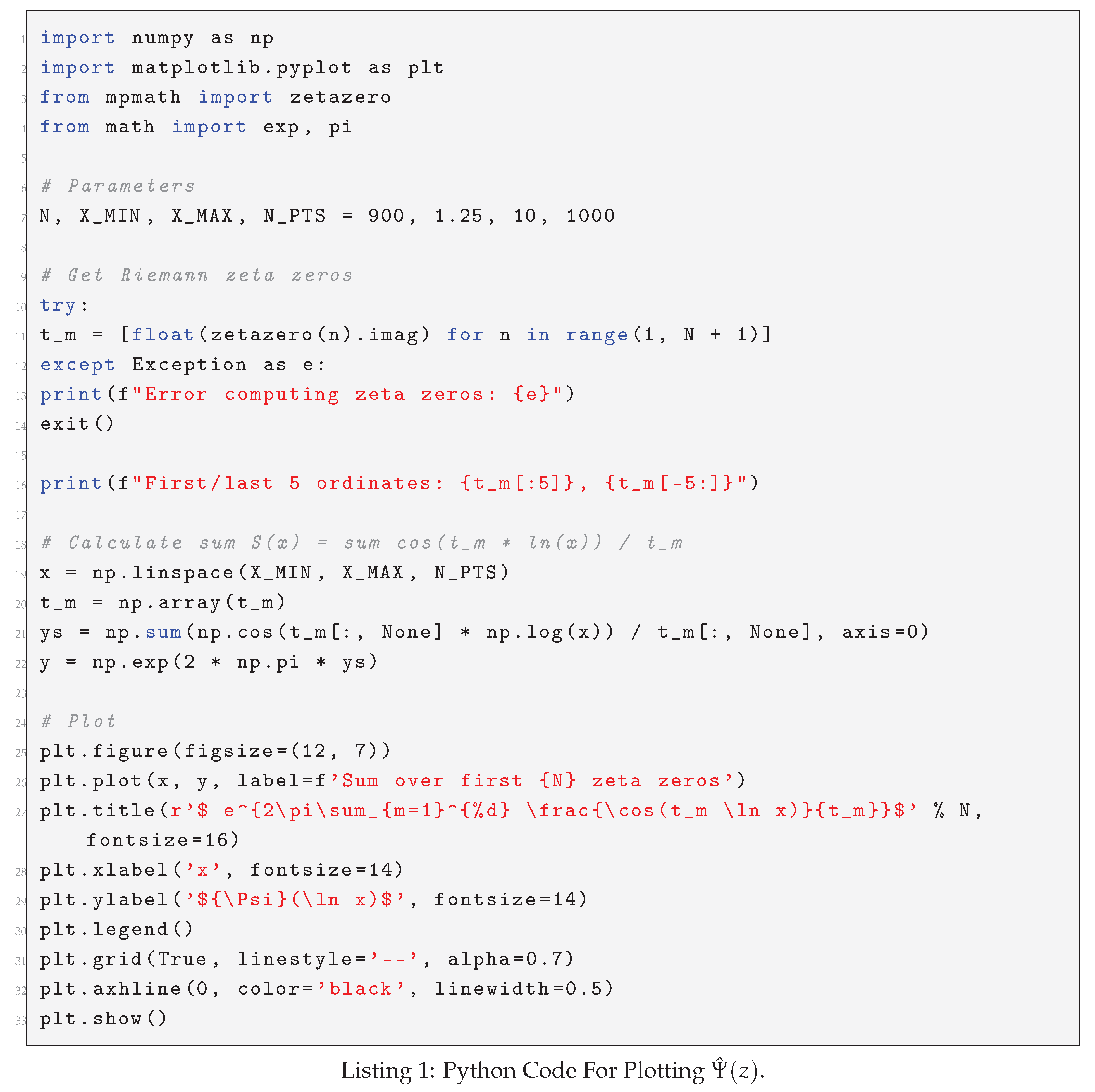
yields a real-valued function for real x. This implies that is always real. Its positivity depends on the sum . The product form clearly shows that if for some prime p and integer k. This occurs when , leading to or . At these specific points, the sum in the exponent must diverge to , driving to zero. This behavior is clearly illustrated in Figure 1, showing sharp dips towards zero at prime power values of x. The corresponding plot of in Figure 2 confirms these divergences as sharp poles towards .
4. A Signal-Processing Perspective
The apparently irregular distribution of the prime numbers can be viewed through the lens of signal processing. In this language the prime-counting “signal’’ and the “spectrum’’ defined by the non-trivial zeros of the Riemann zeta-function, , are dual objects, exactly as a time-domain signal and its frequency response are related by a transform. We have proved the relationships between the three functions, Equations (5), (9) and (30), via employing fundamental tools from complex analysis, Laplace transforms, Cauchy’s Argument Principle. The technique demonstrates transparently the duality between the prime numbers and the ordinate of the zeta non-trivial zeros.
4.1. The Prime-Counting Signal
A natural signal that records the location of prime powers is the Chebyshev function
where term due to zeta trivial zeros, , is negligible and has been omitted from the above expressions.
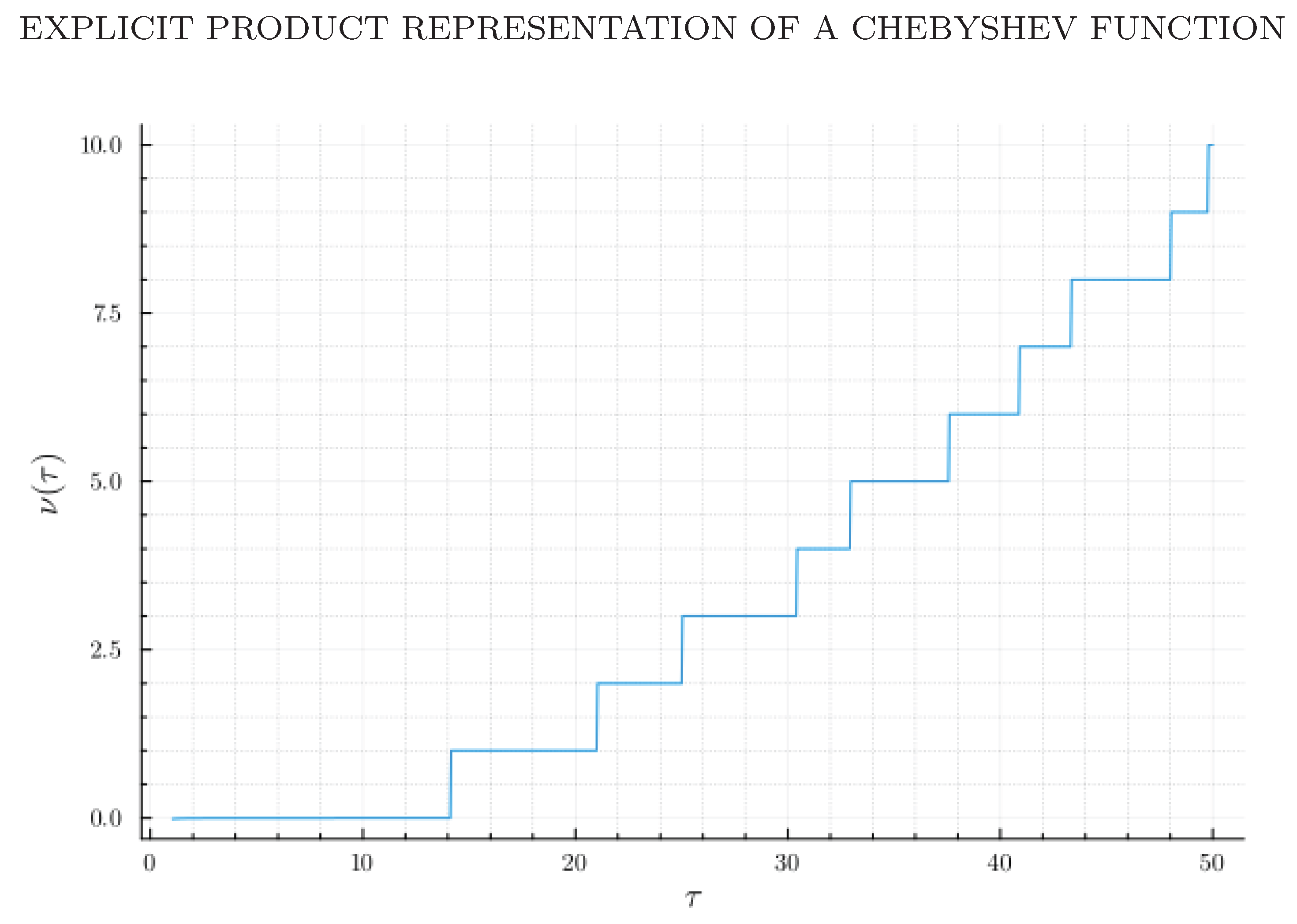
From a signal-processing viewpoint is an aperiodic, stair-case function, see Figure 3, and the differential of this function, yields an impulse train event-driven signal : an impulse of weight, , occurs at each prime power . Understanding the structure of this irregular signal is the central analytic-number-theoretic problem.
The Laplace transform of the derivative , the underlying impulse train, gives:
The sum runs over all non-trivial zeros of . Interpreting the terms in Equation (33) yields the following signal-processing elements:
- Signal : the prime-counting staircase.
- DC componentx: the average (linear) trend, i.e. the Prime Number Theorem.
- AC components : complex exponentials. The ordinates act as fundamental frequencies, while the real parts control growth; () or decay () of the corresponding mode.
If the Riemann hypothesis holds, then for every non-trivial zero; in the signal language this means that all spectral modes are undamped (pure tones), and the fine structure of the prime signal is a superposition of lossless oscillations. The sharp nulls in Figure 4 at are precisely the fundamental frequencies .
Consequently the poles of this transform, i.e. the zeros of , play the role of characteristic frequencies of the prime-distribution system. In Figure 4, which can be interpreted as the magnitude of the system’s frequency response evaluated on the critical line .
4.2. Zeta Zero-Counting Signal
The duality becomes precise through the Riemann–von Mangoldt exact explicit zeta zeros count function formula in the -domain, obtained via the contour integral, Equation (17), as:
Also, in terms of the primes, as:
with the differential, as:
Here, we observe that from a signal-processing viewpoint the function is an aperiodic, event-driven signal: an impulse of one, occurs at each , the ordinate of the zeta zeros.
The sum runs over all prime powers . Interpreting the terms in Equation (36) yields the following signal-processing elements:
- Signal : the zeta zero-counting staircase.
- DC component : the average trend; i.e. the Riemann–von Mangoldt approximate formula.
- AC components : complex exponentials. The prime powers act as fundamental frequencies.
Figure 5.
Plot of .
The Laplace transform of the zero-density signal i.e. the underlying impulse train, see Section 3.5, leads to the function as follows:
4.3. Remark
Viewing the prime-counting function as a signal and the zeros of as its spectral content provides a compact and intuitive framework for many classical results (e.g., the Prime Number Theorem, error terms, and the Riemann hypothesis). This duality suggests that techniques from harmonic analysis and system theory can be imported into analytic number theory, and conversely that number-theoretic phenomena may inspire new signal-processing concepts. Table 1 summarizes the correspondence between the two domains.
5. Discussion and Implications
The derived identity for (Equation (30)) stands as a powerful testament to the profound duality between prime numbers and the non-trivial zeros of the Riemann zeta function. On one side, we have a product whose zeros are explicitly defined by the logarithmic prime powers, . On the other, we have an exponential sum directly involving the ordinate of the zeta zeros. This duality is a cornerstone of analytic number theory, and this novel representation offers a fresh analytical perspective.
This new formulation of a Chebyshev-type function opens several avenues for further theoretical and computational exploration:
-
Computational Algorithms: This identity might inspire novel numerical algorithms for:
- -
- Prime Counting Functions: The direct appearance of prime powers as zeros of could lead to new methods for evaluating or approximating prime-counting functions more efficiently, perhaps by analyzing the local behavior of around its zeros.
- -
- Numerical Stability: Comparative studies of the numerical stability and convergence rates of evaluating (or its x-domain counterpart) via its product form versus its exponential sum form could be highly valuable for practical applications.
- Generalizations: The methodology employed, a sequence of Laplace transforms, differentiation, integration, and exponentiation of explicit formulas, could potentially be generalized to derive similar product-sum identities for other arithmetic functions or for L-functions associated with different number fields. This suggests a broader framework for understanding the interplay between number-theoretic objects and the spectral properties of their associated L-functions.
- Bridging Disciplines: The explicit connection shown by between number theory and the analysis of generalized functions (Dirac delta) and integral transforms underscores the interdisciplinary nature of mathematical research.
Finally, it is remarkable that the final expression for is decorated with the fundamental constants , e, and . Their appearance is not coincidental but rather a profound signature of the underlying mathematical structure. The constant arises from the geometry of the complex plane and the periodicity inherent in the zeta function’s functional equation. The constant e is the bedrock of continuous growth and analysis, underpinning the entire framework of logarithms and exponentials. Finally, the Euler-Mascheroni constant emerges as an intrinsic fingerprint of the Gamma function, which is essential for the analytic continuation of . The presence of this trio confirms that is a natural object, intrinsically linking the discrete world of primes to the fundamental constants of continuous analysis.
6. Conclusion
In this paper, I have rigorously derived a novel product-sum identity for a Chebyshev-type function, . The identity directly equates a product whose zeros are determined by the prime numbers to an exponential sum constructed from the non-trivial zeros of the Riemann zeta function. The derivation was systematically guided by a signal-processing framework, treating the prime distribution as a signal and the zeta zeros as its spectral content. This approach not only yields a new and elegant mathematical formula but also serves as a powerful pedagogical tool for illuminating the profound duality that lies at the heart of analytic number theory.
The result, , stands as a new analytical object whose structure explicitly encodes the relationship between these two fundamental sets of numbers. This work opens several avenues for future research. Theoretically, the properties of could be further investigated to study the statistical nature of primes. Computationally, the dual representation may inspire the development of new numerical methods for prime-counting or for analyzing the distribution of zeta zeros. By framing a classical problem in the language of systems theory, this work underscores the value of interdisciplinary approaches and provides a concrete example of how transform methods can be used to uncover and elucidate deep mathematical structures.
Appendix A Python Code
References
- B. Riemann, Ueber die Anzahl der Primzahlen unter einer gegebenen Grösse, Monatsberichte der Berliner Akademie, (1859), pp. 671–680.
- H. von Mangoldt, Zu Riemanns Abhandlung "Ueber die Anzahl der Primzahlen unter einer gegebenen Grösse", J. Reine Angew. Math., 114 (1895), pp. 255–305.
- M. V. Berry and J. P. Keating, The Riemann zeros and eigenvalue asymptotics, SIAM Rev., 41 (1999), pp. 236–266.
- A. Connes, Trace formula in noncommutative geometry and the zeros of the Riemann zeta function, Selecta Math. (N.S.), 5 (1999), pp. 29–106. Also available as arXiv:math/9811068.
- E. C. Titchmarsh, The Theory of the Riemann Zeta-Function, 2nd ed., D. R. Heath-Brown, ed., Oxford University Press, New York, 1986.
- G. H. Hardy and J. E. Littlewood, Contributions to the theory of the Riemann zeta-function and the theory of the distribution of primes, Acta Math., 41 (1918), pp. 119–196.
- A. Selberg, An elementary proof of the prime-number theorem, Ann. of Math., 50 (1949), pp. 305–313.
- A. Weil, Sur les formules explicites de la théorie des nombres premiers, Comm. Sém. Math. Univ. Lund [Medd. Lunds Univ. Mat. Sem.], Tome Supplémentaire (1952), pp. 252–265.
- H. Davenport, Multiplicative Number Theory, 3rd ed., H. L. Montgomery, ed., vol. 74 of Graduate Texts in Mathematics, Springer-Verlag, New York, 2000.
- H. M. Edwards, Riemann’s Zeta Function, Academic Press, New York, 1974.
- F. Alhargan, An elegant exact explicit formula for Riemann zeta zero-counting function, preprint, 2022, OSF Preprints, https://osf.io/preprints/osf/9su2b.
Figure 1.
Plot of illustrating its positivity and sharp dips towards zero at .
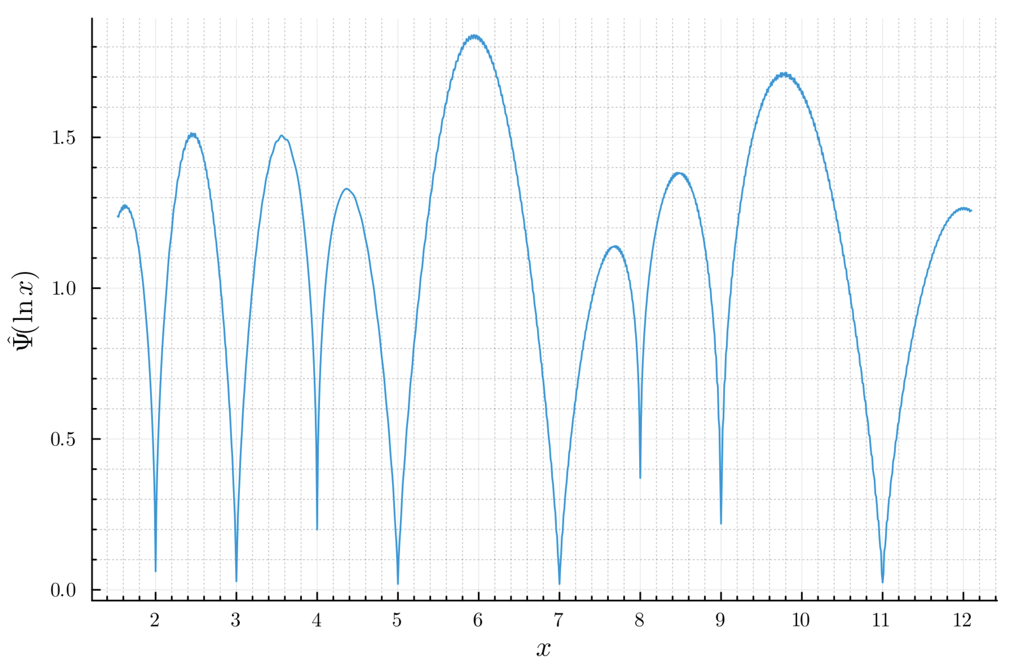
Figure 2.
Plot of illustrating its sharp poles towards at .
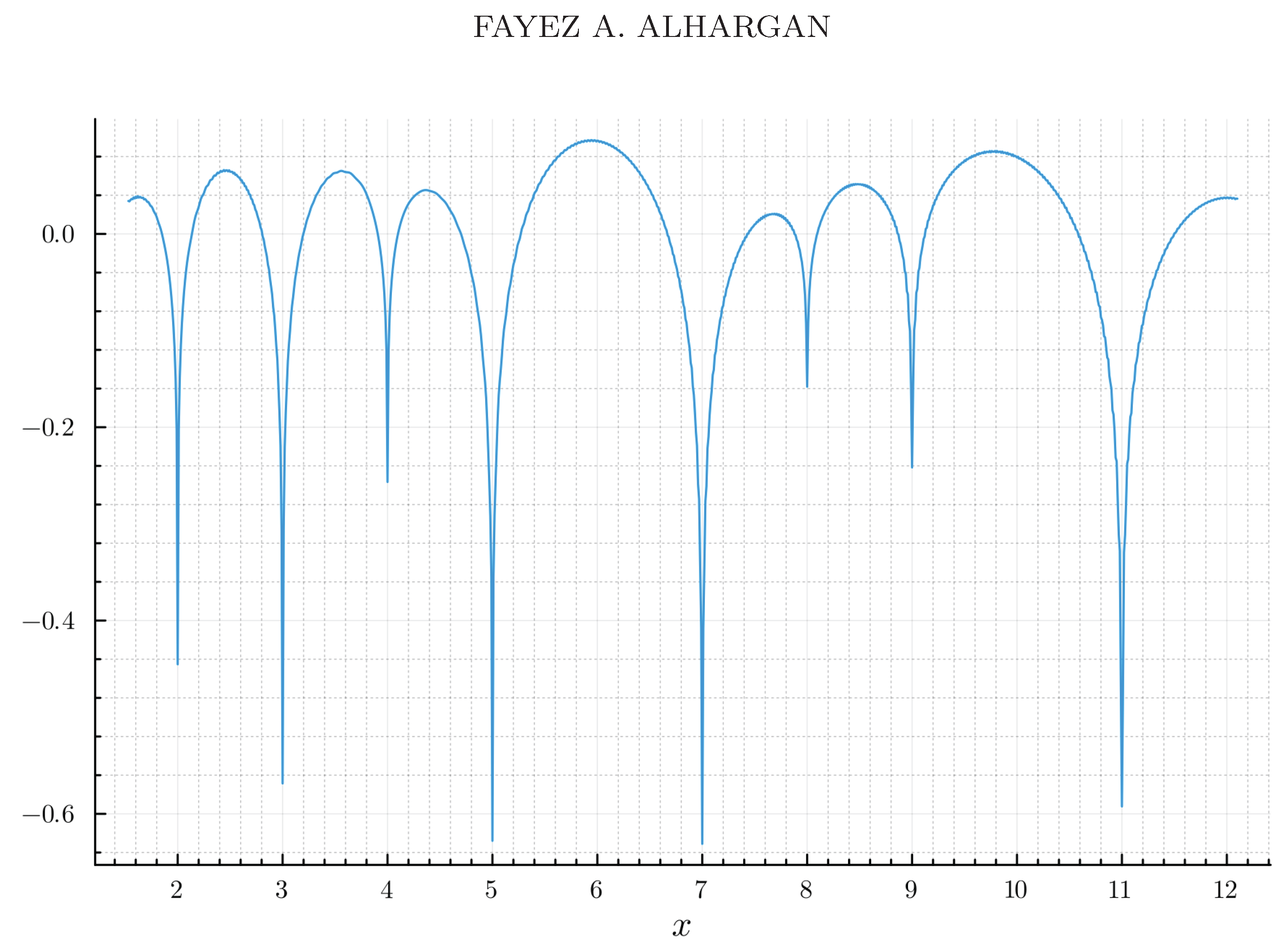
Figure 3.
Plot of showing a step function at .
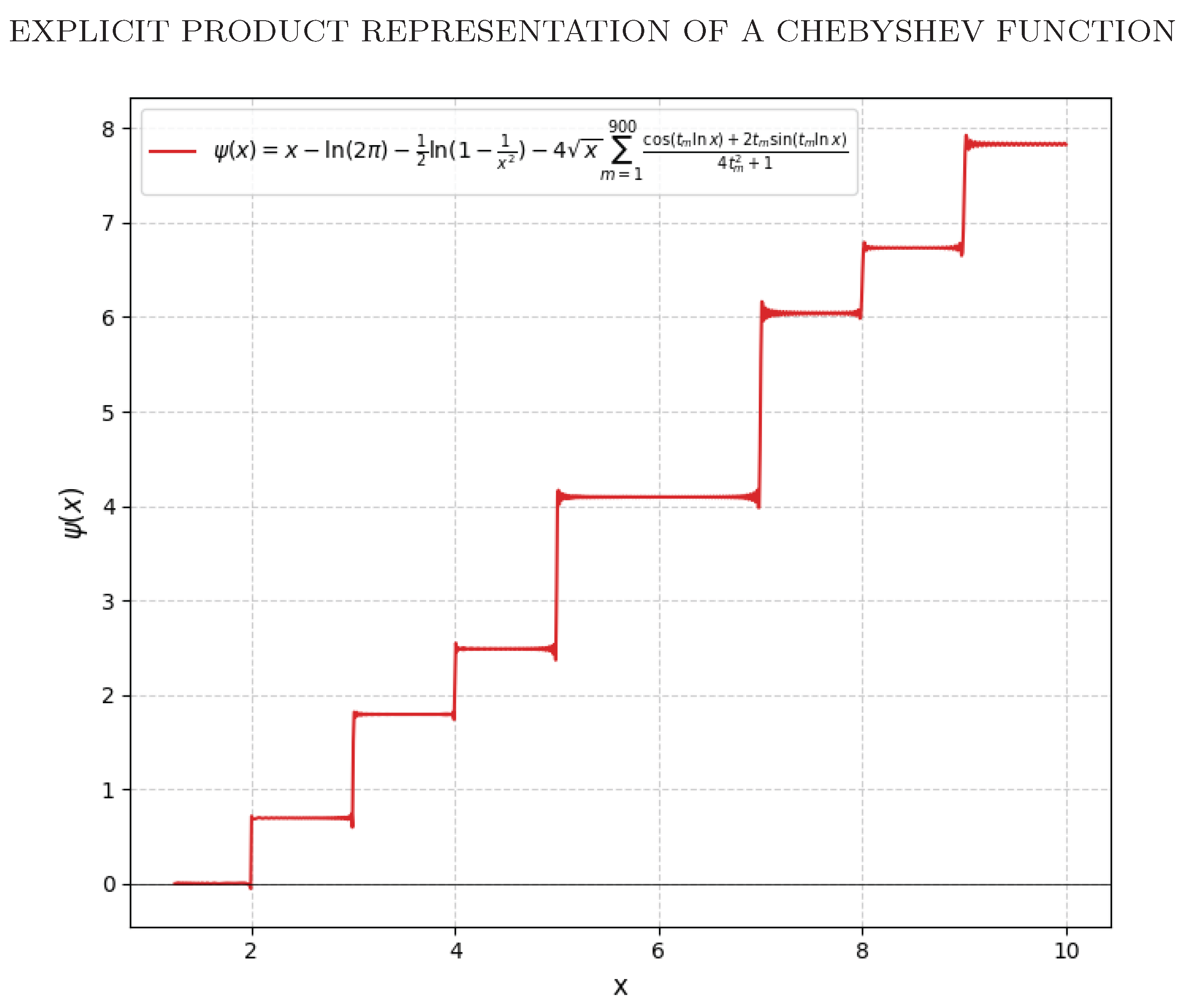
Figure 4.
Plot of along the imaginary axis , showing resonant frequencies at , the ordinate of the zeta zeros.
Figure 4.
Plot of along the imaginary axis , showing resonant frequencies at , the ordinate of the zeta zeros.
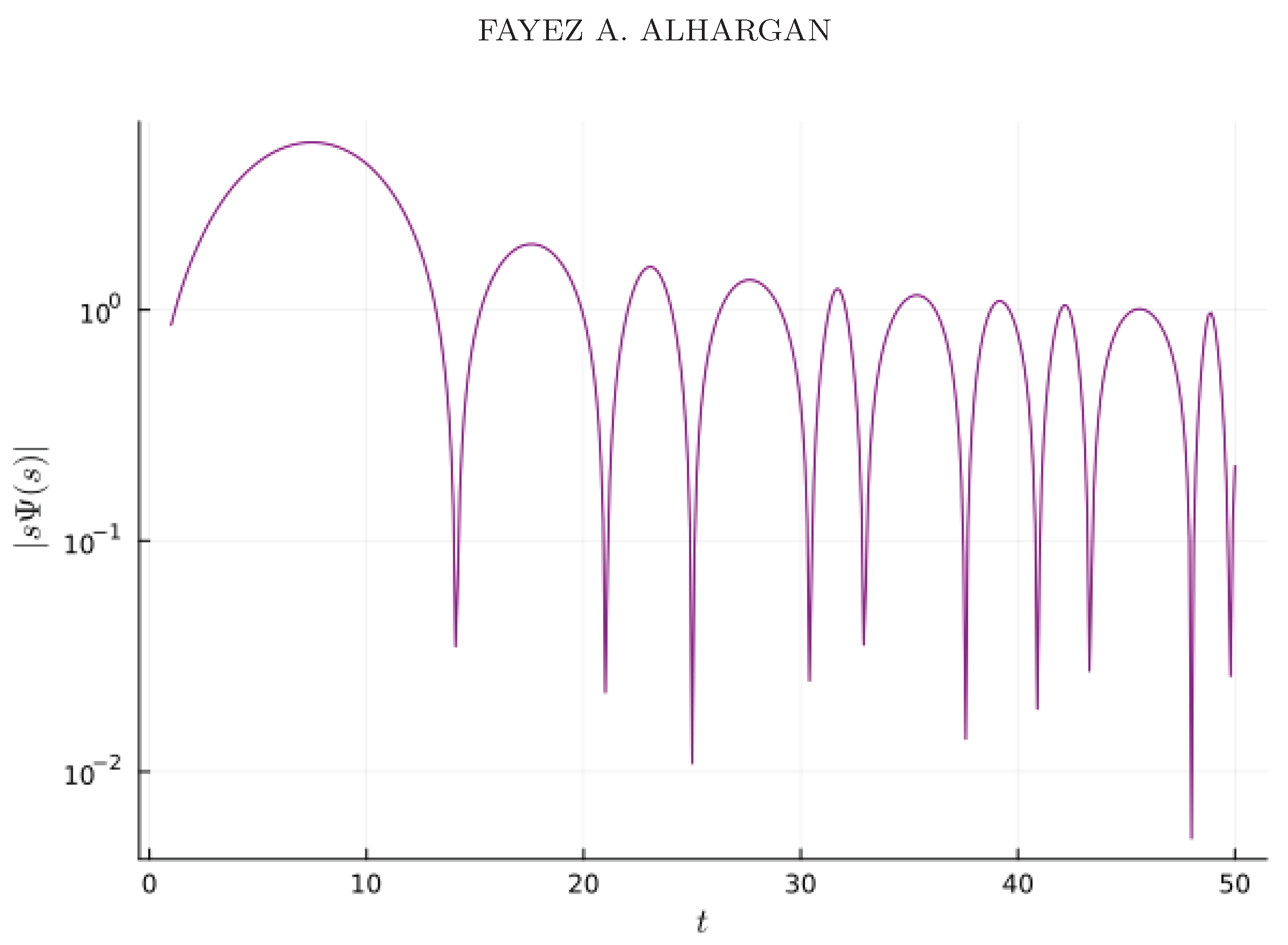
Figure 6.
Plot of illustrating its sharp nulls (zeros) at the logarithmic prime powers ; i.e. resonant frequencies.
Figure 6.
Plot of illustrating its sharp nulls (zeros) at the logarithmic prime powers ; i.e. resonant frequencies.
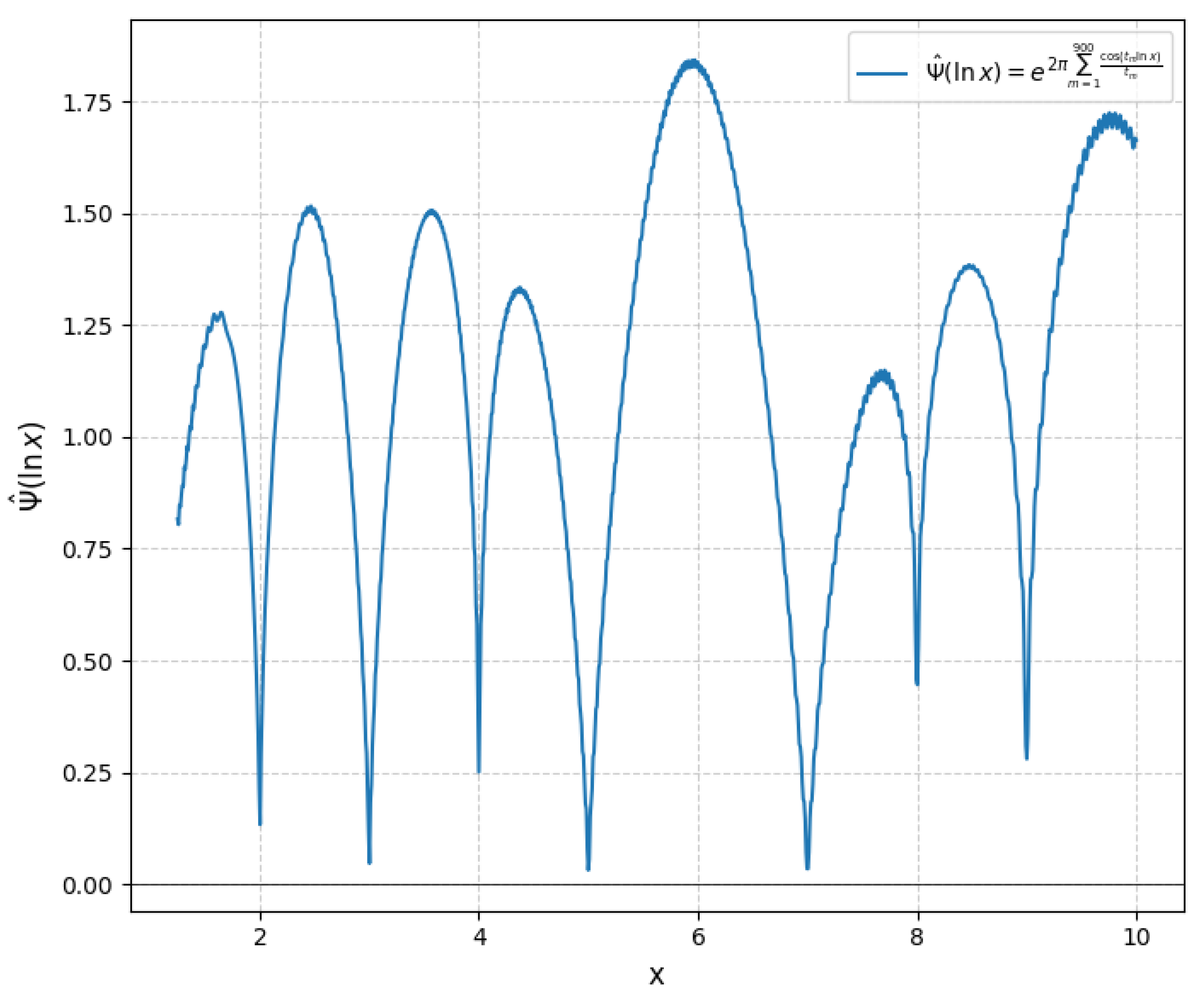

Table 1.
Number-theoretic concepts versus signal-processing analogues.
| Number Theory | Signal Processing |
|---|---|
| Prime-counting staircase | Aperiodic, event-driven signal |
| Non-trivial zeros | Complex frequencies (poles) of the system |
| Ordinates | Fundamental frequencies of the signal |
| Explicit formula (33) | Spectral decomposition / inverse transform |
| Riemann hypothesis () | All spectral modes are undamped (lossless) |
Disclaimer/Publisher’s Note: The statements, opinions and data contained in all publications are solely those of the individual author(s) and contributor(s) and not of MDPI and/or the editor(s). MDPI and/or the editor(s) disclaim responsibility for any injury to people or property resulting from any ideas, methods, instructions or products referred to in the content. |
© 2025 by the authors. Licensee MDPI, Basel, Switzerland. This article is an open access article distributed under the terms and conditions of the Creative Commons Attribution (CC BY) license (http://creativecommons.org/licenses/by/4.0/).
Copyright: This open access article is published under a Creative Commons CC BY 4.0 license, which permit the free download, distribution, and reuse, provided that the author and preprint are cited in any reuse.


