
Submitted:
11 July 2025
Posted:
11 July 2025
You are already at the latest version
Abstract
We employed a global high-resolution inverse model to estimate sectoral methane emissions, integrating observations from the GOSAT-2 satellite for the first time, along with observations from the surface observation network. A similar set of inversions using GOSAT observations was carried out to evaluate the consistency between emissions estimates derived from these two satellites and to ensure that GOSAT-2 data could seamlessly integrate with the existing data series without disrupting the continuity of flux estimates. This analysis, covering the period from 2019 to 2022, utilized prior anthropogenic emissions data mainly from EDGAR v6 and incorporated additional natural sources and sinks as outlined by Saunois et al. (2020). Our analysis reveals a general agreement between total methane emissions estimates from GOSAT and GOSAT-2. However, on a sectoral basis, we found notable regional differences in the flux estimates. While GOSAT inversion estimates ~8 Tg a-1 more anthropogenic emissions for China and around 4 Tg a-1 more wetland emissions for Brazil and Indonesia, the posterior error distribution suggests that GOSAT-2 inversion is closer to surface observations over Asia. These discrepancies are found in regions with significant differences in XCH4 data from the two satellites, such as East Asia and North America, tropical South America, and tropical Africa. These regional biases persist due to limited representative surface reference sites for Level 2 bias correction. The relatively lower data volume from GOSAT also introduces seasonal biases in the flux estimates when the quality filtering of Level 2 data persistently reduces usable observations during certain seasons, resulting in inadequate representation of the seasonal cycle in regions such as East Asia. Similarly, in tropical South America, where the model is relatively under-constrained by the limited surface observations, the lower data volume of GOSAT-2 suffers. While the two inversions exhibit consistent overall performance across North America and Europe, GOSAT-2-based inversion demonstrates a better performance over East Asia. Therefore, while the two satellite datasets are broadly consistent, considering the fact that the biases in the XCH4 data overlap with regions under-constrained by surface observations, establishing additional surface reference measurement sites is desirable to ensure consistent inversion results.
Keywords:
GOSAT
; GOSAT-2
; methane emissions
; sectoral methane emissions
; inverse model
; anthropogenic
1. Introduction
Methane is a potent greenhouse gas that has been increasing at a steeper rate of 8.6 ppb a year during recent years (2011-2020; Liang et al., 2023; Lan et al., 2024). Rising concentrations of methane have contributed to a 0.6°C rise in global temperatures since pre-industrial times (Shen et al., 2023). Hence, the emission mitigation efforts require more realistic emission quantification. Its sources are diverse, encompassing natural processes such as wetlands and geological seepage, as well as anthropogenic activities including agriculture, fossil fuel extraction, and waste management. Effective monitoring and quantification of methane emissions are essential for understanding climate change impacts and guiding mitigation. While bottom-up emission inventories form the basis of these efforts, their accuracy varies by country due to uncertainties. Inverse modeling, which assimilates observations from multiple platforms (e.g., Shen et al., 2023; Nesser et al., 2024), helps assess these emissions. Accurate predictions of future methane growth depend on thoroughly understanding emission sources and processes. Anthropogenic and natural sources contribute by their pathways to the global growth rate. Anthropogenic emissions are influenced by the growing activities in agriculture, fossil fuel exploitation, and waste production. Natural sources, such as wetlands, are, on the other hand, influenced by climate change itself, such as the recent increase in wetland emissions reported by several studies (e.g., Peng et al., 2022; Zhang et al., 2023). National greenhouse gas inventories are fundamental for countries to report their emissions and commitments under international agreements. However, these inventories often rely on uncertain assumptions and sparse ground-based measurements, highlighting the need for independent verification and refinement using advanced observational tools like atmospheric measurements and inverse modeling.
Greenhouse gases Observing SATellite (GOSAT), launched by the Japan Aerospace Exploration Agency (JAXA) in 2009, marked a significant milestone in satellite-based methane observation. GOSAT series are satellites observing atmospheric greenhouse gases jointly developed and operated by the Ministry of the Environment, Japan, JAXA, and the National Institute for Environmental Studies (NIES) (Kuze et al., 2009; Yokota et al., 2009). Equipped with the Thermal And Near infrared Sensor for carbon Observation (TANSO), GOSAT provides XCO2 and XCH4 retrievals for the total atmospheric column. Its successor, GOSAT-2, launched in 2018, builds upon this legacy with improved capabilities, including a slightly higher spatial footprint (9.7 against 10.5km), netter spatial coverage, and enhanced sensitivity to methane emissions. The comparative analysis of GOSAT and GOSAT-2 inversions is pivotal for assessing the consistency and reliability of methane emission estimates derived from these satellites. This comparison not only validates the advancements made in satellite technology but also identifies areas for improvement in future missions. As satellite missions evolve and new technologies emerge, continuity and consistency in methane monitoring are essential for maintaining long-term datasets and ensuring the robustness of emission estimates.
Consistency between space-based instruments is crucial because successor missions (like GOSAT-2) follow their predecessors (like GOSAT). When using such data for emission inversions, ensuring compatibility between datasets from consecutive missions is vital for accurate estimates. Differences due to major improvements in the remote sensing instruments or retrieval algorithms may change the data, but for other reasons, such as systematic errors (biases), ideally, we expect them to be minor so that both datasets have similar information content. As satellite Level 2 products are retrieved from radiance spectra, unlike direct measurements, they need to be corrected for biases based on reference observations. For a similar reason, we also include direct surface-based CH4 measurements from the same surface observation network for both inversions. In this study, we report the results of inverse modeling of GOSAT-2 for the first time and the analysis results of its sectoral comparison with the inversion of GOSAT for the period 2019-2022. Section 2 describes the data used and the methods involved in this study, and section 3 shows the results, including the comparison of sectoral emission estimates, validation with independent observations, and discussion of the causes behind regional inconsistencies, followed by the conclusion.
2. Data and Methods
2.1. Observations
CH4 observations were collected from a network of surface monitoring stations, as compiled in the GLOBALVIEWplus_v4.0_2021-10-14 dataset (Schuldt et al., 2021), with additional data from the ICOS network (ICOS RI, 2021). A list of sites along with site-specific information is given in Table S1 (used for assimilation) and Table S2 (used for validation). Surface sites used in the inversion are also marked in Figure S1a. To ensure that the measurements were representative of well-mixed atmospheric conditions, continuous observations were averaged between 12:00 and 16:00 local time. For high-altitude sites, early morning averages (00:00–04:00 local time) were used to minimize the influence of local emissions transported upslope due to daytime heating. Data uncertainties for surface sites were assessed using the root mean squared error (RMSE) from prior forward simulations, with a minimum threshold of 6 ppb applied to provide greater flexibility for inversion in the Southern Hemisphere. Rejection criteria for surface, aircraft, and ship observations were based on data variance, with a threshold set at double the observed variance.
The satellite observations for this study were obtained from the GOSAT and its successor, GOSAT-2. We utilized the National Institute for Environmental Studies (NIES) Short-Wavelength Infrared (SWIR) bias-corrected Level 2 product V02.95/96 for GOSAT (Yoshida et al., 2013) and the GOSAT-2 NIES full-physics-based bias-uncorrected Level 2 product V02.00 (Yoshida et al., 2023). Yoshida et al. (2023) proposed an empirical formula for correcting the systematic biases in the GOSAT-2 level-2 product. However, for this study, this bias correction has not been applied. Both GOSAT and GOSAT-2 are sun-synchronous satellites, with GOSAT having a revisit cycle of three days and GOSAT-2 a cycle of six days. The TANSO-FTS onboard GOSAT provides observations with a nadir footprint diameter of approximately 10.5 km, while the newer TANSO-FTS-2 (Suto et al., 2021) has a footprint diameter of 9.7 km. TANSO-FTS-2 includes an advanced "intelligent pointing" function, which shifts the instrument's line of sight to avoid clouds detected within its field of view, enhancing the availability of cloud-free data. A plot of one month (October 2019) of GOSAT and GOSAT-2 XCH4 observations is given in supplementary Figure S1.
2.2. Prior Fluxes
Anthropogenic prior fluxes we used were from the Emission Database for Global Atmospheric Research (EDGAR v6, Crippa et al., 2020), excluding emissions from the oil and gas sector. For oil and gas, we used data from the greenhouse gas and air pollution interactions and synergies (GAINS) model (Höglund-Isaksson, 2012). Biomass burning emissions were taken from the Global Fire Emission Database (GFED v4, Randerson et al., 2017). Wetlands and termites were taken from Saunois et al. (2020). Geological and oceanic emissions were taken from Etiope et al. (2019) and Weber et al. (2019), respectively. The methane sink in the soil was taken from MeMo v1.0 (Murguia-Flores et al., 2018). All prior fluxes were provided to the model at 0.1° spatial resolution. Climatological maps of major emission sectors used in the model are given in Figure 1. Monthly climatologies were used for wetlands, geological, termite, and oceanic fluxes. All other fluxes were given at the monthly time step. The prior uncertainties were prescribed as 30% of the climatology of each anthropogenic sector and 50% for wetland emissions.
2.3. Meteorological Data
The meteorological data used for the transport model were obtained from the Japanese Reanalysis (JRA-55; Kobayashi et al., 2015, which provides the required parameters, such as three-dimensional wind fields, temperature, and humidity at 1.25°×1.25° spatial resolution, 40 vertical hybrid sigma-pressure levels, and a temporal resolution of 6 h.
2.4. Inverse Modeling System
2.4.1. NIES-TM-FLEXPART-VAR (NTFVAR) Inverse Modeling System
We utilized a global Eulerian-Lagrangian coupled inverse model known as NTFVAR, which integrates the National Institute for Environmental Studies (NIES) model with FLEXPART (FLEXible PARTicle dispersion model), representing a Eulerian three-dimensional transport model and a Lagrangian particle dispersion model, respectively. The development of this model was documented by Belikov et al. (2016). Our version of the transport model is a modified iteration of the one previously described. This coupled model combines NIES-TM v08.1i, which features a horizontal resolution of 3.75° and 42 hybrid-isentropic vertical levels, with FLEXPART model v.8.0, run in backward mode with a surface flux resolution of 0.1°. The resolution of the Lagrangian model is constrained by the resolution of the available surface fluxes. The current version incorporates revisions to the transport matrix, indexing, and sorting algorithms to enhance memory efficiency for managing large matrices of Lagrangian responses to surface fluxes, particularly for utilizing GOSAT data in the inversion process. Additional details can be found in Maksyutov et al. (2021). Different variants of this model have been used for methane inversion previously (e.g. Wang et al., 2019), but this study uses a modified version used by Janardanan et al. (2024).
2.4.2. The Inverse Modeling Scheme
We employed a high-resolution version of the transport model and its adjoint as detailed by Belikov et al. (2016), combined with the optimization schemes proposed by Meirink et al. (2008) and Basu et al. (2013). Following their methodology, flux corrections were estimated separately for anthropogenic and natural emissions. Variational optimization was utilized to derive two sets of scaling factors for monthly varying prior uncertainty fields at a resolution of 0.1°×0.1°, applied independently to anthropogenic and natural wetland emissions with a bi-weekly time step. Corrections to anthropogenic emissions were based on the monthly climatology provided by EDGAR, while wetland emissions were adjusted according to the monthly climatology from the VISIT model, both of which were defined as prior uncertainty fields. The grid-scale flux uncertainty was set at 30% of EDGAR climatology for anthropogenic emissions and 50% of VISIT climatological emissions for wetland emissions. Other natural flux categories, such as biomass burning, geological sources, termites, and soil sinks, were not optimized due to their significantly lower amplitude compared to wetlands. A spatial correlation length of 50 km and a temporal correlation of two weeks were applied to ensure smooth scaling factors. The inverse modeling problem was formulated to find the optimal values of x, which represent the corrections to prior fluxes, minimizing the cost function J(x).
In this context, H represents the atmospheric transport operator, r denotes the difference between the observed concentrations and the forward simulations conducted using prior fluxes without any corrections, R is the covariance matrix of the observations, and B is the covariance matrix of the prior fluxes. The design of the B matrix involves representing it as a product of a non-dimensional covariance matrix C and a diagonal flux uncertainty matrix D, such that:
𝐵=𝐷𝑇·𝐶·𝐷
The C matrix is typically implemented as a band matrix, where the non-diagonal elements decrease according to ~exp(−l2/d2), with l representing the distance between grid cells and d the correlation distance. The optimal solution, defined as the minimum of the cost function J was determined iteratively using the efficient Broyden–Fletcher–Goldfarb–Shanno (BFGS) algorithm, as described by Gilbert and Lemaréchal (1989). For additional details on the implementation, refer to Maksyutov et al. (2021).
2.4.3. Posterior Uncertainties
Posterior flux uncertainties were calculated from an ensemble of fifteen simulations by randomly perturbing the observations and the prior fluxes, as in the method described by Chevallier (2007). Pseudo-observations were prepared by perturbing the observations with their uncertainty at each site. Also, prior monthly perturbed fluxes were prepared, applying random scaling factors separately for each global carbon project (GCP) region and month. Inversions were carried out using the perturbed pseudo-observations and the perturbed fluxes (perturbed anthropogenic and wetlands with non-perturbed soil sink, biomass burning, and other natural emissions from the ocean, geological sources, and termites) as the prior fluxes and calculating the posterior uncertainty as the standard deviation of the inverted fluxes.
2.4.4. Statistical Significance Test for Difference in Mean
To assess whether the mean flux corrections from the two inversions differ significantly, we performed Welch’s t-test (Welch, 1947) on the monthly flux corrections at 0.1° resolution. The analysis was conducted separately for each of the six optimized source sectors. Results are shown in Figure 2, with hatched areas indicating regions where the differences are statistically significant.
3. Results and Discussion
3.1. Methane Emission Estimates by GOSAT and GOSAT-2 Inversions
Figure 2 illustrates the grid-wise differences in flux corrections inferred from GOSAT and GOSAT-2 inversions to the prior sectoral methane emissions. Statistically significant differences are observed in the agriculture, waste, and wetland sectors, of which the most notable being the lower estimate for wetland emissions. We estimate a mean (2019-2022) global total emission of 605.2 Tg yr-1 for GOSAT and 601.8 Tg yr-1 for GOSAT-2 compared to the prior total of 615.3 Tg yr-1. Table 1 presents the global total sectoral emissions averaged over the study period for the prior and the two sets of inversions. Our estimate is in good agreement with the ensemble mean of the recent global methane synthesis (Saunois et al., 2025). Any mention of emission estimate in the following sections follows the order, GOSAT followed by GOSAT-2. When comparing the sectoral posterior emissions estimated by the GOSAT and GOSAT-2 inversions, there is a noticeable trend: GOSAT-2 generally estimates lower emissions for Southeast Asia (Figure 2) than GOSAT. GOSAT-2 provides lower estimates for the agriculture sector in Southeast Asia, parts of Europe, and tropical America. For instance, in China, GOSAT estimated 23.18±1.54 Tg yr-1 of methane emissions from agriculture, while GOSAT-2 estimated 16.82±1.12 Tg yr-1 (Table 2). This estimate is lower than recent studies, such as the one by Chen et al. (2022) on TROPOMI inversion, which reported 17.8 Tg yr-1 from livestock and 11.9 Tg yr-1 from rice paddies using GOSAT as a reference to omit outliers in the inversion. Therefore, it is reasonable that our GOSAT inversion is on the upper side, closer to Chen et al. (2022). The primary reason for the difference with GOSAT-2 inversion is the lower XCH4 observed by GOSAT-2 over eastern China and the surrounding regions. In contrast, for other regions of the globe, GOSAT-2 inversion estimates higher emissions compared to GOSAT, particularly in central North America, eastern temperate South America (Argentina 2.34±0.25; 2.97±0.31 Tg yr-1, Brazil 13.52±0.36; 14.29±0.38 Tg yr-1), tropical Africa, and Southwest Asia (Pakistan). However, the difference in the posterior agricultural emission in the two inversions for Pakistan is greater than the uncertainty level (5.34±0.37; 5.87±0.41 Tg yr-1).
In the waste sector, the largest emitter is China, with GOSAT estimating 14.36±0.7 Tg yr-1 and GOSAT-2 estimating 13.35±0.65 Tg yr-1, followed by USA (4.29±0.05; 4.62±0.06 Tg yr-1), India (6.56±0.15; 6.44±0.15 Tg yr-1), and Brazil (4.91±0.09; 5.06±0.09 Tg yr-1). GOSAT-2 also estimates lower emissions for Mexico, northern South American countries, and East, South, and Southeast Asia. Generally, GOSAT-2 has a good agreement with GOSAT over Australia, boreal Eurasia, and South Africa, while GOSAT-2 suggests higher emissions over Europe and eastern North America. For the coal sector, GOSAT estimates higher emissions than GOSAT-2 for India, China, Southeast Asia, and Australia. Conversely, GOSAT-2 provides higher emission estimates for the USA, Europe, and Russia. Emissions from coal mining in China are consistent between GOSAT and GOSAT-2 (18.97±0.98 and 18.31±0.95 Tg yr-1, respectively), aligning with recent studies such as Chen et al. (2022), which reported 16.6 Tg yr-1. The differences between the inversions are within the estimation uncertainty for China. Additionally, slight variations in coal emission estimates between the two inversions are observed for Indonesia.
In the oil and gas sector, GOSAT-2 suggests higher emissions from localized sources in the United States, Europe, Russia, the Middle East, and parts of Africa. Conversely, GOSAT estimates higher emissions in Southeast Asian countries. The largest differences between the two inversions are observed for Nigeria (2.08±0.37 Tg yr-1 vs. 2.86±0.51 Tg yr-1), one of Africa’s largest producers, and similar differences are noted for oil and gas producers in the Middle East, such as Iraq and Saudi Arabia. GOSAT-2 estimates higher emissions from major sources in the Middle East, Africa, and the United States. However, at the country level, the differences generally fall within the uncertainties of the inversions.
For wetland emissions, GOSAT estimates higher emissions in Amazonia, Southeast Asia, central Africa, and Australia. Figure 3b illustrates a slight bias remaining in the GOSAT-optimized forward simulation compared to observations in Amazonia and Southeast Asia, in contrast to the GOSAT-2 inversion (Figure 3d). GOSAT-2 suggests higher emissions in Canada, Russia, tropical Africa, and southern South America. The most notable differences at the country level are seen for Brazil (30.50±1.67 Tg yr-1 vs. 26.19±1.44 Tg yr-1), Colombia (6.19±0.35 Tg yr-1 vs. 4.71±0.27 Tg yr-1), and Indonesia (12.12±0.77 Tg yr-1 vs. 7.72±0.49 Tg yr-1). Previous estimates for Brazil's wetland emissions using GOSAT inversions (Janardanan et al., 2020) were higher (e.g., ~39 Tg yr-1), compared to ~13 Tg yr-1 by Tunnicliffe et al. (2020). In the present study with GOSAT and GOSAT-2 inversions, the estimates are 30.5 Tg yr-1 and 26.2 Tg yr-1, respectively. Figure 3d shows that the posterior simulation by GOSAT-2 exhibits less bias over Brazil compared to the optimized forward simulation by GOSAT whereas GOSAT-2 estimates lower emissions in central African countries compared to GOSAT.
In East Asia and adjacent oceanic regions, GOSAT often shows higher XCH4 values, especially over China. Figure 4 highlights this, with some months showing XCH4 values exceeding 30 ppb or more in GOSAT compared to GOSAT-2. This discrepancy may account for the elevated emissions in sectors like Agriculture, Waste, and Coal in the East China region. Figure 3 compares the differences between prior forward and optimized forward simulations of GOSAT and GOSAT-2. It is evident that the prior forward simulation for GOSAT-2 was more biased over North American and Asian regions (Figure 3c, h, j) compared to GOSAT, possibly due to the biases in the GOSAT-2 Level 2 data over North America and Asia (Yoshida et al., 2023). These regions, having a bias in XCH4 data identified by Yoshida et al. (2023), exhibit biases in the prior forward also. The reasons for the spatial and temporal biases in these two datasets are still under investigation.
The analysis of the residual for forward and optimized simulations for GOSAT and GOSAT-2 reveals that both the inversions, on average work well for North America and Europe (Figure 3e, f), but for East Asia, the posterior fit of the surface observations are handled better by GOSAT-2 inversion (Figure 3g). We have analyzed the results for these three regions defined as North America (60-135°W; 15-85°N), Europe (60°E-30°W; 35-72°N), and Asia (60-160°E; 10-75°N) to evaluate the estimated fluxes (Figure 3e-j). The figure shows the spatial distribution and the density curves for prior and optimized residuals for these three regions for GOSAT and GOSAT-2 inversions. The ability of the two inversions to reduce the posterior mean residuals for surface sites over North America is quite similar, and the distribution curves shift to neutral for both inversions. Similar observations can be made over Europe as well, but with almost indistinguishable performance by the two inversions in bias reduction (Figure 3f). The reason behind this is reflected in the analysis by Yoshida et al. (2023) in their bias estimation of GOSAT and GOSAT-2 relative to the TCCON sites over Europe, both satellite products showed similar performance in the region. This means that both inversions could reduce the biases to the same degree. However, for Asia, there is a distinct difference between the two inversions. All other inputs being the same, GOSAT-2 inversion brings the biases to a minimum in this region compared to GOSAT inversion. This means that despite GOSAT being more mature and evolved in the retrieval processes over the years, GOSAT-2 performs well for the Asian region, which is less constrained by the limited surface observations.
Prior forward simulations for GOSAT show differences from GOSAT-2 prior simulations (Figure 3). GOSAT-2 prior residuals are more biased than GOSAT over North America and Asia. But this can be due to a combination of biases in prior emissions and the Level 2 data itself. However, considering the ability of the two inversions to represent the surface observations (Figure 3e, f, g), it is likely that GOSAT-2 inversions perform better for Asia, while GOSAT and GOSAT-2 are similar in Europe and North America.
3.2. Evaluation with Independent Observations
We used a set of observations that were not assimilated in the inversion process to have an independent evaluation of the posterior emissions in the two sets of inversions. The dataset includes surface and aircraft data across the globe. But a lack of coverage over the southern hemisphere generally and in the northern hemisphere over Asia, Africa, and South America is noted. The locations of the data are given in Figure 5a, and additionally, the details are tabulated in the supplementary Table S2. Globally, the two inversions are consistent with similar residual statistics. Prior RMSE and BIAS were 32.1 and -3.95 ppb, respectively, while after optimization by GOSAT, RMSE and BIAS were 30.8 and -4.8 ppb, and with GOSAT-2 were 31.1 and -3.5 ppb. The detailed RMSE and BIAS for each validation site are given in supplementary Figure S4. The probability density plot of prior and optimized residuals of the two inversions shows that the distribution of the residuals shifts closer to zero after optimization (Figure 5b). Moreover, the two inversions have similar posterior residual distributions. However, we found that for the validation sites in Russia and the northeastern USA, the BIAS has increased in both the inversions (Figure S5). Over northern African validation sites, GOSAT-2 optimization has increased BIAS. However, RMSE was found to have generally reduced except over the northeast USA and Mexico regions. The opposite biases in the African region are attributable mainly to the difference in GOSAT and GOSAT-2 level 2 products. Over Russia, we have few ground observations, and the use of the oil and gas emissions from the GAINS model as prior over Russia introduces some unreasonably high posterior emissions for this sector over the region (Table 2). Unfortunately, there is not enough observation coverage over East Asia, Africa, or South America for validation.
In order to check the performance of the models in representing the marine boundary layer latitudinal profile, we sampled our posterior simulations by GOSAT and GOSAT-2 inversions at the same sites as those used in the NOAA marine boundary layer reference. The marine boundary layer reference (MBLR) is a reference of CH4 concentrations (Lan et al, 2023) represented on latitude constructed from air samples of the Cooperative Air Sampling Network (Dlugokencky et al., 2021). It is created by using selected marine boundary layer sites with measurements representative of a large volume of air masses for each trace gas, providing a latitudinally smoothed distribution of CH4. A detailed explanation can be found on the NOAA website https://gml.noaa.gov/ccgg/mbl/mbl.html (Lan et al., 2023). In the northern latitudes, GOSAT-2-based inversions show a better match to the MBLR, but in the southern hemisphere, GOSAT optimization brings the simulation closer to the reference (Figure 5c). However, inversion results for the Southern Hemisphere deviate more from the MBLR due to sparse observational constraints in this region.
3.3. Attribution of Regional Differences in Posterior Emissions
Since the two sets of inversions differ only by the set of satellite observations used, the estimated flux differences can be attributed to the regional differences in the Level 2 products. Another aspect that could influence the estimated flux is the data volume during the 4 years of analysis. That is the representativeness of satellite data in regions not covered by surface observations. Generally, GOSAT-2 has more observations than GOSAT, and sometimes, GOSAT has very little coverage over certain regions during certain times. We will examine the influence of these two aspects on the regional inconsistencies between the two inversions.
3.3.1. Regional Inconsistency Between XCH4 Retrieval Products
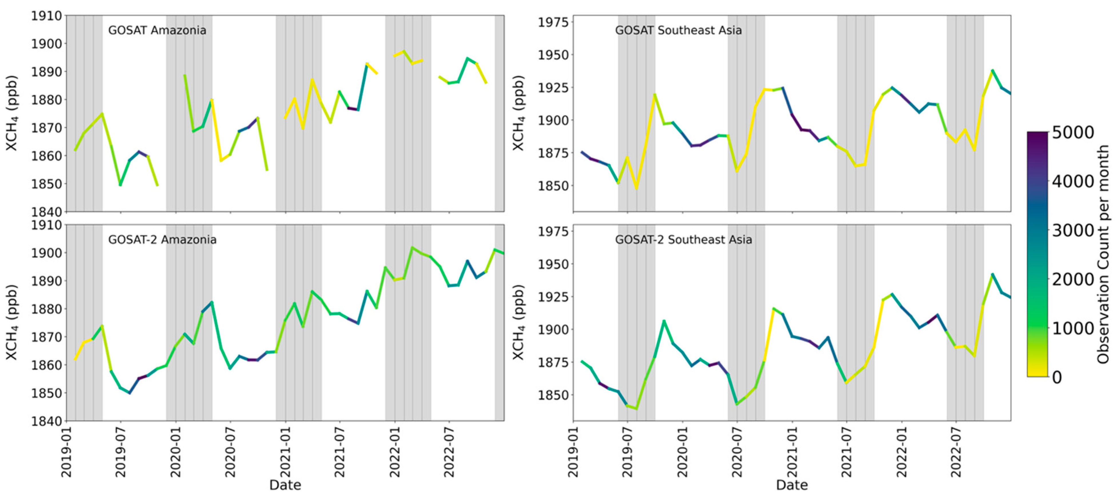
Though observations were retrieved using similar algorithms from two satellites, there can be regional inconsistencies between the products. Figure 4 presents the monthly perspective of the difference between GOSAT and GOSAT-2 XCH4 products (averaged on a 10°×10° grid). We can see that there exist considerable regional differences between the two Level 2 products, especially over Africa, Europe, and eastern Asia. GOSAT-2 XCH4 is higher over northern Africa, the Middle East, Europe, and India during most of the months (Jan- Sept). GOSAT-2 XCH4 is lower than GOSAT over Russia, China, Southeast Asia, and adjoining oceanic regions from March to September (Figure 4). Over the United States, GOSAT-2 has lower XCH4 for almost all months. These seasonally persistent differences in the XCH4 influence the estimated fluxes, as can be seen in Figure 2. We should, however, note that the differences in the two data products shown in the mean picture need not be only due to regional biases in Level 2 products, but also due to any seasonally dependent quality control filter applied to each observation. For example, over regions with seasonal cloud cover, such as monsoon Asia, filtering out observations from cloudy scenes can leave the remaining data not representative of the whole year. As an example, in Figure 7, we present the time series evolution of average XCH4 roughly over Amazonia (80-50°W; 10°S-10°N) and East Asia (80-120°E; 20-60°N). For both regions, there is a seasonal minimum concentration from June to September months. So, if observations are cleared for cloud cover, there is a chance that the majority of observations represent a slightly elevated XCH4 over East Asia than it would be in the actual case. On the contrary, the convective season over Amazonia is from December to April. Filtering observations during this season will reduce observations of peak wetland methane emissions following the inundation. For satellites having a large number of observations, such as GOSAT-2 (almost double compared to GOSAT), there will still be more observations to compensate for the filtered-out data (Figure 6). These differences become crucial when the region is poorly constrained by surface observations. For example, for almost half of the year, the east and southeast Asian and tropical African regions have significant differences in the representative XCH4 shown in Figure 4. This can be seen reflected in the difference in the flux corrections with the two sets of Level 2 products (Figure 2).
Figure 6.
The difference in the number of observations of GOSAT and GOSAT-2 in each 10° grid (GOSAT-2 – GOSAT). The country maps may not represent the actual political boundaries.
Figure 6.
The difference in the number of observations of GOSAT and GOSAT-2 in each 10° grid (GOSAT-2 – GOSAT). The country maps may not represent the actual political boundaries.
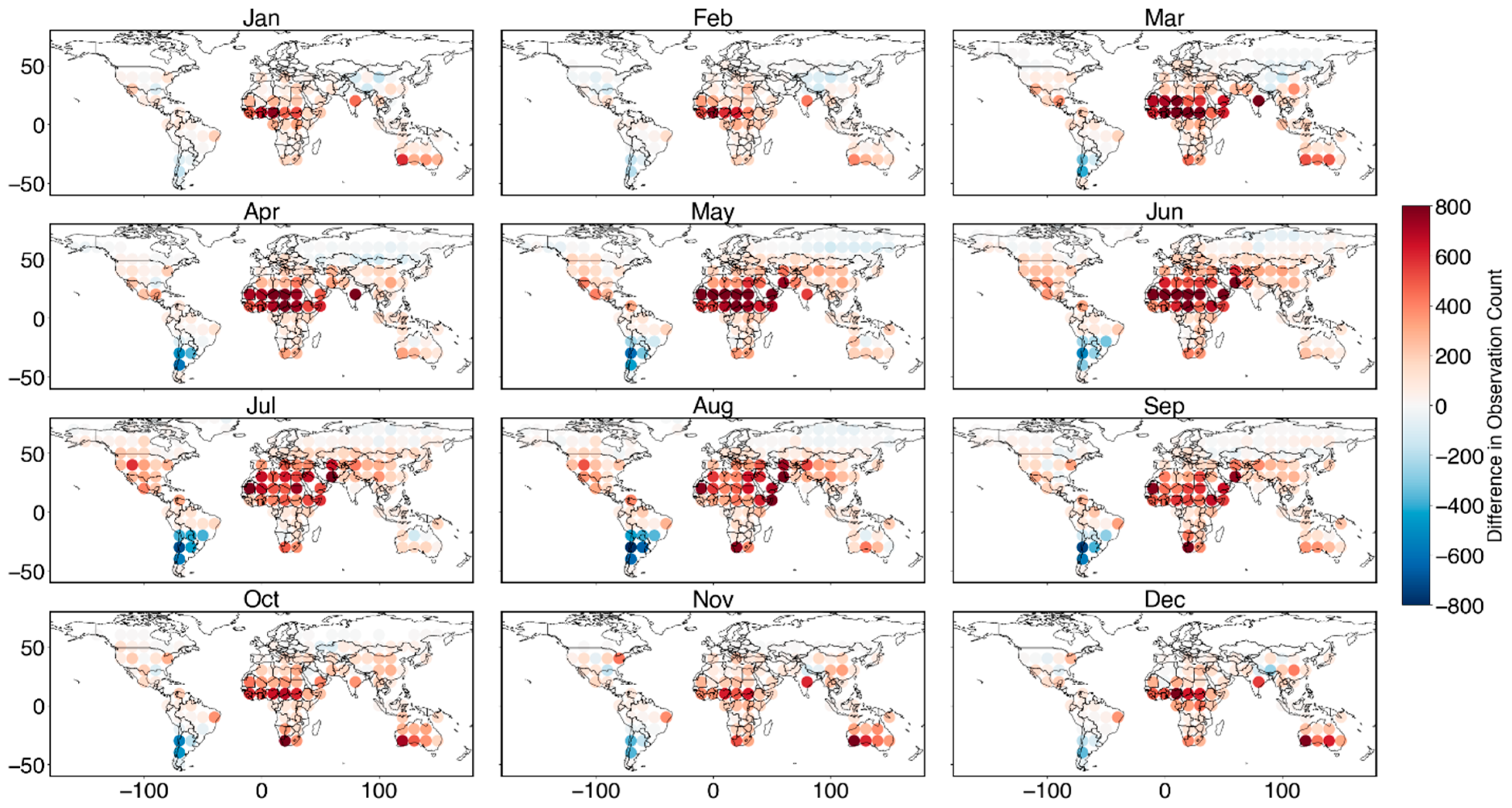
Figure 7.
Time series of monthly area-averaged XCH4 values over Amazonia and East Asia regions. The months of June to September are shaded, which means the dry season for Brazil and the wet season for East Asia.
Figure 7.
Time series of monthly area-averaged XCH4 values over Amazonia and East Asia regions. The months of June to September are shaded, which means the dry season for Brazil and the wet season for East Asia.
Yoshida et al. (2023) examined the consistency of XCO2 and XCH4 retrievals between GOSAT and GOSAT-2 and found an overall agreement between the two satellites, but pointed out the need for additional surface-based validation sites in light of the regional differences in bias between them. In their validation of GOSAT and GOSAT-2 XCH4 products with TCCON observations, they found a negative bias of -5.7 ppb around the Darwin TCCON site for GOSAT-2, but no sufficient data is available for GOSAT. A similar negative BIAS was found over Burgos for GOSAT-2, while a strong positive BIAS was found for Saga (Table 2 of Yoshida et al., 2023). In summary, though there are only a few sites for validation, their results indicate that there is likely considerable BIAS for both GOSAT and GOSAT-2 over East Asia remaining in the products. Comparatively lower emissions by GOSAT-2 inversion over the region covering Southeast Asia and Australia indicate that this is influenced by the lower GOSAT-2 XCH4 data. They have attributed the higher Xgas concentration in GOSAT-2 over Northern Africa (similar to biases in Figure 4) to the bias in the aerosol optical thickness in GOSAT-2 retrieval compared to GOSAT.
3.3.2. Regional Differences in Data Density
Comparing the data volume for composite months (Figure 6), there is apparently a lower number of GOSAT-2 observations over Northern North America, Russia, and southern South America. Apart from these regions, all other regions have a higher data count for GOSAT-2. This means that these regions have additional observational constraints by GOSAT-2, especially over regions not adequately observed by surface sites. Though there is a reduction in GOSAT-2 data over Russia, the differences in posterior emissions are not statistically significant. Instead, there are statistically significant differences in the other regions, e.g., Canada, Argentina, Chile, etc. The XCH4 over the southern part of South America, North America, and Russia is remarkably lower (Figure 4), however, the GOSAT-2 inversion allocates more emissions over southern South America and boreal North America. The higher emission over southern South America in GOSAT-2 inversions is attributable to the anomalously low number of satellite observations (Figure 6), which makes this region the most under-constrained when comparing the two inversions. In the case of boreal North America, both satellite datasets have limited observations. This makes this region yet another under-constrained area, and the model allocates more flux there. Over Africa, GOSAT-2 is biased (higher than GOSAT) and has the largest regional data volume, so that this region is normally under-constrained by the surface observation network and has larger emissions across all sectors in GOSAT-2 inversion. A major reason for the observed differences in the regionally inferred fluxes could potentially be the seasonal dependence in quality filtering of Level 2 data between these products. For example, the cloud screening of the Level 2 products can be seasonally dependent over monsoon Asia during the northern hemispheric summer. Since GOSAT has a lower data volume compared to GOSAT-2 per month (Figures S2 and S3), cloud filtering during the monsoon season increases the fraction of available observations during non-monsoon months. Considering that this is a data-sparse region as far as surface observations are concerned, this region remains under-constrained during summer. However, for the East Asian domain, the average XCH4 has a seasonal low during monsoon (Figure 7) and hence has an inherent tendency to infer higher aggregated emissions over this region. In other words, this leads to an insufficient representation of the CH4 seasonal cycle. On the other hand, GOSAT-2 has a higher number of observations to compensate for the filtered-out observations. Considering that these regions are poorly constrained by the surface networks, there is an apparent difference in the estimated fluxes.
The GOSAT and GOSAT-2 Level 2 products exhibit considerable regional differences (Figure 4) that need to be fixed. The African continent has high CH4 for GOSAT-2 from February to August, while it has lower XCH4 over and adjoining regions of East Asia from May through September. Figure 6 shows the difference in the number of observations between GOSAT and GOSAT-2 during the 2019-2022 period, counted in 10°×10° grids over the globe. The actual data count for them can be seen in Figures S2 and S3. The difference is not very significant during the northern winter months (Nov-Feb) but is apparent in the months from March to September, especially over Africa, South America, and regions of India and China. GOSAT-2 has twice as the observations per day as GOSAT and thus leaves more observations after filtering out cloudy scenes. Therefore, GOSAT-2 has higher data volume during warmer months in Africa and Southeast Asia. However, despite GOSAT-2 having more data overall, GOSAT has higher data density over southern South America. This depends on the higher sensitivity of FTS-2 onboard GOSAT-2 to abundant cosmic ray influx over the South Atlantic Anomaly of the geomagnetic field and the resultant contamination of spectra, which are filtered out during the retrieval process. From Figure 4, we can see that there are some significant regional biases from March to September over Asia, Africa, and South American regions between the observations from the two instruments. Figure 7 gives the time series of XCH4 averaged over the spatial regions represented by 80-50°W, 10°S-10°N, and 80-120°E, 0-30°N, respectively, over Amazonia and East Asian regions. We focus only on these two regions because the difference in flux corrections by the inversions using the two satellite data is sizable (Figure 2). Over East Asia, the time series has a seasonal minimum during the June to September period, or close to northern summer. Similarly, over the Amazon region, averaged XCH4 by GOSAT and GOSAT-2 shows a seasonal minimum during this season, though the cycle is not well defined. The ultimate effect of this seasonally dependent quality filtering is inadequate representation of the seasonal cycle in XCH4 data, leading to biased estimates in the fluxes, where GOSAT-2 has an advantage in East Asia due to its larger volume of data.
4. Conclusions
In this paper, for the first time, we use GOSAT-2 observations along with observations from a surface observation network for inverse estimation of sectoral methane emissions for the 2019-2022 period. We have analyzed the results of GOSAT-2 inversion together with methane emissions estimated using GOSAT observations. The objective of the study was a comparative analysis of estimated sectoral fluxes from these two inversions and their regional consistency, identifying the potential causes of any inconsistency, and noting which dataset performs better over large regions such as North America, East Asia, and Europe. Overall, the two inversions generally agree over the global sectoral emissions, while they have differences from a regional point of view. Major differences in the estimated sectoral fluxes are generally over East and Southeast Asia, Africa, and tropical South America. These regions coincide with the areas where GOSAT and GOSAT-2 have inconsistencies in the XCH4 product. GOSAT-2 tends to have lower XCH4 over East and Southeast Asia and the neighboring oceanic regions, while GOSAT-2 has higher XCH4 values over Africa, the Middle East, and India. Although validation of the sectoral optimized fluxes is difficult using independent observations, we analyze the plausible reasons for the regional differences in the total fluxes inferred by the two sets of satellite observations. Most of our independent data are from North America and Europe, and the distribution of residuals after optimization shows reduced bias than prior residuals over these two spatial domains. However, there are other regions, such as Asia, where GOSAT-2 performs better. The most valuable contribution of satellite observations in flux inversion is over such regions with sparse surface-based observation coverage. The NIES retrieval algorithm used for the two satellite Level 2 products is similar, but there are regional differences in the XCH4 data. Remaining biases in Level 2 products significantly affect flux estimates, especially in regions with limited surface network constraints. Recent studies emphasized the causes for such regional differences in XCH4 products, such as the simultaneously retrieved aerosol optical depth over, for example, the African continent, and the need for further corrections of biases in the Level 2 data. Apart from the differences in the retrieval products, quality filtering that removes data for a particular season in one product can also make a difference. We have found that the net annual emissions inferred from the satellite products can be influenced by the regional biases in the data from different sources when the region has poor coverage by the surface observations included in the inversion, as well as when surface-based total column observation sites like TCCON used for bias correction of the satellite data do not represent the region adequately. This difficulty is exacerbated if the region’s XCH4 has lower data volume due to quality filtering, which depends on seasonal cloud cover, such as monsoon Asia. From the results of the analysis in this study, we emphasize the need for establishing key observation sites in data-sparse regions such as Asia, including reference sites used for the validation of satellite observations, and ensuring sufficient data volume during cloudy seasons, especially for the utility of the combined use of satellite data from different platforms in inferring surface fluxes.
The limitations of the study include the use of non-bias-corrected GOSAT-2 data, while we used bias-corrected GOSAT data. However, we do apply a bias correction based on a surface-optimized forward model. Another point is that, for validation, we have quite a few observations in the Asian region, especially East Asia, where we found a better performance for GOSAT-2.
Supplementary Materials
The following supporting information can be downloaded at the website of this paper posted on Preprints.org.
Author Contributions
RJ conducted the inversions, analyzed the data, and prepared the initial manuscript. SM developed the model, prepared the Lagrangian simulations, and provided discussions during the preparation of the manuscript. FW and LN provided critical discussions and revised the manuscript. YY prepared the satellite Level-2 data and revised the manuscript. XL contributed several observations used in this inversion and shared constructive comments during the analysis and revision of the manuscript. TM supervised the project and the study.
Acknowledgments
We thank the Ministry of the Environment, Japan, for the financial support for the GOSAT project, under which this work was carried out. The simulations were carried out at the supercomputing facility at the National Institute for Environmental Studies, Tsukuba, Japan. The authors acknowledge the PIs and contributors related to the operations in the compilations of the Obspack CH4 dataset (obspack_ch4_1_GLOBALVIEWplus_v4.0_2021-10-14) and ICOS network. The contributions from the following people and institutions are thankfully acknowledged. A di Sarra and S. Piacentino (ENEA); A. Zahn, F. Obersteiner, H. Boenisch and T. Gehrlein (KIT/IMK); A. Desai (UofWI); A. Karion (NIST); A. Andrews, B. Baier, C. Sweeney, E. Dlugokencky, E. Hintsa, F. Moore, J. B. Miller, K. McKain and K. N. Schuldt (NOAA); A. Colomb and J. M. Pichon (OPGC); B. Scheeren and H. Chen (RUG); B. Viner (SRNL); B. Stephens (NCAR); C. Labuschagne (SAWS); C. L. Myhre, K. Tørseth and O. Hermanssen (NILU); C. E. Miller (NASA-JPL); C.-H. Lee, H. Lee, H.-Y. Kang and M.-Y. Ko (KMA); C. Plass-Duelmer, D. Kubistin, M. Schumacher and M. Lindauer (DWD); C. Gerbig (MPI-BGC); C. D. Sloop (EN); D. Jaffe (UofWA); D. Munro (NOAA-CIRES); D. Worthy (ECCC); E. Kozlova (CEDA); E. Gloor (UoL); E. Cuevas and P. P. Rivas (AEMET); E. Kort (UoM); G. Vitkova, K. Kominkova and M. V. Marek (CAS); G. Manca and P. Bergamaschi (JRC); G. Brailsford and S. Nichol (NIWA); H. Matsueda (MRI); I. Lehner, T. Biermann and M. Heliasz (LUND-CEC); I. Mammarella and P. Keronen (UHELS); J. W. Elkins (HATS); J. Müller-Williams (HPB); J. Arduini (UNIURB); J. Turnbull (GNS); J. Lee (UofME); J. P. DiGangi (NASA-LaRC); J. Hatakka, T. Laurila and T. Aalto (FMI); J. Holst and M. Mölder (LUND-NATEKO); K. Saito (JMA); K. Davis, N. Miles, S. Richardson and T. Lauvaux (PSU); L. V. Gatti (INPE); L. Emmenegger and M. Steinbacher (EMPA); L. Haszpra (RCAES); M. K. Sha and M. De Mazière (BIRA-IASB); J. M. Metzger (LACy); M. Delmotte, M. Ramonet, M. Lopez and V. Kazan (LSCE); M. L. Fischer and M. Torn (LBNL); M. Leuenberger (KUP); M. Sasakawa, T. Machida and Y. Niwa (NIES); O. Laurent (ICOS-ATC); P. Trisolino, P. Cristofanelli (CNR-ISAC); P. Krummel, R. Langenfelds and Z. Loh (CSIRO); P. Shepson (PU); P. Smith (SLU); S. C. Biraud (LBNL-ARM); S. Morimoto and S. Aoki (TU); S. O'Doherty (UNIVBRIS); S. Wofsy (HU); S. Conil (Andra); T. Schuck (IAU); V. Ivakhov (MGO); D. Goto (NIPR).
References
- Basu, S., Guerlet, S., Butz, A., Houweling, S., Hasekamp, O., Aben, I., Krummel, P., Steele, P., Langenfelds, R., Torn, M., Biraud, S., Stephens, B., Andrews, A., Worthy, D., 2013. Global CO2 fluxes estimated from GOSAT retrievals of total column CO2. Atmospheric Chemistry and Physics 13, 8695–8717. [CrossRef]
- Belikov, D.A., Maksyutov, S., Yaremchuk, A., Ganshin, A., Kaminski, T., Blessing, S., Sasakawa, M., J. Gomez-Pelaez, A., Starchenko, A., 2016. Adjoint of the global Eulerian-Lagrangian coupled atmospheric transport model (A-GELCA v1.0): Development and validation. Geoscientific Model Development 9, 749–764. [CrossRef]
- Chen, Z., Jacob, D.J., Nesser, H., Sulprizio, M.P., Lorente, A., Varon, D.J., Lu, X., Shen, L., Qu, Z., Penn, E., Yu, X., 2022. Methane emissions from China: a high-resolution inversion of TROPOMI satellite observations. Atmospheric Chemistry and Physics 22, 10809–10826. [CrossRef]
- Chevallier, F., 2007. Impact of correlated observation errors on inverted CO2 surface fluxes from OCO measurements. Geophysical Research Letters 34, 1–6. [CrossRef]
- Crippa, M., Solazzo, E., Huang, G., Guizzardi, D., Koffi, E., Muntean, M., Schieberle, C., Friedrich, R., Janssens-Maenhout, G., 2020. High resolution temporal profiles in the Emissions Database for Global Atmospheric Research. Scientific Data 7, 121. [CrossRef]
- Dlugokencky, E. J., Lan, X., Crotwell, A., Thoning, K., and Crotwell, M.: Atmospheric Methane Dry Air Mole Fractions from the NOAA ESRL Carbon Cycle Cooperative Global Air Sampling Network [dataset], ftp://aftp.cmdl.noaa.gov/data/trace_gases/ch4/flask/surface/, 2021.
- Etiope, G., Ciotoli, G., Schwietzke, S., Schoell, M., 2019. Gridded maps of geological methane emissions and their isotopic signature. Earth System Science Data 11, 1–22. [CrossRef]
- Gilbert, J.C., Lemaréchal, C., 1989. Some numerical experiments with variable-storage quasi-Newton algorithms. Mathematical Programming 45, 407–435. [CrossRef]
- Höglund-Isaksson, L., 2012. Global anthropogenic methane emissions 2005-2030: technical mitigation potentials and costs. Atmospheric Chemistry and Physics 12, 9079–9096. [CrossRef]
- ICOS RI, 2021. ICOS Atmosphere Release 2021-1 of Level 2 Greenhouse Gas Mole Fractions of CO2, CH4, N2O, CO, meteorology and 14CO2. [CrossRef]
- Janardanan, R., Maksyutov, S., Tsuruta, A., Wang, F., Tiwari, Y.K., Valsala, V., Ito, A., Yoshida, Y., Kaiser, J.W., Janssens-Maenhout, G., Arshinov, M., Sasakawa, M., Tohjima, Y., Worthy, D.E.J., Dlugokencky, E.J., Ramonet, M., Arduini, J., Lavric, J.V., Piacentino, S., Krummel, P.B., Langenfelds, R.L., Mammarella, I., Matsunaga, T., 2020. Country-Scale Analysis of Methane Emissions with a High-Resolution Inverse Model Using GOSAT and Surface Observations. Remote Sensing 12. [CrossRef]
- Janardanan, R., Maksyutov, S., Wang, F., Nayagam, L., Sahu, S.K., Mangaraj, P., Saunois, M., Lan, X., Matsunaga, T., 2024. Country-level methane emissions and their sectoral trends during 2009–2020 estimated by high-resolution inversion of GOSAT and surface observations. Environmental Research Letters 19, 034007. [CrossRef]
- Kuze, A., Suto, H., Nakajima, M., Hamazaki, T., 2009. Thermal and near infrared sensor for carbon observation Fourier-transform spectrometer on the Greenhouse Gases Observing Satellite for greenhouse gases monitoring. Applied Optics 48, 6716–6716. [CrossRef]
- Lan, X., Tans, P., Thoning, K., & NOAA Global Monitoring Laboratory, 2023. NOAA Greenhouse Gas Marine Boundary Layer Reference - CH4. [Data set]. NOAA GML. [CrossRef]
- Lan, X., K.W. Thoning, and E.J. Dlugokencky, 2022. Trends in globally-averaged CH4, N2O, and SF6 determined from NOAA Global Monitoring Laboratory measurements. Version 2024-11. [CrossRef]
- Liang, R., Zhang, Y., Chen, W., Zhang, P., Liu, J., Chen, C., Mao, H., Shen, G., Qu, Z., Chen, Z., Zhou, M., Wang, P., Parker, R.J., Boesch, H., Lorente, A., Maasakkers, J.D., Aben, I., 2023. East Asian methane emissions inferred from high-resolution inversions of GOSAT and TROPOMI observations: a comparative and evaluative analysis. Atmospheric Chemistry and Physics 23, 8039–8057. [CrossRef]
- Maksyutov, S., Oda, T., Saito, M., Janardanan, R., Belikov, D., Kaiser, J.W., Zhuravlev, R., Ganshin, A., Valsala, V.K., Andrews, A., Chmura, L., Dlugokencky, E., Haszpra, L., Langenfelds, R.L., Machida, T., Nakazawa, T., Ramonet, M., Sweeney, C., Worthy, D., 2021. Technical note: A high-resolution inverse modelling technique for estimating surface CO2 fluxes based on the NIES-TM–FLEXPART coupled transport model and its adjoint. Atmospheric Chemistry and Physics 21, 1245–1266. [CrossRef]
- Meirink, J.F., Bergamaschi, P., Krol, M.C., 2008. Four-dimensional variational data assimilation for inverse modelling of atmospheric methane emissions: Method and comparison with synthesis inversion. Atmospheric Chemistry and Physics 8, 6341–6353. [CrossRef]
- Murguia-Flores, F., Arndt, S., Ganesan, A.L., Murray-Tortarolo, G., Hornibrook, E.R.C., 2018. Soil Methanotrophy Model (MeMo v1.0): a process-based model to quantify global uptake of atmospheric methane by soil. Geoscientific Model Development 11, 2009–2032. [CrossRef]
- Nesser, H., Jacob, D. J., Maasakkers, J. D., Lorente, A., Chen, Z., Lu, X., Shen, L., Qu, Z., Sulprizio, M. P., Winter, M., Ma, S., Bloom, A. A., Worden, J. R., Stavins, R. N., and Randles, C. A., 2024. High-resolution US methane emissions inferred from an inversion of 2019 TROPOMI satellite data: contributions from individual states, urban areas, and landfills, Atmos. Chem. Phys., 24, 5069–5091. [CrossRef]
- Onogi, K., Tsutsui, J., Koide, H., Sakamoto, M., kobayashi, S., Hatsushika, H., Matsumoto, T., Yamazaki, N., Kamahori, H., Takahashi, K., Kadokura, S., Wada, K., Kato, K., Oyama, R., Ose, T., mannoji, N., Taira, R., 2007. The JRA-25 Reanalysis. Journal of the Meteorological Society of Japan 85, 369–432. [CrossRef]
- Peng, S., Lin, X., Thompson, R.L., Xi, Y., Liu, G., Hauglustaine, D., Lan, X., Poulter, B., Ramonet, M., Saunois, M., Yin, Y., Zhang, Z., Zheng, B., Ciais, P., 2022. Wetland emission and atmospheric sink changes explain methane growth in 2020. Nature 612, 477–482. [CrossRef]
- Randerson, J.T., Van der Werf, G.R., Giglio, L., Collatz, G.J., Kasibhatla, P.S., 2017. Global Fire Emissions Database, Version 4.1 (GFEDv4). [CrossRef]
- Saunois, M., Martinez, A., Poulter, B., Zhang, Z., Raymond, P., Regnier, P., Canadell, J.G., Jackson, R.B., Patra, P.K., Bousquet, P., Ciais, P., Dlugokencky, E.J., Lan, X., Allen, G.H., Bastviken, D., Beerling, D.J., Belikov, D.A., Blake, D.R., Castaldi, S., Crippa, M., Deemer, B.R., Dennison, F., Etiope, G., Gedney, N., Höglund-Isaksson, L., Holgerson, M.A., Hopcroft, P.O., Hugelius, G., Ito, A., Jain, A.K., Janardanan, R., Johnson, M.S., Kleinen, T., Krummel, P., Lauerwald, R., Li, T., Liu, X., McDonald, K.C., Melton, J.R., Mühle, J., Müller, J., Murguia-Flores, F., Niwa, Y., Noce, S., Pan, S., Parker, R.J., Peng, C., Ramonet, M., Riley, W.J., Rocher-Ros, G., Rosentreter, J.A., Sasakawa, M., Segers, A., Smith, S.J., Stanley, E.H., Thanwerdas, J., Tian, H., Tsuruta, A., Tubiello, F.N., Weber, T.S., van der Werf, G., Worthy, D.E., Xi, Y., Yoshida, Y., Zhang, W., Zheng, B., Zhu, Q., Zhu, Q., Zhuang, Q., 2025. Global Methane Budget 2000–2020. Earth System Science Data 17, 1873–147. [CrossRef]
- Saunois, M., Stavert, A.R., Poulter, B., Bousquet, P., Canadell, J.G., Jackson, R.B., Raymond, P.A., Dlugokencky, E.J., Houweling, S., Patra, P.K., Ciais, P., Arora, V.K., Bastviken, D., Bergamaschi, P., Blake, D.R., Brailsford, G., Bruhwiler, L., Carlson, K.M., Carrol, M., Castaldi, S., Chandra, N., Crevoisier, C., Crill, P.M., Covey, K., Curry, C.L., Etiope, G., Frankenberg, C., Gedney, N., Hegglin, M.I., Höglund-Isaksson, L., Hugelius, G., Ishizawa, M., Ito, A., Janssens-Maenhout, G., Jensen, K.M., Joos, F., Kleinen, T., Krummel, P.B., Langenfelds, R.L., Laruelle, G.G., Liu, L., Machida, T., Maksyutov, S., McDonald, K.C., McNorton, J., Miller, P.A., Melton, J.R., Morino, I., Müller, J., Murguia-Flores, F., Naik, V., Niwa, Y., Noce, S., O’Doherty, S., Parker, R.J., Peng, C., Peng, S., Peters, G.P., Prigent, C., Prinn, R., Ramonet, M., Regnier, P., Riley, W.J., Rosentreter, J.A., Segers, A., Simpson, I.J., Shi, H., Smith, S.J., Steele, L.P., Thornton, B.F., Tian, H., Tohjima, Y., Tubiello, F.N., Tsuruta, A., Viovy, N., Voulgarakis, A., Weber, T.S., van Weele, M., van der Werf, G.R., Weiss, R.F., Worthy, D., Wunch, D., Yin, Y., Yoshida, Y., Zhang, W., Zhang, Z., Zhao, Y., Zheng, B., Zhu, Q., Zhu, Q., Zhuang, Q., 2020. The Global Methane Budget 2000–2017. Earth System Science Data 12, 1561–1623. [CrossRef]
- Schuldt, K.N., Di Sarra, A.G., Zahn, A., Watson, A., Ankur Desai, Karion, A., Arlyn Andrews, Colomb, A., Scheeren, B., Baier, B., Viner, B., Stephens, B., Daube, B., Labuschagne, C., Myhre, C.L., Miller, C.E., Choong-Hoon Lee, Plass-Duelmer, C., Plass-Duelmer, C., Gerbig, C., Sloop, C.D., Sweeney, C., Kubistin, D., Goto, D., Jaffe, D., Munro, D., Worthy, D., Dlugokencky, E., Kozlova, E., Gloor, E., Cuevas, E., Hintsa, E., Kort, E., Obersteiner, F., Moore, F., Vitkova, G., Manca, G., Brailsford, G., Santoni, G., Haeyoung Lee, Boenisch, H., Timas, H., Matsueda, H., Kang, H.-Y., Huilin Chen, Lehner, I., Mammarella, I., Elkins, J.W., Pittman, J., Pichon, J.M., Müller-Williams, J., Jgor Arduini, Turnbull, J., Miller, J.B., Lee, J., DiGangi, J.P., Hatakka, J., Worsey, J., Holst, J., Kominkova, K., McKain, K., Saito, K., Davis, K., Tørseth, K., Haszpra, L., Gatti, L.V., Emmenegger, L., Sha, M.K., Delmotte, M., Fischer, M.L., Schumacher, M., Torn, M., Leuenberger, M., Heimann, M., Steinbacher, M., De Mazière, M., Lindauer, M., Mölder, M., Martin, M.Y., Ko, M.-Y., Heliasz, M., Marek, M.V., Ramonet, M., Lopez, M., Sasakawa, M., Miles, N., Laurent, O., Hermanssen, O., Trisolino, P., Cristofanelli, P., Krummel, P., Shepson, P., Smith, P., Rivas, P.P., Bergamaschi, P., Keronen, P., Langenfelds, R., Leppert, R., Piacentino, S., Richardson, S., Biraud, S.C., Conil, S., Morimoto, S., Aoki, S., O’Doherty, S., Wofsy, S., Nichol, S., Schuck, T., Lauvaux, T., Seifert, T., Biermann, T., Gehrlein, T., Machida, T., Laurila, T., Aalto, T., Kazan, V., Ivakhov, V., Joubert, W., Niwa, Y., Loh, Z., 2021. Multi-laboratory compilation of atmospheric carbon dioxide data for the period 1983-2020; obspack_ch4_1_GLOBALVIEWplus_v4.0_2021-10-14.
- Shen, L., Jacob, D.J., Gautam, R., Omara, M., Scarpelli, T.R., Lorente, A., Zavala-Araiza, D., Lu, X., Chen, Z., Lin, J., 2023. National quantifications of methane emissions from fuel exploitation using high resolution inversions of satellite observations. Nature Communications 14, 4948. [CrossRef]
- Suto, H., Kataoka, F., Kikuchi, N., Knuteson, R.O., Butz, A., Haun, M., Buijs, H., Shiomi, K., Imai, H., Kuze, A., 2021. Thermal and near-infrared sensor for carbon observation Fourier transform spectrometer-2 (TANSO-FTS-2) on the Greenhouse gases Observing SATellite-2 (GOSAT-2) during its first year in orbit. Atmospheric Measurement Techniques 14, 2013–2039. [CrossRef]
- Tunnicliffe, R.L., Ganesan, A.L., Parker, R.J., Boesch, H., Gedney, N., Poulter, B., Zhang, Z., Lavrič, J.V., Walter, D., Rigby, M., Henne, S., Young, D., O’Doherty, S., 2020. Quantifying sources of Brazil’s CH4 emissions between 2010 and 2018 from satellite data. Atmospheric Chemistry and Physics 20, 13041–13067. [CrossRef]
- Wang, F., Maksyutov, S., Tsuruta, A., Janardanan, R., Ito, A., Sasakawa, M., Machida, T., Morino, I., Yoshida, Y., Kaiser, J.W., Janssens-Maenhout, G., Dlugokencky, E.J., Mammarella, I., Lavric, J.V., Matsunaga, T., 2019. Methane emission estimates by the global high-resolution inverse model using national inventories. Remote Sensing 11. [CrossRef]
- Weber, T., Wiseman, N.A., Kock, A., 2019. Global ocean methane emissions dominated by shallow coastal waters. Nature Communications 10, 4584. [CrossRef]
- Welch BL (1947) The generalization of ‘Student’s’ problem when several different population variances are involved. Biometrika 34:28–35.
- Yokota, T., Yoshida, Y., Eguchi, N., Ota, Y., Tanaka, T., Watanabe, H., Maksyutov, S., 2009. Global Concentrations of CO2 and CH4 Retrieved from GOSAT: First Preliminary Results. SOLA 5, 160–163. [CrossRef]
- Yoshida, Y., Kikuchi, N., Morino, I., Uchino, O., Oshchepkov, S., Bril, A., Saeki, T., Schutgens, N., Toon, G.C., Wunch, D., Roehl, C.M., Wennberg, P.O., Griffith, D.W.T., Deutscher, N.M., Warneke, T., Notholt, J., Robinson, J., Sherlock, V., Connor, B., Rettinger, M., Sussmann, R., Ahonen, P., Heikkinen, P., Kyro, E., Mendonca, J., Strong, K., Hase, F., Dohe, S., Yokota, T., 2013. Improvement of the retrieval algorithm for GOSAT SWIR XCO2 and XCH4 and their validation using TCCON data. Atmospheric Measurement Techniques 6, 1533–1547. [CrossRef]
- Yoshida, Y., Someya, Y., Ohyama, H., Morino, I., Matsunaga, T., Deutscher, N.M., Griffith, D.W.T., Hase, F., Iraci, L.T., Kivi, R., Notholt, J., Pollard, D.F., Té, Y., Velazco, V.A., Wunch, D., 2023. Quality Evaluation of the Column-Averaged Dry Air Mole Fractions of Carbon Dioxide and Methane Observed by GOSAT and GOSAT-2. SOLA 19, 173–184. [CrossRef]
- Zhang, Z., Poulter, B., Feldman, A.F., Ying, Q., Ciais, P., Peng, S., Li, X., 2023. Recent intensification of wetland methane feedback. Nature Climate Change 13, 430–433. [CrossRef]
Figure 1.
Climatological sectoral prior fluxes used in this study (gCH4 m-2 day-1, scale different for each panel).
Figure 1.
Climatological sectoral prior fluxes used in this study (gCH4 m-2 day-1, scale different for each panel).
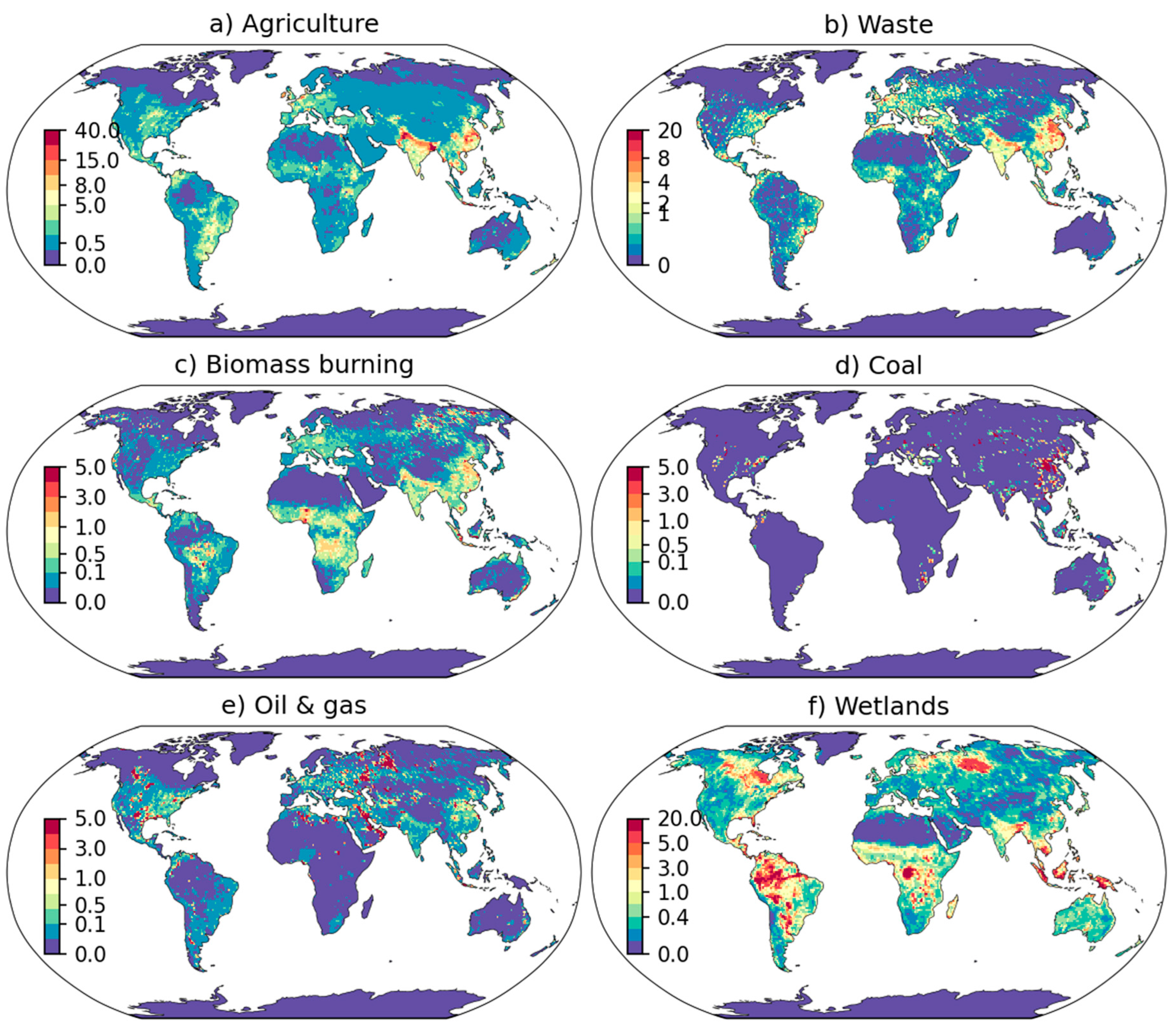
Figure 2.
The sectoral mean (2019-2022) difference in the flux corrections (gCH4 m−2 d−1) in the inversion of GOSAT and GOSAT-2 (GOSAT-2−GOSAT). The hatchings indicate regions where the mean differences are statistically significant at p < 0.01. The country maps may not represent the actual political boundaries, but only a software-dependent approximate outline.
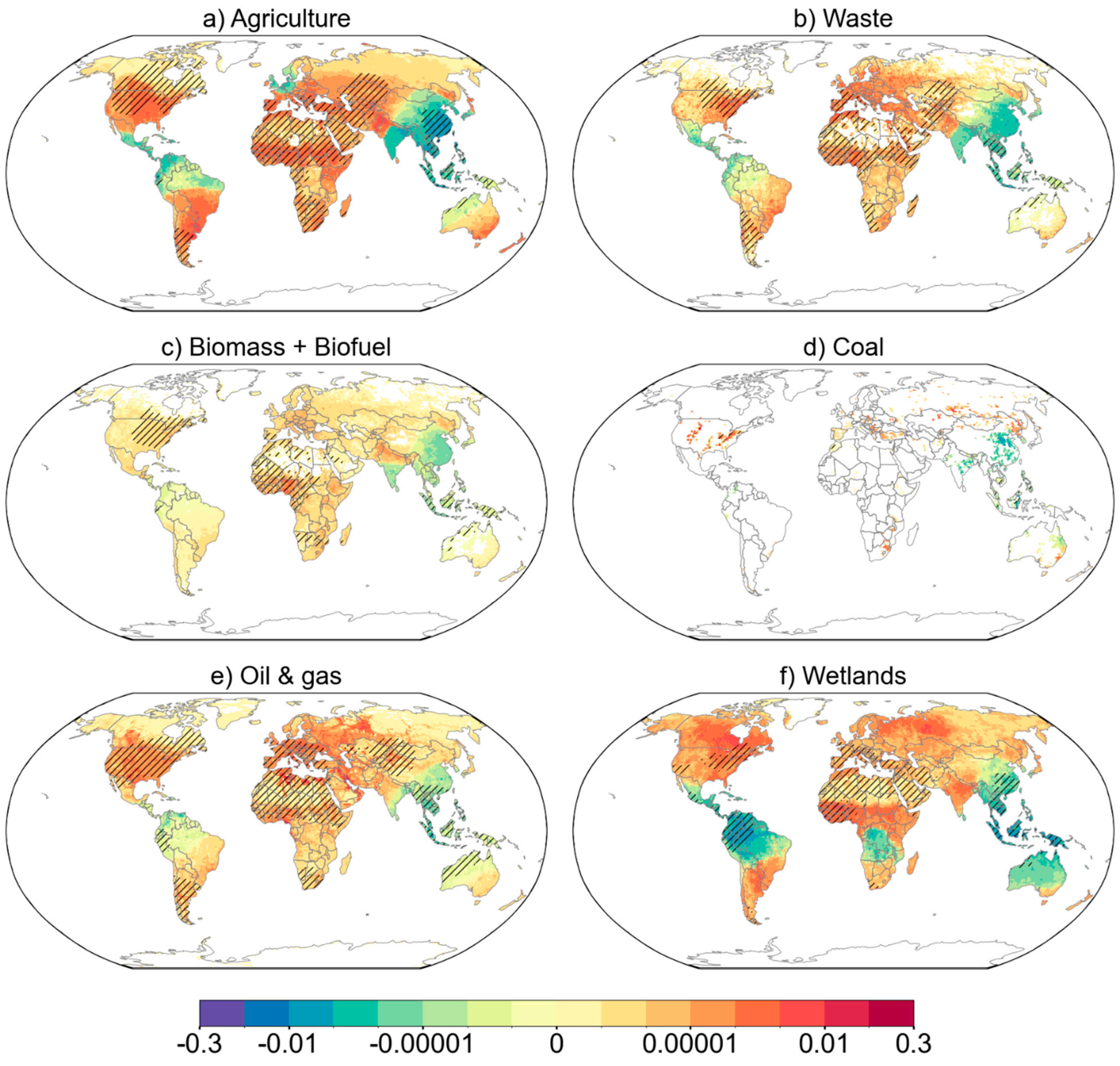
Figure 3.
The mean difference of prior and optimized forward model with GOSAT and GOSAT-2 observations gridded on a 4°×4° grid (a-d). Frequency distribution curves of prior (lighter color) and optimized (darker color) forward residuals corresponding to GOSAT (red) and GOSAT-2 (blue) inversions, for surface (e-g) and satellite (h-j) observations for three regions, North America (e, h), Europe (f, i), and Asia (g, j). The country maps may not represent the actual political boundaries.
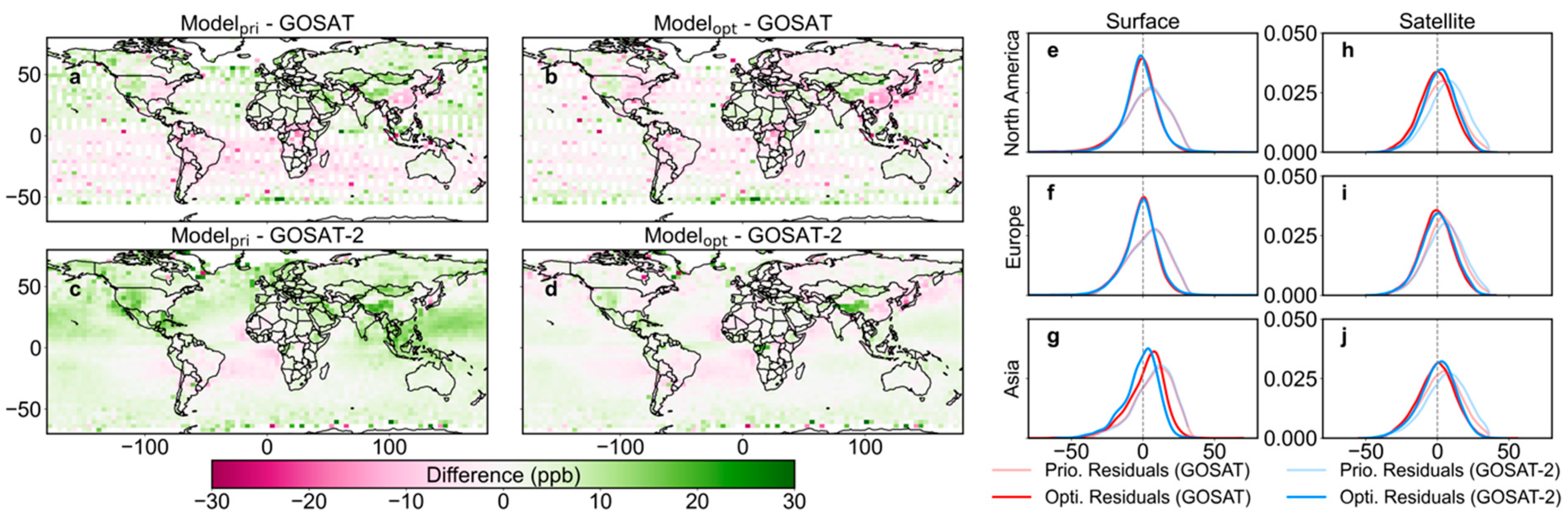
Figure 4.
The difference in mean XCH4 (GOSAT-2 – GOSAT) averaged on a 10°×10° grid for each calendar month. The country maps may not represent the actual political boundaries.
Figure 4.
The difference in mean XCH4 (GOSAT-2 – GOSAT) averaged on a 10°×10° grid for each calendar month. The country maps may not represent the actual political boundaries.
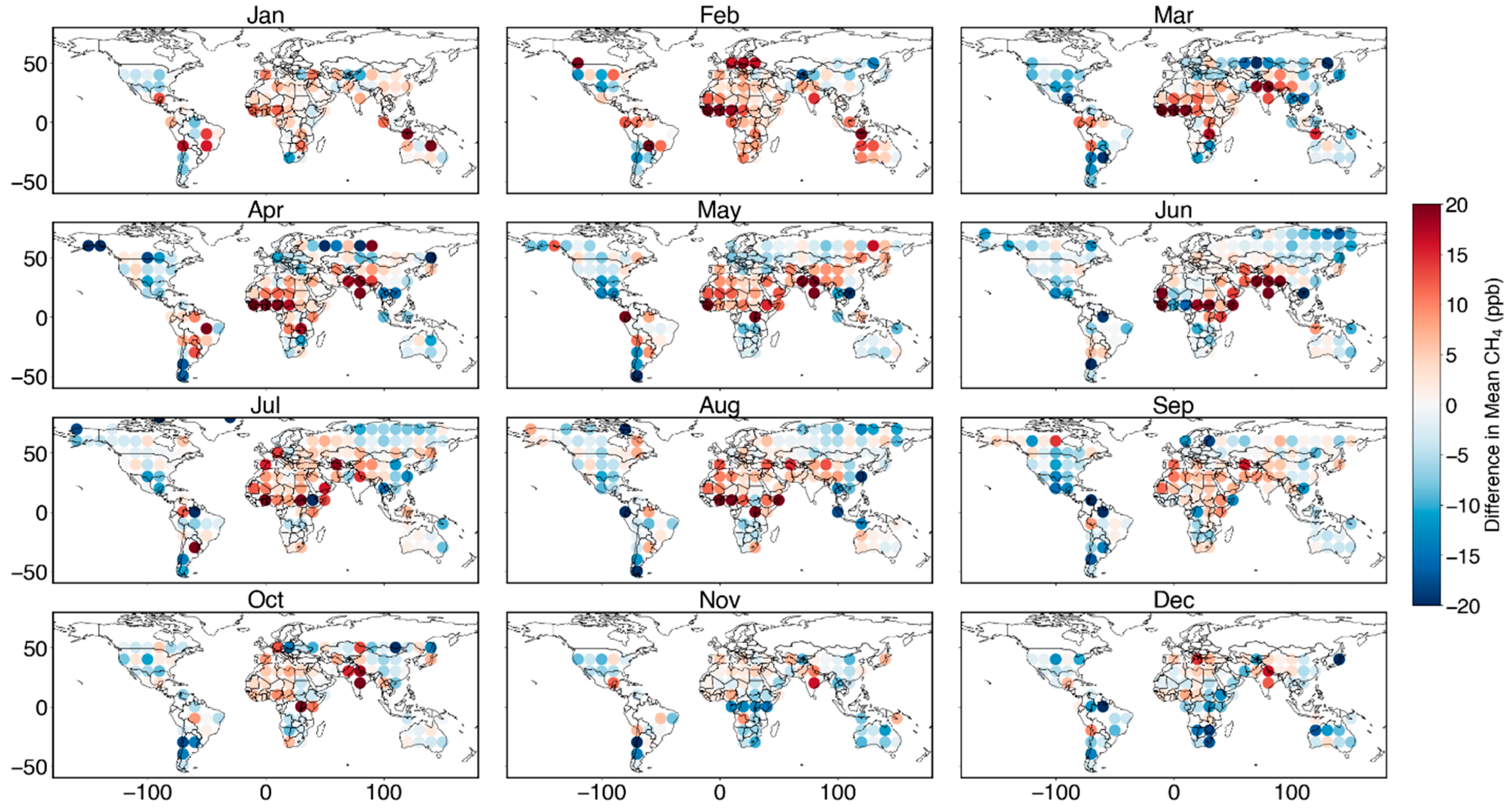
Figure 5.
Validation of the two inversions with observations that were not assimilated in the inversion step. Locations of the observation sites used in this validation are presented in a), and the kernel density estimates of the prior and posterior residuals are given in b). More details on the sites selected for validation are given in Table S2. C) comparison of the NOAA marine boundary layer reference with the latitude-wise average of optimized simulations using GOSAT and GOSAT-2 data. The sites used for averaging are a subset of the list.
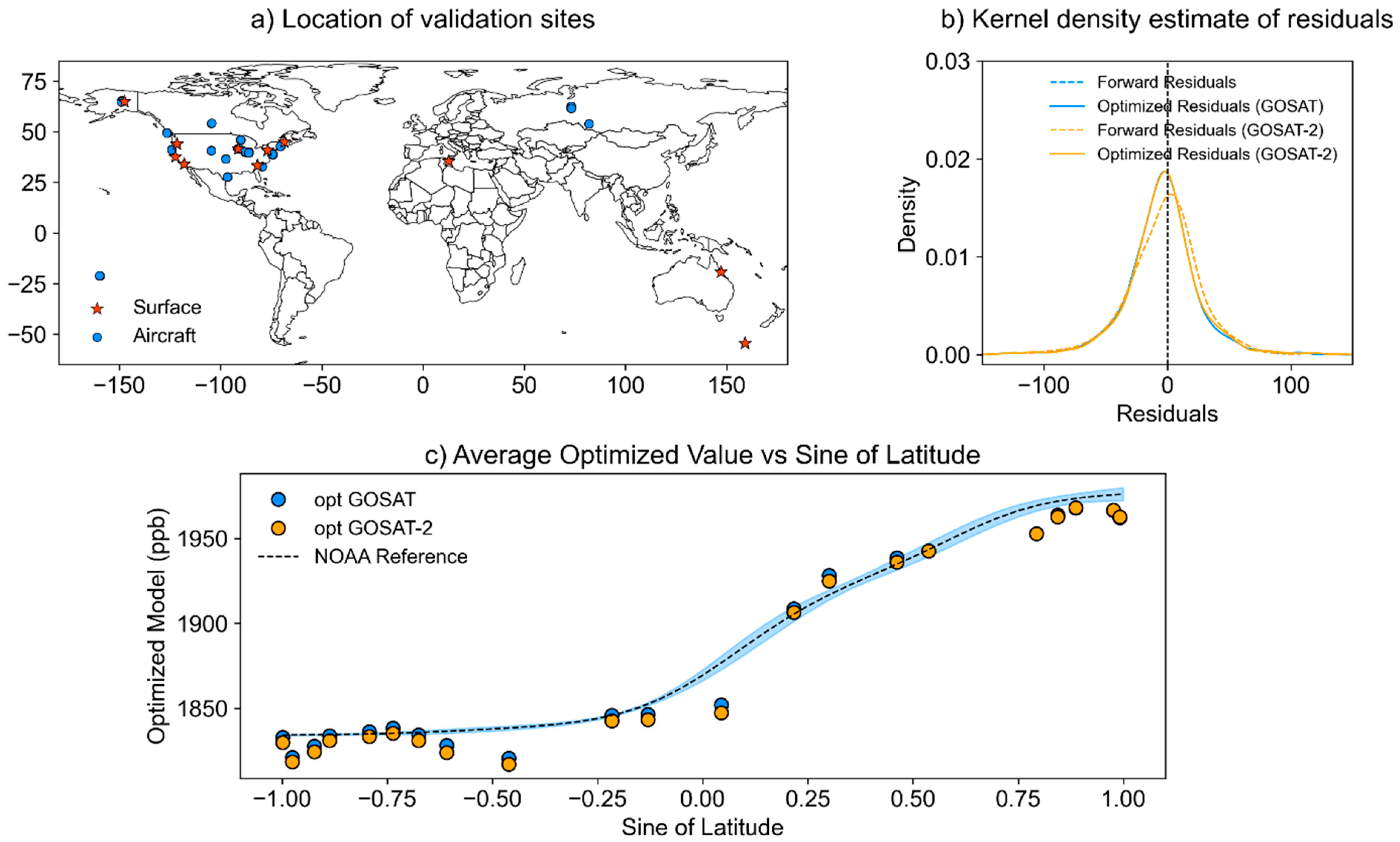

Table 1.
Global totals of sectoral emission estimates for prior, GOSAT, and GOSAT-2 inversions in units of Tg yr-1. The values are the mean for the 2019-2022 period. Sectors marked with an asterisk were not optimized.
Table 1.
Global totals of sectoral emission estimates for prior, GOSAT, and GOSAT-2 inversions in units of Tg yr-1. The values are the mean for the 2019-2022 period. Sectors marked with an asterisk were not optimized.
| Sectors | Prior | GOSAT inversion | GOSAT-2 inversion |
| Total | 615.27 | 605.20 | 601.83 |
| Agriculture | 159.85 | 156.23 | 154.72 |
| Waste | 82.34 | 80.02 | 80.28 |
| Biomass burning | 26.86 | 22.78 | 22.79 |
| Coal | 37.81 | 36.50 | 36.14 |
| Geological* | 23.02 | 23.02 | 23.02 |
| Other microbial* | 9.91 | 9.91 | 9.91 |
| Ocean* | 11.48 | 11.48 | 11.48 |
| Oil & gas | 90.02 | 83.52 | 87.79 |
| Wetlands | 173.99 | 177.84 | 171.80 |
| Soil sink* | -35.51 | -35.51 | -35.51 |
Table 2.
Comparison of country-level sectoral emissions inferred by inversion of GOSAT and GOSAT-2 data and the associated uncertainties for selected major emitting countries in units of Tg yr-1.
Table 2.
Comparison of country-level sectoral emissions inferred by inversion of GOSAT and GOSAT-2 data and the associated uncertainties for selected major emitting countries in units of Tg yr-1.
| Sectors | Agriculture | Waste | Biomass and biofuel | Coal | Oil & Gas | Wetland | ||||||
| Country | GOSAT | GOSAT-2 | GOSAT | GOSAT-2 | GOSAT | GOSAT-2 | GOSAT | GOSAT-2 | GOSAT | GOSAT-2 | GOSAT | GOSAT-2 |
| ARG | 2.34±0.25 | 2.97±0.31 | 0.52±0.01 | 0.55±0.01 | 0.11±0.00 | 0.11±0.00 | 0.00±0.00 | 0.00±0.00 | 0.44±0.01 | 0.47±0.01 | 3.58±0.15 | 3.86±0.16 |
| AUS.1 | 1.89±0.24 | 2.04±0.26 | 0.31±0.01 | 0.31±0.01 | 0.88±0.02 | 0.88±0.02 | 0.79±0.05 | 0.79±0.05 | 0.27±0.00 | 0.26±0.00 | 3.84±0.16 | 3.40±0.14 |
| BOL | 0.72±0.02 | 0.75±0.02 | 0.08±0.00 | 0.08±0.00 | 0.44±0.00 | 0.44±0.00 | 0.00±0.00 | 0.00±0.00 | 0.12±0.00 | 0.12±0.00 | 4.68±0.27 | 4.38±0.26 |
| BRA | 13.52±0.36 | 14.29±0.38 | 4.91±0.09 | 5.06±0.09 | 1.85±0.04 | 1.85±0.04 | 0.05±0.00 | 0.05±0.00 | 0.22±0.01 | 0.23±0.01 | 30.50±1.67 | 26.19±1.44 |
| CAN | 1.06±0.02 | 1.15±0.02 | 0.57±0.01 | 0.62±0.01 | 0.46±0.00 | 0.46±0.00 | 0.08±0.01 | 0.08±0.01 | 2.68±0.11 | 2.84±0.12 | 11.20±0.70 | 13.49±0.84 |
| CHN | 23.18±1.54 | 16.82±1.12 | 14.36±0.70 | 13.35±0.65 | 2.47±0.03 | 2.42±0.03 | 18.97±0.98 | 18.31±0.95 | 2.69±0.02 | 2.75±0.02 | 3.03±0.09 | 2.92±0.09 |
| COL | 1.89±0.05 | 1.80±0.05 | 0.82±0.01 | 0.80±0.01 | 0.07±0.00 | 0.07±0.00 | 0.20±0.00 | 0.20±0.00 | 0.44±0.02 | 0.43±0.02 | 6.19±0.35 | 4.71±0.27 |
| COG | 0.02±0.00 | 0.03±0.00 | 0.03±0.00 | 0.03±0.00 | 0.08±0.00 | 0.08±0.00 | 0.00±0.00 | 0.00±0.00 | 0.06±0.00 | 0.07±0.00 | 5.97±0.25 | 5.95±0.25 |
| COD | 0.30±0.00 | 0.31±0.00 | 0.64±0.02 | 0.64±0.02 | 1.35±0.04 | 1.35±0.04 | 0.00±0.00 | 0.00±0.00 | 0.02±0.00 | 0.02±0.00 | 13.59±0.80 | 13.44±0.79 |
| IND | 16.37±1.63 | 15.73±1.56 | 6.56±0.15 | 6.44±0.15 | 1.23±0.05 | 1.23±0.05 | 1.11±0.05 | 1.05±0.05 | 0.47±0.01 | 0.47±0.01 | 3.92±0.17 | 4.06±0.17 |
| IDN | 3.70±0.34 | 3.20±0.30 | 2.04±0.11 | 1.89±0.10 | 2.17±0.01 | 2.17±0.01 | 4.83±0.30 | 4.53±0.28 | 0.79±0.06 | 0.60±0.04 | 12.12±0.77 | 7.72±0.49 |
| IRQ | 0.13±0.02 | 0.14±0.03 | 0.44±0.01 | 0.46±0.01 | 0.00±0.00 | 0.00±0.00 | 0.00±0.00 | 0.00±0.00 | 6.38±0.96 | 6.91±1.04 | 0.09±0.00 | 0.10±0.00 |
| MEX | 2.67±0.05 | 2.65±0.05 | 2.48±0.03 | 2.43±0.03 | 0.21±0.00 | 0.21±0.00 | 0.01±0.01 | 0.01±0.01 | 0.29±0.02 | 0.30±0.02 | 1.35±0.05 | 1.29±0.05 |
| NGA | 1.85±0.04 | 2.25±0.05 | 1.47±0.02 | 1.57±0.02 | 0.85±0.01 | 0.90±0.01 | 0.00±0.00 | 0.00±0.00 | 2.08±0.37 | 2.86±0.51 | 1.77±0.11 | 2.09±0.13 |
| PAK | 5.34±0.37 | 5.87±0.41 | 1.30±0.03 | 1.33±0.04 | 0.32±0.01 | 0.33±0.01 | 0.03±0.00 | 0.03±0.00 | 0.53±0.03 | 0.56±0.04 | 0.16±0.01 | 0.16±0.01 |
| PER | 0.53±0.00 | 0.52±0.00 | 0.27±0.00 | 0.27±0.00 | 0.04±0.00 | 0.04±0.00 | 0.00±0.00 | 0.00±0.00 | 0.03±0.00 | 0.03±0.00 | 7.80±0.53 | 6.18±0.42 |
| RUS | 1.59±0.02 | 1.67±0.02 | 3.36±0.03 | 3.53±0.04 | 2.93±0.35 | 2.93±0.35 | 3.15±0.13 | 3.24±0.13 | 15.78±0.41 | 16.36±0.43 | 14.54±1.19 | 15.50±1.27 |
| SDN | 2.58±0.03 | 2.98±0.04 | 0.44±0.01 | 0.45±0.01 | 0.34±0.00 | 0.34±0.00 | 0.00±-0.00 | 0.00±-0.00 | 0.59±0.02 | 0.61±0.02 | 3.13±0.23 | 3.40±0.25 |
| THA | 2.50±0.49 | 2.01±0.39 | 0.95±0.03 | 0.87±0.03 | 0.13±0.03 | 0.13±0.03 | 0.01±0.00 | 0.01±0.00 | 0.12±0.01 | 0.08±0.01 | 1.10±0.08 | 0.89±0.06 |
| USA | 9.63±0.29 | 10.79±0.32 | 4.29±0.05 | 4.62±0.06 | 0.68±0.08 | 0.68±0.08 | 1.44±0.28 | 1.60±0.31 | 20.57±0.28 | 21.09±0.29 | 5.58±0.28 | 6.20±0.32 |
| VEN | 1.17±0.02 | 1.12±0.02 | 0.36±0.00 | 0.36±0.00 | 0.15±0.01 | 0.15±0.01 | 0.01±0.00 | 0.01±0.00 | 0.47±0.01 | 0.45±0.01 | 4.52±0.35 | 3.44±0.26 |
Disclaimer/Publisher’s Note: The statements, opinions and data contained in all publications are solely those of the individual author(s) and contributor(s) and not of MDPI and/or the editor(s). MDPI and/or the editor(s) disclaim responsibility for any injury to people or property resulting from any ideas, methods, instructions or products referred to in the content. |
© 2025 by the authors. Licensee MDPI, Basel, Switzerland. This article is an open access article distributed under the terms and conditions of the Creative Commons Attribution (CC BY) license (http://creativecommons.org/licenses/by/4.0/).
Copyright: This open access article is published under a Creative Commons CC BY 4.0 license, which permit the free download, distribution, and reuse, provided that the author and preprint are cited in any reuse.


