
Submitted:
07 July 2025
Posted:
09 July 2025
You are already at the latest version
Abstract
Accurate segmentation of kidney microstructures in whole slide images (WSIs) is essential for diagnosing and monitoring renal diseases. This study proposes an end-to-end instance segmentation pipeline for detecting glomeruli and blood vessels in hematoxylin and eosin (H\&E) stained kidney tissue. Using Slicing Aided Hyper Inference (SAHI), we apply a tiling-based approach to manage the high resolution and scale of WSIs and evaluate the performance of two recent segmentation models, YOLOv11 and YOLOv12. Additionally, we evaluate the effect of different tile overlap ratios on segmentation quality and inference efficiency, identifying configurations that balance object continuity with computational cost. To address object fragmentation at tile boundaries, we introduce an Enhanced Syncretic Mask Merging algorithm, incorporating morphological and spatial constraints. Hyperparameters of the merging algorithm are optimized using Particle Swarm Optimization (PSO), targeting vessel and glomerulus specific performance. The optimization process identified parameters that most influenced performance, particularly for vessel segmentation, where fine structure posed challenges and edge fragmentation was less common. Experimental results demonstrate a 48\% average precision improvement in glomerulus segmentation with a maximum improvement of 17\% for blood vessels. The proposed framework effectively balances segmentation accuracy and inference efficiency, supporting high-throughput histopathology analysis and contributing to the Vasculature Common Coordinate Framework (VCCF) and Human Reference Atlas (HRA).
Keywords:
instance segmentation
; kidney whole slide images
; slicing aided hyper inference
; syncretic mask merging
; particle swarm optimization
1. Introduction
The kidney is a vital organ liable for preserving systemic homeostasis by regulating blood filtration, fluid balance, electrolyte composition and acid base status. Around one million functional units called nephrons are contained within each kidney, with each nephron beginning at the glomerulus, a specialized network of capillaries that serves as the primary blood filtration site. Roughly one fifth of cardiac output flows through the kidneys’ finely tuned vasculature to ensure appropriate renal blood flow and glomerulus filtration rate [1]. Blood vessels in the kidneys, including arterioles, capillaries and venules are critical for delivering blood to the glomeruli, modulating filtration and supporting metabolic demands. The glomerulus capillaries, in particular, enable size and charge selective filtration of plasma, allowing waste products to be removed while retaining essential proteins and cells. Damage to this vascular network or the glomerule filtration barrier can lead to proteinuria, chronic kidney disease or end stage renal disease [2]. Additionally, vascular dysfunction, fibrosis or microvascular rarefaction within the kidney contribute to progression of disease and loss of function [1]. = Given the central role of vascular health and glomerulus integrity in kidney physiology and systemic health, accurate assessment is critical for diagnosing and monitoring kidney diseases. Kidney biopsies, imaged at high resolution, remain the standard for such assessments. Modern whole slide imaging (WSI) technology enables the digitization of entire biopsy slides at subcellular resolution, producing images that may span gigapixels in size. However, traditional image analysis methods such as manual inspection, thresholding and morphological operations are labor intensive, time consuming and often lack reproducibility across different imaging conditions or pathological states [3]. AI models inspired by biological neural mechanisms, such as convolutional neural networks (CNN), have reached remarkable accuracy in segmentation tasks. However, processing entire image requires significant memory, storage and processing power and remains an open research challenge.
To manage this, a common approach is tiling, where the large image is divided into smaller, overlapping or non overlapping tiles that can fit within the memory constraints. Models are trained on these tiles and during inference, predictions from individual tiles are aggregated to produce the final segmentation or detection map of the entire WSI. An example of such a technique is Slicing Aided Hyper Inference (SAHI), an open source framework proposed by [4]. Once predictions are made on individual image tiles or slices, a postprocessing step is required to remove duplicate detections and consolidate outputs into a coherent result for the entire whole slide image. Traditional Non Maximum Suppression (NMS) [5] is the most widely used method for this purpose. To improve upon the limitations of traditional Non Maximum Suppression (NMS) in handling fragmented or partially detected objects, Syncretic NMS [6] was introduced to merge correlated neighboring boxes into more complete bounding boxes, improving contextual accuracy. However, applying standard Syncretic NMS to SAHI based tiling in whole slide image analysis introduces new challenges. When tiles do not overlap, there is no shared IoU between adjacent tile detections, which makes it difficult for Syncretic NMS to identify and merge corresponding bounding boxes. Even in overlapping tile configurations, irregularly shaped objects frequently result in low IoU values between detections on neighboring tiles, leading to potential misclassifications or failure to merge correctly. Moreover, standard Syncretic NMS is not optimized for the low density, spatially variable and morphologically complex structures commonly encountered in histopathology. To overcome these limitations, an enhanced mask merging method has been proposed, with optimized mask merging criteria and refinement steps. The selection of optimal parameters for this algorithm is recognized as an NP-hard problem and an optimization strategy is discussed to identify the best performing configuration for our case.
This study presents methods for improving instance segmentation in gigantic whole slide images. The performance of two recently released instance segmentation models, YOLOv11 and YOLOv12, is evaluated for this task, with both models trained using a tiling approach. Additionally, the impact of tile overlap on segmentation quality is investigated to identify an optimal range. To enhance postprocessing and address the challenges of fragmented objects, a modified version of Syncretic NMS is proposed to better consolidate partial detections across tiles. Furthermore, the parameter tuning problem is explored as an optimization challenge to identify optimal configurations. The entire framework is trained and validated on a publicly available dataset specifically developed for segmentation models targeting microvascular structures in renal tissue, ensuring real world applicability.
This research contributes to:
- Latest YOLOv11 and YOLOv12 instance segmentation models are comparatively evaluated and SAHI’s tiling inference is validated on large medical slides.
- Evaluates the impact of tile overlap that improves edge region segmentation accuracy while maintaining efficient inference.
- An enhanced syncretic mask merging technique is introduced, designed to enable seamless and precise reconstruction of objects fragmented by tile borders.
- Demonstrates the complete pipeline, including parameter optimization, on a public dataset designed for evaluating microvascular structures models in H&E stained human kidney slides.
The paper proceeds with the following sections: Section 2 reviews related works including small object detection challenges, SAHI tiling, original Syncretic NMS and most recent YOLO segmentation models with loss function considerations. Section 3 outlines the architecture and implementation of selected YOLO models, introduces the proposed modified algorithm and outlines the optimization method for parameter tuning. Section 4 describes the experimental configuration, including dataset, model training strategy, tiling layout and evaluation metrics. Section 5 presents the outcomes of our experiments. Lastly, Section 6 is devoted to concluding the study and suggesting potential avenues for future research.
2. Related Works
Small object detection is a specialized subfield within computer vision and object detection, concerned with accurately detecting and localizing objects that occupy relatively small regions within an image or video frame [7]. Unlike conventional object detection, which often focuses on medium or large objects, small object detection requires overcoming unique challenges related to scale, resolution and dataset bias [8]. The importance of small object detection has grown in recent years due to its relevance across a wide array of real world applications, ranging from surveillance and autonomous driving to robotics, environmental monitoring and industrial automation. In medical imaging, object detection helps by enabling the identification of anomalies such as tumors, lesions and microvascular changes within organs. Accurate detection is essential for early diagnosis, effective treatment planning and tracking disease progression [9]. However, the task remains inherently challenging due to a combination of anatomical complexity, resolution constraints and the limited visibility. Receptive fields in convolutional neural networks often fail to capture enough context for accurate detection. Small objects occupy very few pixels with minimal details for feature extraction which are further increased by class imbalance in training datasets [10]. While approaches such as tiling and improved training strategies have shown promise, a clear gap remains in the literature regarding kidney tissue segmentation, particularly in the development of postprocessing techniques for de-duplication and merging of fragmented detections, defining a challenge targeted in the present work.
Instance segmentation differs from traditional object detection or image classification, as it requires precise pixel level delineation of each individual object instance [11]. Unlike object detection, where bounding box localization is sufficient, instance segmentation relies on subsequent semantic segmentation steps [12]. Traditional Non Maximum Suppression (NMS) [5] is a widely used postprocessing algorithm, designed to remove redundant bounding boxes by selecting those with the highest confidence scores while suppressing overlapping boxes. However, traditional NMS was originally formulated for object detection tasks and is suboptimal when applied to instance segmentation [13]. In particular, traditional NMS focuses on maximizing box overlap with the ground truth, but it does not guarantee that the entire object is fully enclosed by the final selected bounding box. In instance segmentation, this poses a significant issue: if parts of an object lie outside of the final bounding box, those parts cannot be included in subsequent pixel level segmentation, degrading segmentation accuracy. Therefore, additional postprocessing steps are often necessary to ensure that the full extent of each object is captured, enabling accurate pixel level segmentation in instance segmentation tasks [14]. In this paper, we aim to address this challenge by proposing a method that complements traditional NMS with a refinement stage to better preserve object completeness.
2.1. YOLO Loss Function
The You Only Look Once (YOLO) model approaches object detection by treating it as a single step prediction problem. Instead of breaking the process into multiple stages, it uses one neural network pass to directly predict object locations and categories all at once. The YOLO algorithm starts by splitting the input image into a grid made up of equal sized cells. Each of these cells is responsible for detecting objects whose centers fall within it. For each grid cell, the model generates B bounding boxes, each accompanied by a confidence score that reflects both the probability of object presence and the accuracy of its predicted location. Additionally, each cell predicts the probabilities that the detected object belongs to specific classes [15]. However, achieving accurate predictions requires a carefully designed loss function that guides the model during training.
The total loss function in YOLO combines four main components: localization loss, object confidence loss, no-object confidence loss and classification loss [15]:
Each component plays a distinct role and small object detection presents unique challenges for all of them:
- Localization loss (): Localization errors affect small objects excessively, challenging accurate spatial prediction.
- Confidence loss (): Weak features make it harder to assign high confidence to small object predictions.
- No-object loss (): Over penalization in background regions can suppress valid small object detections.
- Classification loss (): Small objects often lack strong class specific features, leading to misclassifications.
The classification loss, for example, penalizes the difference between the predicted and actual class probabilities for grid cells that contain an object:
- : indicator function, 1 if an object is detected in cell i.
- : ground truth probability of class c for grid cell i.
- : predicted probability of class c.
To improve box regression stability, advanced loss formulations are used in place of traditional mean squared error (MSE). Overlap loss is extended in CIoU [16] through additional geometric constraints and distance penalties, improving alignment between predicted and ground truth. It incorporates both the distance between bounding box centers and the similarity of aspect ratios into the following formulation:
- : intersection over union between predicted and ground truth boxes.
- d: the length between centroids of bounding boxes measured by Euclidean distance .
- c: the diagonal span of the union of the predicted and ground truth boxes.
- v: a term measuring the consistency of aspect ratios.
- : a dynamic weighting factor for v.
This approach produces stable gradients even when the predicted and ground truth boxes have no overlap. In such cases, standard IoU based losses yield zero gradients, impeding learning, whereas CIoU continues to guide the model toward better localization and alignment across tiled image segments [16] and is extended further in proposed postprocessing algorithm.
2.2. Slicing Aided Hyper Inference
Slicing Aided Hyper Inference [4] is a framework poposed to improve object detection in large images by simply dividing them into overlapping tiles or patches. The patch dimensions are determined by two primary parameters: slice_height and slice_width, which define the vertical and horizontal size of each patch, respectively. To ensure continuity between neighboring patches, an overlap is introduced. The degree of overlap is controlled by the parameters overlap_height_ratio and overlap_width_ratio, both of which are ratios between 0 and 1 that determine the percentage of overlap between adjacent patches.
The patch generation process can be described formally with the following algorithm:
| Algorithm 1: Slicing Aided Hyper Inference (SAHI) |
|
- : Processed image I height and width.
- : Height and width of each patch (tile).
- : Vertical and horizontal overlap proportion.
- : Vertical and horizontal strides between patches.
- : Minimum confidence threshold for keeping detections.
- : IoU limit for detecting overlapping.
- P: A single image patch extracted from the input image I.
- d: List of raw detections on patch P
- : A postprocessing de-duplication function like NMS
- : Filtered detections on patch P after applying G.
- D: List of all detections for image I.
Each element in D corresponds to a detection result from a patch and typically includes bounding box coordinates, confidence score, class label and a binary mask representing the shape of the detected object.
The effectiveness of the SAHI pipeline depends on the choice of slicing parameters , which typically require empirical tuning. No universal defaults exist and optimal values vary depending on dataset characteristics and object scale. After collecting all detections in D, a final merging step is necessary to reconcile overlapping or redundant predictions across patches. This is particularly important when objects are located near tile boundaries or are fragmented across multiple slices, potentially up to four different patches. In such cases, standard overlap based merging approaches may fail, which is common with irregularly shaped objects or when there is no tile overlapping [4]. These limitations may result in missed detections, duplicate predictions or fragmented segmentation. Although patch wise inference has become common, the literature lacks postprocessing techniques specifically designed to handle this challenge in tiled instance segmentation tasks. In this research, a dedicated method is introduced to perform the final merging of detections with improved accuracy and robustness, particularly for edge aligned and fragmented objects.
2.3. Syncretic NMS
To address limitations of traditional instance segmentation de-duplication methods, Syncretic NMS [6] was introduced as an enhanced merging NMS algorithm specifically designed for instance segmentation. The algorithm builds upon traditional NMS but incorporates an additional merging step that explicitly considers neighboring bounding boxes. After performing a standard NMS pass to obtain an initial set of bounding boxes D, Syncretic NMS iteratively examines neighboring bounding boxes of each box in D and evaluates their correlation. If the correlation between a neighboring box and a candidate box exceeds a threshold , the boxes are merged to form a larger box that fully encloses both regions. The merged bounding box coordinates are computed as the extreme values of the combined set of boxes: the minimum , maximum , maximum and minimum among all merged boxes.
| Algorithm 2:Original Syncretic-NMS Merging Algorithm |
|
- B: List of input candidate boxes .
- S: List of confidence scores associated with each box in B.
- : IoU limit to decide on the overlapping box candidates.
- : Correlation limit used for decision whether to merge two boxes should be merged.
- : Box with the maximum score .
- A: Temporary list of boxes to be merged, including and its correlated neighbors.
- : Function that returns a new box by combining all boxes in A using:
- D: Resulting set of merged boxes.
Syncretic NMS represents a step forward over traditional NMS by incorporating a merging mechanism that evaluates the correlation between neighboring bounding boxes, allowing for the combination of highly related detections. This results in more complete bounding boxes, which is especially beneficial for instance segmentation tasks. However, Syncretic NMS was not originally developed for tiled inference scenarios or SAHI based pipelines. To address this, a modified algorithm tailored for merging fragmented detections in tiled image analysis is introduced. The proposed method, which builds upon the Syncretic framework, is specifically designed for instance segmentation tasks and is detailed in Section 3.
3. Methods
3.1. Implementation and Training of YOLO Models
Recent YOLO versions have introduced architectural enhancements aimed at improving instance segmentation performance. The YOLOv11 model [17] integrates a transformer based backbone to enhance global spatial understanding and selectively applies attention mechanisms to enrich feature representations without incurring additional computational cost. Building upon this, the YOLOv12 model [18] introduces area attention and Residual Efficient Layer Aggregation Networks (RELAN). RELAN enhances the model’s ability to capture spatial dependencies by dividing feature maps into regions and aggregating information from multiple network layers using residual connections and a redesigned feature aggregation strategy. This mechanism is implemented via lightweight A2C2f blocks, which aggregate contextual information from adjacent regions using efficient 2D attention and depthwise separable convolutions. This enables more effective fusion of low level details and high level semantic features, resulting in improved object detection accuracy and more stable training dynamics.
The PyTorch YOLO segmentation models provided by Ultralytics [19] were utilized. These models use convolutional neural networks as the backbone for feature extraction. Lightweight components such as C3k2 blocks promote feature reuse, while C2PSA attention modules enhance the model’s focus on spatially relevant information. Additionally, multi scale segmentation heads are employed to refine mask predictions across varying object sizes by leveraging feature maps from different network depths [17]. This multi scale strategy enables effective detection of both small and large structures, as each head specializes in a specific scale of object representation. Such approaches have been shown to significantly improve segmentation performance in real time models like YOLO-MS [20].
Two YOLO-based instance segmentation models are explored in this study: the compact YOLOv11s-seg and the more recent YOLOv12s-seg. The YOLOv11s-seg model comprises 355 layers and approximately 10.1 million parameters (35.6 GFLOPs). Both models were trained on tiled inputs derived from a kidney histology dataset for 100 epochs using Automatic Mixed Precision (AMP). AMP accelerates training by utilizing FP16 operations where safe, while retaining FP32 precision where necessary, thereby reducing memory usage and improving training speed, beneficial for high resolution images. The AdamW optimizer was used, with learning rate and momentum parameters automatically tuned via Ultralytics’ built in hyperparameter search. Similarly, the YOLOv12s-seg model, consisting of 533 layers, 9.75 million parameters and 33.6 GFLOPs [18], was trained under the same regime. Both models were trained and evaluated under identical conditions to secure balanced evaluation.
3.2. Proposed Enhanced Syncretic Mask Merging
To overcome the limitations of traditional bounding box based merging in large scale image inference, the Syncretic NMS framework is extended with a modified merging criteria and morphological postprocessing procedure. Proposed method is specifically tailored for tiled instance segmentation and introduces object level reasoning that preserves the continuity of biological structures across tile borders. As a result, fragmentation and duplication artifacts, commonly observed in tiled inference settings, are effectively addressed.
The enhanced Syncretic strategy generalizes prior approaches by applying merging to binary object masks rather than bounding boxes, using a flexible mergeability predicate and additional morphological operations to resolve overlapping or fragmented instances across tiles. Instead of relying solely on IoU, the algorithm leverages contour level spatial clustering and appearance based feature similarity to identify object fragments spanning tile boundaries. Specifically, border objects are detected and clustered using a spatial proximity radius, with merging decisions guided by contour similarity , feature similarity , bounding box IoU and semantic label agreement . The resulting clusters are fused into unified masks via logical union, followed by contour simplification and polygon extraction. A final morphological refinement stage applies gap closing, hole filling and one pass dilation to improve continuity and recover thin or clipped regions. Figure 1 illustrates mask merging process, showing how fragmented instances are accurately grouped and reconstructed across adjacent tiles.
The algorithm operates in two major stages: (1) object level clustering based on spatial, semantic and feature similarity and (2) morphological refinement. First, all detected instances are converted from local tile coordinates into a unified global space. Objects near tile boundaries are designated as merge candidates and grouped into a global candidate set. Merging proceeds iteratively: at each step, the highest confidence object is selected as a seed and neighboring candidates are evaluated for compatibility using a mergeability predicate . This predicate considers semantic class consistency, contour proximity, feature vector similarity and geometric overlap. Compatible objects are grouped into a cluster and merged via the operator , producing a unified mask instance.
| Algorithm 3:Enhanced Syncretic Merging Algorithm |
|
where:
- : The i-th tile in the WSI, with local detections, masks, scores and class labels.
- : Tile upper left corner.
- n: Total number of tiles in the WSI.
- : List of border objects in tile , whose bounding boxes or masks lie within border_threshold_px of any tile edge.
- : List of all objects near border .
- B: Working candidate list built from unmatched objects in at the start of each iteration.
- : Object in B with the highest confidence in the current iteration.
- A: Merge group initialized with and extended with nearby compatible objects.
- : A candidate object in B evaluated for merging with .
- : New merged object resulting from applying .
- G: Final list of merged global objects to be returned.
- border_threshold_px: Pixel threshold defining how close an object must be to a tile edge to be considered a border object.
- search_radius: Maximum spatial distance (in pixels) within which object pairs are considered for merging.
The mergeability predicate is evaluated using the following criteria:
where:
The functions defining the mergeability predicate and their thresholds are as follows: in Equation (6) captures contour based spatial proximity and is constrained by the distance contour_proximity_thresh (); in Equation (5), measures cosine similarity of features that are over the cosine_sim_thresh (); , representing the IoU between bounding boxes, which must meet the minimum threshold bbox_iou_thresh (); in Equation (8), a binary indicator ensuring semantic class consistency [23].
In the equations (5)–(8), and denote the sets of foreground pixels (or sampled points) from the masks of objects and , respectively. and represent their corresponding feature vectors, which may be derived from intermediate neural network embeddings. and are the sets of contour or boundary points extracted from the object masks. The represents the confidence score of object predicted. The operator refers to the Euclidean norm and denotes the cardinality of a set. The dot product is used in computing cosine similarity and the intersection and union operators in correspond to standard binary mask operations.
The merge operator refines the final set G by combining all objects in a cluster A through the logical union of their masks, simplifying shapes via polygon approximation and applying a morphological postprocessing stage to enhance coherence and correct under segmentation. The merged object retains the semantic class and has its features and bounding box recomputed. Algorithm 4 outlines the morphological refinement procedure applied to the merged object set G to enhance segmentation coherence.
| Algorithm 4:Morphological Refinement |
|
The parameters and control the dilation of small objects during morphological refinement, improving boundary quality in the final set G. Parameter defines the structuring element size for class specific morphological operations such as closing. Parameter adjusts the accuracy of polygonal contour approximation, balancing detail and simplicity.
In terms of computational complexity, the Enhanced Mask Merge algorithm scales as , where N is the number of border objects, k is the average number of nearby candidates considered for merging and d is the dimensionality of the feature vectors used in similarity evaluation. These feature vectors encode appearance or shape characteristics and are used to compute cosine similarity between objects. In contrast, the Syncretic NMS algorithm does not rely on feature vectors and instead performs pairwise comparisons based solely on geometric overlap (IoU) and confidence scores. As a result, its worst case complexity is , since each box may be compared with all others. While Syncretic NMS is simpler and effective for small scale scenarios, its quadratic growth becomes computationally expensive as N increases. Enhanced Mask Merge, by leveraging spatial locality and feature based filtering, offers a scalable alternative for large scale instance merging tasks.
3.3. Hyperparameter Optimization via PSO
Metaheuristic algorithms are flexible methods used to solve complex optimization problems, especially when traditional techniques are too slow or ineffective. These algorithms are well suited for tackling challenges that involve nonlinear, high dimensional, or irregular search spaces. Particle Swarm Optimization (PSO) [24] is one such method that uses a population of candidate solutions, known as particles, which move through the search space by adjusting their positions based on both their own previous performance and the best known positions found by the group. This iterative process helps the swarm gradually converge toward an optimal or near optimal solution. The [25] package is a Python implementation of the PSO algorithm that supports custom objective functions and custom search spaces.
The proposed Enhanced Syncretic Mask Merging algorithm introduces a range of tunable hyperparameters that govern morphological smoothing, spatial proximity thresholds, shape similarity and feature level coherence. These parameters guide object refinement and cross tile merging, as such, finding optimal values is a non trivial task, as the search space is high dimensional and exhibits strong interactions between variables. This is approached as an NP-hard optimization problem and solved using a black box method. The optimization objective is to maximize the macro averaged score across all object classes. The coefficient is defined as:
This metric balances over segmentation (which reduces precision) and under segmentation (which reduces recall), making it ideal for tuning instance segmentation algorithms on imbalanced datasets. Our instance segmentation task includes two semantically distinct structures: blood vessels, which are thin and elongated and glomeruli, which are more circular, compact and significantly less frequent (approximately 50:1 ratio). To account for these differences, class specific hyperparameter ranges are introduced for key morphological and clustering operations. All parameter bounds listed in Table 1 are selected empirically based on visual inspection and performance profiling.
This approach enables efficient exploration of the parameter space, ensuring comparable performance across diverse object morphologies and class imbalances.
4. Experimental Setup
The dataset used in our work is derived from whole slide images of PAS stained human kidney tissue, with resolutions from 8,704 × 13,824 to 17,408 × 44,544 pixels, representing entire histological slides. It is prepared for the HuBMAP - Hacking the Human Vasculature Kaggle competition [26]. Slides represent healthy kidney tissue with a focus on microvascular structures. The training dataset is composed of image tiles originally extracted from 14 WSIs at 40 times magnification, corresponding to a physical area of approximately m.. These tiles are categorized into three subsets: Dataset 1 (expert reviewed annotations), Dataset 2 (sparser annotations) and Dataset 3 (unannotated tiles). While Datasets 1 and 2 originate from 5 donor slides and include polygonal masks for blood vessels, glomeruli and uncertain regions, Dataset 3 is intended for semi supervised learning and lacks annotations and demographic metadata [27].
For the training of both YOLOv11 and YOLOv12 models, a total of 6,606 images were compiled from Datasets 1 and 2, along with 1,800 self annotated tiles sourced from Dataset 3. The data was split into training, validation and test sets as follows: 5575 images (84%) for training, 685 images (10%) for validation and 346 images (5%) for testing. Each image was resized to 640×640 pixels and augmented by applying horizontal and vertical flips with a 50% probability each, resulting in three variants per original image. The tissue samples include sections from distinct anatomical regions of the kidney: renal cortex, renal medulla and renal papilla. This segmentation task not only supports basic biological mapping but also enables downstream applications like modeling blood flow, tissue oxygenation and cellular organization. Figure 2 illustrates the dataset structure, showing a full kidney whole slide image and a representative annotated tile extracted for model training.
In analysis, SAHI values in the range from 0 to 0.15 (0-15%) were explored, using increments of 0.025 (2.5%), to evaluate overlap impact on detection continuity across slice boundaries. Due to computational resource constraints, inference was performed on cropped regions of 3072×3072 pixels extracted from the original whole slide images. These regions were subsequently divided into overlapping tiles of 512×512 pixels, which were passed through the inference pipeline and postprocessing step and finally compared against the available ground truth annotations. For evaluation of the proposed segmentation pipeline, standard performance metrics commonly used in medical image analysis were computed: accuracy, precision, recall and the F1 score. These metrics quantify the quality of object detection and mask merging and are widely adopted for benchmarking segmentation and classification systems [28]. Segmentation performance is evaluated using standard metrics based on instance level matching and results are compared with ground truth annotations. The following notation is used: (correct positives), (incorrect positives) and (incorrect negatives). The term (correct negatives) is not used in this context, as it is not defined in instance segmentation tasks, where the number of true negative object instances or regions without objects and without predictions, cannot be meaningfully quantified.
The evaluation metrics are computed as follows:
To summarize performance across different overlap thresholds and IoU match criteria, the metric is computed. The is defined as:
where and in our experiments. All predictions included in this evaluation were filtered using a confidence threshold of 50% for both blood vessels and glomeruli. Due to computational resource constraints, a subset of 15 images was selected for evaluation, each composed of a 6×6 grid of tiles, to ensure representative variability across tissue structures and donors. Each tile measured pixels at 40× magnification, corresponding to a physical area of approximately m.
To identify optimal hyperparameter configurations for instance segmentation, PSO tuning is employed over a defined search space of empirically selected parameter ranges (Table 1). The Python library is used for PSO implementation, configuring a swarm of 30 particles and running for 30 iterations per cycle.. An inertia weight of 0.5 is used to balance exploration and exploitation, while cognitive and social coefficients are both set to 2.0 to guide particles toward local and global optima. The objective function maximizes the macro averaged across both classes, using instance level ground truth annotations and standard detection metrics (Accuracy, Precision, Recall and F1). This setup enables efficient exploration of the parameter space while ensuring generalization across morphological variations.
5. Experimental Results and Discussion
To assess the proposed training strategy and model architectures evaluation was conducted across multiple training epochs and inference settings. Loss components for both models consistently decreased across epochs, with no signs of overfitting observed. In the inference phase, both models successfully integrated Slicing Aided Hyper Inference (SAHI), enabling dense and overlapping tile aggregation across high resolution whole slide images. This approach allowed for precise instance segmentation while maintaining computational efficiency on large scale histology data. Table 2 presents a comparative evaluation of instance segmentation performance between YOLOv11s-seg and YOLOv12s-seg across key kidney tissue structures.
Both models achieved high segmentation performance for glomerulus, with precision and recall consistently above 88%. Blood vessel segmentation was more variable due to the finer and more diffuse structure of vascular elements. However, YOLOv11s-seg maintained a higher F1 score overall, making it more balanced in performance across both classes.
As shown in Table 3, YOLOv11s-seg was considerably more efficient, with lower GPU memory usage and faster epoch and inference times. This is particularly important in whole slide image workflows, where inference must be both accurate and fast. The reduced GPU footprint of YOLOv11s-seg also enhances its applicability in clinical or resource limited deployment environments. Given the strong segmentation performance, compact architecture and superior computational efficiency, YOLOv11s-seg was selected for downstream tasks, including framework validation and segmentation based postprocessing.
To support the quantitative results for YOLOv11s-seg, key training diagnostics and qualitative outputs are included. Figure 3 shows the Mask F1 score curve and the Mask Precision Recall (PR) curve for YOLOv11s-seg. The F1 curve tracks the harmonic mean of mask precision and recall throughout training. The PR curve visualizes the trade off between precision and recall at varying confidence thresholds, with class specific and aggregate performance shown. Glomerular segmentation demonstrates particularly strong separation, while blood vessel performance is slightly more variable. Figure 4 presents a representative validation example. The left panel shows ground truth masks for glomeruli and blood vessels overlaid on a histology tile, while the right panel displays YOLOv11s-seg’s predicted masks for the same region. Qualitatively, the model captures the boundaries and structure of glomeruli accurately, with reasonable performance on finer vascular elements.
Despite the architectural enhancements in YOLOv12s-seg, such as A2C2f blocks and deeper layer integration, the model underperformed YOLOv11s-seg in both segmentation quality and computational efficiency. Specifically, YOLOv11s-seg achieved higher mask mAP@0.5 (0.623 vs. 0.585) and overall better balance of precision and recall across key object classes. While glomerular segmentation performance remained strong in both models, YOLOv11s-seg showed slightly higher overall mAP and more consistent recall. The YOLOv12 model also incurred greater computational cost, with significantly slower inference ( 2×) and deeper network complexity. Moreover, YOLOv12s-seg required over 70% more training time and 47% more GPU memory, while offering no clear benefit in segmentation accuracy. Clearly, the additional complexity of YOLOv12s-seg does not translate into improved performance in this histological context and simpler CNN based models like YOLOv11s-seg remain more reliable for resource constrained biomedical segmentation tasks.
The impact of tile overlap ratio on segmentation performance was evaluated. Experiments were conducted using varying overlap ratios ranging from 0% to 15% in steps of 2.5%. Performance was assessed using the metric, computed as the mean F1 score across IoU thresholds 0.5–0.9 compared with ground truth. Figure 5 illustrates how segmentation quality, measured via , changes with increasing overlap. The performance improves steadily up to an overlap of approximately 7.5%, after which it plateaus or slightly declines. This suggests moderate overlap helped in restoring instance structures across tiles. As expected, inference time per image increases with larger overlaps due to redundant tile processing. Figure 5 shows a near linear increase in average runtime from 140 to over 210 seconds per image as the overlap increases from 7.5% to 15%. Based on the results, the optimal overlap ratio was found to be approximately 7.5%.
Figure 6 presents F1 scores across all IoU thresholds and overlap ratios for both blood vessels and glomeruli. These plots highlight how stricter IoU thresholds affect the precision/recall tradeoff differently across tissue types, with blood vessels showing more pronounced performance variations due to their elongated and fragmented morphology. Figure 7 shows the variation in segmentation metrics at IoU = 0.5 for both tissue types, highlighting the effect of overlap ratio on detection performance.
Figure 8 illustrates the impact of tile overlap on segmentation quality. The no-overlap result shows fragmented and incomplete segmentation’s, especially at tile boundaries, while the overlap result yields more continuous and accurate detections. As seen in the figure, the central glomerulus (red) on the left has lost its upper left corner due to tile boundary truncation. This demonstrates that moderate overlap improves prediction quality and also suggests that further postprocessing is necessary to consolidate segments across tiles, motivating our proposed enhanced mask merging method.
Based on these findings, an overlap ratio in the range of 5–7.5% is recommended for most use cases, as this range offers a favorable balance between segmentation accuracy and inference time. Overlaps within this range consistently improved object continuity across tile boundaries without introducing significant computational overhead for large scale whole slide image processing. To further refine the segmentation results, postprocessing optimization was conducted using a tile overlap of 7.5%. Table 4 presents the best performing hyperparameter configurations, both overall and separately for each class, as determined by peak score. The values listed in Table 4 represent the PSO optimized parameters used in the algorithm, with rounded values shown for implementation and original outputs provided in parentheses for reference.
The results show that glomeruli segmentation achieved near optimal performance with minimal missed instances, while vessel detection remained more challenging due to under segmentation and fragmentation. The optimized morphological kernel sizes fall within the lower end of their respective ranges, suggesting that moderate morphological closing is generally effective. Polygon approximation parameters (epsilon) support preserving shape detail, with vessels favoring higher values than glomeruli. Clustering thresholds reflect the fragmentary nature of instance predictions: low bbox_iou_thresh values (0.12–0.21) allow for permissive spatial merging, while moderate cosine_sim_thresh values maintain conservative shape agreement. Specifically, a low bbox_iou_thresh value (0.12) allows for permissive spatial merging of partially overlapping vessel fragments, compensating for breakage across tile boundaries. At the same time, a relatively high cosine_sim_thresh (0.91) ensures that only geometrically similar fragments are merged, thus guarding against the erroneous fusion of unrelated vessels. The contour_proximity_thresh values indicate that a spatial clustering radius in the 45–56 pixel range is effective. Importantly, all optimized parameters remained within the empirically defined hyperparameter bounds (Table 1), validating the suitability of the selected search space.
Figure 9 illustrates the convergence of F1 scores during PSO optimization (left) and the relative influence of each hyperparameter on macro F1 as determined by standardized linear regression (right). Regression analysis revealed that dilation_kernel, dilation_percentile and cosine_similarity had the strongest negative influence on macro . In contrast, parameters such as morphological_kernel (glomerulus), epsilon (glomerulus) and IoU_threshold showed minimal impact within the tested range. The convergence plot illustrates how PSO explored the parameter space, with many suboptimal trials and a gradual improvement toward high performing configurations. The sensitivity analysis and convergence behavior observed in this study not only validate the effectiveness of our optimization strategy but also highlight the practical application of the proposed postprocessing algorithm. By identifying a small subset of hyperparameters with high impact, future tuning efforts can be confidently prioritized around these parameters.
Additionally, qualitative and quantitative evaluations were performed using the best scoring image from each class. Figure 10 presents side by side comparisons between predicted and ground truth instance segmentation’s for the top performing image in each class.
Metrics are summarized in Table 5, including detection counts and evaluation metrics. Ground truth and predicted instance counts are reported separately, while derived metrics such as precision, recall and F1 score were computed against the reference annotations. The results demonstrate fitness of the proposed merging and cleaning algorithm. Glomerulus segmentation achieved perfect agreement with the ground truth in the best performing image, whereas blood vessel segmentation, although highly accurate, exhibited slightly lower performance due to the greater structural complexity and fragmentary nature of vascular objects.
Finally, Table 6 summarizes the average and maximum improvements (denoted as ) in segmentation performance metrics when comparing the proposed optimized pipeline against the baseline predictions. The results demonstrate that the postprocessing strategy consistently enhances segmentation accuracy. Notably, glomerulus detection benefited the most, with an average improvement of 35.7% and recall by 8.2%. While vessel segmentation achieved a moderate average precision gain of 8.15%, recall decreased slightly by 0.58%, suggesting improved boundary definition at the cost of missing some true positives. As most vessels were centrally located within tiles, the merging strategy primarily enhanced boundary alignment rather than correcting edge cut artifacts. In contrast, glomeruli more frequently spanned tile borders and thus benefited more substantially from overlap aware reconstruction. Overall, the strategy was most beneficial for glomeruli, where mask overlap resolution had a higher effect. Nonetheless, the optimized pipeline significantly boosts overall segmentation quality, supporting its applicability for complex histological instance segmentation.
A direct comparison with standard NMS or Syncretic-NMS approaches was not included, as these methods are not directly applicable to overleaped tiling pipelines and don’t include morphological postprocessing. Similarly, full resolution inference on high resolution images was excluded from comparative evaluation, since the underlying models were trained exclusively on smaller tiles extracted from whole slide images and are not optimized for global context. Instead, this work addresses the gap identified in the literature regarding tile level postprocessing under overlap and fragmentation, offering a reproducible and optimized solution. By exposing the interaction between tiling strategies, spatial overlap and postprocessing thresholds, the proposed approach aims to inform and guide future segmentation efforts in histopathology and other domains requiring high resolution instance level precision.
6. Conclusions
A complete instance segmentation pipeline for kidney histology is proposed, focusing on detecting glomeruli and blood vessels in whole slide images. The approach builds on YOLOv11 and YOLOv12 models, whose comparative performance is evaluated in this work. To improve detection continuity across tile boundaries, the overlap_ratio parameter was varied from 0 to 0.15. An overlap in the range of 5–7.5% was found to offer an effective balance between segmentation accuracy and inference efficiency.
The core contribution lies in the development of an Enhanced Syncretic Mask Merging algorithm, coupled with a postprocessing refinement step. This method directly addresses object fragmentation along tile borders by enforcing morphological, spatial and semantic consistency, resulting in improved object continuity and segmentation quality. To optimize algorithm hyperparameters, particle swarm optimization was employed over a 9-dimensional search space covering both class specific and shared parameters. Results showed that vessel segmentation was more sensitive to hyperparameter tuning, particularly to dilation_kernel, dilation_percentile and cosine_sim_thresh, while glomerulus segmentation remained strong across broader parameter ranges. This increased sensitivity is attributed to the smaller, elongated and irregular shapes of vascular structures. Consequently, future tuning efforts should prioritize vessel specific parameters to better capture their fine grained morphology.
Overall, the proposed method improved segmentation precision for larger glomeruli by an average of 48%, while vessel segmentation showed a more modest average precision gain of 8.15% reaching as high as 17%, likely due to most vessels being centrally located within tiles. These results highlight the effectiveness of proposed enhanced mask merging in segmenting structurally diverse tissue components. Future work should explore additional instance segmentation models beyond YOLO, as well as adaptive overlap strategies to further enhance boundary performance while reducing inference cost. Expanding the parameter search space or employing alternative optimization algorithms may also yield more robust tuning. Ultimately, this work contributes to an adaptable segmentation framework for large scale medical imaging, particularly suited to identifying microvascular structures in kidney tissue, directly supporting the Vasculature Common Coordinate Framework (VCCF) and the Human Reference Atlas (HRA).
Author Contributions
Conceptualization, M.M. and M.M; methodology, software, validation, formal analysis, investigation, resources, data curation, writing—original draft preparation, visualization, and project administration, M.M.; writing—review and editing, supervision, and funding acquisition, M.M. All authors have read and agreed to the published version of the manuscript.
Funding
This research was supported by the Science Fund of the Republic of Serbia, Grant No. 7502, Intelligent Multi-Agent Control and Optimization applied to Green Buildings and Environmental Monitoring Drone Swarms - ECOSwarm.
Data Availability Statement
The dataset used in this study is publicly available and was obtained from the HuBMAP: Hacking the Human Vasculature competition on Kaggle, accessible at: https://www.kaggle.com/competitions/hubmap-hacking-the-human-vasculature/data (accessed on 5 July 2025). The dataset is open source and available for research use. Refer to the competition rules for full eligibility details. The YOLO models were implemented using the open-source Ultralytics YOLO repository (version 8.0.0), available at: https://github.com/ultralytics/ultralytics (accessed on 5 July 2025). The repository is licensed under the GNU Affero General Public License v3.0 (AGPL-3.0). No proprietary or restricted data or software were used in this study.
Data Availability Statement
The dataset used in this study is publicly available and was obtained from the HuBMAP: Hacking the Human Vasculature competition on Kaggle, accessible at: https://www.kaggle.com/competitions/hubmap-hacking-the-human-vasculature/data (accessed on 5 July 2025). The dataset is open source and available for research use. Refer to the competition rules for full eligibility details. The YOLO models were implemented using the open-source Ultralytics YOLO repository (version 8.3.159), available at: https://github.com/ultralytics/ultralytics (accessed on 5 July 2025), and licensed under the GNU Affero General Public License v3.0 (AGPL-3.0). Supervision (version 0.25.1), a utility library for computer vision workflows, is available at: https://github.com/roboflow/supervision (accessed on 5 July 2025), and is licensed under the MIT License. Roboflow Inference (version 0.51.0), a toolkit for deploying computer vision models across devices and environments, is available at: https://github.com/roboflow/inference (accessed on 5 July 2025), and is also licensed under the MIT License. PySwarms, a research toolkit for Particle Swarm Optimization (PSO) in Python (version 1.3.0), is available at: https://github.com/ljvmiranda921/pyswarms (accessed on 5 July 2025), and is licensed under the MIT License. No proprietary or restricted data or software were used in this study.
Conflicts of Interest
The authors declare no conflicts of interest. The funders had no role in the design of the study; in the collection, analysis, or interpretation of data; in the writing of the manuscript; or in the decision to publish the results.
Abbreviations
The following abbreviations are used in this manuscript:
| AMP | Automatic Mixed Precision |
| CIoU | Complete Intersection over Union |
| CN | Correct Negative |
| CNN | Convolutional Neural Network |
| CP | Correct Positives |
| FLOPs | Floating Point Operations |
| GFLOPs | Giga Floating Point Operations per Second |
| GPU | Graphics Processing Unit |
| GT | Ground Truth |
| HRA | Human Reference Atlas |
| IN | Incorrect Negative |
| IP | Incorrect Positive |
| IoU | Intersection over Union |
| MSE | Mean Squared Error |
| NMM | Non-Mask Merge |
| NMS | Non-Maximum Suppression |
| PR | Precision Recall |
| PSO | Particle Swarm Optimization |
| RELAN | Residual Efficient Layer Aggregation Network |
| SAHI | Slicing Aided Hyper Inference |
| TP | True Positive |
| VCCF | Vasculature Common Coordinate Framework |
| WSI | Whole Slide Image |
| YOLO | You Only Look Once |
| mAP | Mean Average Precision |
| mAP50 | Mean Average Precision at 50% IoU |
References
- Krishnan, S.; Suarez-Martinez, A.D.; Bagher, P.; Gonzalez, A.; Liu, R.; Murfee, W.L.; Mohandas, R. Microvascular dysfunction and kidney disease: Challenges and opportunities? Microcirculation 2021, 28, e12661. [Google Scholar] [CrossRef] [PubMed]
- Semenikhina, M.; Mathew, R.O.; Barakat, M.; Van Beusecum, J.P.; Ilatovskaya, D.V.; Palygin, O. Blood pressure management strategies and podocyte health. American journal of hypertension 2025, 38, 85–96. [Google Scholar] [CrossRef] [PubMed]
- Kaur, G.; Garg, M.; Gupta, S.; Juneja, S.; Rashid, J.; Gupta, D.; Shah, A.; Shaikh, A. Automatic Identification of Glomerular in Whole-Slide Images Using a Modified UNet Model, 2023.
- Akyon, F.C.; Altinuc, S.O.; Temizel, A. Slicing Aided Hyper Inference and Fine-tuning for Small Object Detection. 2022 IEEE International Conference on Image Processing (ICIP) 2022, pp. 966–970. [CrossRef]
- Hosang, J.; Benenson, R.; Schiele, B. Learning non-maximum suppression. In Proceedings of the Proceedings of the IEEE conference on computer vision and pattern recognition, 2017, pp. 4507–4515.
- Chu, J.; Zhang, Y.; Li, S.; Leng, L.; Miao, J. Syncretic-NMS: A merging non-maximum suppression algorithm for instance segmentation. IEEE Access 2020, 8, 114705–114714. [Google Scholar] [CrossRef]
- Wei, W.; Cheng, Y.; He, J.; Zhu, X. A review of small object detection based on deep learning. Neural Computing and Applications 2024, 36, 6283–6303. [Google Scholar] [CrossRef]
- Wang, X.; Wang, A.; Yi, J.; Song, Y.; Chehri, A. Small object detection based on deep learning for remote sensing: A comprehensive review. Remote Sensing 2023, 15, 3265. [Google Scholar] [CrossRef]
- Juszczak, F.; Arnould, T.; Declèves, A.E. The role of mitochondrial sirtuins (sirt3, sirt4 and sirt5) in renal cell metabolism: Implication for kidney diseases. International Journal of Molecular Sciences 2024, 25, 6936. [Google Scholar] [CrossRef] [PubMed]
- Liu, K.; Fu, Z.; Jin, S.; Chen, Z.; Zhou, F.; Jiang, R.; Chen, Y.; Ye, J. ESOD: Efficient Small Object Detection on High-Resolution Images. IEEE Transactions on Image Processing 2024. [Google Scholar] [CrossRef] [PubMed]
- Sharma, R.; Saqib, M.; Lin, C.T.; Blumenstein, M. A survey on object instance segmentation. SN Computer Science 2022, 3, 499. [Google Scholar] [CrossRef]
- Wang, X.; Zhang, R.; Shen, C.; Kong, T.; Li, L. Solo: A simple framework for instance segmentation. IEEE transactions on pattern analysis and machine intelligence 2021, 44, 8587–8601. [Google Scholar] [CrossRef] [PubMed]
- Wang, X.; Zhang, R.; Kong, T.; Li, L.; Shen, C. Solov2: Dynamic and fast instance segmentation. Advances in Neural information processing systems 2020, 33, 17721–17732. [Google Scholar]
- Yang, Y.; Luo, W.; Tian, X. Hybrid two-stage cascade for instance segmentation of overlapping objects. Pattern Analysis and Applications 2023, 26, 957–967. [Google Scholar] [CrossRef]
- Redmon, J.; Divvala, S.; Girshick, R.; Farhadi, A. You only look once: Unified, real-time object detection. In Proceedings of the Proceedings of the IEEE conference on computer vision and pattern recognition, 2016, pp. 779–788.
- Zheng, Z.; Wang, P.; Ren, D.; Liu, W.; Ye, R.; Hu, Q.; Zuo, W. Enhancing geometric factors in model learning and inference for object detection and instance segmentation. IEEE transactions on cybernetics 2021, 52, 8574–8586. [Google Scholar] [CrossRef] [PubMed]
- Khanam, R.; Hussain, M. Yolov11: An overview of the key architectural enhancements. arXiv preprint arXiv:2410.17725 2024. arXiv:2410.17725 2024.
- Tian, Y.; Ye, Q.; Doermann, D. Yolov12: Attention-centric real-time object detectors. arXiv preprint arXiv:2502.12524 2025. arXiv:2502.12524 2025.
- Jocher, G.; Qiu, J.; Chaurasia, A. Ultralytics YOLO, 2023.
- Chen, Y.; Yuan, X.; Wu, R.; Wang, J.; Hou, Q.; Cheng, M. YOLO-MS: Rethinking multi-scale representation learning for real-time object detection. arXiv 2023. arXiv preprint arXiv:2308.05480 2023. arXiv:2308.05480 2023.
- Dokmanic, I.; Parhizkar, R.; Ranieri, J.; Vetterli, M. Euclidean distance matrices: essential theory, algorithms, and applications. IEEE Signal Processing Magazine 2015, 32, 12–30. [Google Scholar] [CrossRef]
- Lehal, M.S. Comparison of cosine, Euclidean distance and Jaccard distance. Int J Sci Res Sci, Eng Technol (IJSRSET) 2017, 3, 1376–1381. [Google Scholar]
- Thapliyal, S.; Kumar, N. Fusion of heuristics and cosine similarity measures: introducing HCSTA for image segmentation via multilevel thresholding. International Journal of System Assurance Engineering and Management 2025, pp. 1–54.
- Eberhart, R.; Kennedy, J. A new optimizer using particle swarm theory. In Proceedings of the MHS’95. Proceedings of the sixth international symposium on micro machine and human science. Ieee, 1995, pp. 39–43.
- Miranda, L.J.V. PySwarms, a research-toolkit for Particle Swarm Optimization in Python. Journal of Open Source Software 2018, 3. [Google Scholar] [CrossRef]
- Human BioMolecular Atlas Program (HuBMAP). HuBMAP - Hacking the Human Vasculature. https://www.kaggle.com/competitions/hubmap-hacking-the-human-vasculature, 2023. Kaggle competition to segment microvascular structures in human kidney tissue. Accessed: 2025-06-17.
- Hu, F.; Deng, R.; Bao, S.; Yang, H.; Huo, Y. Multi-scale Multi-site Renal Microvascular Structures Segmentation for Whole Slide Imaging in Renal Pathology. arXiv preprint arXiv:2308.05782 2023. arXiv:2308.05782 2023.
- Hossin, M.; Sulaiman, M.N. A review on evaluation metrics for data classification evaluations. International journal of data mining & knowledge management process 2015, 5, 1.
Figure 1.
Illustration of the Mask Merging Operations. Two distinct merge operations are shown: (1) the top region merges objects and across tiles T1 and T2 into ; and (2) the lower right region merges three objects—, and —spanning the shared corner of tiles T2, T3, T5 and T6 into . Merged objects are product of function .

Figure 2.
Example of dataset structure. Left: Low resolution overview of a PAS stained WSI. Right: A representative tile extracted from the WSI, showing annotated microvascular structures.
Figure 2.
Example of dataset structure. Left: Low resolution overview of a PAS stained WSI. Right: A representative tile extracted from the WSI, showing annotated microvascular structures.
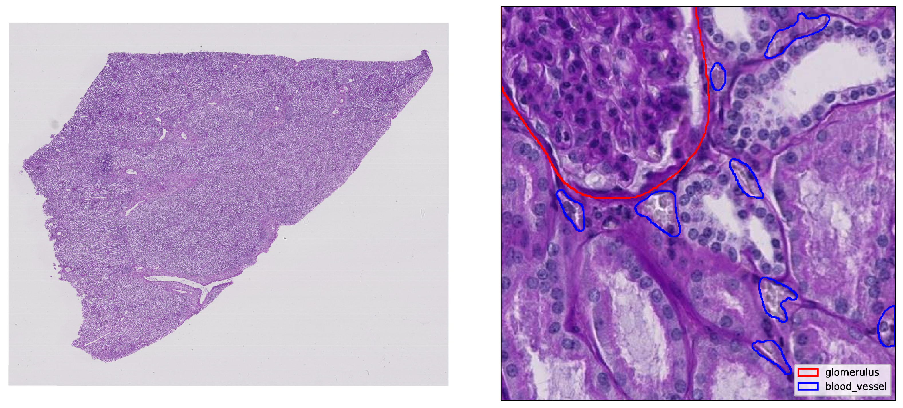
Figure 3.
YOLOv11s-seg training metrics: Mask F1 score (left) and Mask Precision Recall (right).
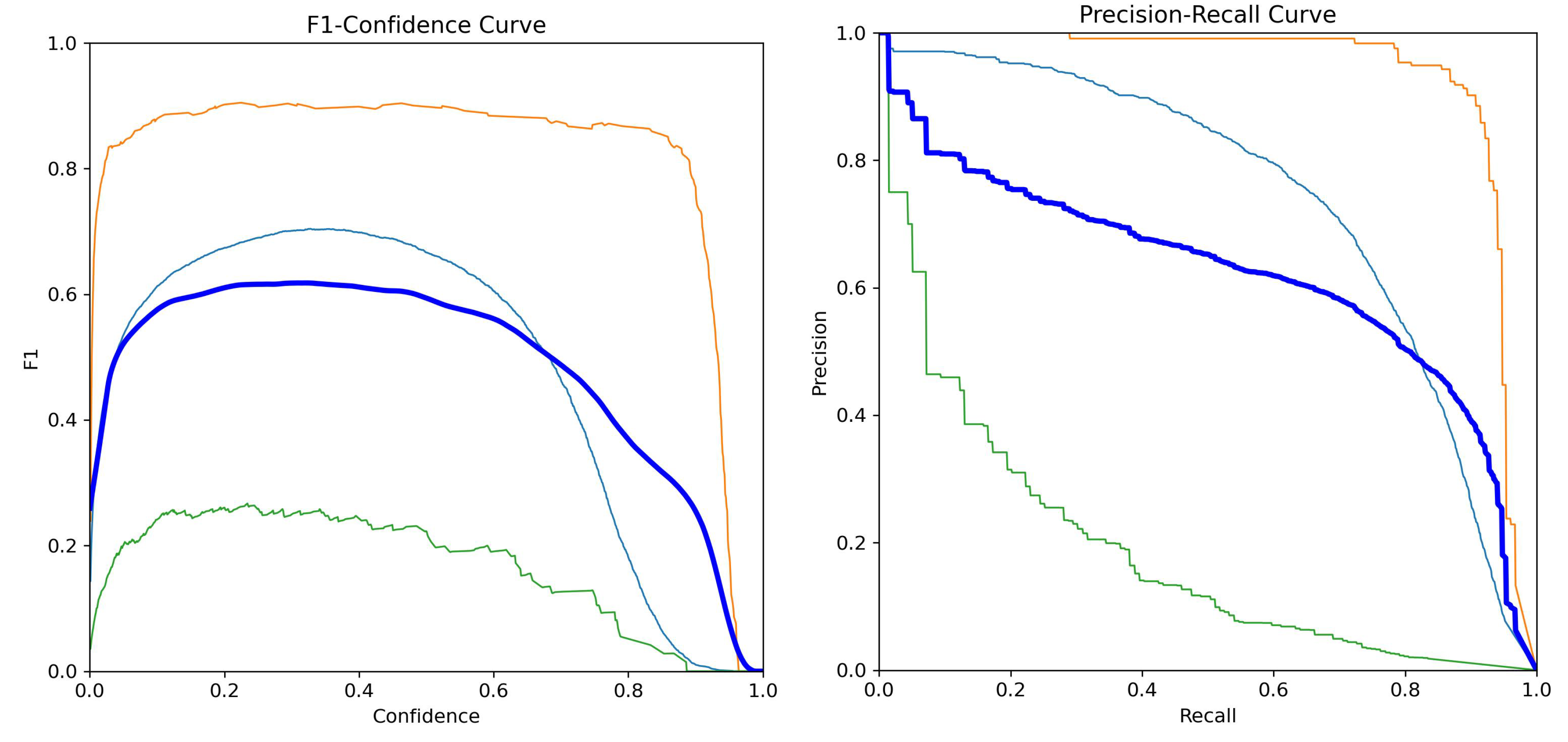
Figure 4.
Validation example: Ground truth (left) and YOLOv11s-seg predicted masks (right) on the same histology tile.
Figure 4.
Validation example: Ground truth (left) and YOLOv11s-seg predicted masks (right) on the same histology tile.
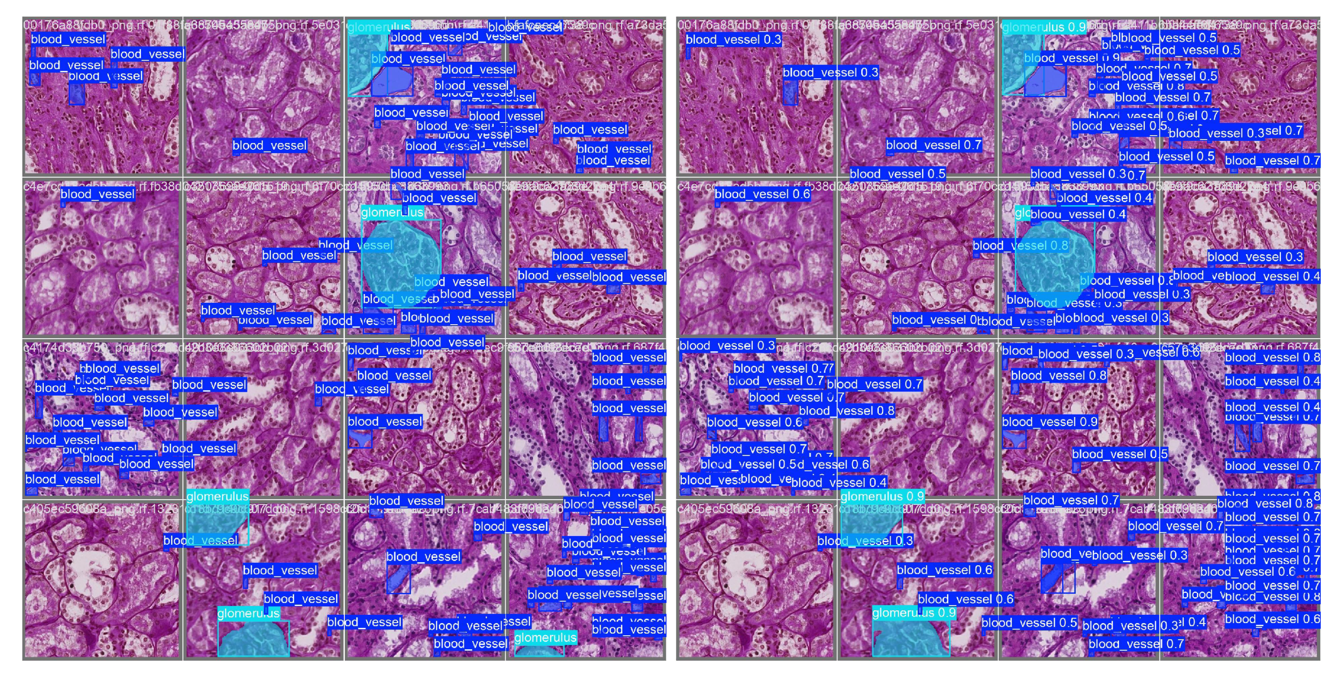
Figure 5.
Performance and computational cost: vs. overlap (left) and inference time per image vs. overlap (right).
Figure 5.
Performance and computational cost: vs. overlap (left) and inference time per image vs. overlap (right).
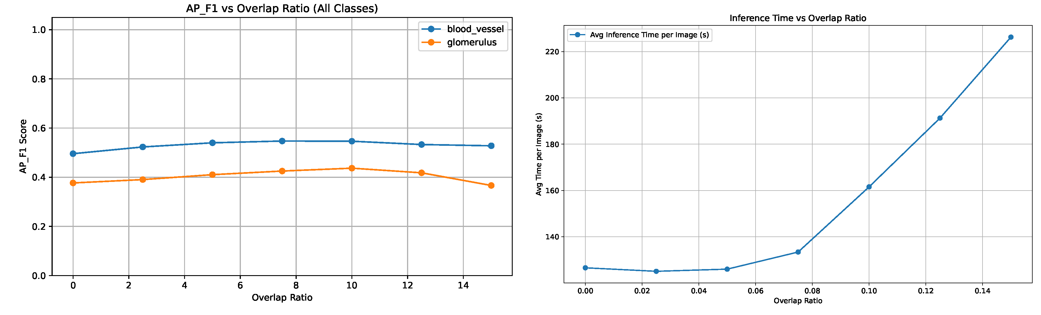
Figure 6.
F1 score across IoU thresholds as a function of overlap ratio for glomeruli (left) and blood vessels (right).
Figure 6.
F1 score across IoU thresholds as a function of overlap ratio for glomeruli (left) and blood vessels (right).
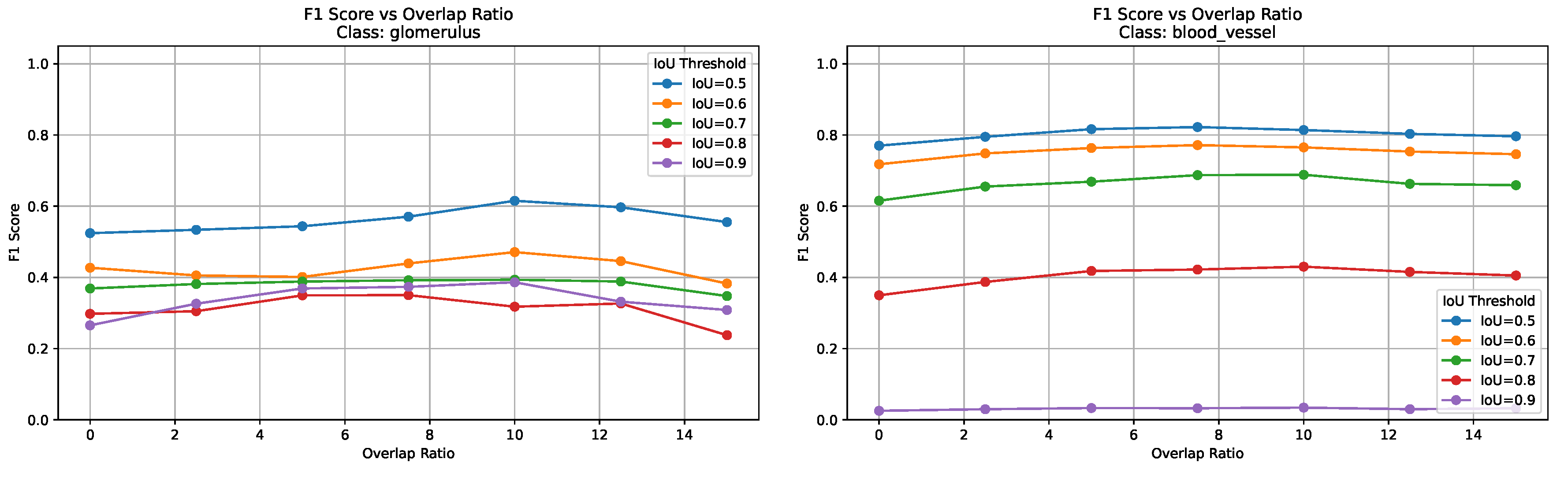
Figure 7.
Performance metrics (accuracy, precision, recall, F1) at IoU = 0.5 across overlap ratios for glomeruli (left) and blood vessels (right).
Figure 7.
Performance metrics (accuracy, precision, recall, F1) at IoU = 0.5 across overlap ratios for glomeruli (left) and blood vessels (right).
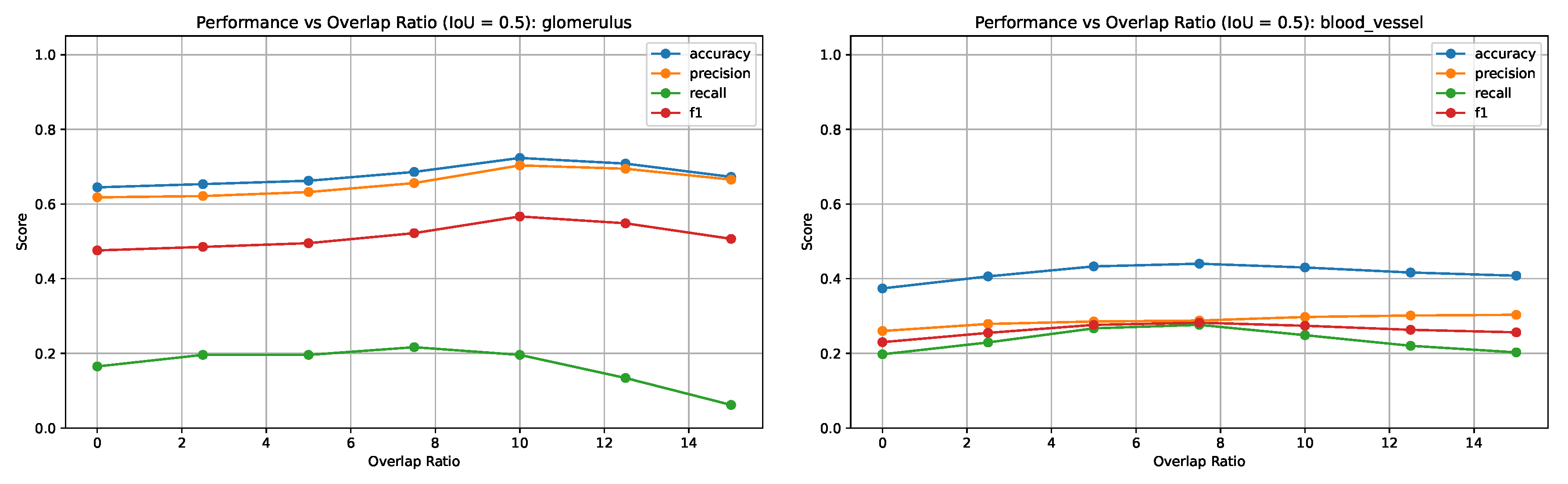
Figure 8.
Instance segmentation results with no overlap (left) and overlap (right).
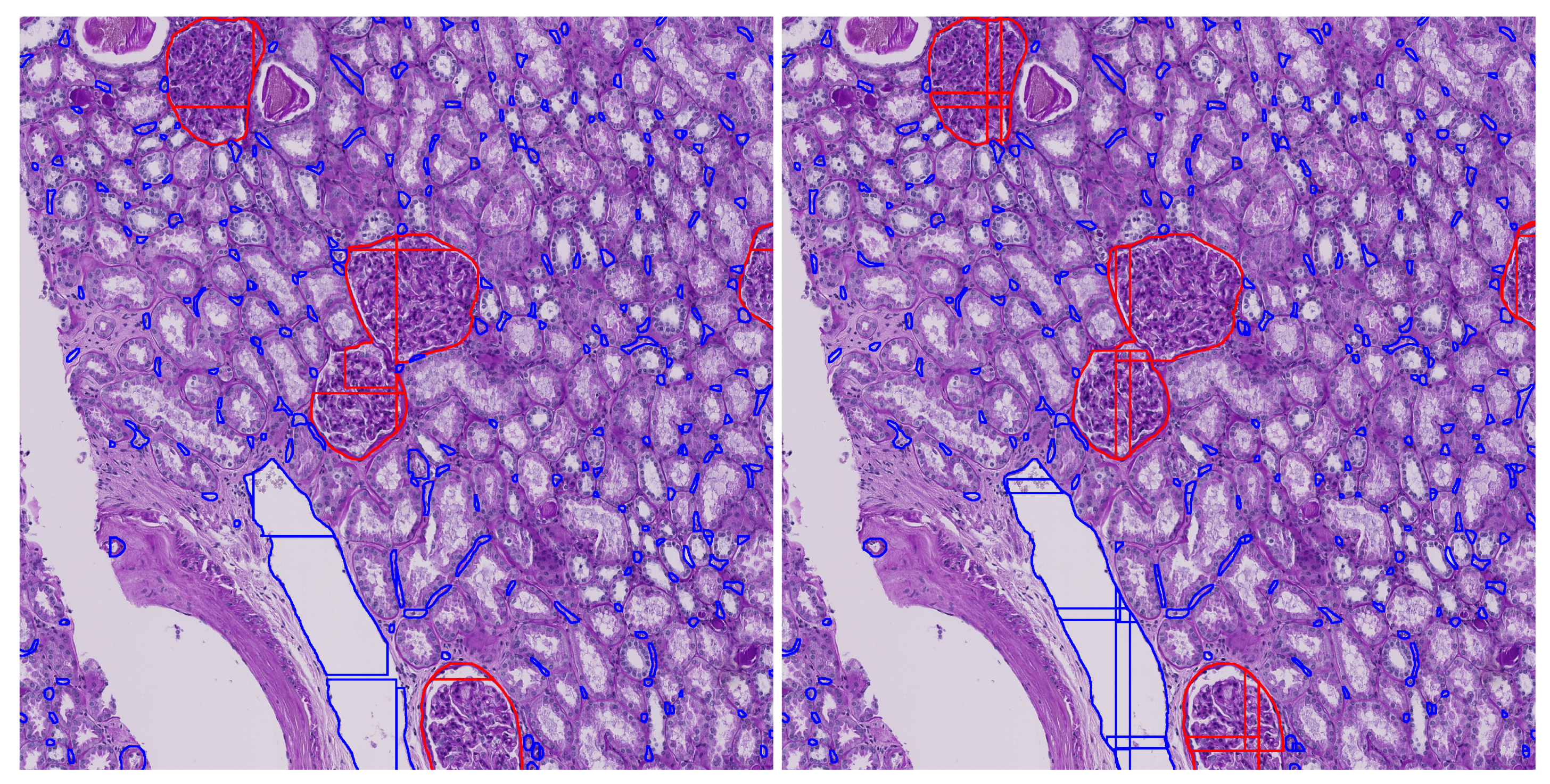
Figure 9.
Convergence and sensitivity analysis.
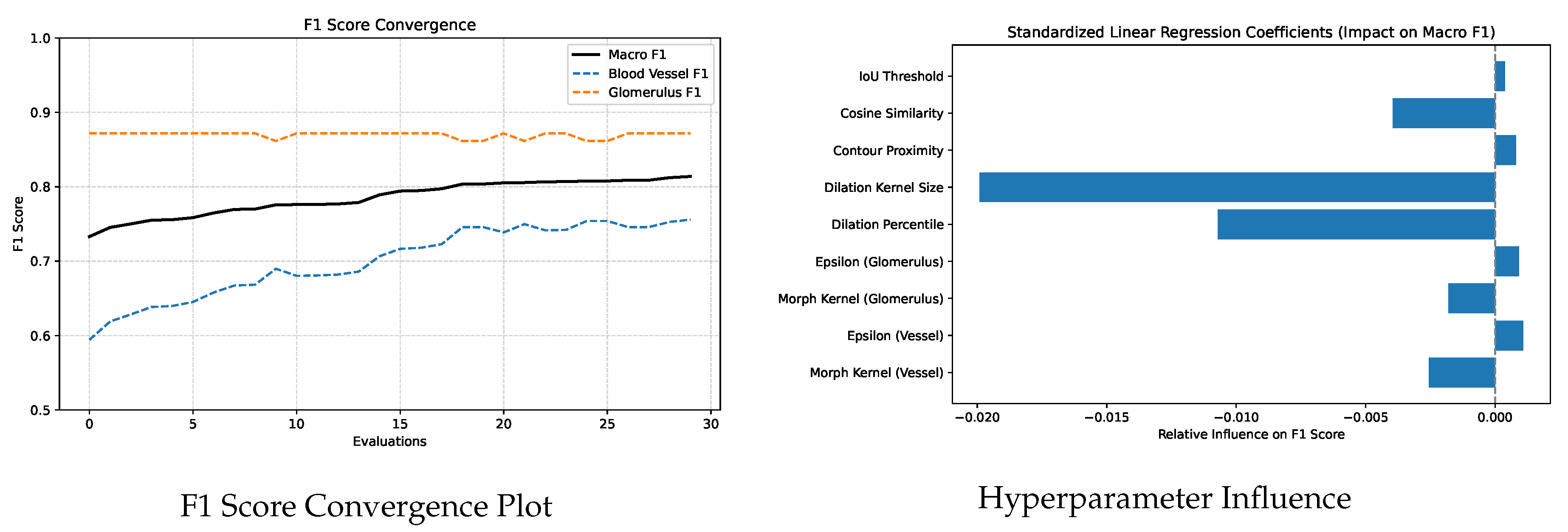
Figure 10.
Qualitative comparison of predicted and ground truth annotations for the best performing image in each class.
Figure 10.
Qualitative comparison of predicted and ground truth annotations for the best performing image in each class.
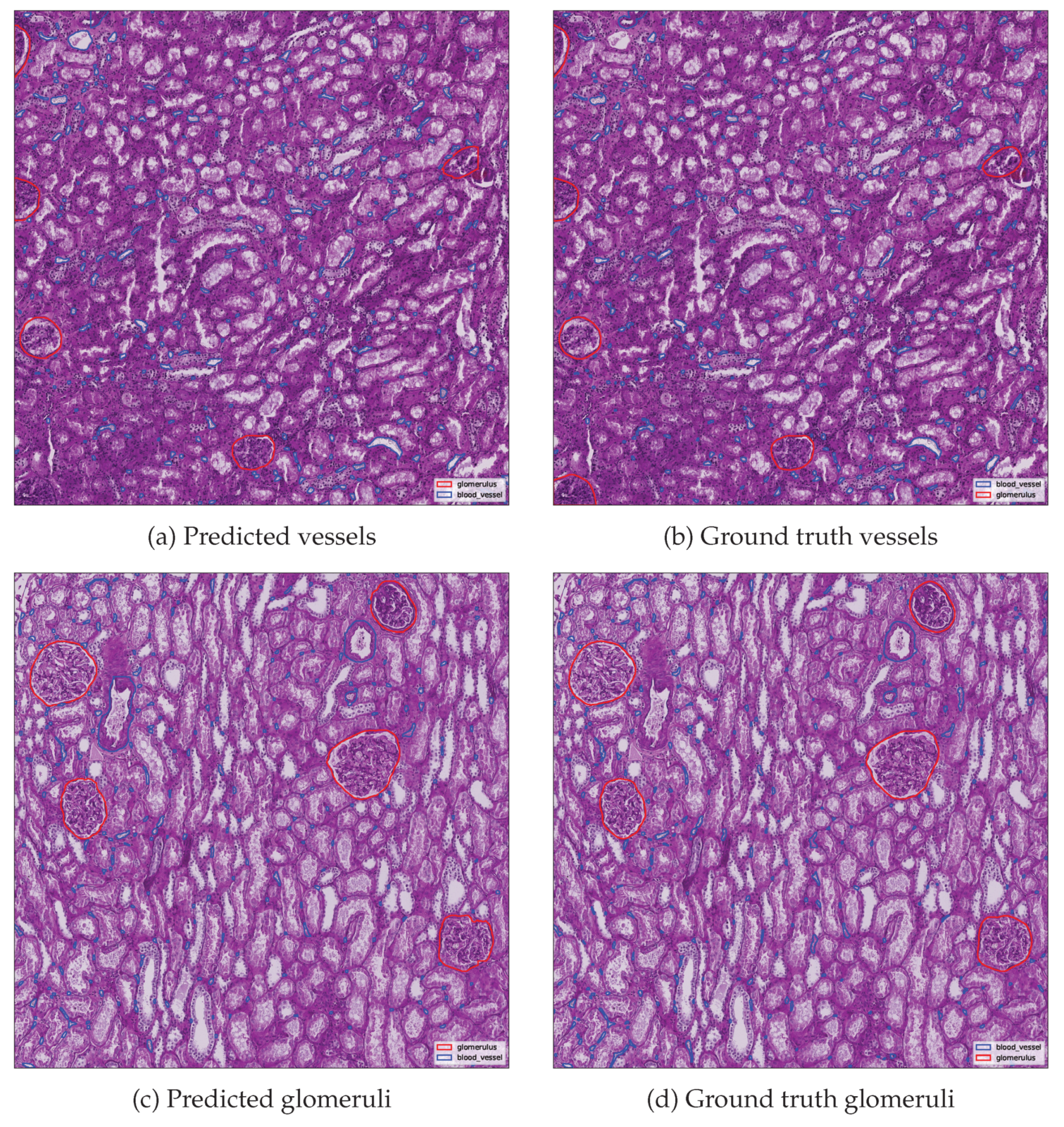
| (a) Predicted vessels | (b) Ground truth vessels |
| (c) Predicted glomeruli | (d) Ground truth glomeruli |

Table 1.
Empirically selected hyperparameter ranges for PSO optimization.
| Hyperparameter | Overall (Range) | Blood Vessels | Glomeruli |
|---|---|---|---|
| morph_kernel | – | 5 to 11 | 3 to 7 |
| epsilon | – | 1.0 to 2.0 | 0.5 to 1.5 |
| dilation_percentile | 5 to 30 | Shared | Shared |
| dilation_kernel | 3 to 11 | Shared | Shared |
| contour_proximity_thresh | 20.0 to 80.0 | Shared | Shared |
| cosine_sim_thresh | 0.80 to 0.95 | Shared | Shared |
| bbox_iou_thresh | 0.05 to 0.50 | Shared | Shared |
Table 2.
Instance segmentation performance comparison of YOLOv11s-seg and YOLOv12s-seg.
| Segment | Instance | Precision (%) | Recall (%) | F1 Score |
|---|---|---|---|---|
| Blood Vessels | YOLOv11s-seg | 73.5 | 67.2 | 0.702 |
| YOLOv12s-seg | 65.6 | 69.8 | 0.676 | |
| Glomeruli | YOLOv11s-seg | 90.5 | 90.8 | 0.906 |
| YOLOv12s-seg | 91.5 | 88.6 | 0.900 | |
| Overall | YOLOv11s-seg | 82.0 | 79.0 | 0.804 |
| YOLOv12s-seg | 77.6 | 76.9 | 0.789 |
Table 3.
Computational efficiency metrics of YOLOv11s-seg and YOLOv12s-seg.
| Metric | YOLOv11s-seg | YOLOv12s-seg | Unit |
|---|---|---|---|
| Time per Epoch | 2:17 | 4:38 | min:s |
| Average Inference Time per Tile | 6.2 | 11.7 | ms |
| GPU Memory Utilization | 5.5 | 8.1 | GB |
| Total Training Time (100 epochs) | 4:02:00 | 6:58:19 | h:m:s |
Table 4.
Best PSO optimized parameters with 7.5% overlap.
| Hyperparameter | F1 Score | Blood Vessels | Glomeruli |
|---|---|---|---|
| morph_kernel (vessel) | 7 | 7 | 7 |
| epsilon (vessel) | 1.07 | 1.10 | 1.50 |
| morph_kernel (glomerulus) | 5 | 5 | 7 |
| epsilon (glomerulus) | 1.31 | 1.47 | 0.95 |
| dilation_percentile | 23 | 5 | 20 |
| dilation_kernel | 5 | 5 | 5 |
| contour_proximity_thresh | 45.97 | 56.24 | 55.46 |
| cosine_sim_thresh | 0.94 | 0.91 | 0.82 |
| bbox_iou_thresh | 0.21 | 0.12 | 0.17 |
| F1 Score | 0.8138 | 0.7559 | 0.8718 |
Table 5.
Evaluation metrics for the best performing annotated examples.
| Metric | Blood Vessel | Glomerulus | ||
|---|---|---|---|---|
| GT | Pred | GT | Pred | |
| Instance Count | 363 | 340 | 5 | 5 |
| True Positives (TP) | 299 | 5 | ||
| False Positives (FP) | 41 | 0 | ||
| False Negatives (FN) | 64 | 0 | ||
| Accuracy | 0.740 | 1.000 | ||
| Precision | 0.879 | 1.000 | ||
| Recall | 0.824 | 1.000 | ||
| F1 Score | 0.851 | 1.000 | ||
Table 6.
Average and maximum improvements () in segmentation metrics after applying the optimized mask merging strategy.
Table 6.
Average and maximum improvements () in segmentation metrics after applying the optimized mask merging strategy.
| Class | Type | Accuracy | Precision | Recall | |
|---|---|---|---|---|---|
| Blood Vessel | Average | 0.0437 | 0.0815 | -0.0058 | 0.0360 |
| Max | 0.1051 | 0.1710 | 0.0201 | 0.0872 | |
| Glomerulus | Average | 0.4234 | 0.4831 | 0.0822 | 0.3571 |
| Max | 0.6944 | 0.6720 | 0.5000 | 0.6652 |
Disclaimer/Publisher’s Note: The statements, opinions and data contained in all publications are solely those of the individual author(s) and contributor(s) and not of MDPI and/or the editor(s). MDPI and/or the editor(s) disclaim responsibility for any injury to people or property resulting from any ideas, methods, instructions or products referred to in the content. |
© 2025 by the authors. Licensee MDPI, Basel, Switzerland. This article is an open access article distributed under the terms and conditions of the Creative Commons Attribution (CC BY) license (http://creativecommons.org/licenses/by/4.0/).
Copyright: This open access article is published under a Creative Commons CC BY 4.0 license, which permit the free download, distribution, and reuse, provided that the author and preprint are cited in any reuse.


