Submitted:
08 July 2025
Posted:
09 July 2025
You are already at the latest version
Abstract
Metaheuristic algorithms are widely used for solving complex optimization problems without relying on gradient information. They efficiently explore large, non-convex, and high-dimensional search spaces but face challenges with dynamic environments, multi-objective goals, and complex constraints. This paper introduces a novel hybrid algorithm, Fick’s Law Algorithm with Opposition-Based Learning (FLA-OBL), combining FLA’s strong exploration-exploitation balance with OBL’s enhanced solution search. Tested on CEC 2017 benchmark functions, FLA-OBL outperformed state-of-the-art algorithms, including the original FLA, in convergence speed and solution accuracy. To address real-world multi-objective problems, we developed FFLA-OBL (Fuzzy FLA-OBL) by integrating a Fuzzy Logic System for UAV path planning with obstacle avoidance. This variant effectively balances exploration and exploitation in complex, dynamic environments, providing efficient, feasible solutions in real time. Experimental results confirm FFLA-OBL’s superiority over the original FLA in both solution optimality and computational efficiency, demonstrating its practical applicability for multi-objective optimization in UAV navigation and related fields.
Keywords:
Fick’s Law Algorithm
; Opposition-Based Learning
; Metaheuristic algorithms
; multi-objective optimization problems
; Fuzzy Logic
; UAV path planning
1. Introduction
As real-world problems continue to grow in complexity and sophistication, there has been a marked increase in the demand for more efficient optimization methods, particularly metaheuristic algorithms, over the past few decades. These problems, in general, are characterized by numerous non-linear constraints, computationally intensive processes, expansive search spaces, and non-convex complexities, all of which pose significant challenges to conventional optimization approaches. As such, solving these intricate problems requires advanced strategies capable of navigating high-dimensional, irregular, and often ill-defined solution landscapes.
Metaheuristic algorithms have, indeed, garnered significant attention and widespread acceptance due to several advantages: (i) flexibility and simplicity in design; (ii) ease of implementation, owing to their intuitive concepts; (iii) the ability to avoid suboptimal regions within the solution space; and (iv) the fact that they do not require knowledge of the objective function gradient. However, it is important to note that metaheuristic algorithms typically aim to find a near-optimal solution, rather than the exact optimal one.
Their operation lies mostly on balancing between two critical search strategies: (1) exploitation/diversification and (2) exploration/intensification. Exploration focuses on globally searching the solution space, which helps in avoiding local optima and mitigating the risk of entrapment in suboptimal regions. In contrast, exploitation involves refining and improving the quality of neighboring promising solutions through localized search. Achieving optimal algorithm performance requires a careful balance between these two complementary strategies. While each algorithm employs these strategies, the specific operators and mechanisms used to implement them vary across different metaheuristics [1,2,3,4].
Another critical aspect that influences the performance of optimization algorithms is population initialization, which significantly impacts the convergence rate. A widely used strategy involves the random generation of the initial population. However, this approach may result in an initial population that is either far from or close to the true optimal solution. In real-time applications, such as navigation or path planning, it is essential to obtain a fast solution while ensuring that the solution remains adequately optimal. As such, the choice of initialization technique becomes crucial, as it directly affects the algorithm's ability to quickly converge to a near-optimal solution while preserving computational efficiency.
The random initialization of solutions can lead to fast convergence, provided the initial guess is relatively close to the optimal solution. However, if the initial guess is significantly distant from the optimal solution, such as being in the worst-case scenario where it is in the opposite direction, the optimization process may take considerably longer or, in extreme cases, become intractable. Naturally, in the absence of any prior knowledge about the problem, it is impossible to make the perfect initial guess. A more rational approach would be to simultaneously explore in all directions, or more specifically, to include the possibility of searching in the opposite direction. For instance, if the goal is to find a solution for , and we hypothesize that searching in the opposite direction might be beneficial, then the first logical step would be to calculate the opposite solution as part of the search process. This strategy helps in efficiently covering the search space, potentially accelerating convergence by leveraging both the direct and opposite search directions. This concept is rooted in Opposition – Based Learning (OBL) , a strategy that aims to enhance the efficiency of optimization algorithms by considering not only the current solution but also its opposite counterpart [5,6].
In recent research, significant efforts have been made to enhance the performance of optimization algorithms by incorporating the concept of Opposition-Based Learning (OBL). For instance, Generalized Opposition-Based Learning (GOBL) combined with Cauchy mutation was utilized in [7] to augment the Particle Swarm Optimization (PSO) algorithm's ability to escape local optima. Similarly, the Firefly Algorithm (FA) was hybridized with OBL to form Opposition-based Firefly Algorithm (OFA), which improved both the convergence speed and exploration capabilities of the algorithm [8]. The Brainstorm Optimization Algorithm (BSO) leveraged chaotic maps and opposition-based learning for initializing solutions and updating the population to enhance its optimization performance [9]. Chaotic Opposition Learning (COL) was also employed to enhance the Grey Wolf Optimization (GWO) algorithm, particularly in continuous global numerical optimization, by mitigating solution stagnation and improving the precision of the search [10]. In [11], an Improved Self-Regulatory Woodpecker Mating Algorithm was introduced, featuring a novel Distance Opposition-Based Learning (DOBL) mechanism aimed at improving exploration, diversity, and convergence in solving optimization problems. Additionally, a dynamic opposition-based learning concept was proposed in [12], in combination with Levy flight, to enhance the prairie dog optimization algorithm's efficiency in addressing global optimization and engineering design challenges.
The concept of OBL is commonly integrated into optimization algorithms, particularly during the stages of population initialization and/or population update, to enhance their performance. Building on the advantages of OBL to boost the efficiency of optimization processes, this study introduces a hybrid optimization algorithm, based on the newly proposed Fick's Law Algorithm (FLA) [13] combined with OBL (FLA-OBL), aimed at improving convergence speed and facilitating local optima avoidance in solving real-world global optimization problems. FLA was selected due to its superior convergence rate and its effective balance between exploration and exploitation. To evaluate the performance of FLA-OBL, the CEC 2017 benchmark suite (IEEE Congress on Evolutionary Computation 2017) [21] is employed for a comprehensive comparison with state-of-the-art optimization algorithms.
To further address complex multi-objective scenarios, such as Unmanned Aerial Vehicle (UAV) path planning with obstacle avoidance, we extend FLA-OBL by integrating a Mamdani-type fuzzy logic inference system (FFLA-OBL). This fuzzy enhancement allows the algorithm to handle conflicting objectives dynamically during solution evaluation. We validate the proposed FFLA-OBL algorithm in simulated UAV path planning tasks and benchmark its performance against baseline FLA, highlighting improvements in path efficiency, safety, and multi-objective trade-offs. UAV path planning is a critical research area, particularly relevant for delivery applications, where efficiency, safety, and adaptability are paramount. With the growing demand for autonomous delivery systems in urban and rural environments, optimizing UAV flight paths ensures timely, energy-efficient, and collision-free deliveries. Real-world delivery scenarios often involve static and dynamic obstacles, no-fly zones, and multiple delivery points, making them ideal testbeds for evaluating the robustness and adaptability of advanced optimization algorithms. By focusing on UAV path planning, especially in delivery contexts, we can address pressing logistical challenges while demonstrating the practical value of the developed algorithms in high-impact, real-time applications with tangible societal and economic benefits.
This work contributes a novel metaheuristic framework based on FLA that leverages opposition learning and fuzzy logic to achieve faster convergence, enhanced solution quality, and greater adaptability in both synthetic benchmarks and real-world optimization applications.
2. Materials and Methods
2.1. Fick’s Law Algorithm (FLA)
The Fick’s Law Algorithm (FLA) is a recently developed physics-inspired optimization method that emulates the principles of Fick’s law to identify stable molecular positions. The FLA operates through three distinct phases corresponding to different modes of particle motion: the diffusion phase, the equilibrium phase, and the steady-state phase. During the diffusion phase, which corresponds to the exploration stage, particles migrate from regions of higher concentration to regions of lower concentration, driven by concentration gradients, in accordance with Fick’s law of diffusion. This phase facilitates broad search across the solution space. Subsequently, the equilibrium phase serves as a transitional stage between exploration and exploitation, wherein concentration gradients equilibrate, and particles relocate based on the identification of the most stable positions within the local region. Finally, the steady-state phase emphasizes exploitation by refining particle positions to achieve an optimal balance between exploration and exploitation. This phase mitigates the risk of premature convergence to local optima by continuously updating particle positions, thereby enhancing convergence stability and solution quality.
The Fick’s Law Algorithm (FLA) (Figure 1) begins with a random initialization, followed by the division of the population into two equal subgroups (subgroups and ). The three phases alternate based on the parameter
where represents the iteration, the maximum number of iterations and is an initial pre-defined parameter (equals with 0.5 in [13]), as follows:
Diffusion Operator
In the diffusion phase the direction of flow () is calculated by:
with and random number in [13]
The number of molecules that will travel to region is determined by:
with in [13] and is the number of molecules of group .
The individual position is updated by:
where is the equilibrium position in region , is the direction factor which equals either that changes randomly and will give high scanning opportunity the given search area and escaping from local optimum, and random number .
is diffusion flux given by:
where in [13] refers to the effective diffusivity constant, and being the mean of molecule position in regions and , respectively, and, eps being the smallest positive number that can be distinguished from zero in a given system.
The other molecules in region are updated by:
where is the equilibrium position in region , and are the upper and lower boundaries of the problem, respectively, and random number .
The molecules in region are updated by:
where random number .
Equilibrium Operator
The Diffusion Rate Factor of each group region is calculated by:
where is the equilibrium location in group and or is the position of particle in group , respectively.
The Group Relative Quantity of the region in group is calculated by:
where , The individual position is updated by:
where is the position of particle in group , or is the equilibrium location in
group or , and the motion step
with and being the best fitness score and the fitness score of particle in group at time , respectively.
Steady State Operator
The Diffusion rate factor is calculated based on:
where is the steady state location, the position of particle of region at time,
The motion step factor is calculated based on:
where and are the best fitness score and the fitness score of particle in group at time , respectively.
The individual position is updated by:
where is the relative quantity of the region .
2.2. Opposition-Based Learning (OBL)
Opposition-Based Learning (OBL) is a relatively novel concept introduced in 2005 [5] and since then numerous artificial and computing intelligence algorithms have been enhanced by utilizing this concept, such as Reinforcement Learning, Neural Networks, numerical optimization algorithms / metaheuristics and Fuzzy Systems, among others. The basic idea of OBL theory is based on the interplay between estimates and counter-estimates, positive and negative weights, and actions versus counter-actions [6]. In the context of Opposition-Based Learning (OBL), the core aim of the optimization algorithm is to determine the optimal solution for an objective function by evaluating both an estimate and its opposite at the same time. This approach can improve the algorithm's performance, since the simultaneous consideration of opposing solutions helps to expand the search space, which may lead to faster convergence and a reduced risk of getting trapped in local optima.
Initially, the definitions of the opposite number, the opposite point and of the opposition-based optimization should be introduced [5,14].
Definition 1. Opposite Number
Let be a real number, where . The opposite number of is defined by
Similarly, the opposite point in higher dimensions is defined.
Definition 2. Opposite Point
Let be a point in n-dimensional space, where . The opposite point of is defined by
Definition 3. Opposition-Based Optimization (OBO)
Let be a point in n-dimensional space used as a candidate solution, and be the fitness function. If , then the point can be replaced by in the set of candidate solutions , otherwise the point remains in . Therefore, both the point and its opposite point are simultaneously evaluated to keep the optimal one.
Population-based algorithms, generally, initiate the optimization process with an initial population, which is often generated randomly. The aim is to iteratively improve this population, ultimately converging to an optimal solution. The process is terminated when the predefined termination criteria are satisfied. Commonly adopted termination criteria include the number of iterations or the number of fitness function’s evaluations. The random initialization of the population, along with the distance of the individuals from an optimal solution affect the computation time and the convergence speed, among others. Based on the probability theory, which suggests that 50% of cases a guess is farther from the solution than its opposite [14], the generation of the initial population can be enhanced by incorporating the opposite candidate solutions, as well. Hence, the initial population is formed either by the initial solutions or its opposites, depending on their evaluation score (Definition 3). This allows a better initial population closer to optimal solution leading to higher convergence speed. Similarly, the OBO approach can be employed not only during the initialization of the population but also integrated into iterative phase of the algorithm to enhance the update process of the population.
2.3. Fick’s Law Algorithm Enhanced with Opposition-Based Learning (FLA-OBL)
Opposition-Based Learning is employed to enhance the operation of FLA algorithm. Specifically, OBL will be used in the initialization of the population and in the update processes of the population (Figure 2).
Population initialization of FLA with OBL
Let assume randomly generated particles following the process of original FLA. In FLA-OBL the initial population will consist of the particles with their opposite points. The rest of the process including the evaluation of the population will remain the same.
Population update of FLA with OBL
After every stage of FLA (diffusion operator, equilibrium operator, and steady-state operator) where the population has been updated the opposite operator will take place. In this stage the opposite population will be generated based on the corresponding opposite points of the particles that form the current population. Every particle with its opposite particle will be evaluated based on the fitness score and the best will be chosen to form the final population.
2.4. Fick’s Law Algorithm Enhanced with Fuzzy Logic and Opposition-Based Learning (FFLA-OBL)
To address real world multi-objective optimization problems the proposed FLA-OBL algorithm will be enhanced with Fuzzy Logic (FFLA-OBL). Specifically, the Mamdani Fuzzy Inference System (FIS) will be integrated into the evaluation process of the FLA-OBL algorithm (Figure 3). In section 3 the implementation of the FIS for the multi-objective path planning problem in case in UAV missions and obstacle avoidance is presented analytically.
3. Mathematical Modeling of UAV Multi-Objective Path Planning Problem
To solve the UAV multi-objective path planning problem the proposed FLA-OBL algorithm will be enhanced with Fuzzy Logic in the evaluation process of the algorithm. The Mamdani FIS will be used for this purpose.
3.1. Mathematical Formulation of the Problem
The UAV multi-objective path planning problem consists of finding the optimal path from an initial position to a desired destination by minimizing the traveled distance (traveled distance objective term), minimizing brute changes during flight (path curvature objective term) and minimizing the penalties/risk for obstacle collision, which means to keep safe distance while passing from obstacles (collision risk objective term). Below, the mathematical modeling of the objective terms are shown:
Traveled distance
Given the set of the discretization points of the path with edges , we calculate with the Euclidean distance the length of the generated path that the UAV has to travel as:
Path curvature
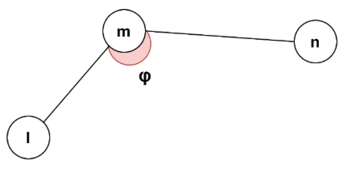
Given the angle that the discretization points and of the path form, we define the path deviations as:
Figure 4.
The formation of the angle from 3 consecutive discretization points and .
Collision risk
The safety term (33) is defined as the sum of mean violation measure (32) computed from the Euclidean distance (31) of each obstacle and the given points which are derived from path’s discretization:
where is the minimum safety distance from obstacles defined by the user (0.3 for the UAV case study in Section 4.3.2) and the radius of the obstacle presented as circle.
3.2. Mamdani Fuzzy Inference System for the Fuzzy FLA-OBL (FFLA-OBL)
The Fuzzy Inference System (FIS) is implemented with the Mamdani inference methodology [15]. Mamdani fuzzy inference system is commonly adopted to multi-objective path planning problems [16,17,18,19,20]. Its advantages can be summarized as: (i) expressive power; (ii) easy formalization and interpretability; (iii) reasonable results with relatively simple structure; (iv) suitable and widely used for decision support applications due to the intuitive and interpretable nature of the rule base; (v) can be used for Multiple Input Single Output and Multiple Input Multiple Output systems; and (vi) the output value can be either crisp or fuzzy [21,22,23]. Given each crisp value, the uncertainty can be modeled by fuzzy sets, where corresponds to the traveled distance term, to the path curvature, to collision risk and to path quality:
representing overlapping value intervals that can be expressed linguistically similarly to the proposed FIS. For this, three fuzzy universes are defined: and representing the universe of discourse for the traveled distance, path’s curvature/smoothness and collision risk, respectively. The universe corresponds to the overall path’s quality. The membership functions are selected based on the possible values of each variable and are illustrated in Figure 5, Figure 6, Figure 7 and Figure 8. In Table 1 the fuzzy rules used in FIS are presented, while Figure 9 illustrates the flowchart of the fuzzy evaluation process integrated in FLA algorithm.
4. Experimental Verification
To examine the effectiveness of the proposed algorithm FLA-OBL a comprehensive evaluation was conducted, which includes: (i) comparison with various state-of-the-art optimization algorithms in CEC2017 testbed; (ii) convergence and fitness landscape analyses; and (iii) comparison of FFLA-OBL with original FLA across multiple scenarios in multi-objective UAV path planning and obstacle avoidance.
The experimental evaluation was implemented in Python 3.10 using a Windows 11 Pro 64-bit operating system with a 3.9 GHz CPU and 32 GB RAM.
4.1. Testbed for Computational Analysis of FLA-OBL
The FLA-OBL algorithm was evaluated against a range of state-of-the-art optimization algorithms (2016-2023), spanning various categories, including nature-inspired metaheuristics, physics-inspired metaheuristics, swarm intelligence-based metaheuristics, evolutionary metaheuristics, and hybrid approaches (Table 2). Specifically, Hunger games search (HGS) [24] is a population-based metaheuristic that mimics the logic of the collaborative interactions based on individual hunger. Chaotic Local Search-Based Differential Evolution Algorithm (CJADE) [25] incorporating chaotic local search (CLS) mechanisms into the well-known differential evolution (DE) algorithm JADE. Hybrid Salp Swarm-Harris Hawks optimization algorithm (HSSAHHO) [26] is a modern, hybrid optimization algorithm that combines the strengths of Salp Swarm Algorithm (SSA) and Harris Hawks Optimization (HHO). The Salp Swarm Algorithm (SSA) is a nature-inspired optimization algorithm based on the collective movement of salps (a type of jellyfish). Harris Hawks Optimization (HHO) is an optimization algorithm inspired by the hunting behavior of Harris' hawks. Ensemble Particle Swarm Optimizer (EPSO) [27] is a metaheuristic optimization algorithm that integrates the strengths of multiple Particle Swarm Optimization (PSO) models into an ensemble learning framework to improve the performance and robustness of solving optimization problems. The Whale Optimization Algorithm (WOA) [28] is a nature-inspired metaheuristic optimization algorithm based on the hunting behavior of humpback whales. Emotion-aware Brainstorm Optimization (EBO) [29], is inspired by the attraction-repulsion mechanism of electromagnetism, and it is applied in a new emotion-aware brainstorming context, where positive and negative thoughts produce ideas interacting with each other. Hybrid Teaching Learning Optimization Algorithm (HTLBO) [30] is an evolutionary algirthm that employs a group of learners or a class of learners to perform global optimization search process. The original FLA algirithm is also included.
To assess FLA-OBL’s consistency and reliability, the under-consideration algorithms were constructed with the same number of iterations (1000) and population size (30), respectively, to provide a fair comparison in CEC2017. The CEC 2017 (IEEE Congress on Evolutionary Computation 2017) consists of a set of benchmark functions commonly used to test optimization algorithms. These functions are used to evaluate the performance of algorithms in solving real-world optimization problems [31]. The CEC2017 consists of 2 unimodal functions (F1-F2), 7 simple multimodal functions (F3-F9), 10 hybrid functions (F10-F19), and 10 composition functions (F20-F29) [31]. It is important to highlight that the second function in the CEC2017 suite (F2) was excluded from the evaluation due to its instability, particularly at higher dimensions [32].
The experimental evaluation was conducted following established standard experimental protocols [33]. To assess the performance of the compared algorithms, the results were subjected to rigorous statistical analysis. For each optimization problem, 20 runs were performed for 30 dimensions where the average of the results (mean) and standard deviation (std) have been reported. Additionally, performance comparisons of the algorithms were supplemented by non-parametric, rank-based tests, specifically the Mann-Whitney U (MWU) test and the Friedman test. The MWU test was employed on the results obtained from pairwise comparisons between the FLA-OBL algorithm and the competing algorithms. The MWU is first conducted on the results of the 20 runs for each function among the competed algorithms. Subsequently, the Friedman test is applied among all competed algorithms per function categories (unimodal, multimodal, hybrid and composition functions).
For post-hoc statistical analysis, MWU tests (α = 0.05) with Holm p-value correction [34] were performed, using the results obtained from independent algorithm runs to rank the algorithms’ performance. This methodological framework was selected due to its recognition as a robust approach for comparing swarm and evolutionary algorithms in the literature [35,36,37].
4.2. Convergence and Fitness Landscape Analyses
Most population-based metaheuristic algorithms are designed to balance the capabilities of divergence and convergence. Divergence (or exploration) enables the algorithm to explore the search space for potential new regions, while convergence (or exploitation) focuses on refining solutions within known regions of interest [29,38,39]. Consequently, the convergence capability reflects the efficiency of the selection and evolution processes employed in FLA-OBL. Divergence, on the other hand, is facilitated by the OBL operator, highlighted in previous studies [6,40]. In the following, convergence and fitness landscape analyses are conducted to evaluate the contributions of the proposed strategies in FLA-OBL, in comparison to traditional FLA and the two most competitive algorithms based on their performance on CEC2017.
To assess the effectiveness of the proposed algorithm relative to the original FLA, a convergence velocity analysis and Dynamic Fitness Landscape Analysis (DFLA) were conducted to evaluate the convergence and divergence characteristics of FLA-OBL. For the convergence analysis, the following metrics were utilized: (i) Expected Quality Gain (EQG) and (ii) Expected Change (EC) in the distance to the global optimum. These metrics were selected to provide a comprehensive evaluation of the algorithm's ability to approach optimal solutions and navigate the search space effectively [29,41,42]:
The where and are the global optimum and the best-found solution at iteration , respectively.
The divergence analysis is grounded in Dynamic Fitness Landscape Analysis (DFLA), a widely used framework for assessing the effectiveness of population-based metaheuristic algorithms [29,41,42]. In this context, three key metrics—evolutionary probability, evolutionary ability, and evolvability—were considered to evaluate the algorithm's divergence capabilities. These metrics are quantified using the following measures:
The Evolutionary Probability of a Population (EPP) characterizes the collective behavior of the entire population. Given an initial individual and the generated population , the EPP is defined as the probability that an individual from the population will evolve or transition toward a more optimal solution over successive generations. This metric provides insight into the population's overall capacity for exploration and the likelihood of finding better solutions within the search space:
where is the set of evolved individuals in the population for a minimization problem, and represents the cardinality of the respective sets.
The Evolutionary Ability of a Population (EAP) quantifies the average evolutionary capacity of an initial individual as it progresses through its evolved population. It reflects the population's potential to improve the quality of the individual’s solution over time. This metric helps assess how effectively the population as a whole contributes to the improvement of the initial individual’s solution over generations. The EAP is estimated by the following equation:
where is the standard deviation of the fitness values of the population .
The Evolvability of a Population (EVP) represents the average evolutionary ability across the entire set of the generated population. It captures how effectively the entire population, on average, can evolve toward better solutions over time. This metric provides a holistic view of the population’s overall ability to evolve, integrating both the likelihood of evolution (EPP) and the actual capacity for improvement (EAP) across all individuals. Given the Evolutionary Probability (EPP) and the Evolutionary Ability (EAP), the EVP can be estimated as:
4.3. Evaluation Metrics for the UAV Multi-Objective Path Planning with FFLA-OBL
The evaluation methodology integrates both qualitative and quantitative assessments to provide a comprehensive analysis of algorithmic performance. Qualitative evaluation involves the visual inspection of the generated paths, enabling a comparative analysis of trajectory characteristics across competed algorithms. Quantitative evaluation, similar to [19,20,43,44], is conducted based on the following:
- The objective criteria: (i) traveled distance; (ii) path’s curvature; and (iii) safety, each reflecting critical aspects of path efficiency and feasibility.
- Path quality based on the defuzzification value of Mamdani FIS (Fuzzy evaluation)
- The relative percentage deviation (RPD), quantifying each algorithm's deviation from the best-known solutions:where is the best solution with the highest path quality value; and is the path quality value of the examined solution. Based on the above equations, it is obvious that the lowest values of RPD indicate the preferable solution based on the satisfaction of objective criteria.
5. Results
5.1. CEC 2017 Testbed
Table 3 presents the performance results of the compared algorithms on the CEC2017 benchmark set, along with their corresponding rankings. Specifically, for each benchmark function, the algorithms are ranked from 1 to 9 based on the results from the 20 independent runs and the Wilcoxon rank-sum tests (α = 0.05) with Holm p-value correction. Figure 10 depicts the relative ranking of each algorithm across different categories of benchmark functions. Table 4 shows the results of the Friedman test for all competed algorithms per function categories.
5.2. Convergence Velocity and Fitness Landscape Analyses
The convergence velocity and fitness landscape analyses were conducted to compare the performance of FLA-OBL with baseline FLA and the two most competitive algorithms (EBO and HTLBO) from subsection 5.1 on 7 functions of CEC 2017 benchmark where FLA-OBL presented high and low performance: 1 unimodal, 2 multimodal, 2 hybrid and 2 composition functions. Table 5 presents the average results for both convergence velocity and DFLA of FLA-OBL and competed algorithms (FLA, EBO and HTLBO).
In this subsectin the results from the multi-objective path planning case study are presented. In Table 6 the results of FLA and FFLA-OBL for 3 UAV path planning scenarios with increasing complexity are shown with respect to the evalulation criteria. Error! Reference source not found.-Error! Reference source not found. depict the paths derived from the competed algorithms, FFLA-OBL and FLA, for Scenario 1, 2 and 3 respectively.
Figure 11.
Optimal path and convergence plots generated by (a,c) FLA and (b,d) FFLA-OBL for a scenario with few (7) obstacles.
Figure 11.
Optimal path and convergence plots generated by (a,c) FLA and (b,d) FFLA-OBL for a scenario with few (7) obstacles.
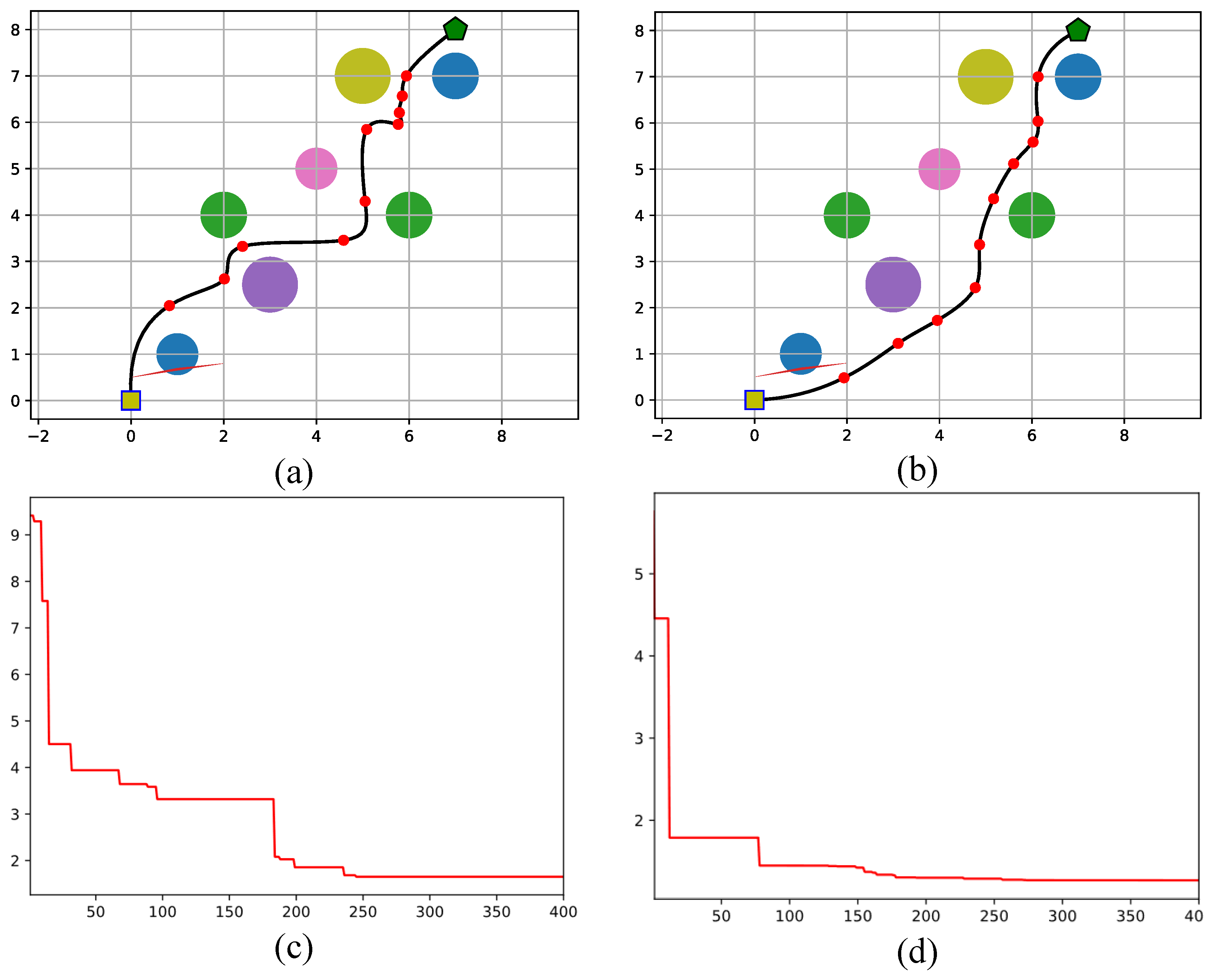
Figure 12.
Optimal path and convergence plots generated by (a,c) FLA and (b,d) FFLA-OBL for a scenario with 12 obstacles.
Figure 12.
Optimal path and convergence plots generated by (a,c) FLA and (b,d) FFLA-OBL for a scenario with 12 obstacles.
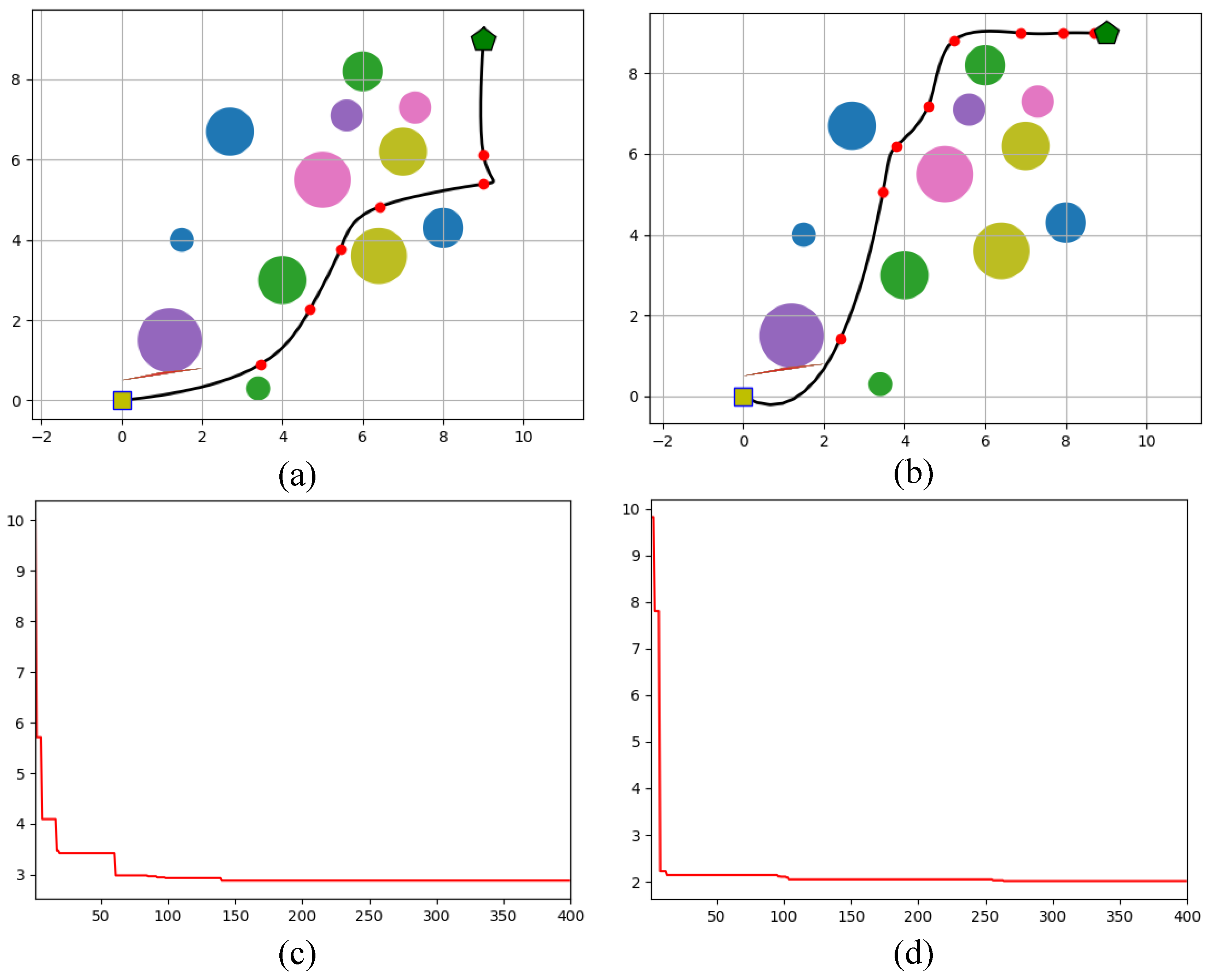
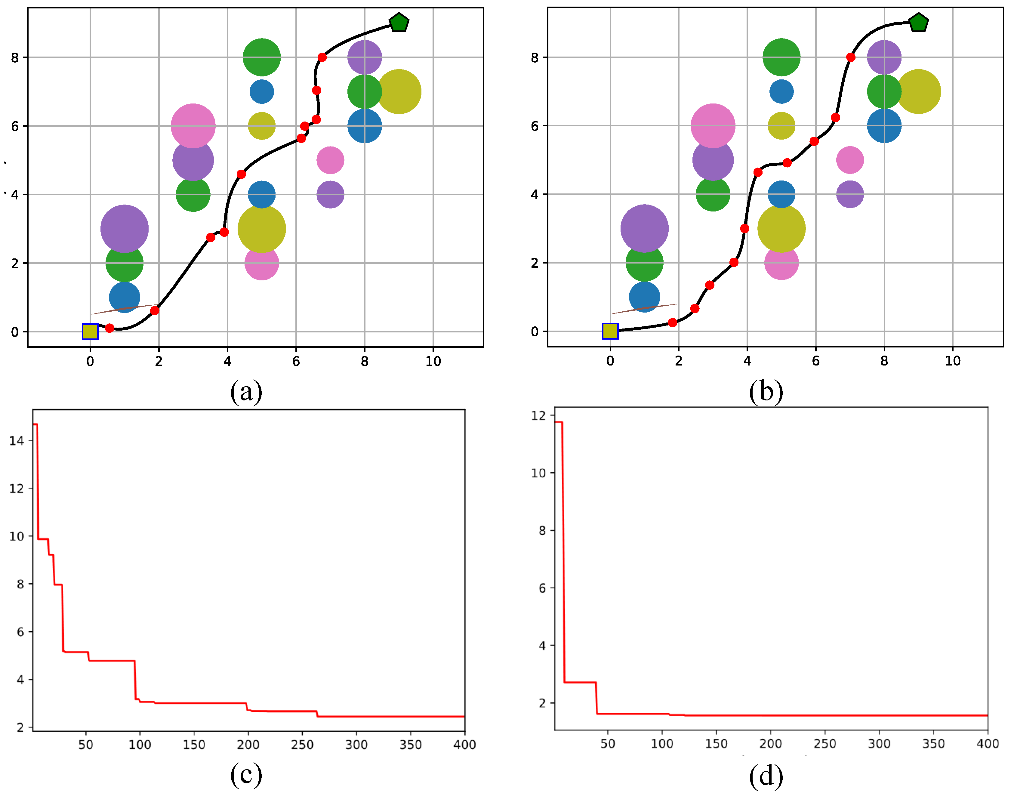
Figure 13.
Optimal path and convergence plots generated by (a,c) FLA and (b,d) FFLA-OBL for a scenario with many (18) obstacles.
Figure 13.
Optimal path and convergence plots generated by (a,c) FLA and (b,d) FFLA-OBL for a scenario with many (18) obstacles.
6. Discussion
The performance analysis across the 28 benchmark functions of CEC2017 reveals notable differences among the tested algorithms in terms of accuracy, stability, and overall effectiveness. The FLA-OBL algorithm consistently achieved the lowest average ranks and demonstrated a strong balance between mean performance and stability, indicating superior accuracy and reliability across diverse problem landscapes. Similarly, EBO also exhibited competitive results, often ranking just behind FLA-OBL, though with slightly higher variability. In contrast, algorithms such as HTLBO and CJADE showed more fluctuating performance; while occasionally achieving top ranks on certain functions, their inconsistency suggests sensitivity to problem characteristics. Algorithms HSSAHHO and EPSO generally underperformed, with higher average mean values and standard deviations, reflecting less precise and less stable outcomes. Overall, the study indicates that FLA-OBL offers a robust and efficient approach suitable for a broad range of optimization problems, while other methods may be more specialized or require further tuning to achieve comparable performance.
The evaluation of algorithm performance across different types of benchmark functions provides deeper insights into their strengths and weaknesses. For the unimodal function F1, which primarily tests exploitation ability, algorithms like FLA-OBL and EBO demonstrated superior performance with lower mean values and stable results, indicating strong convergence capabilities. When considering simple multimodal functions (F3 to F9), which challenge an algorithm’s ability to escape local optima, the performance gap widened. While FLA-OBL and remained the most competitive, algorithms such as HTLBO and CJADE exhibited more variable results, suggesting potential difficulties in balancing exploration and exploitation. Hybrid functions (F10 to F19), combining features of unimodal and multimodal landscapes, further tested algorithm adaptability. Here, the best-performing methods still maintained robust performance, but the increased complexity led to higher standard deviations for most algorithms, reflecting challenges in consistently navigating complex search spaces. However, FLA-OBL remained the most effective algorithm also in this category. Finally, the composition functions (F20 to F29), designed to simulate real-world optimization problems with intricate and diverse landscapes, proved the most challenging. In this category, FLA-OBL showed relative resilience, when most of the competed algorithms presented an increase in mean errors and rank variability highlighted the difficulty of maintaining high performance across multifaceted environments. These observations emphasize that while some algorithms excel in simpler or more structured problems, only a few maintain robust performance across increasingly complex and realistic function types, underlining the effectiveness of FLA-OBL’s adaptive mechanisms and balanced search strategies.
Based on the statistical analysis using MWU tests, FLA-OBL demonstrated significantly superior performance in 178 cases, exhibited statistically equivalent performance in 12 cases, and was significantly outperformed in only 23 cases (Table 3). Furthermore, FLA-OBL achieved statistically significant improvements across all categories of benchmark functions, including unimodal, simple multimodal, hybrid, and composition functions (Table 4). Post-hoc comparisons further confirmed that FLA-OBL consistently outperformed all competing algorithms in each function category, as illustrated in Figure 10.
Further analysis evaluates FLA-OBL with the most competitive algorithms EBO, HTLBO, and baseline FLA, across seven benchmark functions (F1, F5, F7, F16, F19, F21, F26) using three dynamic performance metrics: EQG, EC and EVP (Table 5). FLA-OBL demonstrated the strongest convergence performance, with the highest EQG (0.346) and highest EC (0.430) across all functions. This suggests that FLA-OBL not only converges effectively (high quality gain), but also maintains healthy population movement, avoiding premature stagnation. It balances exploitation and exploration dynamically, enabling it to escape local optima and reach better-quality solutions. EBO and HTLBO follow, with moderate EQG (0.214 and 0.231) and EC (0.249 and 0.272), respectively. HTLBO showed a slightly better convergence profile than EBO in terms of EQG but was slightly slower in EC, suggesting that it improves solution quality with a more stable (less erratic) search pattern. FLA presented the lowest EQG (0.107) and lowest EC (0.115), indicating slow convergence and limited search progression.
In terms of fitness landscape analysis, FLA-OBL again leads with the highest EVP (0.656), indicating that its population maintains high adaptability. This is particularly valuable in complex or rugged landscapes, where adaptability can help discover global optima despite misleading gradients or deceptive valleys. HTLBO and EBO show competitive EVP values (0.493 and 0.447), suggesting that both algorithms retain reasonable diversity and mutation capacity, especially on multimodal or deceptive functions (like F7, F16, and F19). FLA performs weakest in terms of EVP (0.326), confirming its low adaptability in dynamic landscapes. Low EVP implies reduced diversity and a high risk of premature convergence, likely a result of overly greedy or static search dynamics. These findings suggest that FLA-OBL is more effective in navigating complex search spaces and achieving high-quality solutions more efficiently than its counterparts.
In the context of multi-objective UAV path planning for real-world applications such as autonomous delivery, FFLA-OBL demonstrated superior effectiveness compared to the baseline FLA. The enhanced performance of FFLA-OBL indicates its improved capability in handling the trade-offs between multiple conflicting objectives, making it more suitable for complex, real-world UAV mission planning scenarios.
Specifically, in Scenario 1 of path planning with 7 Obstacles, the algorithms were tasked with finding the optimal path while avoiding 7 static obstacles. The FLA algorithm achieved a traveled distance of 13.64 units (Euclidean distance), with a path deviation of 5 brut turns and a collision risk penalty of 0.11. The path quality was rated at 0.75, and the relative performance deviation (RPD%) was 15%. In contrast, FFLA-OBL demonstrated superior performance, with a traveled distance of 10.97 units, significantly shorter than FLA. It had a lower path deviation of 3 and achieved no penalty in terms of collision risk (0), reflecting a highly efficient path planning process. The path quality improved to 0.88.
For the second scenario with 12 Obstacles, which involved a more complex environment with 12 obstacles, FLA resulted in a traveled distance of 15.72 units, a path deviation of 3 brut turns, and a penalty (collision risk) of 0.46. The path quality was measured at 0.62, and the RPD% was 23%, showing a noticeable drop in efficiency when compared to the previous scenario. On the other hand, FFLA-OBL excelled in this scenario as well, with a traveled distance of 11.73 units, a path deviation of 3 brut turns, and a minimal collision risk penalty of 0.08, significantly lower than FLA. The path quality was rated at 0.77, and the RPD% was 0, indicating that FFLA-OBL achieved the optimal solution.
In the most complex scenario, involving 18 obstacles, FLA resulted in a traveled distance of 16.43 units, a path deviation of 8 brut turns, and a penalty (collision risk) of 0.37, reflecting a higher complexity of path planning. The path quality decreased to 0.52, and the RPD% was 27%, which was the highest among the three scenarios, indicating a considerable deviation from the optimal solution. FFLA-OBL, however, performed more efficiently in this challenging scenario, with a traveled distance of 13.89 units, a path deviation of 4 brut turns, and no penalty (collision risk) (0). The path quality was 0.71, and the RPD% was 0, again indicating that FFLA-OBL achieved the optimal solution, even in a highly cluttered environment.
The results across all three scenarios clearly demonstrate the effectiveness of the FFLA-OBL algorithm in comparison to FLA. The FFLA-OBL consistently outperformed FLA in all evaluation criteria, particularly in terms of traveled distance, collision risk, and path quality in obstacle-rich environments. The absence of any collision penalties in FFLA-OBL in all scenarios suggests that the integration of Opposition-Based Learning (OBL) and Fuzzy Logic significantly improves the algorithm's ability to explore the search space and avoid obstacles more efficiently making it suitable for UAV path planning tasks, especially in complex, multi-objective scenarios.
7. Conclusions
This study presents a comprehensive evaluation of the FLA-OBL and FFLA-OBL algorithms across standardized benchmark functions and real-world UAV path planning scenarios. The results from the CEC2017 benchmark suite clearly demonstrate the superior performance of FLA-OBL in terms of accuracy, stability, and adaptability. It consistently achieved the lowest average ranks across various function categories, outperforming state-of-the-art algorithms such as EBO and HTLBO. Statistical validation through the Mann–Whitney U test confirmed the significance of these findings, with FLA-OBL exhibiting superior performance in the vast majority of test cases. Further analysis revealed that its enhanced convergence acceleration, evolvability, and exploration-exploitation balance, attributed to the Opposition-Based Learning (OBL) mechanism, make it robust across both simple and complex optimization problems. Extending these findings to a real-world application, the FFLA-OBL variant demonstrated marked improvements over the baseline FLA in multi-objective UAV path planning. Across multiple increasingly complex scenarios involving obstacle avoidance, FFLA-OBL consistently achieved more optimal paths, lower collision risk, and higher path quality, underscoring its effectiveness in practical, dynamic environments. Overall, the integration of OBL and fuzzy logic significantly enhances the performance and adaptability of the base algorithm, making FLA-OBL and its fuzzy-enhanced variant promising tools for both theoretical optimization challenges and real-world autonomous systems.
Despite the promising results, the current work has several limitations. The evaluation primarily relies on synthetic benchmark functions and a limited set of static UAV path planning scenarios, which may not fully capture the complexity of dynamic real-world environments. Additionally, the study does not explore the computational cost of the proposed algorithms in high-dimensional settings. Future work should address these aspects to further validate and extend the utility of FLA-OBL and FFLA-OBL in diverse and real-time applications.
Author Contributions
Conceptualization, C.N.; methodology, C.N.; software, C.N.; validation, C.N.; formal analysis, C.N.; investigation, C.N.; resources, C.N.; data curation, C.N.; writing—original draft preparation, C.N.; writing—review and editing, C.N.; visualization, C.N.; supervision, C.N.; project administration, C.N.. All authors have read and agreed to the published version of the manuscript.
Funding
This research received no external funding.
Data Availability Statement
Data available on request due to restrictions.
Acknowledgments
We would like to thank the authors of [13] for making available the source codes of FLA used in this study.
Conflicts of Interest
The authors declare no conflicts of interest.
References
- Xu, J.; Zhang, J. Exploration-Exploitation Tradeoffs in Metaheuristics: Survey and Analysis. In Proceedings of the Proceedings of the 33rd Chinese Control Conference; July 2014; pp. 8633–8638.
- Črepinšek, M.; Liu, S.-H.; Mernik, M. Exploration and Exploitation in Evolutionary Algorithms: A Survey. ACM Comput. Surv. 2013, 45, 35:1-35:33. [CrossRef]
- Hussain, K.; Salleh, M.N.M.; Cheng, S.; Shi, Y. On the Exploration and Exploitation in Popular Swarm-Based Metaheuristic Algorithms. Neural Comput & Applic 2019, 31, 7665–7683. [CrossRef]
- Cuevas, E.; Diaz, P.; Camarena, O. Experimental Analysis Between Exploration and Exploitation. In Metaheuristic Computation: A Performance Perspective; Cuevas, E., Diaz, P., Camarena, O., Eds.; Springer International Publishing: Cham, 2021; pp. 249–269 ISBN 978-3-030-58100-8.
- Tizhoosh, H.R. Opposition-Based Learning: A New Scheme for Machine Intelligence. In Proceedings of the International Conference on Computational Intelligence for Modelling, Control and Automation and International Conference on Intelligent Agents, Web Technologies and Internet Commerce (CIMCA-IAWTIC’06); August 2005; Vol. 1, pp. 695–701.
- Mahdavi, S.; Rahnamayan, S.; Deb, K. Opposition Based Learning: A Literature Review. Swarm and Evolutionary Computation 2018, 39, 1–23. [CrossRef]
- Wang, H.; Wu, Z.; Rahnamayan, S.; Liu, Y.; Ventresca, M. Enhancing Particle Swarm Optimization Using Generalized Opposition-Based Learning. Information Sciences 2011, 181, 4699–4714. [CrossRef]
- Abedi, M.; Gharehchopogh, F.S. An Improved Opposition Based Learning Firefly Algorithm with Dragonfly Algorithm for Solving Continuous Optimization Problems. Intelligent Data Analysis 2020, 24, 309–338. [CrossRef]
- Oliva, D.; Elaziz, M.A. An Improved Brainstorm Optimization Using Chaotic Opposite-Based Learning with Disruption Operator for Global Optimization and Feature Selection. Soft Comput 2020, 24, 14051–14072. [CrossRef]
- Adegboye, O.R.; Feda, A.K.; Ojekemi, O.S.; Agyekum, E.B.; Hussien, A.G.; Kamel, S. Chaotic Opposition Learning with Mirror Reflection and Worst Individual Disturbance Grey Wolf Optimizer for Continuous Global Numerical Optimization. Sci Rep 2024, 14, 4660. [CrossRef]
- Karimzadeh Parizi, M.; Keynia, F.; Khatibi bardsiri, A. OWMA: An Improved Self-Regulatory Woodpecker Mating Algorithm Using Opposition-Based Learning and Allocation of Local Memory for Solving Optimization Problems. Journal of Intelligent & Fuzzy Systems 2021, 40, 919–946. [CrossRef]
- Biswas, S.; Shaikh, A.; Ezugwu, A.E.-S.; Greeff, J.; Mirjalili, S.; Bera, U.K.; Abualigah, L. Enhanced Prairie Dog Optimization with Levy Flight and Dynamic Opposition-Based Learning for Global Optimization and Engineering Design Problems. Neural Comput & Applic 2024, 36, 11137–11170. [CrossRef]
- Hashim, F.A.; Mostafa, R.R.; Hussien, A.G.; Mirjalili, S.; Sallam, K.M. Fick’s Law Algorithm: A Physical Law-Based Algorithm for Numerical Optimization. Knowledge-Based Systems 2023, 260, 110146. [CrossRef]
- Rahnamayan, S.; Tizhoosh, H.R.; Salama, M.M. Opposition-Based Differential Evolution (ODE) with Variable Jumping Rate. In Proceedings of the 2007 IEEE Symposium on Foundations of Computational Intelligence; IEEE, 2007; pp. 81–88.
- Harliana, P.; Rahim, R. Comparative Analysis of Membership Function on Mamdani Fuzzy Inference System for Decision Making. J. Phys.: Conf. Ser. 2017, 930, 012029. [CrossRef]
- Ntakolia, C.; Lyridis, D.V. A n − D Ant Colony Optimization with Fuzzy Logic for Air Traffic Flow Management. Oper Res Int J 2022. [CrossRef]
- Ntakolia, C.; Platanitis, K.S.; Kladis, G.P.; Skliros, C.; Zagorianos, A.D. A Genetic Algorithm Enhanced with Fuzzy-Logic for Multi-Objective Unmanned Aircraft Vehicle Path Planning Missions*. In Proceedings of the 2022 International Conference on Unmanned Aircraft Systems (ICUAS); June 2022; pp. 114–123.
- Ntakolia, C.; Lyridis, D.V. A Swarm Intelligence Graph-Based Pathfinding Algorithm Based on Fuzzy Logic (SIGPAF): A Case Study on Unmanned Surface Vehicle Multi-Objective Path Planning. Journal of Marine Science and Engineering 2021, 9, 1243. [CrossRef]
- Ntakolia, C.; Kladis, G.P.; Lyridis, D.V. A Fuzzy Logic Approach of Pareto Optimality for Multi-Objective Path Planning in Case of Unmanned Surface Vehicle. J Intell Robot Syst 2023, 109, 21. [CrossRef]
- Ntakolia, C.; Lyridis, D.V. A Comparative Study on Ant Colony Optimization Algorithm Approaches for Solving Multi-Objective Path Planning Problems in Case of Unmanned Surface Vehicles. Ocean Engineering 2022, 255, 111418. [CrossRef]
- Hamam, A.; Georganas, N.D. A Comparison of Mamdani and Sugeno Fuzzy Inference Systems for Evaluating the Quality of Experience of Hapto-Audio-Visual Applications. In Proceedings of the 2008 IEEE International Workshop on Haptic Audio visual Environments and Games; IEEE: Ottawa, ON, Canada, October 2008; pp. 87–92.
- Bagis, A.; Konar, M. Comparison of Sugeno and Mamdani Fuzzy Models Optimized by Artificial Bee Colony Algorithm for Nonlinear System Modelling. Transactions of the Institute of Measurement and Control 2016, 38, 579–592. [CrossRef]
- Singla, J. Comparative Study of Mamdani-Type and Sugeno-Type Fuzzy Inference Systems for Diagnosis of Diabetes. In Proceedings of the 2015 International Conference on Advances in Computer Engineering and Applications; IEEE: Ghaziabad, India, March 2015; pp. 517–522.
- Yang, Y.; Chen, H.; Heidari, A.A.; Gandomi, A.H. Hunger Games Search: Visions, Conception, Implementation, Deep Analysis, Perspectives, and towards Performance Shifts. Expert Systems with Applications 2021, 177, 114864. [CrossRef]
- Gao, S.; Yu, Y.; Wang, Y.; Wang, J.; Cheng, J.; Zhou, M. Chaotic Local Search-Based Differential Evolution Algorithms for Optimization. IEEE Transactions on Systems, Man, and Cybernetics: Systems 2021, 51, 3954–3967. [CrossRef]
- Abadi, M.Q.H.; Rahmati, S.; Sharifi, A.; Ahmadi, M. HSSAGA: Designation and Scheduling of Nurses for Taking Care of COVID-19 Patients Using Novel Method of Hybrid Salp Swarm Algorithm and Genetic Algorithm. Appl Soft Comput 2021, 108, 107449. [CrossRef]
- Lynn, N.; Suganthan, P.N. Ensemble Particle Swarm Optimizer. Applied Soft Computing 2017, 55, 533–548. [CrossRef]
- Mirjalili, S.; Lewis, A. The Whale Optimization Algorithm. Advances in Engineering Software 2016, 95, 51–67. [CrossRef]
- Ntakolia, C.; Koutsiou, D.-C.C.; Iakovidis, D.K. Emotion-Aware Brain Storm Optimization. Memetic Comp. 2023, 15, 405–450. [CrossRef]
- Mashwani, W.K.; Shah, H.; Kaur, M.; Bakar, M.A.; Miftahuddin, M. Large-Scale Bound Constrained Optimization Based on Hybrid Teaching Learning Optimization Algorithm. Alexandria Engineering Journal 2021, 60, 6013–6033. [CrossRef]
- Wu, G.; Mallipeddi, R.; Suganthan, P.N. Problem Definitions and Evaluation Criteria for the CEC 2017 Competition on Constrained Real-Parameter Optimization. National University of Defense Technology, Changsha, Hunan, PR China and Kyungpook National University, Daegu, South Korea and Nanyang Technological University, Singapore, Technical Report 2017.
- Ma, L.; Cheng, S.; Shi, Y. Enhancing Learning Efficiency of Brain Storm Optimization via Orthogonal Learning Design. IEEE Transactions on Systems, Man, and Cybernetics: Systems 2020.
- Hussain, K.; Salleh, M.N.M.; Cheng, S.; Naseem, R. Common Benchmark Functions for Metaheuristic Evaluation: A Review. JOIV: International Journal on Informatics Visualization 2017, 1, 218–223.
- Sun, Y.; Kirley, M.; Halgamuge, S.K. A Recursive Decomposition Method for Large Scale Continuous Optimization. IEEE Transactions on Evolutionary Computation 2017, 22, 647–661.
- Derrac, J.; García, S.; Molina, D.; Herrera, F. A Practical Tutorial on the Use of Nonparametric Statistical Tests as a Methodology for Comparing Evolutionary and Swarm Intelligence Algorithms. Swarm and Evolutionary Computation 2011, 1, 3–18.
- Carrasco, J.; García, S.; Rueda, M.; Das, S.; Herrera, F. Recent Trends in the Use of Statistical Tests for Comparing Swarm and Evolutionary Computing Algorithms: Practical Guidelines and a Critical Review. Swarm and Evolutionary Computation 2020, 54, 100665.
- Naik, A.; Satapathy, S.C. A Comparative Study of Social Group Optimization with a Few Recent Optimization Algorithms. Complex & Intelligent Systems 2021, 7, 249–295.
- Cheng, S.; Shi, Y.; Qin, Q.; Zhang, Q.; Bai, R. Population Diversity Maintenance In Brain Storm Optimization Algorithm. Journal of Artificial Intelligence and Soft Computing Research 2014, 4, 83–97. [CrossRef]
- Ntakolia, C.; Moustakidis, S.; Siouras, A. Autonomous Path Planning with Obstacle Avoidance for Smart Assistive Systems. Expert Systems with Applications 2023, 213, 119049. [CrossRef]
- Xu, Q.; Wang, L.; Wang, N.; Hei, X.; Zhao, L. A Review of Opposition-Based Learning from 2005 to 2012. Engineering Applications of Artificial Intelligence 2014, 29, 1–12. [CrossRef]
- Ntakolia, C.; Iakovidis, D.K. A Swarm Intelligence Graph-Based Pathfinding Algorithm (SIGPA) for Multi-Objective Route Planning. Computers & Operations Research 2021, 133, 105358. [CrossRef]
- Wang, M.; Li, B.; Zhang, G.; Yao, X. Population Evolvability: Dynamic Fitness Landscape Analysis for Population-Based Metaheuristic Algorithms. IEEE Transactions on Evolutionary Computation 2017, 22, 550–563.
- Naderi, B.; Zandieh, M.; Roshanaei, V. Scheduling Hybrid Flowshops with Sequence Dependent Setup Times to Minimize Makespan and Maximum Tardiness. Int J Adv Manuf Technol 2009, 41, 1186–1198. [CrossRef]
- Sadeghi, J.; Mousavi, S.M.; Niaki, S.T.A.; Sadeghi, S. Optimizing a Multi-Vendor Multi-Retailer Vendor Managed Inventory Problem: Two Tuned Meta-Heuristic Algorithms. Knowledge-Based Systems 2013, 50, 159–170. [CrossRef]
Figure 1.
The flowchart of FLA.
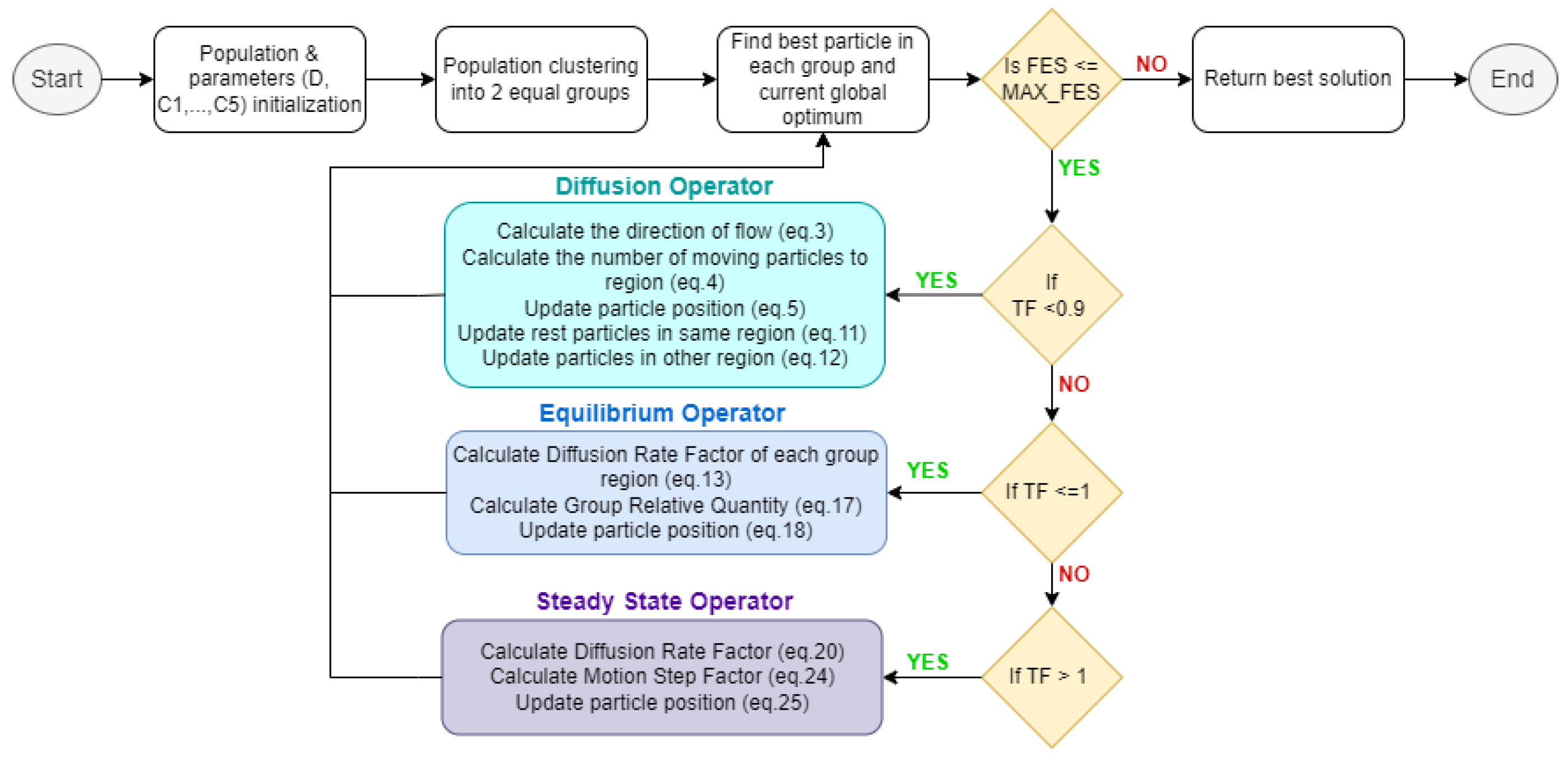
Figure 2.
Flowchart of FLA-OBL.
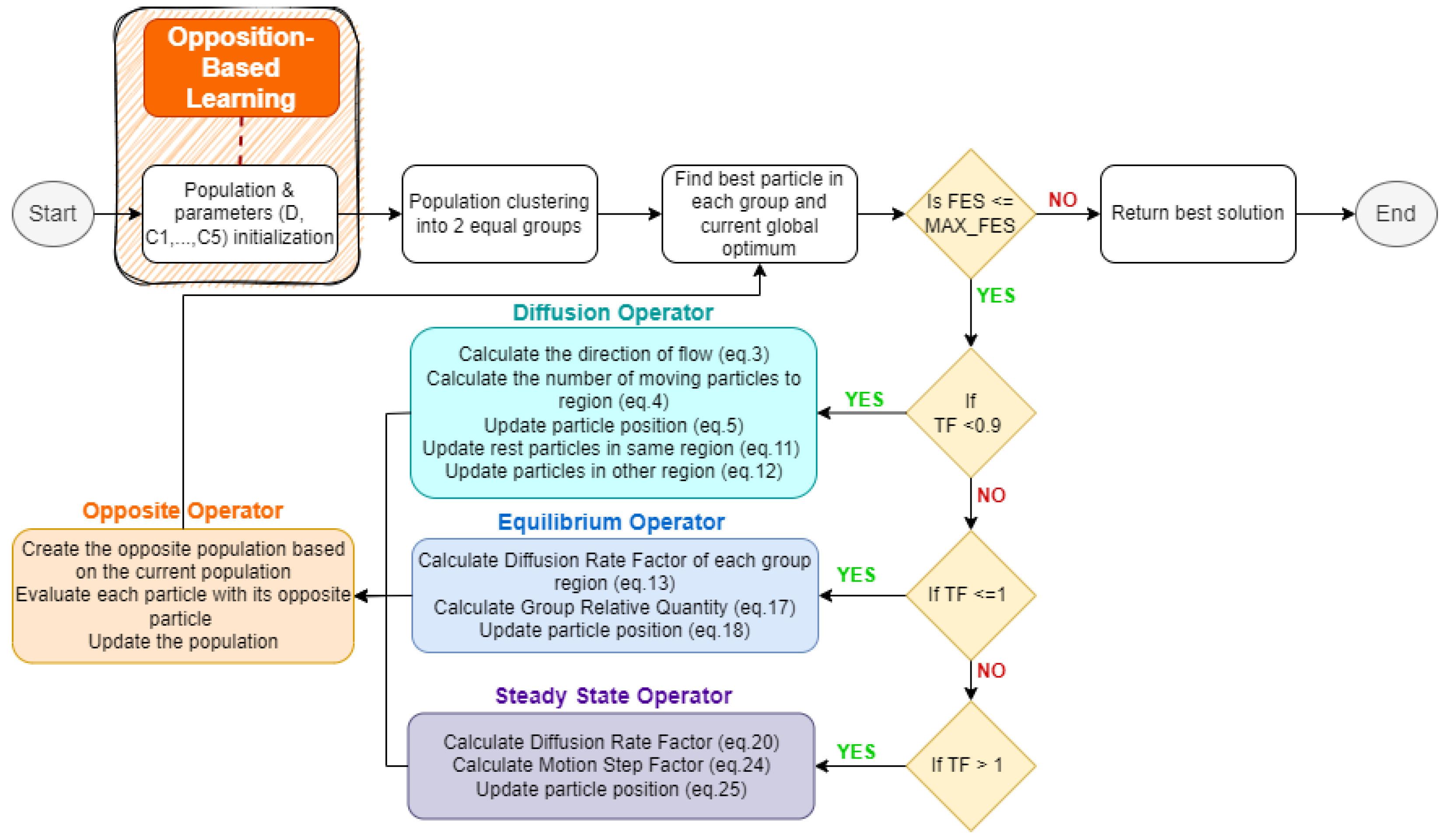
Figure 3.
Flowchart of FFLA-OBL.
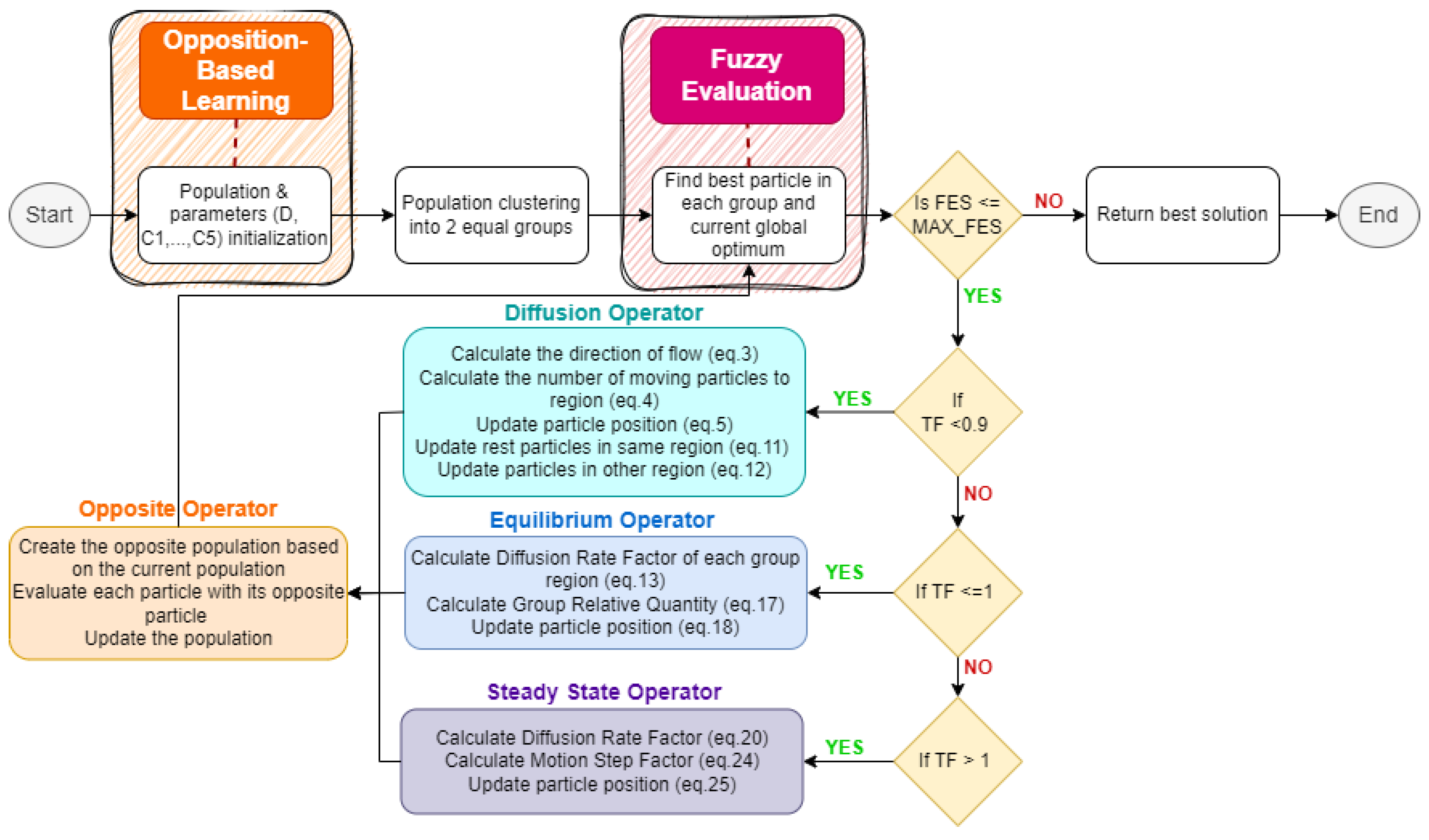
Figure 5.
Membership function of objective term Traveled Distance (Equation (29)).
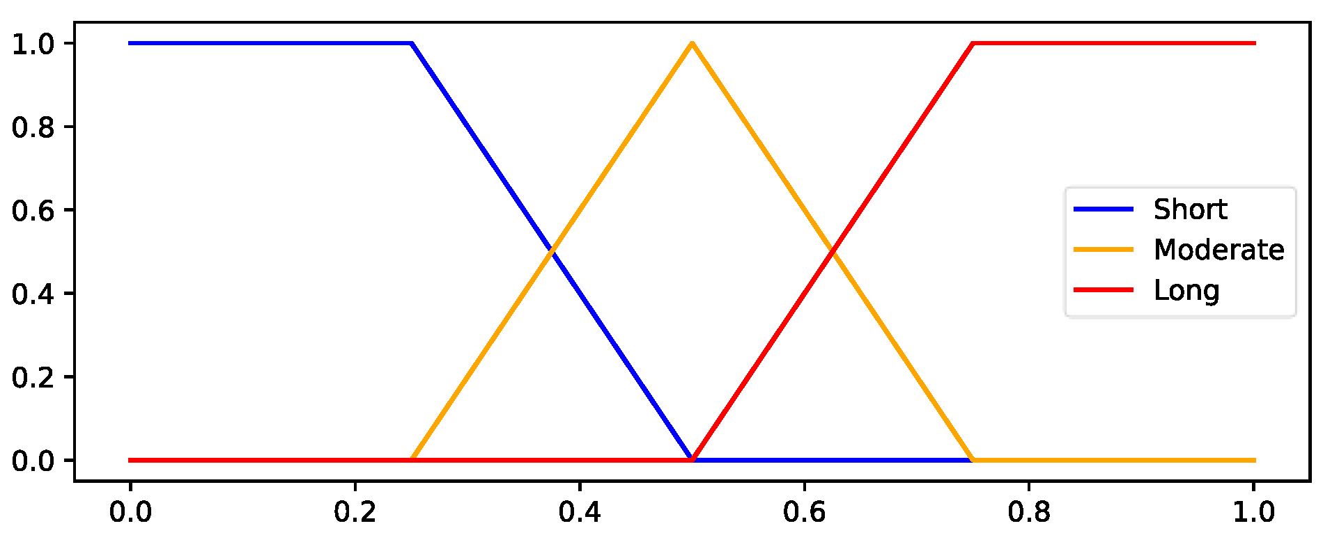
Figure 6.
Membership function of objective term Path Curvature (Equation (30)).
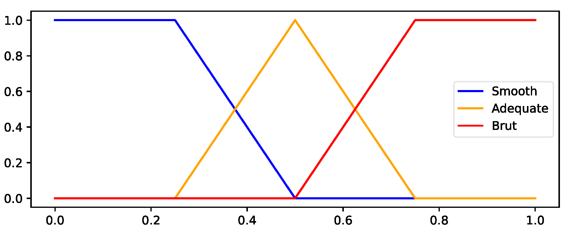
Figure 7.
Membership function of objective term Collision Risk (Equation (33)).
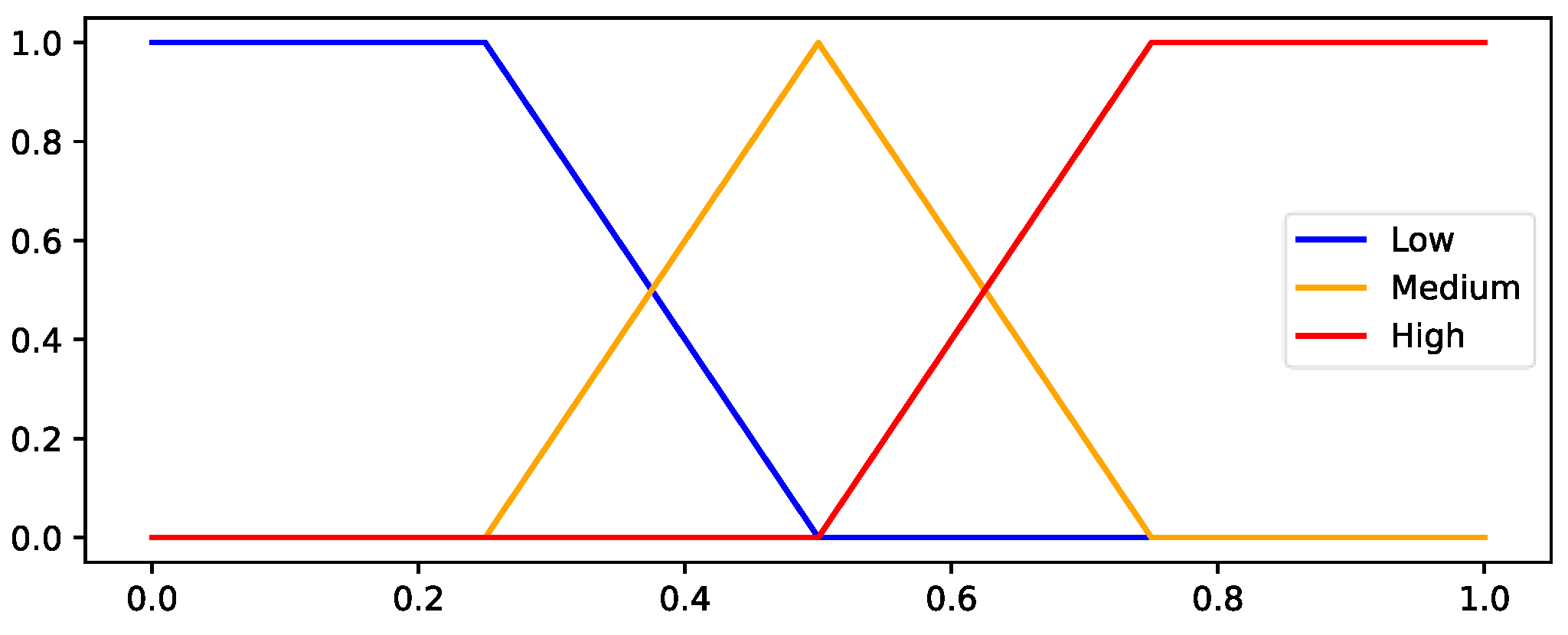
Figure 8.
Membership function of Path Quality.
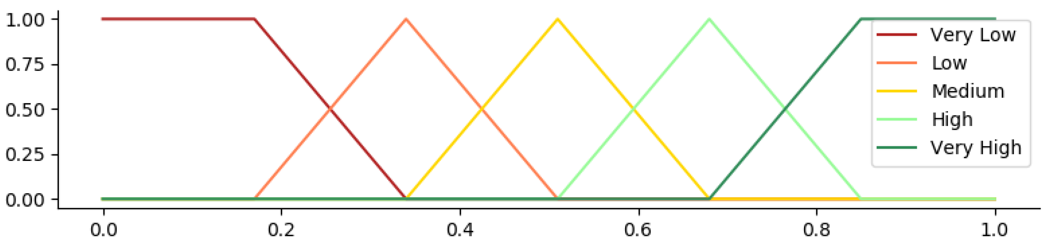
Figure 9.
Flowchart of Fuzzy Evaluation process.
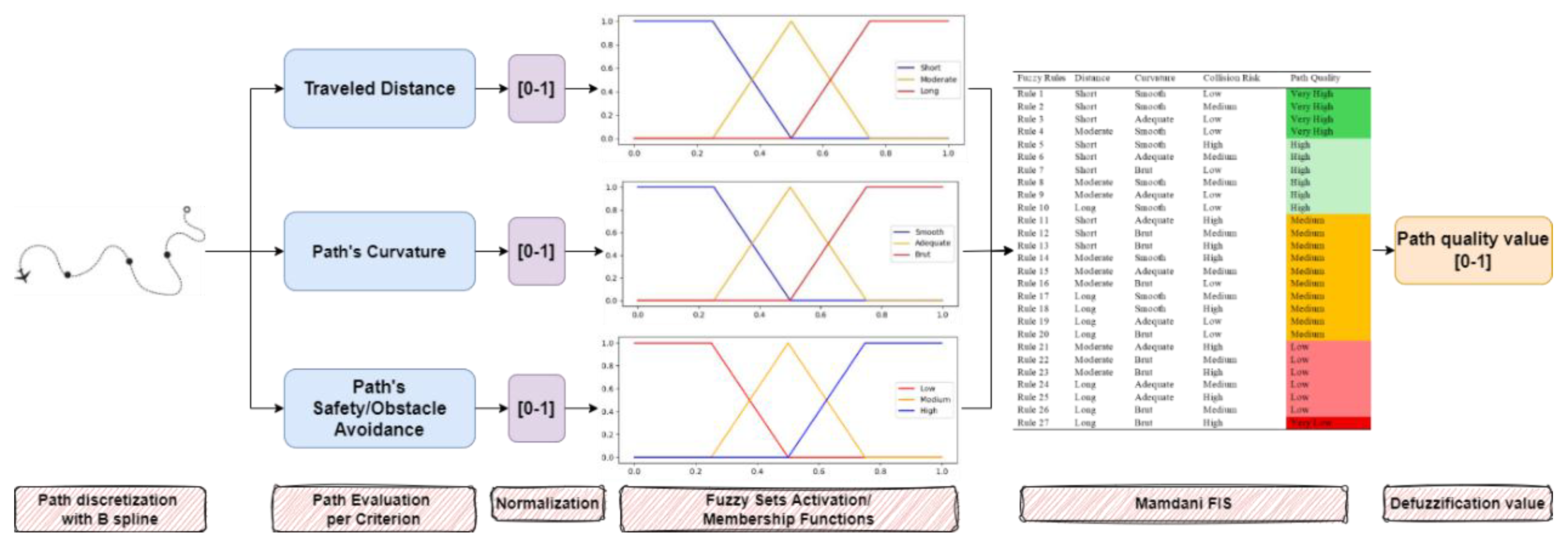
Figure 10.
Ranking of each algorithm for the unimodal, the multimodal, the hybrid, and the composition functions of CEC2017, and overall.
Figure 10.
Ranking of each algorithm for the unimodal, the multimodal, the hybrid, and the composition functions of CEC2017, and overall.
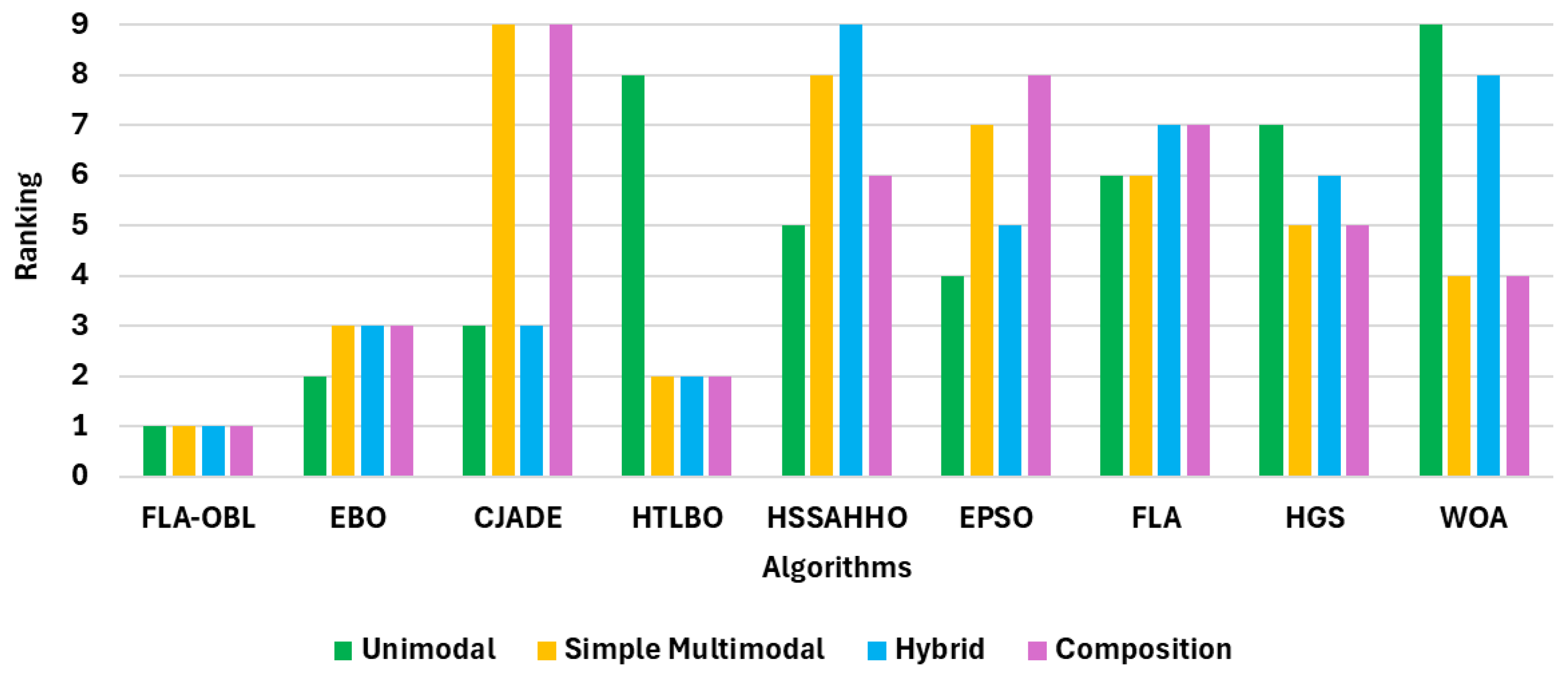

Table 1.
Fuzzy rules of FIS.
| Fuzzy Rules | Distance | Curvature | Collision Risk | Path Quality |
| Rule 1 | Short | Smooth | Low | Very High |
| Rule 2 | Short | Smooth | Medium | Very High |
| Rule 3 | Short | Adequate | Low | Very High |
| Rule 4 | Moderate | Smooth | Low | Very High |
| Rule 5 | Short | Smooth | High | High |
| Rule 6 | Short | Adequate | Medium | High |
| Rule 7 | Short | Brut | Low | High |
| Rule 8 | Moderate | Smooth | Medium | High |
| Rule 9 | Moderate | Adequate | Low | High |
| Rule 10 | Long | Smooth | Low | High |
| Rule 11 | Short | Adequate | High | Medium |
| Rule 12 | Short | Brut | Medium | Medium |
| Rule 13 | Short | Brut | High | Medium |
| Rule 14 | Moderate | Smooth | High | Medium |
| Rule 15 | Moderate | Adequate | Medium | Medium |
| Rule 16 | Moderate | Brut | Low | Medium |
| Rule 17 | Long | Smooth | Medium | Medium |
| Rule 18 | Long | Smooth | High | Medium |
| Rule 19 | Long | Adequate | Low | Medium |
| Rule 20 | Long | Brut | Low | Medium |
| Rule 21 | Moderate | Adequate | High | Low |
| Rule 22 | Moderate | Brut | Medium | Low |
| Rule 23 | Moderate | Brut | High | Low |
| Rule 24 | Long | Adequate | Medium | Low |
| Rule 25 | Long | Adequate | High | Low |
| Rule 26 | Long | Brut | Medium | Low |
| Rule 27 | Long | Brut | High | Very Low |
Table 2.
Summary of algorithms used for comparison.
| Algorithm | Year | Category | Source |
| CJADE | 2021 | Hybrid DE/Physics-Inspired | [25] |
| HSSAHHO | 2022 | Hybrid swarm intelligence/Nature-Inspired | [26] |
| EPSO | 2017 | Nature-Inspired | [27] |
| FLA | 2023 | Physics-Inspired | [13] |
| HGS | 2021 | Swarm intelligence with stochastic elements | [24] |
| WOA | 2016 | Nature-Inspired | [28] |
| EBO | 2023 | Hybrid swarm intelligence/ Physics-Inspired | [29] |
| HTBLO | 2021 | Other hybrid learning algorithm | [30] |
Table 3.
Comparative results on the CEC2017 benchmark suite. The symbols and indicate that FLA-OBL performs significantly better, worse, or shows no significant difference, respectively, compared to the competing algorithm, based on the Mann–Whitney U test. An asterisk denotes statistical significance at the level (i.e., ).
| Algorithms | ||||||||||
| Function | FLA-OBL | EBO | CJADE | HTLBO | HSSAHHO | EPSO | FLA | HGS | WOA | |
| F1 | Mean Std MWU Rank |
1.37E+02 6.76E+01 1 |
1.74E+02 1.85E+02 2 |
1.48E−14 3.98E−15 3 |
3.22E+03 3.70E+03 8 |
3.03E+05 1.20E+08 5 |
4.57E+02 5.98E+02 4 |
3.61E+03 4.60E+03 6 |
7.04+03 4.85E+03 7 |
2.29E+06 1.45E+06 9 |
| F3 | Mean Std MWU Rank |
2.17E+02 1.48E+02 2 |
3.94E+02 3.22E+02 4 |
4.52E+03 1.26E+04 8 |
3.00E+02 2.50E-05 1 |
1.02E+03 1.54E+03 7 |
4.68E−08 1.27E−07 5 |
2.17E+02 1.73E+02 3 |
9.01E+02 2.87E+03 6 |
1.36E+05 6.08E+04 9 |
| F4 | Mean Std MWU Rank |
4.54E+02 2.97E+01 1 |
4.59E+02 1.99E+01 2 |
3.96E+01 2.90E+01 8 |
4.62E+02 3.19E+01 3 |
5.39E+02 1.01E+01 4 |
3.17E+01 3.20E+01 9 |
9.34E+01 2.54E+01 6 |
8.94E+01 2.49E+01 7 |
1.40E+02 3.38E+01 5 |
| F5 | Mean Std MWU Rank |
3.71E+02 2.17E+01 3 |
6.04E+02 3.15E+01 1 |
2.59E+01 3.85E+00 8 |
6.07E+02 2.01+01 2 |
1.28E+01 7.43E+00 9 |
5.20E+01 1.19E+01 6 |
4.32E+01 1.17E+01 7 |
1.12E+02 3.12E+01 5 |
2.40E+02 5.05E+01 4 |
| F6 | Mean Std MWU Rank |
6.32E+02 5.33E+00 2 |
6.46E+02 7.35E+00 3 |
1.18E−13 2.23E−14 9 |
6.19E+02 6.17E+00 1 |
1.02E+03 1.98E+02 5 |
1.93E−08 1.01E−07 8 |
7.82E-03 2.13E-03 7 |
5.46E-01 7.37E-01 6 |
6.53E+01 1.03E+01 4 |
| F7 | Mean Std MWU Rank |
8.77E+02 8.10E+01 1 |
9.45E+02 7.80E+01 4 |
5.49E+01 4.05E+00 9 |
8.91E+02 4.80E+02 2 |
1.01E+03 4.72E+01 5 |
9.45E+01 1.41E+01 7 |
7.81E+01 1.16E+01 8 |
1.64E+02 4.28E+01 6 |
4.99E+02 1.06E+02 3 |
| F8 | Mean Std MWU Rank |
8.70E+02 1.24E+01 1 |
8.95E+02 1.58E+01 3 |
2.60E+01 3.78E+00 7 |
8.81E+02 1.64E+02 2 |
6.26E+03 1.19E+03 9 |
5.61E+01 1.55E+01 6 |
4.15E+01 1.13E+01 8 |
1.04E+02 1.70E+01 5 |
2.16E+02 4.28E+01 4 |
| F9 | Mean Std MWU Rank |
1.09E+03 3.14E+02 1 |
1.43E+03 7.96E+02 2 |
1.76E-03 1.25E-02 6 |
1.74E+02 3.34E+02 3 |
6.96E+03 2.19E+03 9 |
7.61E+01 4.39E+01 4 |
3.28E+00 5.55E+00 5 |
2.68E+03 9.66E+02 7 |
6.56E+03 2.36E+03 8 |
| F10 | Mean Std MWU Rank |
2.64E+03 5.52E+02 5 |
4.56E+03 5.73E+02 6 |
1.92E+03 2.54E+02 2 |
4.74E+02 7.85E+02 1 |
1.14E+05 8.85E+04 9 |
5.23E+03 3.34E+02 8 |
2.62E+03 5.22E+02 4 |
2.55E+03 4.81E+02 3 |
4.89E+03 7.76E+02 7 |
| F11 | Mean Std MWU Rank |
1.20E+03 1.85E+01 1 |
1.35E+03 4.05E+01 2 |
3.16E+01 2.57+E01 8 |
1.26E+02 5.15E+01 4 |
1.44E+09 3.56E+10 9 |
5.86E+01 2.87E+01 6 |
3.41E+01 2.84E+01 7 |
1.18E+02 3.00E+01 5 |
3.86E+02 9.75E+01 3 |
| F12 | Mean Std MWU Rank |
2.91E+04 1.30E+04 4 |
1.41E+06 8.30E+05 7 |
1.37E+03 9.43E+02 1 |
2.17E+04 1.43E+04 2 |
3.32E+09 5.04E+09 9 |
2.86E+04 1.37E+04 3 |
5.61E+05 5.01E+05 5 |
9.30E+05 7.21E+05 6 |
4.19E+07 2.95E+07 8 |
| F13 | Mean Std MWU Rank |
1.97E+03 1.31E+03 2 |
2.31E+04 2.75E+04 4 |
4.80E+01 3.27E+01 3 |
9.33E+03 9.62E+03 5 |
4.98E+06 3.77E+07 9 |
1.09E+03 1.07E+03 1 |
1.24E+04 1.22E+04 6 |
3.16E+04 2.54E+04 7 |
1.54E+05 8.71E+04 8 |
| F14 | Mean Std MWU Rank |
4.85+03 2.35E+03 4 |
3.73E+03 4.20E+03 3 |
2.73E+03 5.19E+03 2 |
1.54E+03 4.49E+02 1 |
1.50E+09 1.21E+09 9 |
5.95E+03 8.67E+03 5 |
1.03E+04 1.49E+04 6 |
5.45E+04 4.29E+04 7 |
8.10E+05 8.21E+05 8 |
| F15 | Mean Std MWU Rank |
1.79E+03 1.43E+03 1 |
1.92E+03 1.61E+03 2 |
1.79E+02 1.02E+03 5 |
1.94E+03 2.75E+02 3 |
8.24E+03 4.21E+03 7 |
5.47E+02 6.97E+02 4 |
5.49E+03 7.03E+03 6 |
1.90E+04 1.63E+04 8 |
7.65E+04 5.17E+04 9 |
| F16 | Mean Std MWU Rank |
1.08E+03 3.75E+02 1 |
2.87E+03 2.27E+02 7 |
4.57E+02 1.59E+02 5 |
2.87E+03 2.43E+02 8 |
4.06E+04 1.27E+06 9 |
6.38E+02 2.13E+02 4 |
3.71E+02 1.59E+02 6 |
1.06E+03 3.74E+02 2 |
1.87E+03 4.15E+02 3 |
| F17 | Mean Std MWU Rank |
1.86+03 1.08E+02 1 |
1.91E+03 1.13E+02 2 |
7.42E+01 2.67E+01 8 |
1.92E+03 9.40E+02 3 |
1.24E+07 5.13E+07 9 |
1.99E+02 1.04E+02 6 |
1.22E+02 6.87E+01 7 |
4.64E+02 1.62E+02 5 |
8.58E+02 2.87E+02 4 |
| F18 | Mean Std MWU Rank |
2.48E+03 3.72E+04 1 |
3.32E+03 2.25E+04 2 |
6.72E+03 3.52E+04 4 |
3.77E+03 2.18E+02 3 |
1.53E+08 6.09E+08 9 |
1.04E+05 8.99E+04 5 |
1.71E+05 1.39E+05 6 |
2.40E+05 2.17E+05 7 |
2.79E+06 2.17E+06 8 |
| F19 | Mean Std MWU Rank |
6.39E+02 2.04E+03 4 |
1.25E+05 8.04E+04 8 |
3.05E+02 2.02E+03 5 |
2.12E+03 1.04E+02 2 |
2.01E+03 4.99E+01 1 |
8.23E+02 1.46E+03 3 |
9.52E+03 1.05E+04 7 |
1.81E+04 2.05E+04 6 |
2.31E+06 2.15E+06 9 |
| F20 | Mean Std Rank |
2.12E+03 1.08E+02 1 |
2.21E+03 1.05E+02 2 |
1.14E+02 5.43E+01 9 |
2.24E+03 8.36E+01 3 |
3.050E+03 8.21E+01 4 |
2.18E+02 1.27E+02 7 |
1.62E+02 8.01E+01 8 |
4.83E+02 1.62E+02 6 |
7.14E+02 2.08E+02 5 |
| F21 | Mean Std MWU Rank |
2.54E+03 1.06E+01 1 |
2.95E+03 8.49E+01 3 |
2.26E+02 3.97E+00 8 |
2.59E+03 1.81E+01 2 |
2.18E+04 1.66E+03 9 |
2.54E+02 3.09E+01 6 |
2.44E+02 1.12E+01 7 |
3.19E+02 3.60E+01 5 |
4.54E+02 6.92E+01 4 |
| F22 | Mean Std MWU Rank |
3.60E+03 1.15E+03 3 |
5.80E+03 1.74E+03 9 |
1.00E+02 1.00E−13 7 |
2.38E+03 5.63E+02 1 |
4.11E+03 1.38E+02 4 |
1.42E+02 2.99E+02 5 |
1.01E+02 1.39E+00 6 |
2.97E+03 8.91E+02 2 |
4.37E+03 1.97E+03 8 |
| F23 | Mean Std MWU Rank |
2.49E+03 3.43E+01 2 |
2.77E+03 8.29E+01 3 |
3.73E+02 5.24E+00 9 |
2.79E+03 5.07E+01 4 |
2.38E+03 7.61E+01 1 |
4.09E+02 1.44E+01 7 |
3.95E+02 1.19E+01 8 |
4.59E+02 2.23E+01 6 |
7.52E+02 9.65E+01 5 |
| F24 | Mean Std Rank |
2.66E+03 3.73E+01 1 |
2.93E+03 5.38E+01 2 |
4.42E+02 4.76E+00 7 |
2.94E+03 4.21E+01 3 |
1.24E+04 1.06E+04 9 |
4.81E+025.76E+01 6 |
4.61E-02 1.54E+01 8 |
5.95E+02 5.37E+01 5 |
7.70E+02 8.25E+01 4 |
| F25 | Mean Std MWU Rank |
2.74E+03 1.34E+01 1 |
2.89E+03 1.06E+01 2 |
3.87E+02 5.35E-01 6 |
2.90E+03 1.96E+01 3 |
2.06E+04 2.45E+03 8 |
3.87E+02 1.61E+00 7 |
3.93E+02 1.16E+01 5 |
3.87E+02 2.53E+00 9 |
4.46E+02 3.15E+01 4 |
| F26 | Mean Std MWU Rank |
1.22E+03 8.22E+03 4 |
6.27E+03 1.52E+03 9 |
1.20E+03 8.20E+01 3 |
4.61E+03 1.14E+03 8 |
4.09E+03 1.09E+03 5 |
7.23E+02 7.03E+02 6 |
1.55E+03 2.35E+02 2 |
2.19E+03 5.72E+02 1 |
4.57E+03 1.21E+03 7 |
| F27 | Mean Std MWU Rank |
3.01E+03 2.08E+01 3 |
3.22E+03 1.95E+01 1 |
5.04E+02 8.10E+00 8 |
3.25E+03 3.82E+01 2 |
6.13E+03 4.83E+01 9 |
5.16E+02 8.72E+00 6 |
5.08E+02 5.62E+00 7 |
5.24E+02 1.30E+01 5 |
6.72E+02 1.04E+02 4 |
| F28 | Mean Std MWU Rank |
2.91E+03 1.75E+01 1 |
3.14E+03 2.37E+01 2 |
3.34E+02 5.50E+01 8 |
3.47E+03 5.75E+01 4 |
3.42E+03 1.42E+01 3 |
3.31E+02 5.10E+01 9 |
4.81E+02 2.26E+01 6 |
4.12E+02 3.91E+01 7 |
4.94E+02 2.21E+01 5 |
| F29 | Mean Std MWU Rank |
3.65E+03 1.04E+02 2 |
3.70E+03 1.95E+02 3 |
4.78E+02 2.32E+01 8 |
3.64E+03 1.67E+02 1 |
3.04E+05 4.68E+04 9 |
6.12E+02 8.88E+01 6 |
5.45E+02 9.28E+01 7 |
8.62E+02 1.97E+02 5 |
1.80E+03 3.80E+02 4 |
| Total ranking | 1 | 3 | 8 | 2 | 9 | 5 | 7 | 6 | 4 | |
| Total MWU | 22/2/3 | 24/1/3 | 15/4/9 | 25/0/3 | 25/1/2 | 25/2/1 | 24/2/2 | 28/0/0 | ||
Table 4.
Results of Friedman test per function categories of CEC2017.
| Functions | ||||||
| all | Unimodal | Multimodal | Hybrid | Composition | ||
| p-value | 9.01E-22 | 2.14E-03 | 1.95E-03 | 4.64E-07 | 4.24E-10 | |
| Chi-square | 117.90 | 25.57 | 24.42 | 44.47 | 60.21 | |
Table 5.
Convergence and DFLA mean results on functions of CEC2017.
| Algorithms | |||||
| Function | Metrics | FLA-OBL | EBO | HTLBO | FLA |
| F1 | EQG EC EVP |
0.36 0.48 0.77 |
0.37 0.45 0.64 |
2.46E-03 2.23E-03 0.23 |
1.76E-03 2.08E-03 0.28 |
| F5 | EQG EC EVP |
0.34 0.37 0.66 |
0.40 0.49 0.71 |
0.38 0.46 0.70 |
9.13E-02 9.28E-02 0.31 |
| F7 | EQG EC EVP |
0.38 0.47 0.71 |
0.27 0.31 0.52 |
0.35 0.43 0.69 |
2.05E-03 2.41E-03 0.21 |
| F16 | EQG EC EVP |
0.33 0.47 0.62 |
2.25E-03 2.42E-03 0.23 |
1.05E-03 1.68E-03 0.19 |
9.46E-02 9.84E-02 0.28 |
| F19 | EQG EC EVP |
0.28 0.36 0.53 |
2.34E-03 2.76E-03 0.21 |
0.38 0.44 0.74 |
3.66E-03 3.87E-03 0.22 |
| F21 | EQG EC EVP |
0.44 0.48 0.73 |
0.39 0.42 0.62 |
0.41 0.47 0.68 |
9.38E-02 9.41E-02 0.25 |
| F26 | EQG EC EVP |
0.29 0.38 0.57 |
6.23E-02 6.56E-02 0.20 |
9.32E-02 9.84E-02 0.22 |
0.46 0.51 0.73 |
| Total Average | EQG EC EVP |
0.35 0.43 0.66 |
0.21 0.25 0.45 |
0.23 0.27 0.49 |
0.11 0.12 0.33 |
Table 6.
Results of FLA and FFLA-OBL for 3 UAV path planning scenarios with increasing complexity.
| Scenarios | Evaluation criteria | FLA | FFLA-OBL |
| Scenario 1 (7 obstacles) |
Traveled distance Path deviations Penalty (collision risk) Path quality RPD (%) |
13.64 5 0.11 0.75 15 |
10.97 3 0 0.88 0 |
| Scenario 2 (12 obstacles) |
Traveled distance Path deviations Penalty (collision risk) Path quality RPD (%) |
15.72 3 0.46 0.62 23 |
11.73 3 0.08 0.77 0 |
| Scenario 3 (18 obstacles) |
Traveled distance Path deviations Penalty (collision risk) Path quality RPD (%) |
16.43 8 0.37 0.52 27 |
13.89 4 0 0.71 0 |
Disclaimer/Publisher’s Note: The statements, opinions and data contained in all publications are solely those of the individual author(s) and contributor(s) and not of MDPI and/or the editor(s). MDPI and/or the editor(s) disclaim responsibility for any injury to people or property resulting from any ideas, methods, instructions or products referred to in the content. |
© 2025 by the authors. Licensee MDPI, Basel, Switzerland. This article is an open access article distributed under the terms and conditions of the Creative Commons Attribution (CC BY) license (http://creativecommons.org/licenses/by/4.0/).
Copyright: This open access article is published under a Creative Commons CC BY 4.0 license, which permit the free download, distribution, and reuse, provided that the author and preprint are cited in any reuse.


