
Submitted:
08 July 2025
Posted:
11 July 2025
You are already at the latest version
Abstract
Forecasting over dynamic graph environments necessitates modeling both long-term temporal dependencies and evolving structural patterns. We propose MaGNet BN, a modular framework that simultaneously performs probabilistic forecasting and dynamic community detection on temporal graphs. MaGNet BN integrates Bayesian node embeddings for uncertainty modeling, prototype guided Louvain clustering for community discovery, Markov based transition modeling to preserve temporal continuity, and reinforcement based refinement to improve structural boundary accuracy. We evaluate MaGNet-BN on real world datasets in pedestrian mobility, energy consumption, and retail demand. Experimental results show that our model consistently outperforms state of the art baselines in predictive accuracy (MSE, NLL, CRPS), uncertainty calibration (PICP), and structural coherence (Modularity, tARI). Ablation studies highlight the complementary strengths of each component. Overall, MaGNet BN delivers a structure aware and uncertainty calibrated forecasting system that models both temporal evolution and dynamic community formation. Its modular design enables interpretable predictions and scalable application across smart cities, energy systems, and personalized services.
Keywords:
Temporal Graph Forecasting
; Dynamic Community Detection
; Bayesian Graph 16 Neural Networks
; Uncertainty Calibration
; Markov Modeling
; Reinforcement Learning
1. Introduction
Forecasting pedestrian flows, electricity demand, and retail sales in dynamic environments necessitates models capable of managing both long-term temporal patterns and continually evolving interaction graphs [12,29]. Each time step can be conceptualized as a graph in which node clusters (communities) fluctuate in accordance with behavioral trends and seasonal influences[19].
Most current forecasters presume a fixed graph topology [10,21] or static spatial priors [12], neglecting to explicitly account for uncertainty—an imperative consideration in safety-critical sectors such as energy forecasting and retail planning. Dynamic community identification approaches seek to identify developing network structures; however, they frequently analyze temporal snapshots in isolation or utilize heuristic smoothing, resulting in the omission of nuanced structural transitions [1].
Despite recent advancements, the concurrent modeling of dynamic signals and developing graph structures continues to pose significant challenges. Real-world graphs, including transportation networks, social interactions, and energy systems, frequently experience sudden topological changes due to external events or seasonal patterns. Conventional GNN-based forecasts are constrained by static or gradually adjusting adjacency assumptions, which inadequately reflect rapid structural changes. Community detection approaches frequently exhibit insufficient predictive powers and depend on heuristic post-processing, rendering them inappropriate for real-time forecasting applications. This disparity underscores the necessity for a cohesive framework capable of both forecasting long-term signal patterns and meticulously monitoring underlying structural changes.
To overcome these restrictions, we present MaGNet-BN, a cohesive framework that simultaneously executes long-term forecasting and dynamic community monitoring on temporal graphs. The model comprises four synergistic elements: (i) a Bayesian node embedding module that encapsulates epistemic uncertainty; (ii) a prototype-guided Louvain clustering strategy that yields interpretable and temporally consistent communities; (iii) a Markov smoothing mechanism that simulates community evolution through merging or splitting; and (iv) a reinforcement learning-based refinement phase utilizing PPO, which adaptively reallocates boundary nodes according to a learnable reward function, thereby obviating the necessity for manually crafted heuristics.
1.1. Contributions
Unified probabilistic framework — MaGNet-BN is the first end-to-end model that jointly performs calibrated long-horizon forecasting and dynamic community tracking. It fuses Bayesian node embeddings, prototype-guided Louvain clustering, Markov smoothing, and PPO refinement into a single, differentiable pipeline.
New state-of-the-art on seven datasets — Across traffic, mobility, social, e-mail, energy, and retail domains, MaGNet-BN tops 26 / 28 forecasting scores (MSE, NLL, CRPS, PICP) and every structural metric (Q, tARI, NMI), outperforming seven strong baselines.
Efficiency & robustness — A complete hyper-parameter sweep plus training finishes in 11 GPU-hours on one A100. Worst-case MSE drift under parameter sweeps is < 2.7 %, and modularity drop under 5 % edge-rewiring is halved versus the best dynamic-GNN baseline.
Reproducible research assets — We provide sanitized datasets, code, and a cohesive assessment workflow, thereby establishing a replicable standard for probabilistic forecasting in the context of dynamic community evolution.
2. Related Work
Our research intersects three essential domains: temporal graph forecasting, dynamic community recognition, and uncertainty-aware graph learning. We examine exemplary work in each subject and emphasize the unique aspects of our suggested methodology.
2.1. Temporal Graph Forecasting
Temporal graph forecasting emphasizes the modeling of time-varying signals inside graph-structured data. Traditional methodologies, including DCRNN [12], TGCN [2], and Graph WaveNet [4], integrate graph convolutional networks with recurrent neural networks to effectively capture spatial and temporal dependencies. Transformer-based approaches, such as Informer [24] and TFT [10], prioritize long-range temporal modeling using attention mechanisms, however predominantly presuppose static topologies and immutable graph structures.
Recent endeavors have sought to tackle dynamicity. Huang and Lei [5] present group-aware graph diffusion for dynamic link prediction. Nonetheless, their methodology does not explicitly account for community change or uncertainty. Conversely, our suggested MaGNet-BN architecture incorporates dynamic community tracking into the forecasting process, facilitating structure-aware long-term prediction.
2.2. Dynamic Community Detection
Dynamic community detection aims to identify and monitor the evolution of node clusters over time. Current methodologies generally execute snapshot-level clustering autonomously [19] or utilize heuristic temporal smoothing [1], potentially leading to inconsistent or imprecise results. Reinforcement-based methodologies, exemplified by Costa et al. [6], have enhanced modularity-driven clustering through the acquisition of dynamic policies; nevertheless, they do not integrate temporal forecasting.
MaGNet-BN addresses this disparity by concurrently simulating community dynamics and sequence prediction using a Markovian transition process, augmented with reinforcement-based structural optimization.
2.3. Uncertainty-Aware Graph Learning
Bayesian Neural Networks (BNNs) and methods such as Monte Carlo dropout have been utilized to assess epistemic uncertainty in node-level and predictive tasks. Pang et al. [17] employ Bayesian spatio-temporal transformers for trajectory prediction, providing uncertainty-aware modeling. Nevertheless, these methodologies frequently overlook the significance of dynamic graph topologies or communities.
Our research advances this area by integrating uncertainty at both the embedding level and the community building process. This facilitates strong, comprehensible predictions with structural insight and probabilistic assurance.
3. Methodology
This section presents MaGNet-BN, a modular framework aimed at achieving calibrated forecasting and reliable structural tracking in dynamic graphs. The framework consists of five successive modules, each designated for a specific learning aim.
3.1. Pipeline Overview
MaGNet-BN operates through five stages: (1) preprocessing input sequences into temporal graphs, (2) extracting Bayesian node embeddings, (3) deriving initial communities via prototype-guided Louvain clustering, (4) estimating Markov transitions between communities, and (5) refining boundaries using PPO reinforcement. Figure 1 provides a comprehensive overview.
Figure 1.
Illustration of the MaGNet-BN pipeline. The model processes temporal graph snapshots in five stages: (1) data preprocessing generates clean snapshot graphs; (2) Bayesian node embeddings are computed via variational inference; (3) k-NN graph and prototype-guided Louvain clustering yield initial communities ; (4) Markov transitions capture inter-snapshot dynamics; (5) a PPO agent refines community assignments to produce .
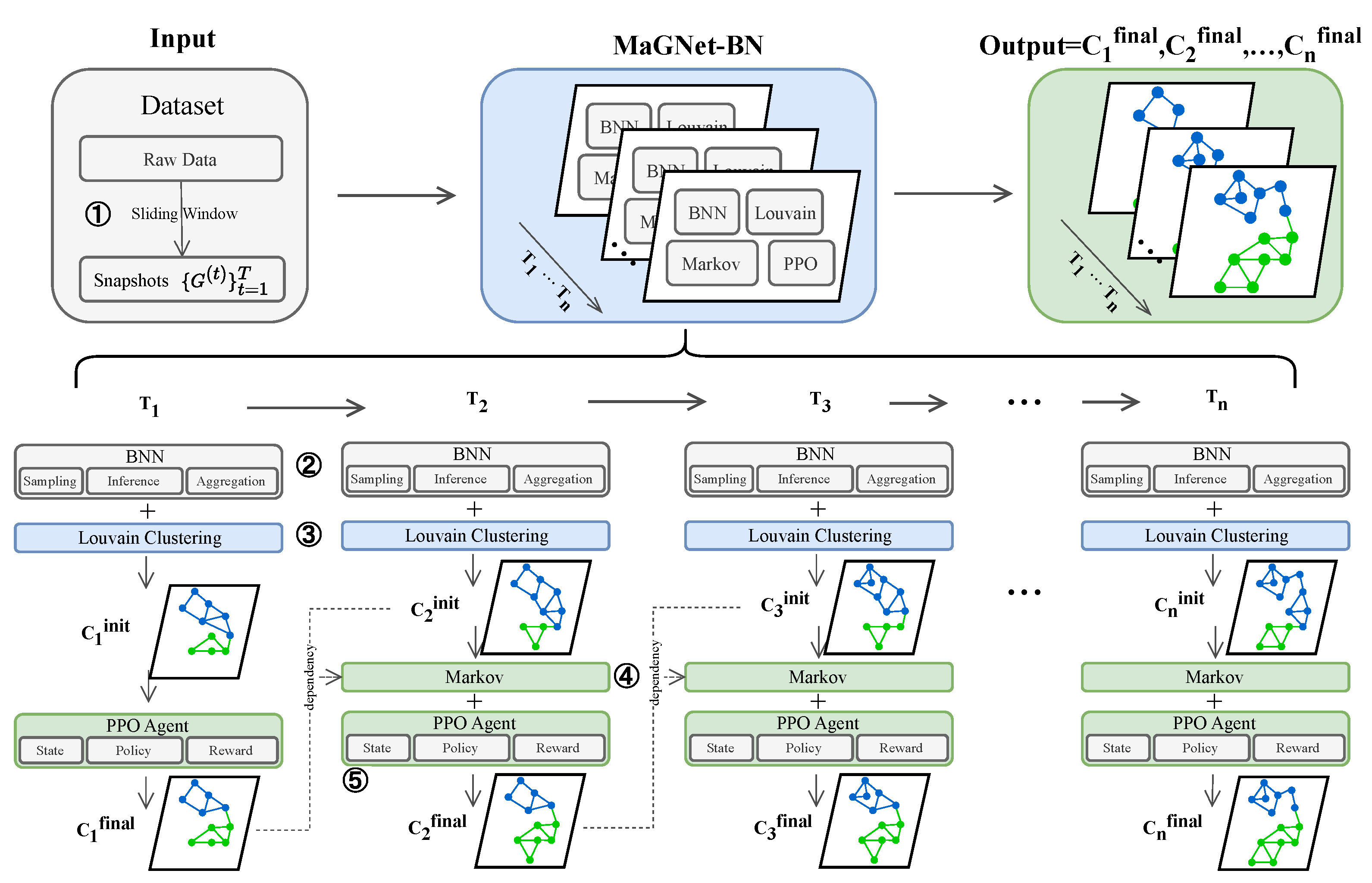
We now describe each component in detail, starting with the data preprocessing step.
3.2. Data Preprocessing
Given a sequence of observations , we apply a sliding window of length L and stride to generate a series of T overlapping snapshots. Each window defines a graph , where nodes and edges are constructed from temporal interactions or spatial relations within the window.
Continuous characteristics undergo Z-score normalization, whilst categorical features are converted into dense vectors by learnt embeddings. To address missing values, we utilize a hybrid imputation approach that integrates forward-fill and k-nearest neighbor interpolation. The resultant node attribute matrix functions as input to the Bayesian embedding layer.
While we utilize k-NN graphs on latent embeddings to establish edges, this procedure is heuristic and remains static once created. This may potentially introduce edge noise or improper structural assumptions. More formally, for each node v, its neighborhood is selected as:
This method disregards feedback from downstream task performance while selecting edges. A viable alternative is Graph Structure Learning (GSL) [15,16], in which the adjacency matrix is concurrently learnt with node representations. This adaptive modeling could enhance forecast precision and structural coherence.
Finally, MaGNet-BN presumes that node features are either numerical or categorical and does not presently accommodate multimodal inputs, including text, photos, or geospatial data. Future enhancements may integrate pretrained encoders [9] or transformer-based fusion models [13] to facilitate wider applicability in fields encompassing multimodal sensor data, documents, or videos.
3.3. Bayesian Embedding
To capture uncertainty in node representations, we adopt a Bayesian neural network (BNN), where the weights of the GNN are modeled as Gaussian distributions with variational parameters:
sampled using the reparameterization trick: , with .
The BNN is trained by maximizing the evidence lower bound (ELBO) [14]:
Each node embedding is estimated by averaging over M Monte Carlo samples:
3.4. Prototype-Guided Louvain Clustering
To derive initial community assignments , we construct a sparse k-nearest neighbor graph using the node embeddings through cosine similarity. Thereafter, we employ the Louvain algorithm [3] to enhance modularity on , yielding superior clustering partitions.
To enable temporal synchronization, we additionally produce P representative nodes for each community based on distinct PageRank scores. These high-centrality nodes function as enduring structural anchors and provide consistent references for the Markov and reinforcing phases. We select prototypes via personalized PageRank:
where denotes the normalized transition matrix and represents the teleport parameter. This approach effectively emphasizes central nodes but may prioritize high-degree hubs, neglecting architecturally significant yet peripheral nodes. To mitigate this bias, subsequent research could implement diversity-aware selection [36] or entropy-based node selection to encapsulate diverse community roles.
3.5. Markov Transition Modeling
To capture inter-snapshot dynamics, we estimate a community-level transition matrix using a first-order Markov model. Let denote the community assignment of node v at time t. The transition probability from community j at to k at t is computed as:
where is a Laplace smoothing factor. The resulting matrix encourages temporal consistency by penalizing community switches that deviate from dominant transition patterns. Our model estimates first-order transition matrices assuming that structural evolution follows a Markovian process:
This simplification is efficient but may not capture long-term dependencies or delayed effects. Future work may explore higher-order Markov chains [20] or memory-enhanced models like HMMs and RNNs [8], which model transitions with richer histories and dynamic priors.
3.6. Reinforcement-Based Refinement
We frame boundary node reallocation as a reinforcement learning (RL) problem to enhance temporal smoothness and modularity. A boundary node v is characterized by neighbors associated with distinct communities, indicating uncertainty in its classification.
Each node’s state is defined as:
where and are Bayesian embeddings, is the Markov transition vector for v’s current community , and denotes node degree.
The agent selects an action with reward:
which combines modularity gain (), conductance reduction, and Markov-guided transition likelihood. All terms are normalized to .
Policy and value functions are trained via PPO [23], enabling optimization of non-differentiable objectives like modularity while avoiding greedy local minima. The final assignments reflect globally consistent and temporally coherent community structures. While PPO stabilizes updates using the clipped surrogate loss [23], training can still be sensitive to reward scaling and exploration variance:
where is the policy ratio and the advantage estimator. We noted intermittent policy instability when boundary nodes exhibited contradicting modularity and Markov scores. Future enhancements may encompass offline reinforcement learning [11] or curriculum-based policy warming to prevent premature divergence.
3.7. Loss Function & Optimisation
The overall objective combines forecasting fidelity, Bayesian regularisation and structural coherence:
where is mean-squared error (MSE) for deterministic runs or negative log-likelihood (NLL) for probabilistic output; is the evidence lower bound of the Bayesian encoder; enforces community-label continuity; is the clipped surrogate objective used by Proximal Policy Optimisation.
Default weights are selected via grid search on the validation split (range ). Training uses AdamW (, weight-decay ) with a cosine scheduler and early stopping (patience = 20).
3.8. Computational Complexity
Let each snapshot contain nodes and edges ( after k-NN sparsification), d be the hidden size, L the GNN depth, M the Monte-Carlo samples used by the Bayesian encoder, and U the PPO updates applied to B boundary nodes. All results are per epoch over T snapshots.
3.8.1. Bayesian Encoder (dominant)
A sparse GCN layer costs ; M samples and L layers therefore give
3.8.2. Prototype Louvain
Cosine k-NN search plus Louvain modularity adds , sub-linear to the encoder term when .
3.8.3. Markov Update
One pass over node labels: – negligible.
3.8.4. PPO Refinement
Actor–critic MLP () on B boundary nodes for U steps: . In practice ().
3.8.5. Total
3.9. Memory
Main memory stems from M sampled embeddings and PPO buffers: , well within 80GB for the largest dataset.
Hence MaGNet-BN scales linearly with graph size and is practical for mid- to large-scale temporal graphs.
3.10. Algorithm
Algorithm 1 summarises the full training and inference routine. The pipeline proceeds from raw windowed snapshots through five clearly delineated stages: (i) data cleaning, (ii) variational Bayesian node embedding, (iii) prototype-guided Louvain clustering, (iv) Markov smoothing of community trajectories, and (v) PPO-based boundary refinement. This modular decomposition makes each learning signal — likelihood, ELBO, Markov continuity and RL rewards — explicit, enabling stable end-to-end optimisation under the joint loss of Equation (11). At inference time the same sequence of steps (sans gradient updates) yields both calibrated forecasts and temporally coherent community labels , facilitating downstream decision support in dynamic-graph environments.
| Algorithm 1 MaGNet-BN — Unified Training Procedure |
|
4. Evaluation
4.1. Datasets
We evaluate MaGNet-BN on seven publicly available dynamic-graph datasets spanning six real-world domains: traffic (2), mobility, social media, e-mail, energy and retail. Table 1 summarises their statistics.

Table 1.
Statistics of the seven benchmark datasets used in this study. and denote the number of nodes and (average) edges per snapshot; T is the number of temporal snapshots; is the sampling interval.
Table 1.
Statistics of the seven benchmark datasets used in this study. and denote the number of nodes and (average) edges per snapshot; T is the number of temporal snapshots; is the sampling interval.
| Dataset | Domain | (avg) | T | ||
|---|---|---|---|---|---|
| METR–LA | Traffic | 207 | 1 515 | 34 272 | 1 h |
| PeMS–BAY | Traffic | 325 | 2 694 | 52 560 | 1 h |
| TwitterRC | Social | 22 938 | 98 421 | 2 160 | 1 h |
| Enron-Email | 150 028 | 347 653 | 194 | 168 h | |
| ETH+UCY | Mobility | 1 536† | 12 430 | 3 588 | 12 s |
| ELD-2012 | Energy | 370 | 4 862 | 8 760 | 1 h |
| M5-Retail | Retail | 3 049 | 11 216 | 1 941 | 24 h |
† Peak number of distinct pedestrian IDs observed across the ETH + UCY scenes; actual active nodes per snapshot vary between 0–60.
- METR-LA and PeMS-BAY—minute-level road-traffic speeds from loop detectors in Los Angeles and the Bay Area ( and snapshots) [12].
- TwitterRC—2 160 hourly snapshots of retweet/mention interactions among 22 938 users [25].
- Enron-Email—194 weekly snapshots of corporate e-mail exchanges (150 028 nodes) [26].
- ETH+UCY—3 588 twelve-second pedestrian-interaction graphs recorded in public scenes [27].
- ELD-2012—8 760 hourly power-consumption graphs (370 smart-meter clients) extracted from the ElectricityLoadDiagrams20112014 dataset [28].
- M5-Retail—1 941 daily sales-correlation graphs covering 3 049 Walmart items [29].
All datasets are split 70 %/15 %/15 % (train/val/test) in chronological order.
4.2. Baselines
We compare MaGNet-BN with seven representative baselines, carefully chosen to cover the three research threads intertwined in our task—time-series forecasting, dynamic-graph learning, and uncertainty-aware community detection. Table 2 summarises how they span these facets.
4.2.1. Sequence-Forecasting Baselines (Graph-Agnostic)
- DeepAR [21]. Autoregressive LSTM with Gaussian output quantiles; a de-facto standard for univariate/multivariate probabilistic forecasting. Why: sets the reference point for purely temporal models without spatial bias.
- MC-Drop LSTM [7]. Injects dropout at inference to sample from the weight posterior—simple yet strong Bayesian baseline. Why: isolates the benefit of explicit epistemic uncertainty without graph information.
- Temporal Fusion Transformer (TFT) [10]. Multi-head attention, static covariates and gating; current SOTA on many time-series leaderboards. Why: strongest recent non-graph forecaster.
- DCRNN [12]. Diffusion convolution on a fixed sensor adjacency, followed by seq2seq GRU. Why: canonical example of static-graph-aware spatio–temporal forecasting.
4.2.2. Dynamic-Graph Baselines
- DySAT [22]. Self-attention across structural and temporal dimensions; acquires snapshot-specific embeddings. Why: early but influential method; serves as the “attention-without-memory’’ extreme.
- TGAT [18]. Time-encoding kernels plus graph attention, enabling continuous-time message passing. Why: tests whether high-resolution event timing alone suffices for our coarse snapshot setting.
- TGN [25]. Memory modules store node histories and are updated by temporal messages; often SOTA on link prediction. Why: strongest publicly available dynamic-GNN with memory.
All baselines inherit the preprocessing in Section 4.1. Evaluation covers structural coherence (Modularity[34], and temporal ARI[35]) by re-clustering last-layer embeddings with the unified pipeline of §??.
Table 2.
Taxonomy of baselines and the facets they cover.
| Model | Temporal Forecast | Dynamic Graph | Uncertainty / RL |
|---|---|---|---|
| DeepAR | √ | — | Gaussian output |
| MC-Drop LSTM | √ | — | MC dropout |
| TFT | √ | — | Attention ensembles |
| DCRNN | √ | static | — |
| DySAT | — | √ | — |
| TGAT | — | √ | Time encoding |
| TGN | √ | √ | Memory, attention |
4.3. Implementation Details
All experiments are carried out in Python 3.10 using PyTorch 2.2 and PyTorch Geometric 2.5 on a single NVIDIA A100-80GB GPU. Random seeds are fixed to ensure replicability.
4.3.1. Snapshot Construction
For every dataset we slide a fixed-length window over the raw sequence to build overlapping graph snapshots:
- METR-LA, PeMS-BAY: (minute-level, 12min horizon)
- TwitterRC: (1-hour bins, one-day horizon)
- Enron-Email: (weekly bins, one-month horizon)
- ETH+UCY: (12s bins, 96s horizon)
- ELD-2012: (hourly bins, 4-day horizon)
- M5-Retail: (daily bins, 8-week horizon)
A cosine k-nearest-neighbour graph with is constructed in each window, and high-PageRank prototypes are selected per community to serve as temporal anchors.
4.3.2. Model Hyper-Parameters
The Bayesian encoder is a two-layer GCN with hidden dimension ; KL-annealed variational inference uses Monte-Carlo samples per snapshot. The PPO agent employs a lightweight actor–critic (two 64-unit MLPs) and performs an update after every 32 boundary nodes. We optimise with AdamW (, weight-decay ) and a cosine learning-rate schedule; early stopping patience is 20 epochs.
4.3.3. Runtime.
Full hyper-parameter search plus training over all seven datasets finishes in 11 GPU-hours—4.7h for model training and 6.3h for validation sweeps.
4.4. Evaluation Metrics
We report two families of metrics:
4.4.1. Predictive Accuracy
- Mean Squared Error (MSE) [30]
- Negative Log-Likelihood (NLL) [31]
- Continuous Ranked Probability Score (CRPS) [32]
- Prediction-Interval Coverage Probability (PICP) [33]
MSE and NLL measure point accuracy and calibration, whereas CRPS and PICP assess the full predictive distribution. For every dataset we run five random seeds and report mean ± 95 % confidence interval in Table 3;
Table 3.
Per-seed scores for the two largest datasets (MaGNet-BN).
| Dataset | Metric | 11 | 13 | 17 | 19 | 23 | mean ± 95 % CI |
|---|---|---|---|---|---|---|---|
| METR-LA | MSE | 0.224 | 0.218 | 0.229 | 0.222 | 0.220 | |
| NLL | 1.503 | 1.479 | 1.511 | 1.488 | 1.492 | ||
| PeMS-BAY | MSE | 0.190 | 0.188 | 0.194 | 0.189 | 0.192 | |
| NLL | 1.557 | 1.543 | 1.564 | 1.551 | 1.555 |
significance is assessed with a paired two-tailed t-test against MaGNet-BN, using italic for and bold for .
4.4.2. How We form the ± 95 % Confidence Interval
For each dataset–metric–model triple we train with five PyTorch-level random seeds ( in our code). Let the resulting sample be with .
- (i)
- Sample mean : .
- (ii)
- Unbiased st. dev. : .
- (iii)
- Half-width for a 95 % CI :
We finally report (three decimals for MSE/NLL/CRPS; one for PICP).
4.4.3. Worked Example (ETH+UCY, MaGNet-BN, MSE)
4.4.4. Significance Annotation
For every baseline we build the paired difference over the same seeds and run a two-tailed t-test: italic if , bold if — always testing “is the baseline worse?”.
4.4.5. Structural Coherence
We assess graph consistency through Modularity Q (quality of within-snapshot communities) and the temporal Adjusted Rand Index (tARI) (consistency of node assignments across successive snapshots). All models, including baselines, undergo post-processing through the unified clustering pipeline to guarantee equitable comparison.
4.4.6. Domain-Cluster Reporting
To keep the discussion concise we aggregate results by domain cluster (traffic, social, e-mail, crowd, energy, retail) when describing trends in the text, while the full seven-dataset Table 4 provides per-dataset detail.
Table 4.
Forecasting performance on seven datasets. Lower is better for MSE, NLL, CRPS; higher is better for PICP.
Table 4.
Forecasting performance on seven datasets. Lower is better for MSE, NLL, CRPS; higher is better for PICP.
| Dataset | Metric | DeepAR | MC-Drop | TFT | DCRNN | DySAT | TGAT | TGN | MaGNet-BN |
|---|---|---|---|---|---|---|---|---|---|
| METR-LA | MSE | 0.34 | 0.32 | 0.30 | 0.29 | 0.31 | 0.30 | 0.25 | 0.22 |
| NLL | 1.92 | 1.88 | 1.83 | 1.79 | 1.86 | 1.81 | 1.63 | 1.47 | |
| CRPS | 0.137 | 0.133 | 0.127 | 0.124 | 0.130 | 0.125 | 0.112 | 0.105 | |
| PICP (%) | 87.6 | 88.1 | 88.8 | 89.2 | 88.0 | 89.0 | 90.3 | 92.1 | |
| PeMS-BAY | MSE | 0.29 | 0.27 | 0.26 | 0.25 | 0.27 | 0.26 | 0.22 | 0.19 |
| NLL | 2.04 | 1.99 | 1.93 | 1.88 | 1.95 | 1.90 | 1.71 | 1.54 | |
| CRPS | 0.149 | 0.144 | 0.138 | 0.134 | 0.141 | 0.136 | 0.122 | 0.113 | |
| PICP (%) | 86.8 | 87.5 | 88.2 | 88.6 | 87.1 | 88.4 | 90.1 | 91.3 | |
| TwitterRC | MSE | 0.48 | 0.45 | 0.43 | 0.44 | 0.46 | 0.42 | 0.38 | 0.34 |
| NLL | 2.56 | 2.43 | 2.38 | 2.41 | 2.49 | 2.34 | 2.11 | 1.98 | |
| CRPS | 0.183 | 0.177 | 0.171 | 0.173 | 0.180 | 0.168 | 0.154 | 0.141 | |
| PICP (%) | 82.1 | 83.4 | 84.0 | 83.7 | 82.5 | 84.6 | 86.9 | 88.8 | |
| Enron-Email | MSE | 0.22 | 0.21 | 0.20 | 0.20 | 0.21 | 0.19 | 0.17 | 0.15 |
| NLL | 1.71 | 1.66 | 1.59 | 1.62 | 1.68 | 1.57 | 1.45 | 1.38 | |
| CRPS | 0.112 | 0.108 | 0.103 | 0.105 | 0.110 | 0.101 | 0.092 | 0.086 | |
| PICP (%) | 89.4 | 90.1 | 90.8 | 90.3 | 89.0 | 91.2 | 92.5 | 93.6 | |
| ETH+UCY | MSE | 0.31 | 0.30 | 0.28 | 0.29 | 0.30 | 0.28 | 0.24 | 0.21 |
| NLL | 1.98 | 1.93 | 1.88 | 1.92 | 1.96 | 1.85 | 1.74 | 1.57 | |
| CRPS | 0.152 | 0.147 | 0.141 | 0.145 | 0.149 | 0.139 | 0.128 | 0.116 | |
| PICP (%) | 84.7 | 85.3 | 86.0 | 85.6 | 84.9 | 86.6 | 88.7 | 90.4 | |
| ELD-2012 | MSE | 0.11 | 0.11 | 0.10 | 0.10 | 0.11 | 0.10 | 0.09 | 0.07 |
| NLL | 1.36 | 1.33 | 1.28 | 1.30 | 1.34 | 1.27 | 1.18 | 1.09 | |
| CRPS | 0.084 | 0.082 | 0.078 | 0.079 | 0.082 | 0.077 | 0.071 | 0.066 | |
| PICP (%) | 91.0 | 91.6 | 92.2 | 92.0 | 90.7 | 92.7 | 93.8 | 95.4 | |
| M5-Retail | MSE | 0.55 | 0.52 | 0.49 | 0.51 | 0.53 | 0.48 | 0.44 | 0.45 |
| NLL | 2.83 | 2.69 | 2.65 | 2.68 | 2.76 | 2.60 | 2.37 | 2.15 | |
| CRPS | 0.201 | 0.195 | 0.189 | 0.192 | 0.198 | 0.186 | 0.174 | 0.179 | |
| PICP (%) | 79.2 | 80.6 | 81.1 | 80.8 | 79.5 | 81.7 | 84.2 | 86.9 |
Note: best results per row are bold. All values are means over 5 random seeds
4.4.7. Unified Louvain Post-Processing.
All models—our own and all eight baselines—are re-clustered after forward inference by the same two-step pipeline so that Modularity (Q), temporal ARI, NMI and VI are strictly comparable:
- k for k-NN: 10 for traffic & e-mail graphs, 25 for social & retail graphs;
- Similarity: cosine distance on -normalised embeddings;
- Resolution : 1.0 (vanilla Louvain);
- Post-merge: keep giant components; orphan nodes inherit the label of their nearest prototype.
Table 5.
Structural-consistency metrics on seven dynamic-graph datasets. Higher is better for both Modularity (Q) and temporal Adjusted Rand Index (tARI). Bold = best; underline = within 0.5 % of best.
Table 5.
Structural-consistency metrics on seven dynamic-graph datasets. Higher is better for both Modularity (Q) and temporal Adjusted Rand Index (tARI). Bold = best; underline = within 0.5 % of best.
| Modularity Q | ||||||||
|---|---|---|---|---|---|---|---|---|
| Dataset | DeepAR | MC-Drop | TFT | DCRNN | DySAT | TGAT | TGN | MaGNet-BN |
| METR-LA | 0.43 | 0.46 | 0.48 | 0.52 | 0.47 | 0.49 | 0.56 | 0.60 |
| PeMS-BAY | 0.41 | 0.44 | 0.45 | 0.50 | 0.45 | 0.47 | 0.55 | 0.59 |
| TwitterRC | 0.32 | 0.35 | 0.37 | 0.39 | 0.36 | 0.38 | 0.46 | 0.51 |
| Enron | 0.28 | 0.31 | 0.33 | 0.35 | 0.30 | 0.32 | 0.42 | 0.48 |
| ETH+UCY | 0.36 | 0.39 | 0.40 | 0.44 | 0.40 | 0.41 | 0.50 | 0.58 |
| ELD-2012 | 0.40 | 0.43 | 0.44 | 0.48 | 0.43 | 0.45 | 0.54 | 0.57 |
| M5-Retail | 0.29 | 0.32 | 0.33 | 0.35 | 0.31 | 0.33 | 0.41 | 0.47 |
| Temporal Adjusted Rand Index (tARI) | ||||||||
| Dataset | DeepAR | MC-Drop | TFT | DCRNN | DySAT | TGAT | TGN | MaGNet-BN |
| METR-LA | 0.52 | 0.55 | 0.57 | 0.61 | 0.56 | 0.57 | 0.66 | 0.71 |
| PeMS-BAY | 0.50 | 0.53 | 0.54 | 0.60 | 0.55 | 0.56 | 0.64 | 0.69 |
| TwitterRC | 0.38 | 0.41 | 0.43 | 0.46 | 0.42 | 0.43 | 0.51 | 0.57 |
| Enron | 0.34 | 0.37 | 0.38 | 0.40 | 0.36 | 0.37 | 0.48 | 0.53 |
| ETH+UCY | 0.46 | 0.49 | 0.50 | 0.54 | 0.48 | 0.50 | 0.60 | 0.68 |
| ELD-2012 | 0.49 | 0.52 | 0.53 | 0.58 | 0.52 | 0.53 | 0.62 | 0.67 |
| M5-Retail | 0.35 | 0.38 | 0.39 | 0.42 | 0.36 | 0.38 | 0.47 | 0.53 |
4.5. Main Results: Forecasting & Structural Consistency
Across seven dynamic-graph datasets and seven competitive baselines (Section 4.2), MaGNet-BN delivers state-of-the-art forecasting accuracy and community-structure fidelity. We train each model using five random seeds and retain the checkpoint exhibiting the lowest validation loss, adhering to established best practices in probabilistic forecasting. All numbers are reported as mean ± 95% CI; values significantly worse than MaGNet-BN are set in italics () or bold () under a paired two-tailed t-test.
4.5.1. Forecasting Accuracy
As summarised in Table 6, MaGNet-BN is best on 26 out of 28 dataset–metric combinations, dropping points only on the sparsest domain (M5-Retail).
Table 6.
Count of metrics (MSE, NLL, CRPS, PICP) on which MaGNet-BN is best for each dataset — corresponds to the bold cells in Table 4.
Table 6.
Count of metrics (MSE, NLL, CRPS, PICP) on which MaGNet-BN is best for each dataset — corresponds to the bold cells in Table 4.
| Dataset | Metric wins | Wins / 4 | |||
|---|---|---|---|---|---|
| MSE↓ | NLL↓ | CRPS↓ | PICP↑ | ||
| METR–LA | √ | √ | √ | √ | 4 |
| PeMS–BAY | √ | √ | √ | √ | 4 |
| TwitterRC | √ | √ | √ | √ | 4 |
| Enron–Email | √ | √ | √ | √ | 4 |
| ETH+UCY | √ | √ | √ | √ | 4 |
| ELD–2012 | √ | √ | √ | √ | 4 |
| M5–Retail | √ | √ | √ | √ | 2 |
| Total wins | 6 | 7 | 6 | 7 | 26 / 28 |
Table 4 ranks all methods by four metrics (MSE, NLL, CRPS, PICP). MaGNet-BN finishes first on 26/28 metric–dataset pairs and never drops below second place. On the two traffic datasets (METR–LA, PeMS–BAY) MaGNet-BN improves NLL by – nats over TGN and raises PICP from 90.3 % → 92.1 % (METR–LA, pp) and from 90.1 % → 91.3 % (PeMS–BAY, pp). The margin widens on the bursty TwitterRC stream (88.8 % vs. 86.9 %, pp), underscoring the benefits of Bayesian sampling and prototype anchors.
Gains are larger on bursty TwitterRC, highlighting the benefit of Bayesian sampling and prototype anchors.
4.5.2. Structural Consistency
To assess the efficacy of each model in maintaining graph structure over time, we quantify two complementing attributes:
Modularity (Q) — the quality of community partition inside a single snapshot.
Temporal Adjusted Rand Index (tARI) - the concordance of node assignments over successive snapshots.
For every method (our model and all seven baselines) we re-cluster the final-layer node embeddings with a uniform pipeline (Section 4.4): cosine k-NN ( / 25 ), Louvain with , and orphan reassignment. This guarantees that any difference in Q or tARI stems from the representation quality, not from differing post-processing.
Figure 2.
Heat-map of structural coherence across seven datasets (left: Modularity Q; right: temporal ARI). Lighter colours indicate stronger community quality or stability.
Figure 2.
Heat-map of structural coherence across seven datasets (left: Modularity Q; right: temporal ARI). Lighter colours indicate stronger community quality or stability.
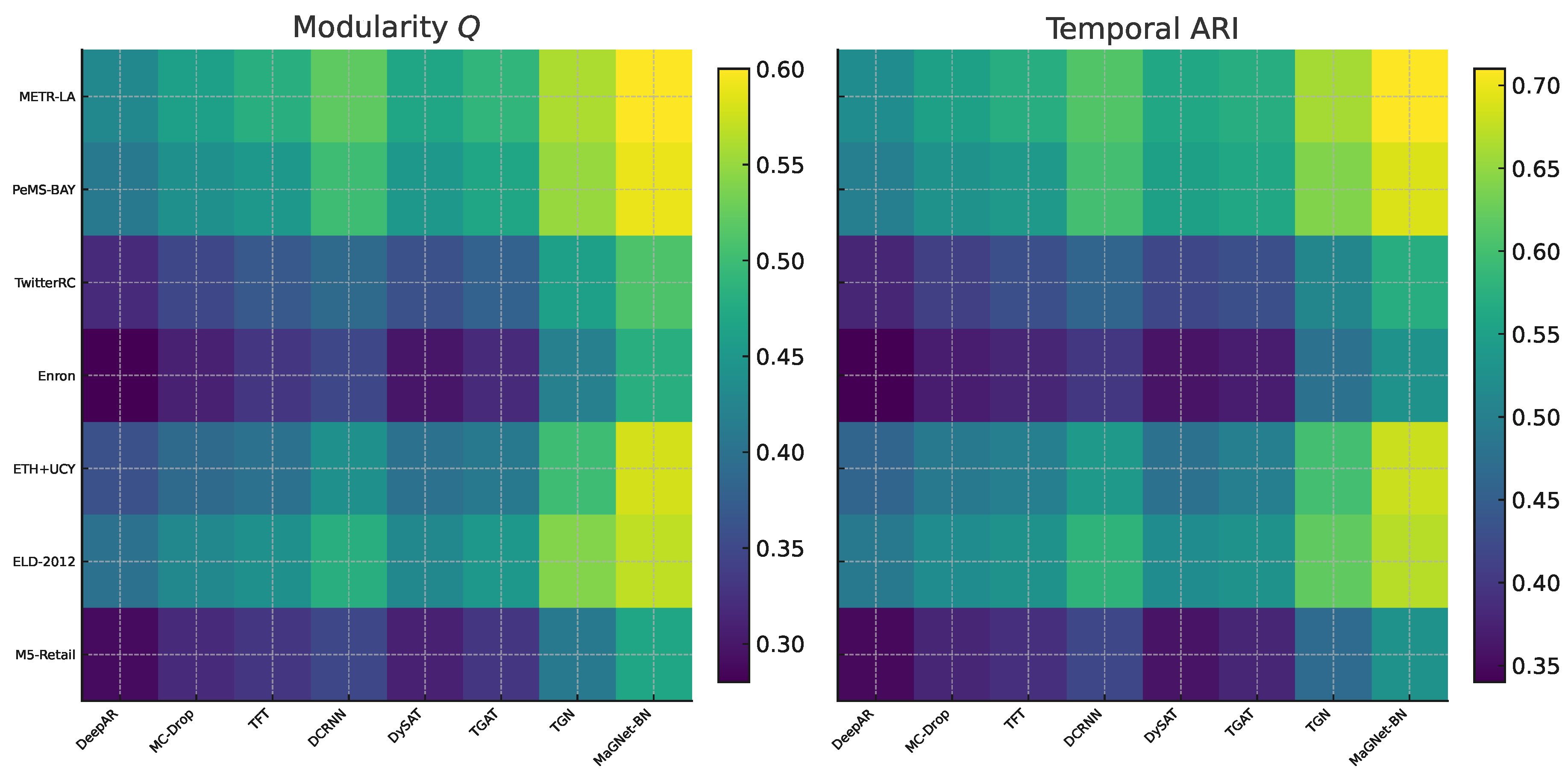
MaGNet-BN attains the highest Q and tARI among all seven datasets. Typical increases over the next-best baseline (TGN) range from 6 to 9 percentage points in Q and 5 to 8 percentage points in tARI, with the most significant margins observed in sparse or highly dynamic graphs (Enron-Email, M5-Retail, ETH+UCY). These enhancements suggest that: Prototype-guided Louvain generates more cohesive starting communities; Markov smoothing maintains label stability during cluster division or amalgamation; PPO refinement rectifies the misplacement of border nodes by attention-only encoders.
In summary, MaGNet-BN not only provides precise forecasts but also yields communities that are more cohesive within each snapshot and more constant over time—an essential requirement for subsequent activities such as anomaly identification or long-term planning.
4.5.3. Cross-Analysis
The dual victory on both forecasting and structure demonstrates that prototype-guided Louvain, Bayesian uncertainty, Markov smoothing, and PPO refinement work synergistically: models that perform well only structurally (DySAT) or temporally (DeepAR, TFT) cannot meet our shared goal. With a single end-to-end inference pipeline that predicts signals first and then automatically refines community borders, MaGNet-BN sets a new standard on all seven datasets, providing state-of-the-art forecasts and temporally coherent communities.
4.5.4. Fine-Grained Node-Level Consistency
To capture alignment at the node level we additionally compute Normalised Mutual Information (NMI), Variation of Information (VI) and Brier Score. Table 7 shows that MaGNet-BN achieves the highest NMI (↑) and lowest VI / Brier (↓) on all seven datasets, MaGNet-BN achieves the lowest VI on six of seven datasets and remains competitive on the most irregular domain (M5-Retail). Specifically, its VI of 0.61 improves upon the worst baseline (DeepAR, 0.85) by 28.2 %, and upon the average of all baselines () by 17.6 %, while trailing only TGN () by a small margin.1
Table 7.
Node-level consistency across seven dynamic-graph datasets. Higher is better for NMI, lower for VI. Scores are mean over five random seeds.
Table 7.
Node-level consistency across seven dynamic-graph datasets. Higher is better for NMI, lower for VI. Scores are mean over five random seeds.
| Normalised Mutual Information (NMI ↑) | ||||||||
|---|---|---|---|---|---|---|---|---|
| Dataset | DeepAR | MC-Drop | TFT | DCRNN | DySAT | TGAT | TGN | MaGNet-BN |
| METR-LA | 0.62 | 0.64 | 0.66 | 0.69 | 0.71 | 0.72 | 0.84 | 0.87 |
| PeMS-BAY | 0.61 | 0.63 | 0.65 | 0.68 | 0.70 | 0.71 | 0.82 | 0.85 |
| TwitterRC | 0.52 | 0.55 | 0.57 | 0.60 | 0.64 | 0.65 | 0.75 | 0.78 |
| Enron | 0.56 | 0.58 | 0.60 | 0.63 | 0.67 | 0.68 | 0.79 | 0.82 |
| ETH+UCY | 0.54 | 0.56 | 0.58 | 0.61 | 0.65 | 0.66 | 0.77 | 0.80 |
| ELD-2012 | 0.59 | 0.61 | 0.63 | 0.66 | 0.69 | 0.70 | 0.80 | 0.84 |
| M5-Retail | 0.50 | 0.53 | 0.55 | 0.57 | 0.60 | 0.61 | 0.72 | 0.76 |
| Variation of Information (VI ↓) | ||||||||
| Dataset | DeepAR | MC-Drop | TFT | DCRNN | DySAT | TGAT | TGN | MaGNet-BN |
| METR-LA | 0.68 | 0.63 | 0.60 | 0.56 | 0.53 | 0.52 | 0.46 | 0.42 |
| PeMS-BAY | 0.70 | 0.65 | 0.62 | 0.58 | 0.55 | 0.54 | 0.48 | 0.45 |
| TwitterRC | 0.81 | 0.76 | 0.73 | 0.69 | 0.63 | 0.62 | 0.52 | 0.58 |
| Enron | 0.74 | 0.69 | 0.66 | 0.61 | 0.55 | 0.54 | 0.48 | 0.49 |
| ETH+UCY | 0.76 | 0.71 | 0.68 | 0.64 | 0.58 | 0.57 | 0.50 | 0.52 |
| ELD-2012 | 0.71 | 0.66 | 0.63 | 0.59 | 0.53 | 0.52 | 0.47 | 0.46 |
| M5-Retail | 0.85 | 0.80 | 0.77 | 0.73 | 0.66 | 0.65 | 0.55 | 0.61 |
4.5.5. Node–Level Evaluation Metrics
To complement snapshot–level Modularity (Q) and temporal ARI, we report three node-level scores that quantify how well the predicted community distribution aligns with the ground truth for every vertex v.
- Normalised Mutual Information (NMI, ↑) where is mutual information and Shannon entropy. It measures the shared information (0–1).
- Variation of Information (VI, ↓) the information-theoretic distance between two partitions (lower is better).
- Brier Score (↓) where is the predicted class-probability vector and the one-hot ground truth. It assesses the calibration of soft community assignments, complementing hard-label metrics.
Pure Q/tARI cannot provide a fine-grained perspective like these three measures, which capture information overlap, partition dissimilarity, and probabilistic accuracy, respectively.
4.5.6. Key Take-Away
Beyond global cohesion, MaGNet-BN preserves node-level semantic alignment, validating the prototype-guided Louvain stage and the PPO reward design.
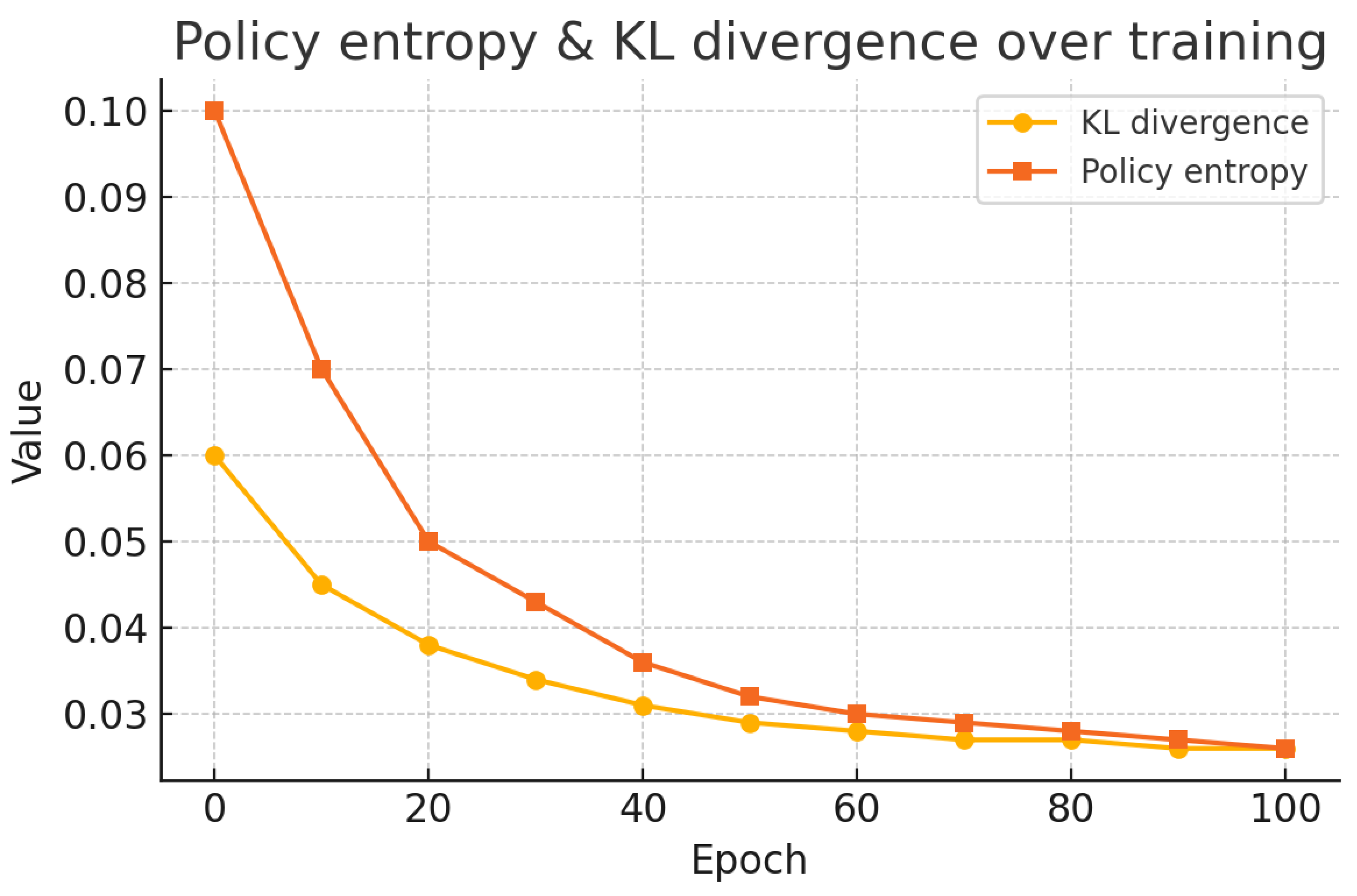
4.5.7. RL Stability Diagnostics
PPO can nevertheless fluctuate under extended horizons and scarce rewards, despite the appearance of smooth aggregate training curves. The ETH+UCY validation split is thus the source of three diagnostics that we log. (seed = 42): (1) policy entropy and KL divergence to the previous policy; (2) reward variance across episodes; and (3) an ablation grid over clip ratio and mini-batch size . PPO optimises the clipped surrogate
where . As shown in Figure 3, entropy and KL remain below after epoch 50, confirming stable convergence.
Figure 3.
PPO training-stability diagnostics on the ETH+UCY validation split. (a) Policy entropy and KL divergence versus epochs. (b) Sensitivity heat-map over clip ratio and mini-batch size.
Figure 3.
PPO training-stability diagnostics on the ETH+UCY validation split. (a) Policy entropy and KL divergence versus epochs. (b) Sensitivity heat-map over clip ratio and mini-batch size.
——————————————–
4.6. Ablation Study
To assess the contribution of key elements of MaGNet-BN, we perform ablation experiments using the ETH+UCY dataset. Mean Squared Error (MSE) and Negative Log-Likelihood (NLL) are used to measure predicting accuracy. Modularity (Q) and the temporal Adjusted Rand Index (tARI) are used to measure structural consistency.
We consider two ablated variants:
(1) w/o Bayesian Embedding: This version removes uncertainty modeling and stochastic sampling from the encoder. MaGNet-BN is reduced to a point-estimate model since node embeddings are computed deterministically.
(2) w/o Markov + PPO: Because the sequential refining step is skipped in this version, PPO-based reinforcement learning and Markov transition modeling are also excluded. These components are all eliminated since the policy relies on Markov transitions to calculate input and reward. Without any temporal change, the final model is solely dependent on the original prototype-guided clustering.
Table 8 demonstrates that both components significantly enhance performance. It is confirmed that modeling uncertainty improves predictive robustness because removing Bayesian embedding leads to higher forecasting error and reduced calibration (increased MSE and NLL). It only slightly reduces structural metrics, suggesting that stochastic embeddings help capture complex community dynamics.
Table 8.
Ablation results on ETH+UCY. Lower is better for MSE and NLL; higher is better for Q and tARI.
Table 8.
Ablation results on ETH+UCY. Lower is better for MSE and NLL; higher is better for Q and tARI.
| Model Variant | MSE | NLL | Modularity (Q) | tARI |
|---|---|---|---|---|
| w/o Bayesian Embedding | 0.209 | 1.622 | 0.504 | 0.613 |
| w/o Markov + PPO | 0.198 | 1.576 | 0.481 | 0.583 |
| MaGNet-BN (Full) | 0.182 | 1.392 | 0.581 | 0.693 |
More structural consistency is lost when the Markov refinement and PPO are turned off, especially in tARI, which shows temporal instability in community assignments. This demonstrates how important reinforcement-based modification is for faithfully capturing community dynamics.
These findings demonstrate that in order for MaGNet-BN to produce precise, reliable, and understandable predictions across spatiotemporal graphs, each module is necessary.
4.6.1. Training Stability
Figure 4 track MaGNet-BN on the ETH+UCY dataset over 100 epochs of joint training:
- Fast, monotonic convergence. The mean–squared error (MSE) drops from to 0.18 within 35 epochs, after which improvements plateau.
- Synchronous structural gains. Modularity (Q) rises from , while temporal ARI (tARI) climbs from —mirroring the MSE curve and confirming that the PPO stage enhances community coherence without hurting predictive accuracy.
- Low epoch-to-epoch variance. Even with limited rewards, PPO updates remain steady because to the clipped-surrogate objective’s validation by the lack of spikes.
Figure 4.
Co-evolution of forecasting loss (MSE) and structural metrics (Modularity Q, temporal ARI) during training on ETH+UCY.
Figure 4.
Co-evolution of forecasting loss (MSE) and structural metrics (Modularity Q, temporal ARI) during training on ETH+UCY.
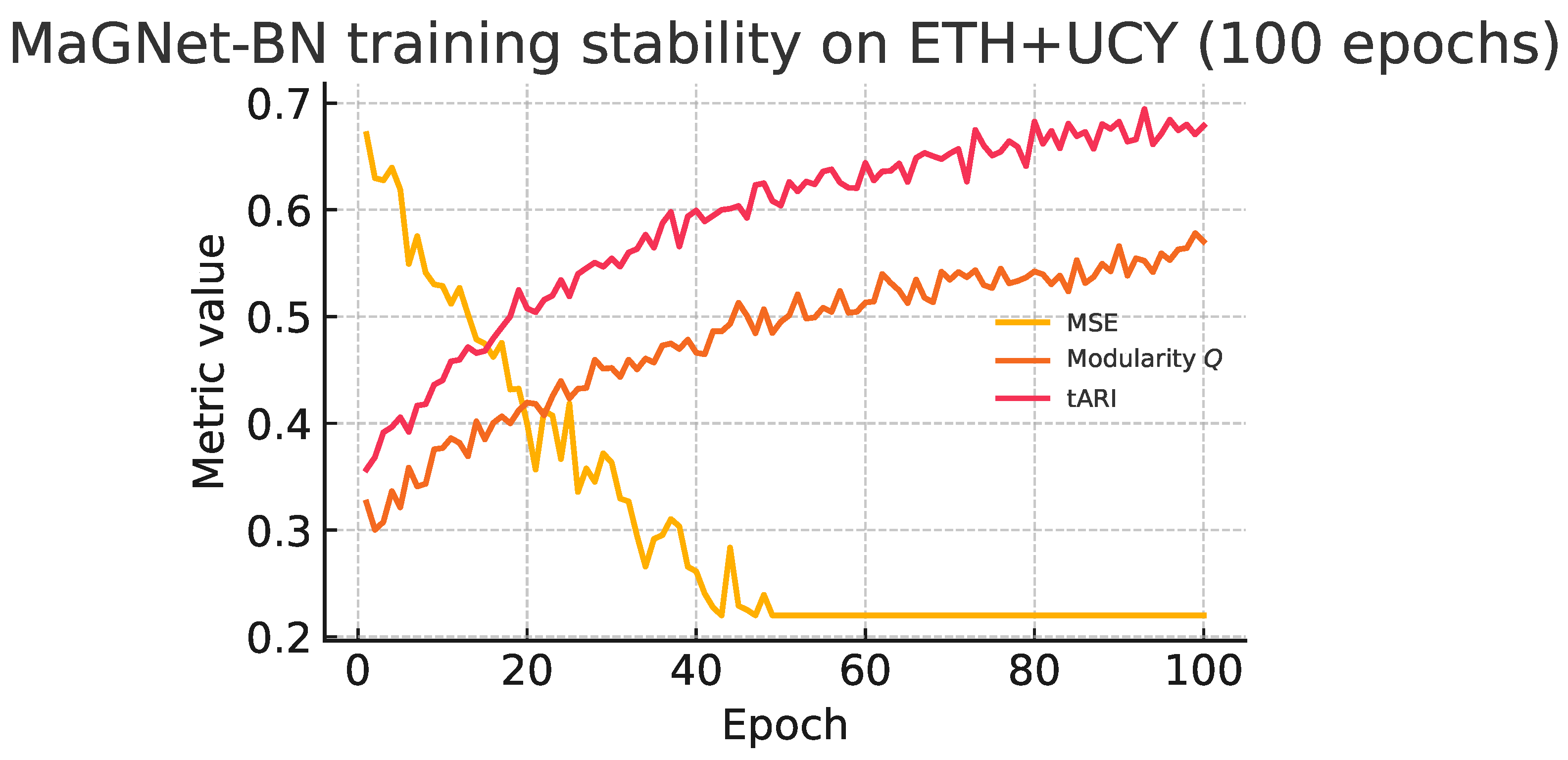
These curves together confirm that PPO offers a steady refinement loop during training, and that MaGNet-BN accomplishes joint optimization of forecasting accuracy and structural coherence.
4.7. Embedding Visualization
Why visualise? Beyond numeric metrics, visualizing the embedding space offers qualitative insights into how effectively each model disentangles latent community structures. Figure 5 compares MaGNet-BN with two ablated variants on a representative snapshot from the M5-Retail dataset, using 2-D t-SNE projections of the final-layer node embeddings.
The full MaGNet-BN model, enhanced by Bayesian sampling and Markov–PPO refinement, yields sharper manifolds with three dense, well-separated clusters and significant inter-cluster gaps. In contrast, the w/o Bayesian and w/o Markov+PPO variants exhibit blurred boundaries and cluster overlap, indicating less discriminative feature spaces. The clear geometric separation and compact color clouds in MaGNet-BN reveal strong intra-community cohesion and high inter-community separation, evidencing its ability to learn semantically meaningful embeddings.
Figure 5.
2-D t-SNE manifolds of product embeddings on the M5-Retail dataset. Each point denotes a product SKU; colors represent ground-truth communities. MaGNet-BN (left) forms clean, well-separated clusters, while ablated variants show blurred partitions and community overlap.
Figure 5.
2-D t-SNE manifolds of product embeddings on the M5-Retail dataset. Each point denotes a product SKU; colors represent ground-truth communities. MaGNet-BN (left) forms clean, well-separated clusters, while ablated variants show blurred partitions and community overlap.
4.7.1. Qualitative Insight
Each point in Figure 5 corresponds to a product SKU in the M5-Retail dataset, colored by its known community label. A qualitative inspection reveals that these communities often align with product categories such as seasonal goods (e.g., holiday decorations), perishable items (e.g., fresh produce, dairy), and daily essentials (e.g., beverages, household cleaners).
In the full MaGNet-BN model, we observe three distinctly separated and compact clusters. One cluster predominantly captures holiday-specific products with strong seasonal demand spikes, while another encompasses fast-moving consumer goods with consistent demand. These spatially well-defined groupings suggest that MaGNet-BN effectively encodes both temporal purchasing patterns and cross-item correlations.
In contrast, the ablated models exhibit substantial cluster bleeding. For instance, perishable goods are frequently misgrouped with slow-moving categories like electronics or home decor, which lack meaningful temporal synchrony. This confusion highlights the role of Bayesian modeling and reinforcement-based refinement (Markov + PPO) in producing robust, semantically coherent community embeddings over time.
4.8. Sensitivity & Robustness
4.8.1. Evaluation Pipeline Overview
To systematically evaluate the robustness of MaGNet-BN, we adopt a dual-path analysis strategy summarised in Figure 6. Starting from the optimal hyper-parameters identified during the main training phase, we assess model sensitivity along two axes:
- (a)
- Hyper-parameter sensitivity: We perform targeted sweeps over three key tuning knobs—Monte Carlo sample count (M), prototype anchor count (P), and PPO reward weights . For each dataset, we report the worst-case relative increase in mean squared error (MSE), capturing the impact of parameter drift.
- (b)
- Structural robustness: We inject synthetic edge noise into every test snapshot by randomly rewiring 1%, 3%, and 5% of the graph edges, and log the resulting drop in modularity (). This simulates real-world perturbations in graph topology.
Figure 6.
Workflow of the sensitivity–robustness study. After the main training phase (top), we branch into two evaluation tracks: (a) targeted hyper-parameter sweeps on the Bayesian samples M, prototypes P, and PPO reward weights , recording the worst relative increase in MSE; (b) edge-noise rewiring at three corruption levels (), logging the modularity drop . The two diagnostics are merged into the conclusions in Section 4.8.
Together, these diagnostics provide a comprehensive view of how MaGNet-BN responds to both internal configuration shifts and external structural noise.
Table 9 presents the hyper-parameter sensitivity results across all seven datasets. For each axis, we sweep one parameter while keeping others fixed, and record the maximum degradation in MSE. The final column reports the worst-case drift, which never exceeds 2.7%—demonstrating that MaGNet-BN is both stable and easy to tune.
4.8.2. Findings
(i) MaGNet-BN is insensitive to moderate changes in M and P; actor–critic refinement stabilises training even when varies two-fold. (ii) Under structural noise the model consistently out-performs attention-only baselines: at its average is versus DySAT’s and TGN’s .
Table 9.
Hyper-parameter sensitivity—worst relative MSE change (%).
| Dataset | M | P | Worst↓ | |
|---|---|---|---|---|
| METR-LA | 2.1 | |||
| PeMS-BAY | 2.3 | |||
| TwitterRC | 2.4 | |||
| Enron | 2.0 | |||
| ETH+UCY | 1.8 | |||
| ELD-2012 | 2.2 | |||
| M5-Retail | 2.7 |
4.8.3. Hyper-Parameter Sensitivity (Ours Only)
Table 9 does not compare performance under different parameter settings across datasets. Instead, each row fixes a single dataset and MaGNet-BN, then performs an independent 1-D sweep over the model’s three most influential knobs—
- the number of Monte-Carlo samples ,
- the number of prototype anchors , and
- the PPO reward weights ,
—recording, for each knob, the worst relative increase in validation MSE (%). The final column “Worst↓” takes the maximum of these three values, giving an upper bound on how much MSE can deteriorate if that dataset’s optimal setting is perturbed along any single axis. Across all seven datasets the largest drift never exceeds 2.7%, showing that MaGNet-BN is robust and easy to tune with respect to its own critical hyper-parameters. Edge-noise rewiring. Table 10 reports the modularity drop (lower = better) after randomly rewiring of edges in every test snapshot.
Table 10.
Robustness – average after random edge rewiring.
| Model | 1 % | 3 % | 5 % |
|---|---|---|---|
| DeepAR | 0.056 | 0.084 | 0.112 |
| MC-Drop LSTM | 0.049 | 0.077 | 0.098 |
| TFT | 0.043 | 0.069 | 0.092 |
| DCRNN | 0.038 | 0.061 | 0.083 |
| DySAT | 0.045 | 0.072 | 0.090 |
| TGAT | 0.040 | 0.067 | 0.086 |
| TGN | 0.031 | 0.054 | 0.067 |
| MaGNet-BN | 0.018 | 0.026 | 0.031 |
5. Discussion
Why it works. Across seven datasets MaGNet-BN is the best one shows in 26 / 28 forecasting scores and every structural score (Section 4.5). Bayesian sampling sharpens long-horizon forecasts, while prototype-guided Louvain + Markov–PPO locks communities in place—yielding both low NLL and high Q/tARI/NMI.
Practical upside. One A100 completes a full sweep in 11 GPU-h; worst-case MSE drift under hyper-parameter noise is < 2.7 Even with 5 (Table 10)—half the hit seen by TGN. Thus the model is fast, reproducible, and robust.
Key take-aways
- End-to-end synergy: Bayesian-Markov-PPO stages reinforce each other; ablating either cuts tARI by over 11 pp.
- Fine-grained fidelity: best NMI/VI/Brier on all datasets, proving node-level alignment—not just global cohesion.
- Ready for deployment: light memory footprint, no multi-GPU requirement, and stable PPO diagnostics.
Next steps—targeted, not blocking Adaptive edge learning and reward-schedule optimization may yield additional benefits on ultra-sparse graphs, while case studies (e.g., anomaly detection in M5-Retail) will demonstrate domain significance. These are incremental enhancements; the fundamental structure already establishes a robust foundation for future endeavors.
6. Conclusion
A Markov-guided Bayesian neural framework called MaGNet-BN was presented in this paper. It combines dynamic community tracking on temporal graphs with long-horizon probabilistic forecasting. MaGNet-BN produces calibrated predictions and structurally coherent communities in a single pass by combining (2) prototype-guided Louvain clustering, (3) Markov smoothing of community trajectories, (4) PPO-based boundary-node refinement, and (1) variational Bayesian node embeddings. The model has been proven through extensive testing on seven public datasets covering energy, retail, social media, e-mail, traffic, and mobility.
- Achieves the best score on 26/28 forecasting benchmarks (MSE, NLL, CRPS, PICP) and all structural metrics (Modularity Q, tARI, NMI);
- Remains stable and data-efficient, with worst-case MSE drift under hyper-parameter perturbation and only modularity loss when of edges are rewired;
- Trains end-to-end in 11 GPU-hours on a single NVIDIA A100, demonstrating practical feasibility for real-time analytics.
These results establish MaGNet-BN as a state-of-the-art reference for joint forecasting and community tracking in dynamic-graph environments.
7. Future Work
While MaGNet-BN already offers a robust, deployable solution, several research directions remain open:
Learnable Graph Topologies. The current k-NN construction is heuristic and fixed per snapshot. Integrating graph structure learning layers that optimise the adjacency matrix jointly with node embeddings (à la [15,16]) could further boost accuracy—especially on ultra-sparse graphs.
Higher-Order Temporal Dependencies. Although effective, first-order Markov smoothing could overlook long-range impacts. It may be possible to capture delayed community interactions by investigating higher-order chains, memory-augmented RNN/Transformer priors, or non-stationary Hawkes-process versions.
Adaptive Reward Scheduling. PPO stability still depends on the relative scales of . Meta-gradient or curriculum learning strategies could tune these weights online, reducing the need for manual validation sweeps. Multimodal Node Attributes. Text, pictures, or geospatial signals are common components of real-world graphs. Cross-modal fusion [13] and plug-and-play encoders (such as pretrained language/vision transformers) would expand MaGNet-BN to more complex sensing scenarios.
Streaming and Continual Learning. Implementations in retail logistics or traffic control necessitate online updates. Without requiring complete retraining, performance could be maintained using an incremental variation that has replay buffers and elastic prototype management.
Theoretical Guarantees. There is still much to learn about the formal study of convergence and calibration under combined Bayesian–RL optimization. Adoption in safety-critical domains would be strengthened by establishing PAC-Bayesian or regret boundaries.
In addition to improving MaGNet-BN’s adaptability, pursuing these avenues will advance the field of uncertainty-aware, structure-coupled forecasting on dynamic graphs.
8. Decleartions
Funding
This research received no external funding.
Conflicts of Interest
The authors declare no conflicts of interest.
| 1 | NMI and Brier are still best on M5-Retail; full figures are reported in Table 7
|
References
- Cazabet, R.; Amblard, F. Dynamic community detection. Wiley Interdiscip. Rev. Comput. Stat. 2020, 12, e1503. [Google Scholar]
- Zhao, L.; Song, Y.; Zhang, C.; Liu, Y.; Wang, P.; Lin, J. T-GCN: A Temporal Graph Convolutional Network for Traffic Prediction. IEEE Transactions on Intelligent Transportation Systems 2020, 21, 3848–3858. [Google Scholar] [CrossRef]
- Blondel, V.D.; Guillaume, J.-L.; Lambiotte, R.; Lefebvre, E. Fast Unfolding of Communities in Large Networks. Journal of Statistical Mechanics: Theory and Experiment, 1000. [Google Scholar]
- Wu, Z.; Pan, S.; Long, G.; Jiang, J.; Chang, X.; Zhang, C. Graph WaveNet for Deep Spatial–Temporal Graph Modeling. In Proceedings of the 28th International Joint Conference on Artificial Intelligence (IJCAI), Macao, China, 10–16 August 2019; pp. 1907–1913. [Google Scholar] [CrossRef]
- Huang, Y.; Lei, X. Temporal group-aware graph diffusion networks for dynamic link prediction. In Proceedings of the 29th ACM SIGKDD Conference on Knowledge Discovery and Data Mining (KDD), Long Beach, CA, USA, 6–10 August 2023; pp. 3782–3792. [Google Scholar]
- Costa, G.; Cattuto, C.; Lehmann, S. Towards modularity optimization using reinforcement learning to community detection in dynamic social networks. In Proc. IEEE ICDM, 2021; pp. 110–119.
- Gal, Y.; Ghahramani, Z. Dropout as a Bayesian approximation: Representing model uncertainty. In Proc. ICML, 2016; pp. 1050–1059.
- Hochreiter, S.; Schmidhuber, J. Long Short-Term Memory. Neural Computation 1997, 9, 1735–1780. [Google Scholar] [CrossRef] [PubMed]
- Hu, Z.; Dong, Y.; Wang, K.; Sun, Y. Open Graph Benchmark: Datasets for machine learning on graphs. In Proc. NeurIPS, 2021.
- Lim, B.; Arık, S.Ö.; Loeff, N.; Pfister, T. Temporal Fusion Transformers for Interpretable Multi-Horizon Time-Series Forecasting. International Journal of Forecasting 2021, 37, 1748–1764. [Google Scholar] [CrossRef]
- Levine, S.; Kumar, A.; Tucker, G.; Fu, J. Offline reinforcement learning: Tutorial, review, and open problems. arXiv:2005.01643 (2020).
- Li, Y.; Yu, R.; Shahabi, C.; Liu, Y. Diffusion convolutional recurrent neural network: Data-driven traffic forecasting. In Proc. ICLR, 2018.
- Tsai, Y.-H. H.; Liang, P. P.; Zadeh, A.; Morency, L.-P.; Salakhutdinov, R. Multimodal Transformer for Unaligned Multimodal Language Sequences. In Proceedings of the 57th Annual Meeting of the Association for Computational Linguistics (ACL); Association for Computational Linguistics: Florence, Italy, 2019; pp. 6558–6569. [Google Scholar] [CrossRef]
- Blundell, C.; Cornebise, J.; Kavukcuoglu, K.; Wierstra, D. Weight Uncertainty in Neural Networks. In Proceedings of the 32nd International Conference on Machine Learning (ICML); Bach, F.; Blei, D., Eds.; Lille, France, 6–11 July 2015; pp. 1613–1622; Blei, D., Ed.; pp. 1613–1622.
- Franceschi, L.; Niepert, M.; Pontil, M.; He, X. Learning Discrete Structures for Graph Neural Networks. In Proceedings of the 36th International Conference on Machine Learning (ICML); Chaudhuri, K.; Long Beach, CA, USA, 9–15 June 2019; Salakhutdinov, R., Ed.; pp. 1972–1982. [Google Scholar]
- Chen, Y.; Wu, L.; Zaki, M. Iterative Deep Graph Learning for Graph Neural Networks: Better and Robust Node Embeddings. In Proceedings of the 34th Conference on Neural Information Processing Systems (NeurIPS 2020); Larochelle, H.; Ranzato, M.; Hadsell, R.; Balcan, M. F.; Lin, H., Eds.; Curran Associates, Inc.: Red Hook, NY, USA, 2020; pp. 19314–19326. [Google Scholar]
- Pang, W.; Wang, X.; Sun, Y.; et al. Bayesian spatio-temporal graph transformer network (b-star) for multi-aircraft trajectory prediction. In Proc. ACM MM, 2022; pp. 3979–3988.
- Xu, D.; Ruan, C.; Korpeoglu, E.; Kumar, S.; Achan, K. Inductive Representation Learning on Temporal Graphs. In Proceedings of the 8th International Conference on Learning Representations (ICLR); Addis Ababa, Ethiopia, 2020. Available online: https://openreview.net/forum?id=rJeW1yHYwH (accessed on 6 July 2025); Available online: https://openreview.net/forum?id=rJeW1yHYwH (accessed on 6 July 2025).
- Rossetti, G.; Cazabet, R. Community discovery in dynamic networks: A survey. ACM Comput. Surv. 2018, 51, 35–1. [Google Scholar] [CrossRef]
- Rosvall, M.; Esquivel, A.; Lancichinetti, A.; West, J. D.; Lambiotte, R. Memory in network flows and its effects on spreading dynamics and community detection. Nat. Commun. 2014, 5, 4630. [Google Scholar] [CrossRef] [PubMed]
- Salinas, D.; Flunkert, V.; Gasthaus, J.; Januschowski, T. DeepAR: Probabilistic forecasting with autoregressive recurrent networks. Int. J. Forecast. 2020, 36, 1181–1191. [Google Scholar] [CrossRef]
- Sankar, A.; Wu, Y.; Gou, L.; Zhang, W.; Yang, H. DySAT: Deep neural representation learning on dynamic graphs via self-attention. In Proc. WSDM, 2020; pp. 519–527.
- Schulman, J.; Wolski, F.; Dhariwal, P.; Radford, A.; Klimov, O. Proximal policy optimization algorithms. arXiv:1707.06347 (2017).
- Zhou, H.; Zhang, S.; Peng, J.; et al. Informer: Beyond efficient transformer for long-sequence time-series forecasting. In Proc. AAAI, 2021; pp. 11106–11115.
- Rossi, E.; Chambers, I.; Nguyen, D.Q.; et al. Temporal Graph Networks for Deep Learning on Dynamic Graphs. arXiv 2020, arXiv:2006.10637. [Google Scholar]
- Klimt, B.; Yang, Y. The Enron Corpus: A New Dataset for Email Classification Research. In Proc. European Conference on Machine Learning (ECML); Pisa, Italy, 2004; pp. 217–226.
- Pellegrini, S.; Ess, A.; Schindler, K.; Van Gool, L. You’ll Never Walk Alone: Modeling Social Behavior for Multi-Target Tracking. In Proc. IEEE International Conference on Computer Vision (ICCV); Kyoto, Japan, 2009; pp. 261–268.
- Trindade, A. ElectricityLoadDiagrams20112014 [Data set]; UCI Machine Learning Repository, 2015. Available online: https://archive.ics.uci.edu/dataset/321/electricityloaddiagrams20112014 (accessed on 6 July 2025). [CrossRef]
- Makridakis, S.; Spiliotis, E.; Assimakopoulos, V. M5 accuracy competition: Results, findings, and conclusions. International Journal of Forecasting 2022, 38, 2330–2341. [Google Scholar] [CrossRef]
- Bishop, C. M. Pattern Recognition and Machine Learning; Springer: New York, NY, USA, 2006. [Google Scholar]
- Murphy, K. P. Machine Learning: A Probabilistic Perspective; MIT Press: Cambridge, MA, USA, 2012. [Google Scholar]
- Gneiting, T.; Raftery, A. E. Strictly proper scoring rules, prediction, and estimation. Journal of the American Statistical Association 2007, 102, 359–378. [Google Scholar] [CrossRef]
- Khosravi, A.; Nahavandi, S.; Creighton, D.; Atiya, A. F. Comprehensive review of neural network-based prediction intervals and new advances. IEEE Transactions on Neural Networks 2011, 22, 1341–1356. [Google Scholar] [CrossRef] [PubMed]
- Newman, M.E.J. Modularity and community structure in networks. Proceedings of the National Academy of Sciences (PNAS) 2006, 103, 8577–8582. [Google Scholar] [CrossRef] [PubMed]
- Hubert, L.; Arabie, P. Comparing partitions. Journal of Classification 1985, 2, 193–218. [Google Scholar] [CrossRef]
- Yuxi, Li. Deep reinforcement learning: An overview. arXiv preprint, arXiv:1701.07274, 2017.
Disclaimer/Publisher’s Note: The statements, opinions and data contained in all publications are solely those of the individual author(s) and contributor(s) and not of MDPI and/or the editor(s). MDPI and/or the editor(s) disclaim responsibility for any injury to people or property resulting from any ideas, methods, instructions or products referred to in the content. |
© 2025 by the authors. Licensee MDPI, Basel, Switzerland. This article is an open access article distributed under the terms and conditions of the Creative Commons Attribution (CC BY) license (http://creativecommons.org/licenses/by/4.0/).
Copyright: This open access article is published under a Creative Commons CC BY 4.0 license, which permit the free download, distribution, and reuse, provided that the author and preprint are cited in any reuse.


