
Submitted:
19 November 2024
Posted:
20 November 2024
You are already at the latest version
Abstract
In recent years, significant advancements have been made in spatiotemporal sequence prediction, with PredRNN++ emerging as a powerful model due to its superior ability to capture complex temporal dependencies. However, the current unidirectional nature of PredRNN++ limits its ability to fully exploit the temporal information inherent in many real-world sequences. In this research, we propose an enhancement to the PredRNN++ model by incorporating a bi-directional network, enabling the model to consider both past and future context during prediction. This bi-directional extension aims to improve the predictive accuracy and robustness of the model, particularly in tasks involving complex temporal dynamics. Our experimental results demonstrate that the bi-directional PredRNN++ outperforms the original model across several benchmark datasets, highlighting its potential for a wide range of applications in spatiotemporal data analysis.
Keywords:
Spatiotemporal data
; Predictive Learning
; Extreme Scale Data Prediction
1. Introduction
Spatiotemporal data integrates spatial information with temporal progression and forms multidimensional datasets [1,2,3,4]. The interpretation of spatiotemporal data necessitates the efficient utilization of spatial data, which is inherently more intricate and diverse than traditional data while incorporating both spatial and temporal aspects. To effectively analyze and interpret the complexities of spatiotemporal data, predictive analytics [5] is employed to forecast future events by analyzing current and historical data, thereby assisting users in identifying upcoming trends, behaviors, and outcomes [6,7]. In the context of spatiotemporal sequence prediction, which has emerged as a critical challenge in various domains from weather forecasting to video understanding, let be a sequence of spatiotemporal data of length T, where represents a spatial state at current time step t () with height , width , and channels. Given the prediction horizon , the goal is to estimate future frames based on the observed sequence [8].
Traditional approaches to this problem have evolved through several key developments in deep learning architectures. Recurrent Neural Networks (RNNs) [9] initially showed promise in handling sequential data, but struggled with preserving long-term dependencies due to the vanishing gradient problem. This fundamental limitation occurs during backpropagation through time, where the gradient signal is repeatedly multiplied by weights and activation derivatives less than 1. This repeated multiplication leads to an exponential decay. As a result, the network fails to effectively learn from early timesteps that may contain critical information for future predictions, as the gradient becomes too weak to meaningfully update the corresponding weights [10].
Long Short-Term Memory (LSTM) networks [11] addressed this limitation through their gating mechanisms, enabling better preservation of temporal information. Further advancement came with Spatiotemporal LSTM (ST-LSTM) [12], which introduced dedicated memory cells for capturing both spatial and temporal features simultaneously. However, these architectures still face significant challenges in modeling complex spatiotemporal dependencies. While they successfully preserve high-level features, they often struggle to maintain fine-grained spatial details over long sequences [4]. Additionally, their unidirectional processing nature limits their ability to capture comprehensive temporal context, as they only consider past information when making predictions.
The introduction of PredRNN [13] marked a significant advancement in addressing these limitations. This architecture implements a dual memory mechanism: local memory cells for preserving detailed spatial information, and a global memory flow for capturing high-level temporal dynamics. PredRNN++ [14] further enhanced this approach by introducing gradient highway units to facilitate better gradient flow during training. PredRNN-v2 [15] added memory decoupling and reverse scheduled sampling, improving the model’s ability to learn from longer temporal contexts.
Despite these improvements, PredRNN-based models still exhibit limitations in long-term prediction tasks due to their inherent unidirectional temporal processing. They process information solely from past to future, potentially missing important temporal dependencies that could be captured by considering future context. Recent research in sequence modeling has shown that bi-directional processing [16] can significantly enhance model performance by enabling information flow in both temporal directions.
Building upon these insights, we propose Bi-PredRNN, an enhanced architecture that extends the PredRNN framework with bi-directional processing capabilities. Our model has two key contributions:
- A bi-directional memory mechanism that processes temporal information in both forward and backward directions, enabling more comprehensive temporal context modeling
- A dynamic window size adaptation mechanism that automatically adjusts the temporal receptive field based on motion complexity in the input sequence
Through extensive experiments on multiple datasets, including Moving MNIST, KTH Action, and climate data, we demonstrate that Bi-PredRNN achieves superior prediction accuracy compared to existing approaches. The rest of this paper details our methodology, experimental validation, and analysis of results. Section 2 reviews related work in spatiotemporal sequence prediction, Section 3 describes our proposed architecture, Section 4 presents the experimental setup and results, and Section 5 concludes with discussions and future directions.
2. Related Works
2.1. Overview of Spatiotemporal Sequence Prediction
Spatiotemporal sequence prediction involves predicting future data points by analyzing both spatial and temporal dependencies in a sequence of data. This type of prediction is crucial for applications such as video processing, weather forecasting, and traffic flow prediction. Challenges arise from the need to capture two aspects: spatial correlations that represent relationships between different locations, and temporal dynamics that describe the evolution of these relationships. The spatial aspect of prediction involves understanding relationships between different locations or features in a given space. Yu et al. [17] formalized this as a graph structure where nodes represent spatial locations and edges capture their interactions in their seminal work on traffic forecasting. This graph-based framework has become fundamental in modern approaches to spatiotemporal modeling. For grid-structured data, Shi et al. [4] introduced the ConvLSTM architecture that effectively captures spatiotemporal correlations in regular grids, establishing a foundation for applications like precipitation forecasting. Temporal dependencies capture how patterns evolve over time, often exhibiting both short-term and long-term characteristics, requiring models to capture multiple temporal scales simultaneously.
2.2. Spatiotemporal Convolutional Neural Networks
Spatiotemporal Convolutional Neural Networks (CNN) extend traditional 2D CNNs to capture temporal dynamics in video data. Early architectures focused on direct 3D convolutions for video understanding tasks [18,19], particularly in action recognition and temporal feature extraction [20]. These architectures have evolved into more complex designs that break down spatiotemporal features using factorized convolutions [21,22]. Notably, the probabilistic perspective introduces frameworks where temporal and spatial features are processed through separate 2D and 1D convolutional pathways [23], enhancing both computational efficiency and interpretability of learned representations.
Convolutional LSTM (ConvLSTM) architectures represent a significant advancement, fundamentally redesigning the LSTM cell structure to accommodate convolutional operations [4]. The authors combined graph convolutional layers composed of spatiotemporal convolutional blocks with a convolutional sequence learning layer, utilizing convolutional structure along the time axis to fully leverage spatial information. Recent advances have also focused on memory-efficient implementations and real-time processing capabilities, introducing innovations in sparse convolution techniques [24] and adaptive temporal sampling strategies [25].
2.3. Spatiotemporal Long Short-Term Memory
Long Short-Term Memory (LSTM) networks have evolved beyond their original sequence modeling capabilities to address the complex challenges of spatiotemporal prediction [11]. The integration of spatial features with LSTM’s temporal modeling has led to several innovative architectures specifically designed for spatiotemporal forecasting tasks. ST-LSTM [12] represents a fundamental architecture in this evolution, designed to process both spatial and temporal features simultaneously. By incorporating dedicated processing paths for spatial and temporal information streams, ST-LSTM effectively captured spatiotemporal dependencies for sequence prediction tasks. Several architectures have emerged combining the advantages of both ST-LSTM and ConvLSTM approaches. The Memory In Memory (MIM) network [26] introduced a more sophisticated memory mechanism that can learn higher-order non-stationary transitions in spatiotemporal data, making it particularly effective for complex prediction tasks involving multiple temporal frequencies.
As shown in Figure 1, i represents the input gate, f is the forget gate, c is the cell state, g is the candidate cell state, o is the output gate, and h is the hidden state. In Conv LSTM, the spatiotemporal memory state serves as its feature, while in PredRNN, M represents the spatial memory and C denotes the temporal memory.
2.4. Multi Modal Prediction & Attention Models
The landscape of spatiotemporal prediction has evolved significantly beyond traditional recurrent architectures, incorporating more sophisticated approaches to handle the increasing complexity of real-world data. While RNN-based models process information sequentially, modern architectures leverage attention mechanisms that enable direct modeling of relationships between any elements in the input sequence, regardless of their temporal distance. This shift has been particularly important in handling multi-modal data, where information from different sources must be integrated coherently. Additionally, the emergence of graph-based approaches has provided a natural framework for modeling complex spatial interactions, while transformer architectures have demonstrated remarkable capability in capturing long-range dependencies through their self-attention mechanisms. These architectural innovations have been crucial in addressing key challenges in spatiotemporal prediction, including the need to handle missing data, integrate multiple data modalities, and model complex interaction patterns.
Recent advancements in spatiotemporal prediction have seen promising results in incorporating multi-modal data and handling complex interaction patterns. Junan Chen et al. [27] proposed a spatiotemporal graph neural network that explicitly models vehicle interactions for trajectory prediction. Their approach combines attention mechanisms with graph neural networks to capture both spatial relationships and temporal dependencies between vehicles in complex traffic scenarios. The integration of self-supervised learning techniques has also shown promise in improving spatiotemporal forecasting. Weyn et al. [28] introduced a novel multi-modality framework that leverages self-supervised learning to capture correlations across different data modalities. Their approach addresses the challenge of learning from multiple data sources while maintaining computational efficiency, particularly valuable for applications involving diverse sensor inputs. Furthermore, environmental monitoring applications have driven innovations in handling missing data in spatiotemporal sequences. Kumar et al. [29] developed SERT, a transformer-based architecture specifically designed for environmental sensor data with missing values. Their model combines spatial and temporal attention mechanisms with specialized embedding techniques to handle irregular sampling and missing observations, demonstrating robust performance in real-world environmental monitoring scenarios.
2.5. Limitations of Current Approaches
Recent advances in spatiotemporal prediction models have demonstrated significant progress in capturing complex temporal dependencies and spatial relationships. However, several fundamental limitations persist in current approaches and reduce their effectiveness in real-world applications. This section analyzes these limitations and presents our research position addressing these challenges.
A primary challenge in RNN-based architectures is the persistent issue of vanishing gradients during backpropagation through time (BPTT) [30]. While various techniques such as gradient clipping and careful initialization have been proposed [31], these solutions provide only partial remedies and often fail in scenarios requiring long-term dependency modeling [10]. This limitation becomes particularly apparent in applications requiring extensive temporal context, such as long-term weather forecasting or traffic prediction.
The integration of spatial and temporal features presents another significant challenge. Traditional Fully Connected LSTM architectures, by treating spatial information as flat vectors, inherently lose crucial spatial relationships that are essential for accurate prediction [4]. Although ConvLSTM architectures have attempted to address this by introducing spatial operations, they still struggle with maintaining long-range spatial dependencies effectively [20]. The fundamental trade-off between preserving spatial features and maintaining temporal memory remains suboptimal, particularly in scenarios involving complex spatial transformations [14].
Data efficiency and scalability concerns significantly impact the practical deployment of current models. Transformer-based approaches, despite their powerful representation capabilities, exhibit considerable data hunger due to their limited inductive biases [32]. The quadratic scaling of self-attention mechanisms with sequence length imposes practical challenges on their application to long sequences [33]. Furthermore, the extensive pre-training requirements make these models particularly resource-intensive for specialized domains. This makes them inaccessible to researchers with limited computational resources [34].
Model adaptability represents another critical limitation. Current approaches, such as 3D CNN with DropPath (also known as Drop Connect, is a regularization technique used in deep neural networks where randomly selected paths or connections between layers are temporarily set to zero during training.), typically require complete retraining for new datasets [35] This lack of transfer learning capabilities not only increases computational overhead but also limits the models’ practical utility in real-world scenarios where data distributions may shift over time [36]. The challenge of domain adaptation becomes particularly acute in specialized architectures, where the model’s performance can degrade significantly when applied to slightly different domains.
3. Method
In this section, we present a comprehensive description of our proposed bi-directional Predictive Recurrent Neural Network (Bi-PredRNN). Our methodology introduces two principal contributions to the field of spatiotemporal prediction. First, we propose a novel bi-directional memory network architecture that systematically integrates both antecedent and subsequent temporal information in the feature representation process. This approach enables more robust modeling of long-term dependencies through detailed temporal context utilization. Second, we demonstrate the model’s versatility across diverse data representations, successfully applying it to both regular grid-structured data (e.g., 2D dynamics) and complex irregular spatiotemporal patterns (e.g., climate datasets). This cross-domain applicability validates the generalization of our approach across varying data representations and temporal scales.
3.1. Bi-Directional Memory
Our model integrates bi-directional LSTM processing into long-term memory learning to overcome the limited temporal context modeling of unidirectional approaches. The introduction of bi-directional processing represents a significant paradigm shift in spatiotemporal prediction for several key reasons [16,37,38]. By solely leveraging past information, traditional unidirectional models create an inherent information bottleneck that limits their predictive capabilities. As illustrated in Figure 2, our bi-directional approach enables more comprehensive context utilization through dual paths of information flow, significantly mitigating the vanishing gradient problem through multiple gradient propagation routes.
The dual memory approach in Bi-PredRNN creates a more robust feature representation mechanism by capturing both forward and backward temporal dependencies simultaneously. The forward path maintains causal relationships essential for prediction, while the backward path incorporates future context that enables more accurate long-term forecasting [13,14]. This comprehensive approach to temporal modeling allows the network to leverage a more complete set of spatiotemporal relationships.
Our model implements several key contributions to enhance its effectiveness. First, the dual memory integration mechanism maintains spatial coherence through specialized memory cells while enabling efficient information flow between the forward and backward paths. Second, the enhanced feature capture mechanism preserves spatial relationships through structured memory organization, ensuring that critical spatial information is not lost during temporal processing. Finally, our adaptive processing framework dynamically adjusts feature importance through learned attention mechanisms, balancing computational efficiency with model expressiveness.
3.2. Theoretical Framework of Bi-Directional Memory Flow
Let be a spatiotemporal sequence, where represents a spatial state at time with height H, width W, and channels C. The bi-directional memory flow operates by maintaining two complementary hidden states: a forward hidden state that processes the sequence from to T, and a backward hidden state that processes from to 1. As illustrated in Figure 2, these bi-directional paths are implemented through cascaded memory cells with convolution operations and layer normalization.
The core principle of this architecture is to integrate both causal and predictive patterns through bi-directional processing. At each time-step t, the complete representation is derived from these bi-directional states:
where denotes the memory update function, and are the learnable parameters for forward and backward processes respectively, and represents the fusion function that integrates the bi-directional information. The memory update function incorporates both spatial and temporal dependencies through a CausalLSTM [14] architecture:
where is the sigmoid function, ⊙ denotes element-wise multiplication, and W and b are learnable parameters.
3.3. Training Strategy and Loss Functions
The training of Bi-PredRNN employs a carefully designed loss function that addresses multiple aspects of spatiotemporal prediction quality. The total loss is composed of three main components:
The first term, reconstruction loss, ensures accurate frame-level predictions by minimizing the mean squared error between predicted and ground truth frames:
where and denote the ground truth and predicted frames at time step t, respectively. This loss directly measures the pixel-wise accuracy of predictions, encouraging the model to generate visually accurate frames.
The second term introduces temporal coherence by penalizing inconsistencies in frame-to-frame transitions:
where represents frame-to-frame differences. This loss ensures smooth temporal transitions by matching the dynamics between consecutive frames in both predicted and ground truth sequences, reducing temporal artifacts such as jittering or sudden changes.
The third term, bi-directional consistency loss, enforces agreement between forward and backward predictions:
where and represent the hidden states from forward and backward passes respectively. This loss term encourages the model to learn consistent representations regardless of sequence direction, leading to more robust predictions.
The weighting coefficients , , and are set to 1.0, 0.5, and 0.2 respectively, based on empirical validation. These weights balance the contribution of each loss component, with higher weight on reconstruction accuracy while maintaining temporal coherence and bi-directional consistency.
3.4. Multi-Layer Implementation
The theoretical framework is implemented through a K-layer architecture where each layer maintains its hidden state and cell state . Although deeper architectures generally enable the capture of more sophisticated features, we adopt the widely-used 4-layer configuration (K=4) that has been empirically validated across various spatiotemporal prediction tasks. As illustrated in Figure 3, the network processes information in both forward and backward directions with cascaded memory flow across time steps.
The network first processes information in the forward direction. For time-step t from 1 to T:
Following the forward pass, the network processes information in the backward direction. For time-step t from T to 1:
The hidden states from forward and backward passes are first concatenated:
The final prediction for the next time step is then generated through a dimensionality reduction layer:
where Conv2D is a 1×1 convolutional layer that reduces the channel dimension to match the input dimension. This multi-layer structure enables sophisticated spatiotemporal pattern modeling through hierarchical feature extraction and bi-directional information flow. Note that in both passes, the spatial memory from the highest layer ( and ) flows to the lowest layer of the next time step ( for forward pass, for backward pass). This cascade memory flow allows the model to maintain long-term spatial dependencies across time steps while processing information bi-directionally.
3.5. Dynamic Window Size Mechanism
We propose a dynamic window size mechanism that adaptively adjusts the temporal processing window based on the motion between frames. This approach aims to balance computational efficiency with prediction accuracy by varying the temporal context according to the observed motion patterns. The window size configuration is governed by three key parameters: minimum window size (), maximum window size (), and EMA smoothing coefficient (). The minimum window size ensures basic temporal dependency modeling while maintaining computational efficiency for low-motion sequences. The maximum window size is empirically determined to capture extended temporal dependencies in high-motion sequences while maintaining reasonable computational costs. The EMA smoothing coefficient prevents rapid oscillations in window size, ensuring temporal consistency in predictions.
3.5.1. Optical Flow Based Motion Estimation
The motion estimation is performed using a lightweight convolutional neural network that consists of three layers:
where represents the concatenated input of two consecutive frames, and denotes a convolutional operation with kernel size k and channel dimensions . The network progressively processes the spatial information while maintaining the ability to capture motion patterns at different scales through its hierarchical structure. The motion magnitude is computed as the average magnitude of optical flow vectors across all spatial locations:
where and represent the horizontal and vertical components of the optical flow at spatial position , respectively, and are the height and width of the feature map.
3.5.2. Adaptive Window Size Selection
The window size is determined through a three-step process:
Base Window Size is:
where is the sigmoid function that maps the motion magnitude to a value between 0 and 1. Temporal Smoothing using Exponential Moving Average (EMA) is
where and represent the smoothed window sizes at the current and previous time steps, respectively. Window Size Parity Adjustment is
The final window size determines the temporal context for both forward and backward passes:
where T is the total number of frames in the sequence.
4. Experiments
We evaluated the performance of our proposed method using the following datasets: Moving MNIST, KTH Action dataset, ToSNA (North Atlantic) SST dataset, and the Global Climate dataset. The first two datasets are widely-used benchmarks for sequence prediction tasks, while the latter two provide real-world climate data to validate our model’s applicability to environmental forecasting problems. All models were implemented using PyTorch framework [39] and trained until convergence using the Adam optimizer. We employed an L2 loss (mean squared error, MSE) function for all experiments and tuned the hyperparameters with the learning rate initialized at .
4.1. Moving MNIST Dataset
For the Moving MNIST dataset [40], we evaluate our model’s predictive performance by generating 10 future frames given 10 input frames. The dataset consists of sequences where digits move and bounce within a 64 × 64 pixel frame. The input data is structured with clips array of shape where 2 represents the number of moving digits, 10000 represents the number of data samples, and 2 represents coordinates of each digit, dims array of shape where 1 is the batch size and 3 represents spatial dimensions, and input_raw_data array of shape where 200000 is the total number of frames, 1 represents the channel number (grayscale), and represents the height and width of the image in pixels. The raw input data has a mean pixel value of 0.047 and a standard deviation of 0.194, indicating a sparse presence of digits in the frames. We split the dataset into 10,000 training sequences and 3,000 validation sequences, with digits in the validation set drawn from different portions of the MNIST dataset than those used in training. Additionally, we assess the model’s generalization capability by testing the models trained on two-digit sequences against sequences containing three moving digits.
4.2. KTH Dataset
For the KTH dataset [41], we evaluate our model’s predictive performance by generating 10 future frames given 10 input frames. The dataset consists of sequences where human subjects perform six types of actions (walking, jogging, running, boxing, handwaving, and handclapping) in four different scenarios (outdoors, outdoors with scale variation, outdoors with different clothes, and indoors). Each sequence is recorded at 25fps and downsampled to pixel frames. The input data is structured with input_raw_data array of shape , where N represents the total number of frames across all sequences, 1 represents the grayscale channel, and represents the height and width of the image in pixels. The raw input data has been preprocessed to normalize pixel values between 0 and 1, with background pixels typically having values close to 0 and foreground (human subjects) showing higher intensity values.
We organize the dataset into training, validation, and test sets following a person-based splitting strategy, where sequences from 16 subjects are used for training, 4 for validation, and 5 for testing. This ensures that the model learns to generalize across different individuals rather than memorizing specific subjects’ movements. Each action sequence is temporally segmented into multiple subsequences of 20 frames (10 for input, 10 for prediction) with a sliding window approach, resulting in approximately 7,000 training sequences. The validation and test sets contain approximately 1,800 and 2,200 sequences respectively. Additionally, we assess the model’s robustness by evaluating its performance across different scenarios, particularly focusing on its ability to handle variations in clothing, scale, and background conditions.
4.3. Climate Dataset
For the climate datasets, we analyze two distinct but related spatiotemporal datasets derived from the Community Earth System Model (CESM2) pre-industrial control experiment: a global surface air temperature dataset and a North Atlantic sea surface temperature (SST) dataset [42]. These datasets enable the evaluation of our model’s capacity to capture complex climate system dynamics under controlled conditions. A sample of projected worldwide map is described in Figure 4.
The global temperature dataset consists of monthly averaged fields spanning 1200 years, with a spatial resolution of 192 × 288 grid points (latitude × longitude), resulting in a data tensor of shape (14389, 192, 288). The input data has been preprocessed to remove the climatological seasonal cycle, focusing on deviations that represent internal climate system variability. The normalized temperature data shows near-zero mean with a standard deviation of 0.708, reflecting the successful removal of systematic seasonal variations. The spatial coordinates are represented by latitude arrays (shape: 192, std: 52.233) and longitude arrays (shape: 288, mean: 179.375, std: 103.922), providing complete global coverage.
The North Atlantic SST dataset (ToSNA) focuses on a specific region with dimensions (14389, 70, 125), representing 800 years of monthly data at a nominal 1° horizontal resolution. The data has been carefully curated to maintain scientific validity, with no missing values (NaN count: 0) and a temperature range from -1.80°C to 30.41°C, with a mean of 11.28°C. To isolate internal climate variability, we employ two key preprocessing steps: (1) removing the time-mean SST at each geographical location to eliminate latitudinal variation, and (2) applying a 12-month moving average at each location to remove the seasonal cycle.
We structure our evaluation framework to assess both spatial and temporal prediction capabilities, with a particular focus on the model’s ability to capture internal climate system dynamics when external forcing is held constant. The dataset split maintains temporal coherence while ensuring sufficient data for both training and validation. Additionally, we evaluate the model’s ability to capture various known climate patterns and oscillations, providing a robust test of its capacity to learn complex Earth system dynamics.
4.4. Evaluation Metrics
We utilize three primary metrics—MSE, PSNR, and SSIM—to evaluate the performance of the models. Each metric provides a unique perspective on assessing the similarity between the predicted and ground truth frames.
MSE (Mean Squared Error) measures the average squared difference between the predicted and ground truth frames. A lower MSE indicates that the predicted frame is closer to the actual frame. MSE is defined as follows:
where represents the pixel value of the ground truth frame, is the pixel value of the predicted frame, and m and n denote the height and width of the frame, respectively.
PSNR (Peak Signal-to-Noise Ratio) is derived from MSE and represents the ratio between the maximum possible power of a signal and the power of noise, in a logarithmic scale. A higher PSNR indicates that the predicted frame has a higher similarity to the ground truth frame. PSNR is defined as:
where is the maximum possible pixel value of the image (e.g., for 8-bit images). PSNR complements MSE by emphasizing the perceptual quality of the image.
SSIM (Structural Similarity Index Measure [43]) measures the structural similarity between the predicted and ground truth frames by considering luminance, contrast, and structural information. SSIM ranges from 0 to 1, where a value closer to 1 indicates higher structural similarity. SSIM is calculated as follows:
where and represent the mean pixel values of the ground truth frame I and the predicted frame , and denote the variances of the ground truth and predicted frames, respectively, indicates the covariance between I and , and and are small constants used to stabilize the division.
SSIM is particularly effective for assessing image structural similarity, often correlating better with human perceptual quality than PSNR or MSE alone. Each of these metrics provides a different lens through which the quality of the predicted frames can be analyzed and helps to comprehensively assess how well the proposed model approximates the ground truth frames.
5. Results
We evaluated our bi-directional approach with dynamic window size adaptation using SSIM and MSE. Table 1 presents a comparative analysis of our model against state-of-the-art approaches. SSIM provides a comprehensive assessment of structural similarity between predicted and ground truth frames, ranging from -1 to 1, with higher scores indicating better prediction quality. Table 1 presents a comparative analysis of our model against state-of-the-art approaches. Notably, we include the baseline PredRNN model (Wang et al., 2018 [13]) to demonstrate the impact of our bi-directional memory flow and dynamic temporal window mechanism.
Our experimental results show that the adaptive window size mechanism, which ranges from to frames, effectively captures both short-term and long-term dependencies in the sequence. The motion-adaptive processing window, governed by our optical flow estimator and EMA smoothing (), allows the model to allocate computational resources more efficiently based on the temporal dynamics of the input sequence. For the 10-frame prediction task, our model achieves comparable performance to existing approaches, particularly in sequences with varying motion intensities. This suggests that our bi-directional architecture can effectively leverage both past and future context through its dynamic window adaptation.
We extended the prediction horizon from 10 to 30 frames to evaluate the temporal prediction limits of our model. While the model maintains competitive performance in terms of SSIM and MSE metrics for longer sequences, we observe that the prediction quality gradually decreases, particularly in regions with high motion complexity where the dynamic window size approaches its upper limit (). This degradation can be attributed to the accumulation of uncertainty in long-term predictions and the inherent limitations of the temporal window size in capturing extended dependencies. Based on these observations, we focus our subsequent analysis on the 10-frame prediction task, where our model demonstrates more stable and reliable performance.
In Figure 5, we present examples of predicted frames that demonstrate the superior performance of our Bi-directional PredRNN model with dynamic window size adaptation. The quantitative results show that our model achieves better performance across all metrics on the Moving MNIST dataset (MSE: 47.60, PSNR: 31.34, SSIM: 0.90) compared to existing approaches, including PredRNN++ (MSE: 50.70, PSNR: 31.08, SSIM: 0.89).
When evaluating on the KTH action dataset, we observe an interesting pattern in our model’s performance. The basic Bi-directional PredRNN shows slightly degraded performance (SSIM: 0.75) compared to PredRNN++ (SSIM: 0.87), which can be attributed to the increased complexity of human motion patterns and the potential over-fitting of the bi-directional architecture to local temporal dependencies. However, with the introduction of our dynamic window size adaptation mechanism, the model significantly improves its performance (MSE: 91.28, PSNR: 29.25, SSIM: 0.88), surpassing PredRNN++ in PSNR metrics and achieving comparable SSIM scores.
This performance improvement can be attributed to the synergistic effect of bi-directional processing and dynamic window size adaptation: while the bi-directional architecture provides comprehensive temporal context understanding, the dynamic window size mechanism prevents over-reliance on either local or global temporal features, resulting in more balanced and accurate predictions.
For the ToSNA dataset, our model shows steady improvement over baseline approaches, with the dynamic window size adaptation mechanism further enhancing prediction accuracy (MSE: 48.25, PSNR: 27.29, SSIM: 0.84) compared to the conventional ConvLSTM (MSE: 60.30, PSNR: 26.32, SSIM: 0.78). Regarding the climate dataset, while our model shows promising results (MSE: 37.25, PSNR: 28.60, SSIM: 0.82) and outperforms existing approaches, it’s important to note some methodological considerations. Unlike traditional validation approaches, the climate dataset was processed sequentially due to its temporal nature, with later time periods serving as test data. This temporal split, while practical for climate data analysis, may introduce potential risks of overfitting since the validation set wasn’t randomly sampled from the entire dataset. The strong temporal correlations inherent in climate data, combined with this sequential validation approach, suggest that the reported performance metrics should be interpreted with some caution. Future work might benefit from exploring alternative validation strategies or incorporating additional regularization techniques specifically designed for temporally correlated data.
This performance improvement across datasets can be attributed to the synergistic effect of bi-directional processing and dynamic window size adaptation: while the bi-directional architecture provides comprehensive temporal context understanding, the dynamic window size mechanism prevents over-reliance on either local or global temporal features, resulting in more balanced and accurate predictions.
5.1. Qualitative Works
In Figure 5, we analyze the qualitative performance of our Bi-directional PredRNN model with dynamic window size adaptation across both Moving MNIST and KTH action datasets. For Moving MNIST sequences, our model maintains sharp digit boundaries and preserves distinctive numerical features (e.g., the curve in ’0’, ’8’) without distortion. The model accurately predicts the trajectory changes when digits collide, and it demonstrates physically plausible reflection patterns at frame boundaries.
The KTH action sequences show our model’s capability to handle complex human motion patterns. The dynamic window size adaptation mechanism is particularly effective for the capture of natural human movements because it automatically adjusts the temporal receptive field based on motion complexity. The results show smooth and continuous predictions of coordinated body movements, from the synchronized motion of arms and legs during walking to precise finger movements in hand-waving actions. Our model consistently maintains temporal coherence and preserves subtle details such as clothing folds and shadow interactions under various lighting conditions.
6. Conclusions
We have tackled key challenges in spatiotemporal sequence prediction, focusing on the difficulties of capturing complex temporal dependencies and preserving spatial coherence in long sequences. Traditional models often struggle with these tasks due to the vanishing gradient problem and limitations in maintaining spatial information over time. Bi-PredRNN extends PredRNN by incorporating bi-directional processing capabilities to address these challenges.
Our primary contribution is a bi-directional memory network architecture that processes temporal information in both forward and backward directions, with specialized memory cells to ensure spatial coherence. We have also introduced a dynamic window size mechanism, which adapts temporal context based on optical flow estimation and EMA smoothing, allowing for more flexible temporal processing. Experimental results on datasets such as Moving MNIST, KTH Action, and climate data demonstrate that our model achieves improved prediction accuracy and more stable long-term dependencies compared to traditional unidirectional models.
Despite these advancements, we recognize limitations in spatiotemporal prediction due to inherent temporal ambiguity. While bi-directional processing enriches temporal context, it can introduce uncertainty when future states significantly influence past interpretations. This motivates the development of advanced temporal attention mechanism that dynamically adjust the weight of past and future contexts. Hybrid architectures, which adapt between unidirectional and bi-directional processing based on the sequence’s temporal features, may also help. Finally, adding domain-specific knowledge could reduce temporal ambiguity in specialized applications.
Author Contributions
Conceptualization, S.-H.H., D.-J.C. and T.-S.C.; methodology, S.-H.H.; software, S.-H.H.; validation, S.-H.H., D.-J.C. and T.-S.C.; formal analysis, S.-H.H., D.-J.C., and T.-S.C.; investigation, S.-H.H. and D.-J.C.; resources, T.-S.C.; data curation, S.-H.H.; writing—original draft preparation, S.-H.H.; writing—review and editing, S.-H.H., D.-J.C. and T.-S.C.; visualization, S.-H.H. and D.-J.C.; supervision, T.-S.C.; project administration, T.-S.C.; funding acquisition, T.-S.C. All authors have read and agreed to the published version of the manuscript.
Funding
This work was supported by Institute of Information & communications Technology Planning & Evaluation (IITP) under the Artificial Intelligence Convergence Innovation Human Resources Development (IITP-2024-RS-2023-00255968) grant and the ITRC (Information Technology Research Center) support program (IITP-2021-0-02051) funded by the Korea government(MSIT).
Informed Consent Statement
Not Applicable.
Data Availability Statement
In this study, we utilized four publicly available datasets: Moving MNIST, KTH Action, and ToSNA&Climate datasets. The Moving MNIST dataset is accessible at https://www.cs.toronto.edu/~nitish/unsupervised_video/ (accessed on 25 October 2024). The KTH Action dataset can be found at https://www.csc.kth.se/cvap/actions/ (accessed on 25 October 2024). For the climate data analysis, we used the spatiotemporal variability of sea surface temperature (SST) in the North Atlantic from the pre-industrial control simulation (piControl) of the Community Earth System Model (CESM2) as part of the sixth phase of the Coupled Model Intercomparison Project (CMIP6). The CESM2 data, which uses the Community Atmosphere Model (CAM6) and Parallel Ocean Program (POP2) at a nominal 1° horizontal resolution, is publicly available from the CMIP archive at https://esgf-node.llnl.gov/projects/cmip6 (accessed on 25 October 2024) and its mirrors.
Conflicts of Interest
The authors declare no conflicts of interest.
References
- Cressie, N.; Wikle, C.K. Statistics for spatio-temporal data; John Wiley & Sons, 2011. [Google Scholar]
- Andrienko, N.; Andrienko, G. Visual analytics of movement: An overview of methods, tools and procedures. Information visualization 2013, 12, 3–24. [Google Scholar] [CrossRef]
- Stein, M.L. Space–time covariance functions. Journal of the American Statistical Association 2005, 100, 310–321. [Google Scholar] [CrossRef]
- Shi, X.; Chen, Z.; Wang, H.; Yeung, D.Y.; Wong, W.K.; Woo, W.c. Convolutional LSTM network: A machine learning approach for precipitation nowcasting. Advances in neural information processing systems 2015, 28. [Google Scholar]
- Mishra, N.; Silakari, S. Predictive analytics: A survey, trends, applications, oppurtunities & challenges. International Journal of Computer Science and Information Technologies 2012, 3, 4434–4438. [Google Scholar]
- Ranjeeth, S.; Latchoumi, T.P.; Paul, P.V. A survey on predictive models of learning analytics. Procedia Computer Science 2020, 167, 37–46, Publisher: Elsevier. [Google Scholar] [CrossRef]
- Eckerson, W.W. Predictive analytics. Extending the Value of Your Data Warehousing Investment. TDWI Best Practices Report 2007, 1, 1–36. [Google Scholar]
- Seo, Y.; Defferrard, M.; Vandergheynst, P.; Bresson, X. Structured Sequence Modeling with Graph Convolutional Recurrent Networks. In Neural Information Processing; Cheng, L., Leung, A.C.S., Ozawa, S., Eds.; Springer International Publishing: Cham, 2018; Volume 11301, pp. 362–373. [Google Scholar]
- Rumelhart, D.E.; Hinton, G.E.; Williams, R.J. Learning representations by back-propagating errors. Nature 1986, 323, 533–536. [Google Scholar] [CrossRef]
- Pascanu, R. On the difficulty of training recurrent neural networks. arXiv preprint 2013, arXiv:1211.5063. [Google Scholar]
- Hochreiter, S.; Schmidhuber, J. Long Short-Term Memory. Neural Computation 1997, 9, 1735–1780. [Google Scholar] [CrossRef]
- Tang, Q.; Yang, M.; Yang, Y. ST-LSTM: A Deep Learning Approach Combined Spatio-Temporal Features for Short-Term Forecast in Rail Transit. Journal of Advanced Transportation 2019, 2019, 1–8. [Google Scholar] [CrossRef]
- Wang, Y.; Long, M.; Wang, J.; Gao, Z.; Yu, P.S. Predrnn: Recurrent neural networks for predictive learning using spatiotemporal lstms. Advances in neural information processing systems 2017, 30. [Google Scholar]
- Wang, Y.; Gao, Z.; Long, M.; Wang, J.; Philip, S.Y. Predrnn++: Towards a resolution of the deep-in-time dilemma in spatiotemporal predictive learning. In International conference on machine learning; PMLR, 2018; pp. 5123–5132. [Google Scholar]
- Wang, Y.; Wu, H.; Zhang, J.; Gao, Z.; Wang, J.; Yu, P.S.; Long, M. PredRNN: A Recurrent Neural Network for Spatiotemporal Predictive Learning. IEEE Transactions on Pattern Analysis and Machine Intelligence 2023, 45, 2208–2225. [Google Scholar] [CrossRef] [PubMed]
- Schuster, M.; Paliwal, K. Bidirectional recurrent neural networks. IEEE Transactions on Signal Processing 1997, 45, 2673–2681. [Google Scholar] [CrossRef]
- Yu, B.; Yin, H.; Zhu, Z. Spatio-temporal graph convolutional networks: A deep learning framework for traffic forecasting. arXiv preprint 2017, arXiv:1709.04875. [Google Scholar]
- Tran, D.; Wang, H.; Torresani, L.; Ray, J.; LeCun, Y.; Paluri, M. A closer look at spatiotemporal convolutions for action recognition. In Proceedings of the IEEE conference on computer vision and pattern recognition; 2018; pp. 6450–6459. [Google Scholar]
- Carreira, J.; Zisserman, A. Quo vadis, action recognition? a new model and the kinetics dataset. proceedings of the IEEE conference on computer vision and pattern recognition; 2017; pp. 6299–6308. [Google Scholar]
- Tran, D.; Bourdev, L.; Fergus, R.; Torresani, L.; Paluri, M. Learning spatiotemporal features with 3d convolutional networks. In Proceedings of the IEEE international conference on computer vision; 2015; pp. 4489–4497. [Google Scholar]
- Mathieu, M.; Couprie, C.; LeCun, Y. Deep multi-scale video prediction beyond mean square error. arXiv preprint 2015, arXiv:1511.05440. [Google Scholar]
- Liang, X.; Lee, L.; Dai, W.; Xing, E.P. Dual motion GAN for future-flow embedded video prediction. proceedings of the IEEE international conference on computer vision; 2017; pp. 1744–1752. [Google Scholar]
- Zhou, Y.; Sun, X.; Luo, C.; Zha, Z.J.; Zeng, W. Spatiotemporal fusion in 3D CNNs: A probabilistic view. proceedings of the IEEE/CVF conference on computer vision and pattern recognition; 2020; pp. 9829–9838. [Google Scholar]
- Ikne, O.; Slama, R.; Saoudi, H.; Wannous, H. Spatio-temporal sparse graph convolution network for hand gesture recognition. The 18th IEEE international conference on automatic face and gesture recognition; 2024. [Google Scholar] [CrossRef]
- Deng, G.; Zhou, H.; Zeng, H.; Xia, Y.; Leung, C.; Li, J.; Kannan, R.; Prasanna, V. TASER: Temporal Adaptive Sampling for Fast and Accurate Dynamic Graph Representation Learning; 2024. [Google Scholar]
- Wang, Y.; Zhang, J.; Zhu, H.; Long, M.; Wang, J.; Yu, P.S. Memory in memory: A predictive neural network for learning higher-order non-stationarity from spatiotemporal dynamics. In Proceedings of the IEEE/CVF conference on computer vision and pattern recognition; 2019; pp. 9154–9162. [Google Scholar]
- Chen, J.; Wang, Y.; Wu, R.; Campbell, M. Spatial-Temporal Graph Neural Network For Interaction-Aware Vehicle Trajectory Prediction. 2021 IEEE 17th International Conference on Automation Science and Engineering (CASE); IEEE: Lyon, France, 2021; pp. 2119–2125. [Google Scholar] [CrossRef]
- Weyn, J.A.; Durran, D.R.; Caruana, R. Improving Data-Driven Global Weather Prediction Using Deep Convolutional Neural Networks on a Cubed Sphere. Journal of Advances in Modeling Earth Systems 2020, 12, e2020MS002109. [Google Scholar] [CrossRef]
- Nejad, A.S.; Alaiz-Rodríguez, R.; McCarthy, G.D.; Kelleher, B.; Grey, A.; Parnell, A. SERT: A Transfomer Based Model for Spatio-Temporal Sensor Data with Missing Values for Environmental Monitoring; 2023. [Google Scholar]
- Bengio, Y.; Simard, P.; Frasconi, P. Learning long-term dependencies with gradient descent is difficult. IEEE Transactions on Neural Networks 1994, 5, 157–166. [Google Scholar] [CrossRef]
- Zhang, J.; Karimireddy, S.P.; Veit, A.; Kim, S.; Reddi, S.; Kumar, S.; Sra, S. Why are adaptive methods good for attention models? Advances in Neural Information Processing Systems 2020, 33, 15383–15393. [Google Scholar]
- Zhang, Q.; Xu, Y.; Zhang, J.; Tao, D. Vitaev2: Vision transformer advanced by exploring inductive bias for image recognition and beyond. International Journal of Computer Vision 2023, 131, 1141–1162, Publisher: Springer. [Google Scholar] [CrossRef]
- Child, R.; Gray, S.; Radford, A.; Sutskever, I. Generating Long Sequences with Sparse Transformers. 2019. [Google Scholar] [CrossRef]
- Xie, Q.; Luong, M.T.; Hovy, E.; Le, Q.V. Self-training with noisy student improves imagenet classification. In Proceedings of the IEEE/CVF conference on computer vision and pattern recognition; 2020; pp. 10687–10698. [Google Scholar]
- Chen, S.; Ma, K.; Zheng, Y. Med3d: Transfer learning for 3d medical image analysis. arXiv preprint 2019, arXiv:1904.00625 2019. [Google Scholar]
- Rozantsev, A.; Salzmann, M.; Fua, P. Residual parameter transfer for deep domain adaptation. In Proceedings of the IEEE conference on computer vision and pattern recognition; 2018; pp. 4339–4348. [Google Scholar]
- Cui, Z.; Ke, R.; Pu, Z.; Wang, Y. Deep bidirectional and unidirectional LSTM recurrent neural network for network-wide traffic speed prediction. arXiv preprint 2018, arXiv:1801.02143 2018. [Google Scholar]
- Birnie, C.; Hansteen, F. Bidirectional recurrent neural networks for seismic event detection. Geophysics 2022, 87, KS97–KS111, Publisher: Society of Exploration Geophysicists. [Google Scholar] [CrossRef]
- Ansel, J.; Yang, E.; He, H.; Gimelshein, N.; Jain, A.; Voznesensky, M.; Bao, B.; Bell, P.; Berard, D.; Burovski, E. ; others. Pytorch 2: Faster machine learning through dynamic python bytecode transformation and graph compilation. In Proceedings of the 29th ACM international conference on architectural support for programming languages and operating systems; 2024; 2, pp. 929–947. [Google Scholar] [CrossRef]
- Srivastava, N.; Mansimov, E.; Salakhudinov, R. Unsupervised learning of video representations using lstms. In International conference on machine learning; PMLR, 2015; pp. 843–852. [Google Scholar]
- Ta, A.P.; Wolf, C.; Lavoué, G.; Baskurt, A.; Jolion, J.M. Pairwise features for human action recognition. 2010 20th international conference on pattern recognition; 2010; pp. 3224–3227. [Google Scholar] [CrossRef]
- Luo, X.; Nadiga, B.T.; Park, J.H.; Ren, Y.; Xu, W.; Yoo, S. A Bayesian Deep Learning Approach to Near-Term Climate Prediction. Journal of Advances in Modeling Earth Systems 2022, 14, e2022MS003058. [Google Scholar] [CrossRef]
- Wang, Z.; Bovik, A.; Sheikh, H.; Simoncelli, E. Image Quality Assessment: From Error Visibility to Structural Similarity. IEEE Transactions on Image Processing 2004, 13, 600–612. [Google Scholar] [CrossRef]
Figure 1.
Left: Conv LSTM, Middle: ST-LSTM, Right: Causal LSTM cell. The diagram compares the architectures of Conv LSTM, ST-LSTM, and Causal LSTM’s internal cell structure. In this context, denotes multiplication, + denotes addition, represents the sigmoid function, and tanh calculates the hyperbolic tangent. The line branches represent the copy state operation, while the line merges signify the concatenate operation. The variables are defined as follows: i is the input gate, f is the forget gate, c is the cell state, t is the temporary cell state, g is the candidate cell state,o is the output gate, and h is the hidden state. In Conv LSTM, the spatiotemporal memory state serves as its feature, while in PredRNN, C (blue section) denotes the temporal memory and M (orange section) represents the spatial memory.
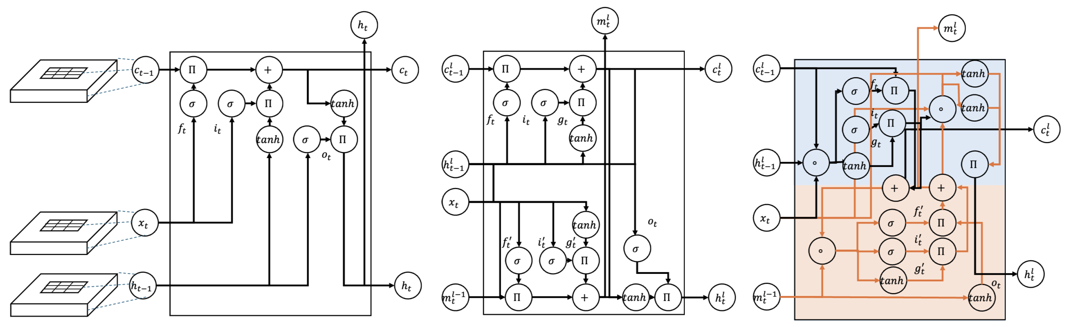
Figure 2.
Illustration of the bi-directional memory network showing the detailed processing within a single cascaded cell. This figure highlights the processing steps of convolutional operations, layer normalization, and memory state updates that occur within each cell. It provides an in-depth look at the integration process that combines information from the forward and backward paths, forming part of the comprehensive 4-layer architecture illustrated in the multi-layer implementation over time sequences.
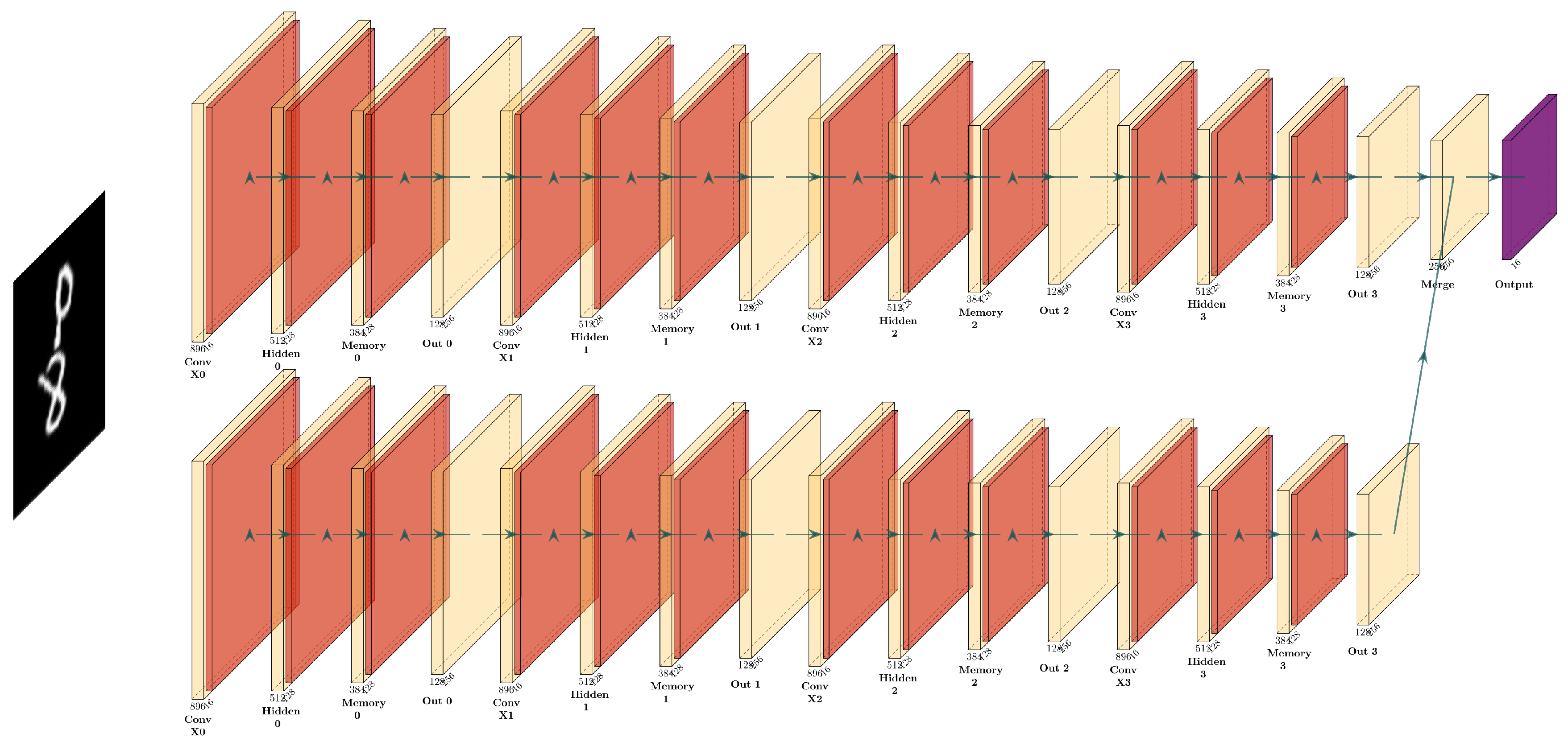
Figure 3.
Temporal evolution of the bi-directional memory network over two consecutive time steps (t=0 and t=1). Black arrows indicate information flow between cells, red arrows represent spatial memory state propagation within each time steps. Temporal connections between forward (top-to-bottom) and backward (bottom-to-top) passes are included for bi-directionality. Each time step processes input through 4-layer cascaded cells with spatial memory states flowing from higher to lower layers.
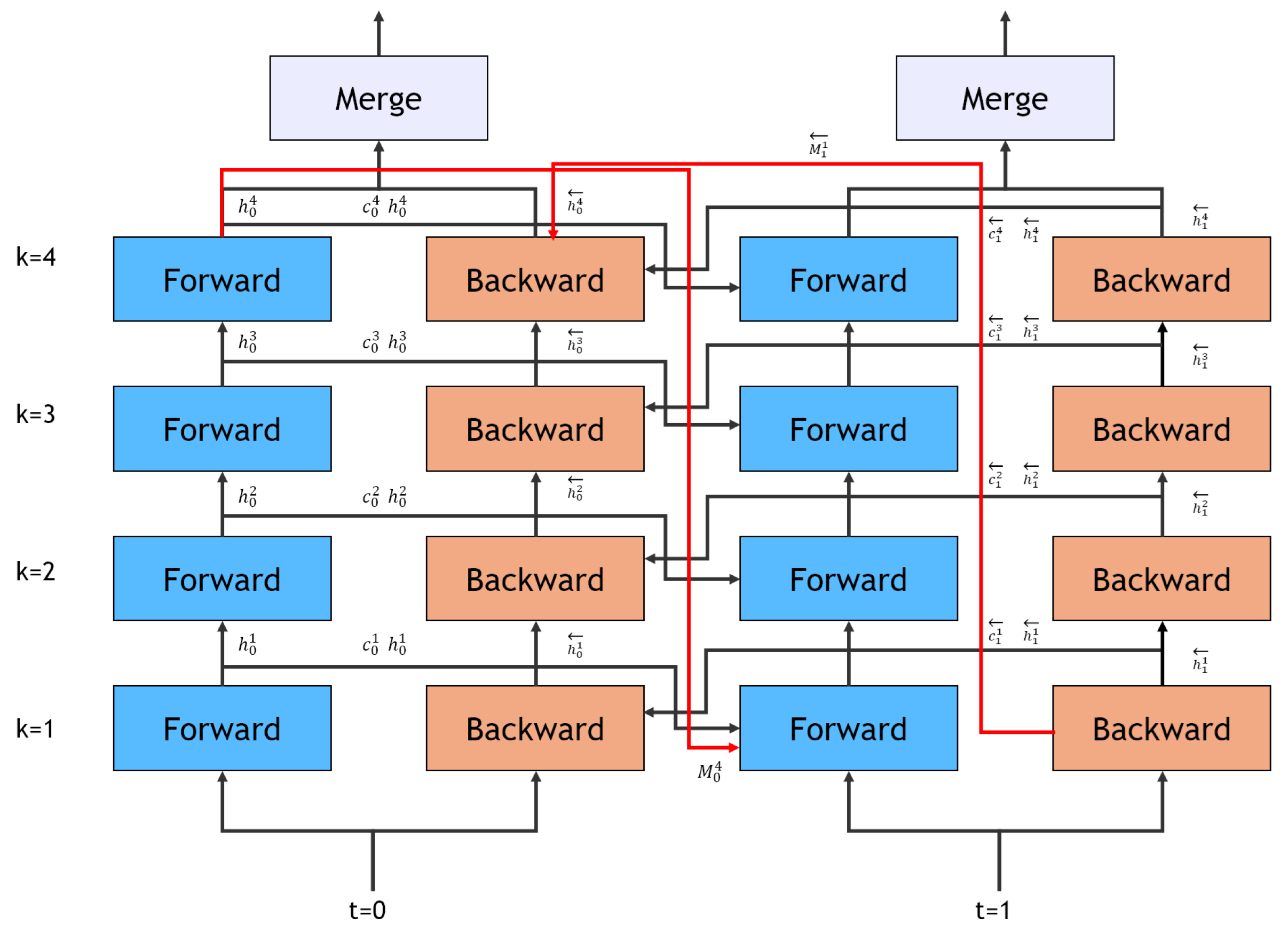
Figure 4.
Surface air temperature (climatological season cycle removed)
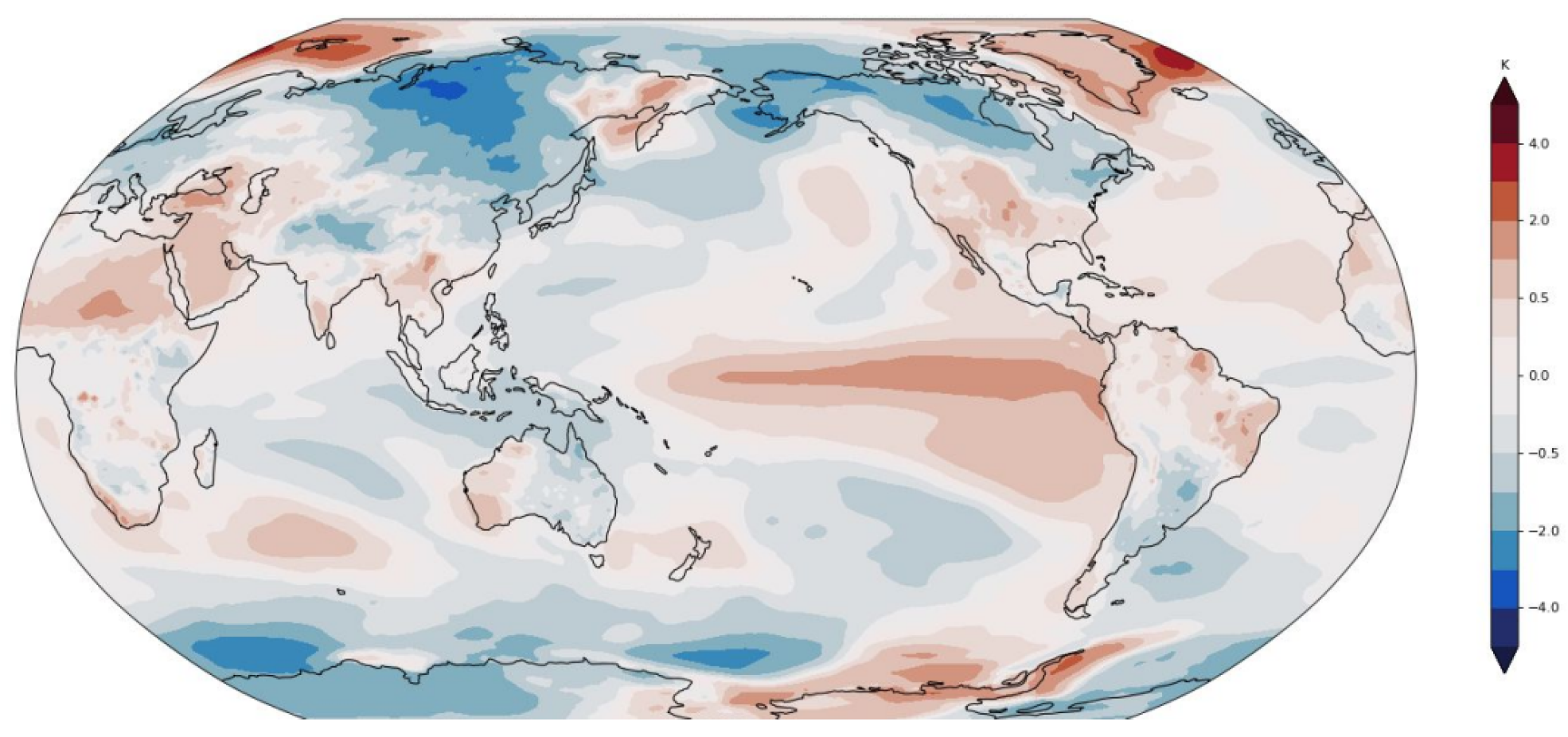
Figure 5.
Left: Moving MNIST prediction samples, Right: KTH prediction samples We predict 20 frames into the future by observing 10 frames.
Figure 5.
Left: Moving MNIST prediction samples, Right: KTH prediction samples We predict 20 frames into the future by observing 10 frames.
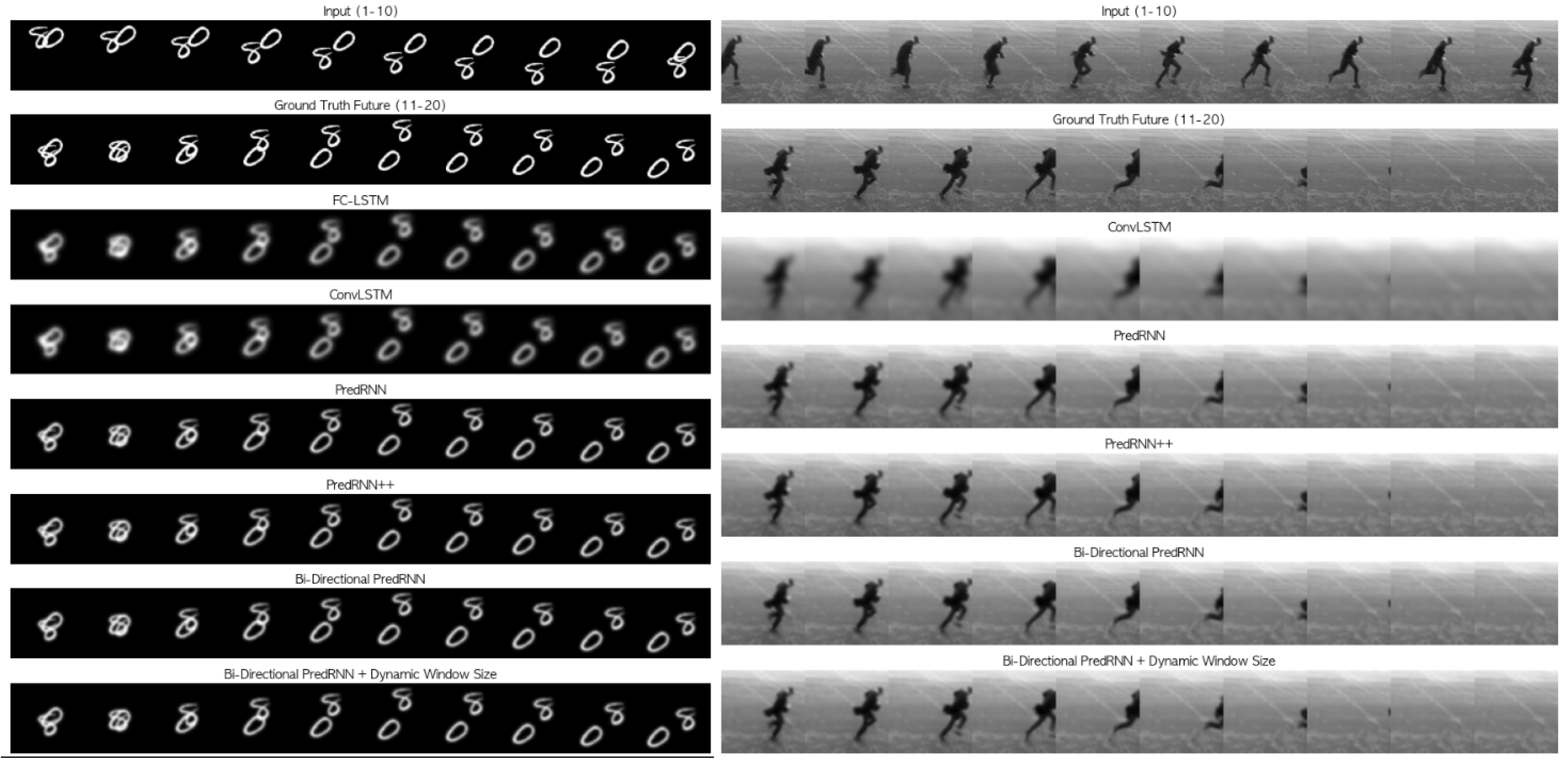

Table 1.
Comparison of Model Performance Across Different Datasets
| Model | MSE | PSNR | SSIM |
|---|---|---|---|
| Moving MNIST Dataset (10 time steps) | |||
| FC-LSTM | 118.30 | 27.40 | 0.69 |
| ConvLSTM | 103.30 | 27.99 | 0.71 |
| PredRNN | 56.80 | 30.59 | 0.87 |
| PredRNN++ | 50.70 | 31.08 | 0.89 |
| Bi-Directional PredRNN | 49.25 | 31.21 | 0.89 |
| Bi-Directional PredRNN + Dynamic Window Size | 47.60 | 31.34 | 0.90 |
| KTH Dataset (10 time steps) | |||
| ConvLSTM | 285.15 | 23.58 | 0.71 |
| PredRNN | 114.31 | 27.55 | 0.84 |
| PredRNN++ | 92.49 | 28.47 | 0.87 |
| Bi-Directional PredRNN | 98.79 | 29.16 | 0.75 |
| Bi-Directional PredRNN + Dynamic Window Size | 91.28 | 29.25 | 0.88 |
| ToSNA Dataset (30 frames) | |||
| ConvLSTM | 60.30 | 26.32 | 0.78 |
| PredRNN | 51.40 | 27.02 | 0.82 |
| Bi-Directional PredRNN | 49.60 | 27.18 | 0.83 |
| Bi-Directional PredRNN + Dynamic Window Size | 48.25 | 27.29 | 0.84 |
| Climate Dataset (30 frames) | |||
| ConvLSTM | 45.20 | 27.10 | 0.78 |
| PredRNN | 40.35 | 27.80 | 0.80 |
| Bi-Directional PredRNN | 38.50 | 28.20 | 0.81 |
| Bi-Directional PredRNN + Dynamic Window Size | 37.25 | 28.60 | 0.82 |
* Lower values are better for MSE, higher values are better for PSNR and SSIM.
Disclaimer/Publisher’s Note: The statements, opinions and data contained in all publications are solely those of the individual author(s) and contributor(s) and not of MDPI and/or the editor(s). MDPI and/or the editor(s) disclaim responsibility for any injury to people or property resulting from any ideas, methods, instructions or products referred to in the content. |
© 2024 by the authors. Licensee MDPI, Basel, Switzerland. This article is an open access article distributed under the terms and conditions of the Creative Commons Attribution (CC BY) license (http://creativecommons.org/licenses/by/4.0/).
Copyright: This open access article is published under a Creative Commons CC BY 4.0 license, which permit the free download, distribution, and reuse, provided that the author and preprint are cited in any reuse.


